
A trust‑region based sequential linear programming ...
33
This document is downloaded from DR‑NTU (https://dr.ntu.edu.sg) Nanyang Technological University, Singapore. A trust‑region based sequential linear programming approach for AC optimal power flow problems Sampath, Lahanda Purage Mohasha Isuru; Patil, Bhagyesh V.; Gooi, Hoay Beng; Maciejowski, Jan Marian; Ling, Keck Voon 2018 Sampath, L. P. M. I., Patil, B. V., Gooi, H. B., Maciejowski, J. M., & Ling, K. V. (2018). A trust‑region based sequential linear programming approach for AC optimal power flow problems. Electric Power Systems Research, 165, 134‑143. doi:10.1016/j.epsr.2018.09.002 https://hdl.handle.net/10356/137067 https://doi.org/10.1016/j.epsr.2018.09.002 © 2018 Elsevier B.V. All rights reserved. This paper was published in Electric Power Systems Research and is made available with permission of Elsevier B.V. Downloaded on 14 Mar 2022 12:29:54 SGT
Transcript of A trust‑region based sequential linear programming ...
This document is downloaded from DR‑NTU (https://dr.ntu.edu.sg)Nanyang Technological University, Singapore.
A trust‑region based sequential linearprogramming approach for AC optimal powerflow problems
Sampath, Lahanda Purage Mohasha Isuru; Patil, Bhagyesh V.; Gooi, Hoay Beng;Maciejowski, Jan Marian; Ling, Keck Voon
2018
Sampath, L. P. M. I., Patil, B. V., Gooi, H. B., Maciejowski, J. M., & Ling, K. V. (2018). Atrust‑region based sequential linear programming approach for AC optimal power flowproblems. Electric Power Systems Research, 165, 134‑143. doi:10.1016/j.epsr.2018.09.002
https://hdl.handle.net/10356/137067
https://doi.org/10.1016/j.epsr.2018.09.002
© 2018 Elsevier B.V. All rights reserved. This paper was published in Electric Power SystemsResearch and is made available with permission of Elsevier B.V.
Downloaded on 14 Mar 2022 12:29:54 SGT
A Trust-Region based Sequential Linear ProgrammingApproach for AC Optimal Power Flow Problems
L. P. M. I. Sampatha,∗, Bhagyesh V. Patilb,H. B. Gooic, J. M. Maciejowskid, K. V. Lingc
aInterdisciplinary Graduate School, Nanyang Technological University, SingaporebCambridge Centre for Advanced Research and Education in Singapore (CARES)
cSchool of Electrical and Electronic Engineering, Nanyang Technological University,Singapore
dDepartment of Engineering, University of Cambridge, United Kingdom and EnergyResearch Institute at NTU (ERI@N), Singapore.
Abstract
This study proposes a new trust-region based sequential linear programming
algorithm to solve the AC optimal power flow (OPF) problem. The OPF prob-
lem is solved by linearizing the cost function, power balance and engineering
constraints of the system, followed by a trust-region to control the validity of
the linear model. To alleviate the problems associated with the infeasibilities
of a linear approximation, a feasibility restoration phase is introduced. This
phase uses the original nonlinear constraints to quickly locate a feasible point
when the linear approximation is infeasible. The algorithm follows convergence
criteria to satisfy the first order optimality conditions for the original OPF prob-
lem. Studies on standard IEEE systems and large-scale Polish systems show an
acceptable quality of convergence to a set of best-known solutions and a sub-
stantial improvement in computational time, with linear scaling proportional to
the network size.
Keywords: Nonlinear programming, optimal power flow, sequential linear
programming, trust-region method.
∗Corresponding authorEmail address: [email protected] (L. P. M. I. Sampath)
Preprint submitted to Electric Power Systems Research September 5, 2018
1. Introduction1
The OPF problem optimizes the total operating cost to support efficient2
operation of power systems while satisfying system constraints for a nominal3
state [1]. In practice one needs to solve a security-constrained OPF (SC-OPF)4
problem which takes into account the possibility of a sudden failure of a single5
component (generator, transmission line, transformer, etc) in the system. This6
is known as the N−1 security criterion [1, 2]. The OPF problem without se-7
curity constraints has been extensively investigated in the literature (see, for8
instance [2], and references therein). This paper addresses the OPF problem9
for simplicity, but the benefits of our approach extend to the context of the10
SC-OPF problem as well. It is well-known that the OPF problem is nonlinear11
and nonconvex in nature, potentially having multiple equilibrium points. Hence12
searching for a global solution is in principle NP-hard (cf.[2, 3, 4, 5]). Electricity13
market clearing strategies are mainly based on nodal prices, which are the dual14
variables of power balance constraints of the OPF problem. This highlights15
the importance of the convexity and scalability features for any algorithm to16
use in OPF calculations [1, 6]. In addition to this, real-world OPF problems17
involve very large numbers of decision variables. This makes them challenging18
for a solution technique, both in terms of memory and computational time re-19
quirements. Consequently there is a great need for computationally efficient20
techniques which can handle the nonconvex AC network constraints.21
In the context of OPF, solution approaches, such as linear programming22
(LP) [6, 7, 8], quadratic programming (QP) [9], Lagrangian relaxation [10],23
and interior-point (IP) methods [11] have been extensively investigated in the24
literature. It is worth noting that, among all these approaches, IP methods25
have emerged as a promising direct solution approach for OPF problems. IP26
methods have proven to be a viable computational alternative for the solution of27
large-scale OPF problems [12]. The primal-dual logarithmic barrier IP method28
and its predictor-corrector variant are known to be efficient for OPF solution29
algorithms due to their superior computational efficiency [13]. We refer to [14]30
2

and references therein for a detailed survey of other solution approaches for the31
OPF problem.32
Many convexification approaches for power flow constraints have been pro-33
posed to make the AC-OPF problem computationally tractable. One of the34
widely used techniques in the last decade is semidefinite relaxation (SDR) which35
can find the global optimal solution of the OPF problem for radial networks36
under mild operating conditions [15, 16, 17, 18, 19]. However, in the case of37
meshed networks, SDR possesses a relaxation gap and necessitates the use of38
virtual phase shifters to recover bus voltage angles [20]. This can be an ex-39
pensive task in practice. Furthermore, semidefinite programs do not scale well40
for large-size power systems [21]. To circumvent the scalability issue associated41
with SDR, recently a second-order cone relaxation (SOCR) has been introduced.42
The SOCR enhances the computational performance, enabling the application43
of the technique for OPF problems in large-scale power networks [22, 23]. Based44
on SOCR, two different power flow formulations are considered in the literature,45
namely the bus injection model [21] and the branch flow model [22, 23]. Re-46
cently, the work in [24] introduced additional linear cuts in the branch flow47
framework to guarantee the exactness of SOCR for active distribution power48
networks. Similarly, an improved quadratic convex relaxation is proposed in49
[21] as an extension of SDR, in which voltage magnitudes are coupled with volt-50
age angles using additional polyhedral constraints. This improves the relaxation51
gap in comparison to SOCR without sacrificing the computational performance.52
However, a significant relaxation gap still persists in many power system cases53
[21]. Solution approaches based on the global optimization philosophy, such as54
convex envelopes [25] and decomposition methods [26] have also been reported55
in the literature.56
In the aforementioned approaches, LP methods can be an attractive can-57
didate for OPF problems due to their inherent scalable nature. Recent works58
[6, 27] have used successive linear programming (SLP)1 principles to demon-59
1The words ‘successive’ or ‘sequential’ are used interchangeably in the context of linear
3
strate this fact. Specifically, [6] has shown the scalability of LP tools against60
the well-known IP solver IPOPT [28] as well as the nonlinear optimization solver61
KNITRO [29]. In [5], rectangular form of complex quantities is used to formulate62
the power flow model, which disregards quasi-linear relationships of active power63
and bus voltage angles, and the reactive power and voltage magnitudes [5]. In64
addition, that formulation results in noncovex voltage limit constraints which65
need additional slack variables in order to be linearized.66
Note that SLP approaches can suffer from poor approximation of the original67
OPF problem due to lack of any globalization strategy. An SLP approach68
starting at an arbitrary point far from a solution to the original OPF may not69
converge to a feasible solution. In such circumstances, trust-region (TR) based70
methods have proven to be a viable alternative; see for instance TR-SE [30],71
TR-IP [31], [32] and TR-QP [33]. In TR methods, an approximation problem72
is solved within a small radius (called the trust-region). This enables a good73
approximation for the original OPF to be obtained at each solution step within74
the given trust-region.75
This paper proposes a synergistic approach based on a trust-region method76
and SLP for the OPF problem. Our approach is very much inspired by the77
recently proposed successive linearization scheme of [6] and the trust-region78
implementation [31]. However, our work differs in the following ways:79
• Unlike [6], we use the polar form of complex quantities. This assists in80
capturing the quasi-linear relationship between active power and bus volt-81
age angles, and the reactive power and voltage magnitudes for the original82
OPF problem.83
• In addition compared to [6], we propose a trust-region radius constraint84
to improve the validity of the linear approximations in subsequent SLP85
steps.86
programming approximation schemes. This work prefers to use the phrase ‘sequential linear
programming’.
4
• Further, compared to [31], instead of a penalty reformulation, we pro-87
pose a simple feasibility restoration phase based on the original nonlinear88
constraints, in order to avoid infeasibilities of intermediate linerizations.89
In brief, this work uses first-order Talyor series to construct a local linear model90
for the original OPF problem. A trust-region constraint is designed to ensure91
the validity of the constructed linear model, that is, to ensure that the original92
nonlinear constraints are satisfied. This is then integrated in an iterative pro-93
cedure to optimize bus voltage magnitudes and angles, and active and reactive94
power generation. This trust-region sequential linear program (TR-SLP) termi-95
nates in a finite number of iterations, returning an OPF solution satisfying the96
convergence criteria (see Section 3.4). The performance of TR-SLP is tested on97
various benchmark IEEE and Polish systems against the SLP approach in [6],98
NLP solvers IPOPT [28] and KNITRO [29]. The results of TR-SLP demon-99
strate an acceptable quality of convergence to the best-known solution for the100
considered benchmark systems.101
The paper presents the OPF problem formulation in Section 2, followed by102
the algorithm of TR-SLP in Section 3. Section 4 presents the numerical results103
on various IEEE networks. Finally, the paper is concluded in Section 5.104
2. Mathematical Formulation105
In this section, we first present the network model for a general power sys-106
tem and formulate the AC-OPF problem. Then, a linear programming (LP)107
approximation of the AC-OPF problem is derived using first-order Taylor se-108
ries. This linear approximation is later embedded in an iterative procedure to109
form the TR-SLP algorithm (see Section 3).110
2.1. Network Model111
We define N and L as the set of buses and the set of transmission lines of the112
power system respectively, where |N | = N and |L| = L. Further, let G (|G| = G)113
be the set of generators which are connected to a subset of N . To formulate114
5
the OPF problem, we use the polar form of the complex bus voltage v ∈ CN115
and its ith element vi = Viejδi , where Vi is the voltage magnitude and δi is the116
phase angle of the voltage phasor vi at bus i ∈ N . Complex power generation117
is denoted by sG ∈ CG such that sGg = PGg + jQG
g for generator g ∈ G, where118
PGg and QG
g are the active and reactive power generation respectively. These119
two vectors (v and sG) are the decision variables of the OPF problem. The120
parameters involved in the formulation are defined below.121
The standard π−model is applied for modeling transmission lines. For the122
transmission line l ∈ L, let Y ∈ CL be the branch admittance vector, having123
components Yl = gl(i,j) + jbl(i,j), where gl(i,j) and bl(i,j) are the series conduc-124
tance and susceptance respectively. Similarly, bshl(i,j) ∈ R is the line charging125
susceptance for tranmission line l. Complex power demand is characterized by126
sD ∈ CN such that sDi = PDi + jQD
i , where PDi and QD
i are the active and127
reactive power demand respectively at bus i.128
2.2. AC-OPF Problem Formulation129
The objective function of the OPF problem is generally formulated as the130
generation cost minimization. The constraints are formulated to satisfy the131
power balance at each bus, the generation capacity margins, and network con-132
straints, namely power flow limits and voltage bounds.133
The quadratic cost function for generator g in the system is represented134
below.135
Cg = c2,g(PGg
)2+ c1,gP
Gg + c0,g , ∀g ∈ G (1)
where c2,g, c1,g and c0,g denote the coefficients of quadratic, linear, and con-
stant terms of the cost function, respectively. Then the complete OPF can be
formulated as a NLP problem to optimize the total operating cost of the system:
minδi, Vi,
PGg , Q
Gg
∑g∈G
Cg (2a)
s.t.∑g∈G(i)
PGg − V 2
i
∑j∈N (i)
gl(i,j)
6
+ Vi∑
j∈N (i)
Vj[gl(i,j)cos(δi,j)− bl(i,j)sin(δi,j)
]= PD
i , ∀i ∈ N (2b)
∑g∈G(i)
QGg − V 2
i
∑j∈N (i)
(bl(i,j) + bshl(i,j)/2)
+ Vi∑
j∈N (i)
Vj[bl(i,j)cos(δi,j) + gl(i,j)sin(δi,j)
]= QD
i , ∀i ∈ N (2c)
I2l(i,j) ≤ (Imaxl )2, i, j ∈ N , ∀l ∈ L (2d)
I2l(j,i) ≤ (Imaxl )2, i, j ∈ N , ∀l ∈ L (2e)
I2l(i,j) = IAl(i,j)V2i + IBl(i,j)V
2j
− 2ViVj
[ICl(i,j)cos(δi,j)− IDl(i,j)sin(δi,j)
](2f)
Vi ∈[V mini , V max
i
], ∀i ∈ N (2g)
PGg ∈
[PG,ming , PG,max
g
], ∀g ∈ G (2h)
QGg ∈
[QG,ming , QG,max
g
], ∀g ∈ G (2i)
where δi,j = δi − δj ; constraints (2b) and (2c) represent the active and reactive
power balance at each bus; G(i) and N (i) are the set of generators connected at
bus i, and the set of buses connected to bus i by transmission lines, respectively;
and constraints (2d) and (2e) constrain the maximum current flow through each
transmission line. Here, (2f) models the apparent current flow from bus i to bus j
through transmission line l, where
IAl(i,j) = g2l(i,j) +(bl(i,j) + bshl(i,j)/2
)2,
IBl(i,j) = g2l(i,j) + b2l(i,j),
ICl(i,j) = g2l(i,j) + bl(i,j)
(bl(i,j) + bshl(i,j)/2
)and
IDl(i,j) = bl(i,j)bshl(i,j)/2 ;
The physical laws of power flow have been considered in modeling these con-136
straints. Constraint (2g) bounds the engineering limits of the voltage at each137
bus; and (2h) and (2i) bound the active and reactive power generation capabili-138
ties of each generator respectively; and (·)min and (·)max indicate the lower and139
upper bound of the decision variables, respectively. The optimization problem140
7

consists of 2(N + G) number of variables to optimize subject to the variable141
bounds and 2(N + L) number of constraints.142
2.3. LP Formulation143
The nonlinearity in the aforementioned OPF problem comes from equations
(1), (2b), (2c) and (2f). In our proposed iterative procedure (TR-SLP), the
nonlinear terms in these equations are linearized by applying first-order Tay-
lor series approximations evaluated at the solution of the previous iteration.
Assume the decision variable vector pertaining to the NLP problem (2) as
x : =[δ1, . . . , δN , V1, . . . , VN , P
G1 , . . . , P
GG , Q
G1 , . . . , Q
GG
]T ∈ R2(N+G).
where (·)T is the transpose operator. Then, the partial derivatives of (1), (2b),144
(2c) and (2f) are used to compute the Jacobian matrices as follows.145
JC,k−1 =
[0T2N ,
∂C1
∂PG1
, . . . ,∂CG∂PG
G
, 0TG
]∣∣∣∣xk−1
(3a)
PNi = V 2
i
∑j∈N (i)
gl(i,j)
− Vi∑
j∈N (i)
Vj[gl(i,j)cos(δi,j)− bl(i,j)sin(δi,j)
], ∀i ∈ N (3b)
JP,k−1i =
[∂PN
i
∂δ1, . . . ,
∂PNi
∂δN,∂PN
i
∂V1, . . . ,
∂PNi
∂VN, −eTG,i, 0T
G
]∣∣∣∣xk−1
, ∀i ∈ N (3c)
QNi = V 2
i
∑j∈N (i)
(bl(i,j) + bshl(i,j)/2)
− Vi∑
j∈N (i)
Vj[bl(i,j)cos(δi,j) + gl(i,j)sin(δi,j)
], ∀i ∈ N (3d)
JQ,k−1i =
[∂QN
i
∂δ1, . . . ,
∂QNi
∂δN,∂QN
i
∂V1, . . . ,
∂QNi
∂VN, 0T
G, −eTG,i]∣∣∣∣xk−1
, ∀i ∈ N (3e)
J I,k−1l(i,j) =
[∂I2l(i,j)
∂δ1, . . . ,
∂I2l(i,j)
∂δN,∂I2l(i,j)
∂V1, . . . ,
∂I2l(i,j)
∂VN, 0T
2G
]∣∣∣∣∣xk−1
,
i, j ∈ N , ∀l ∈ L (3f)
where 0(·) = {0}(·) and eG,i ∈ {0, 1}G, in which the gth element is 1 if gen-146
erator g ∈ G(i), or is 0 otherwise. PNi and QN
i denote the sum of active and147
8
reactive power extractions from bus i respectively; (·)k−1 denote the value of the148
decision variable/vector (·) at the (k − 1)th
iteration. Equations (3a), (3c), (3e)149
and (3f) represent the Jacobian matrices of (1), (2b), (2c) and (2f) respectively,150
which are originally nonlinear. At the kth iteration of TR-SLP, those Jacobian151
matrices in (3) are updated based on the solution of the previous (k − 1)th it-152
eration. Finally, the LP approximation of the OPF problem (2) to be solved at153
the kth iteration, obtained based on the solution of the (k − 1)th iteration, can154
be deduced as follows.155
LP(xk−1
)
minx
JC,k−1(x− xk−1) +∑g∈G
Cg|xk−1
s.t. JP,k−1i (x− xk−1) + PN
i
∣∣xk−1 −
∑g∈G(i)
PG,k−1g = −PD
i , ∀i ∈ N
JQ,k−1i
(x− xk−1
)+ QN
i
∣∣xk−1 −
∑g∈G(i)
QG,k−1g = −QD
i ,∀i ∈ N
J I,k−1l(i,j) (x− xk−1) + I2l(i,j)
∣∣∣xk−1
≤ (Imaxl )2, i, j ∈ N , ∀l ∈ L
J I,k−1l(j,i) (x− xk−1) + I2l(j,i)
∣∣∣xk−1
≤ (Imaxl )2, i, j ∈ N , ∀l ∈ L
(2g)− (2i)
(4)
It should be noted that (4) is tightly-coupled to the original OPF problem (2)156
at the evaluated point xk−1.157
3. Trust-Region based Sequential Linear Programming Algorithm158
This section first introduces components such as trust-region LP formulation,159
feasibility restoration phase and step acceptance/rejection criterion. Then the160
pseudo-code of the main algorithm TR-SLP comprising all these components161
is presented. For ease of explanation, the AC-OPF problem (2) is represented162
9
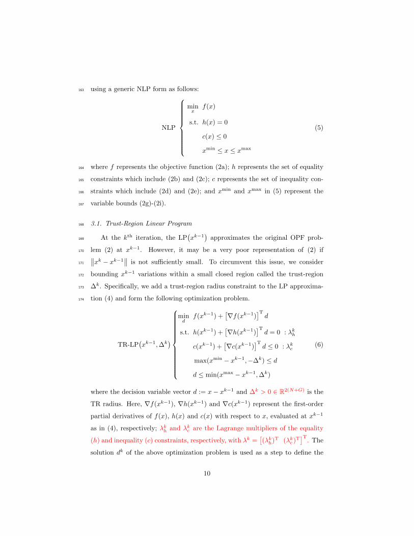
using a generic NLP form as follows:163
NLP
minx
f(x)
s.t. h(x) = 0
c(x) ≤ 0
xmin ≤ x ≤ xmax
(5)
where f represents the objective function (2a); h represents the set of equality164
constraints which include (2b) and (2c); c represents the set of inequality con-165
straints which include (2d) and (2e); and xmin and xmax in (5) represent the166
variable bounds (2g)-(2i).167
3.1. Trust-Region Linear Program168
At the kth iteration, the LP(xk−1
)approximates the original OPF prob-169
lem (2) at xk−1. However, it may be a very poor representation of (2) if170 ∥∥xk − xk−1∥∥ is not sufficiently small. To circumvent this issue, we consider171
bounding xk−1 variations within a small closed region called the trust-region172
∆k. Specifically, we add a trust-region radius constraint to the LP approxima-173
tion (4) and form the following optimization problem.174
TR-LP(xk−1,∆k
)
mind
f(xk−1) +[∇f(xk−1)
]Td
s.t. h(xk−1) +[∇h(xk−1)
]Td = 0 : λkh
c(xk−1) +[∇c(xk−1)
]Td ≤ 0 : λkc
max(xmin − xk−1,−∆k) ≤ d
d ≤ min(xmax − xk−1,∆k)
(6)
where the decision variable vector d := x− xk−1 and ∆k > 0 ∈ R2(N+G) is the
TR radius. Here, ∇f(xk−1), ∇h(xk−1) and ∇c(xk−1) represent the first-order
partial derivatives of f(x), h(x) and c(x) with respect to x, evaluated at xk−1
as in (4), respectively; λkh and λkc are the Lagrange multipliers of the equality
(h) and inequality (c) constraints, respectively, with λk =[(λkh)T (λkc )T
]T. The
solution dk of the above optimization problem is used as a step to define the
10

new solution approximation, i.e. xk = xk−1 + dk (see Section 3.3). The Karush-
Kuhn-Tucker (KKT) conditions for (6) are:
h(xk−1) +[∇h(xk−1)
]Tdk = 0 (7a)
c(xk−1) +[∇c(xk−1)
]Tdk ≤ 0 (7b)
∇f(xk−1) +∇c(xk−1)λkc +∇h(xk−1)λkh = 0 (7c)(c(xk−1) +
[∇c(xk−1)
]Tdk)λkc = 0 (7d)
λkc ≥ 0 (7e)
Equations (7) will be satisfied at every successful TR-LP computation.175
It should be noted that a smaller TR radius may cause constraint infeasibil-176
ities or may reduce the speed of convergence. Similarly, a larger TR radius will177
weaken the validity of linear models that represent nonlinear constraints in (2).178
Therefore ∆k is modified at each step of the algorithm (step 6 of Algorithm 1),179
the modification depending on the improvement in optimality.180
3.2. Feasibility Restoration181
In practice, TR-LP(xk−1,∆k
)can be infeasible due to the following two182
reasons: i) The constraint gradients[∇h(xk−1)
]Tcan become degenerate at183
the point xk−1, leading to infeasible linearized constraints. Then the system184 [∇h(xk−1)
]Td = −h(xk−1) simply has no solution. ii) If the trust-region is185
too small, the TR-LP may be infeasible. In such circumstances, the linear186
constraint, h(xk−1) +[∇h(xk−1)
]Td = 0, cannot be satisfied within the trust-187
region radius ∆k of xk−1.188
Feasibility restoration (NLP-FR) searches for a feasible point by solving the189
following problem, so that the next TR-LP subproblem to be solved will be190
11

feasible.191
NLP-FR
minx, sc,
s+h , s−h
sc + s+h + s−h
s.t. c(x)− sc ≤ 0
h(x)− s+h + s−h = 0
xmin ≤ x ≤ xmax
sc, s+h , s
−h ≥ 0
(8)
where sc, s+h , s
−h are slack variables used to relax the inequality and equality192
constraints respectively.193
If the NLP-FR cannot find a solution with zero objective value, then the194
OPF problem (2) is declared as infeasible. Otherwise, we have found a feasible195
point xk, which is used to compute the step-size dk := xk − xk−1.196
3.3. Step Acceptance/Rejection Criterion197
To accept or reject the new step-size dk and update the trust-region radius198
∆k for the next TR-SLP iteration, we compute the ratio ρk between predicted199
and actual reduction in the cost function (2a).200
Let dk be a solution of TR-LP(xk−1,∆k
). Then the predicted reduction in201
the objective is202
∆φkpre =[∇f(xk−1)
]Tdk. (9)
In order to take into account any constraint violations, as well as the actual203
value of the objective of the NLP (5), the following merit function is defined:204
φ(xk) = f(xk) + (νkh)T|h(xk)|+ (νkc )T max{c(xk), 0}, (10)
where νkh ∈ Rnh+ and νkc ∈ Rnc
+ are penalty factors for equality and inequality
constraints respectively. These are derived in each iteration k based on (11a)
and (11b) using dual variables λkh and λkc as follows.
νkh = max{νk−1h , λkh} (11a)
νkc = max{νk−1c , λkc} (11b)
12
ν0h,m =‖ ∇f(x0) ‖2‖ ∇hm(x0) ‖2
, ∀m ∈ {1, . . . , nh} (11c)
ν0c,m =‖ ∇f(x0) ‖2‖ ∇cm(x0) ‖2
, ∀m ∈ {1, . . . , nc} (11d)
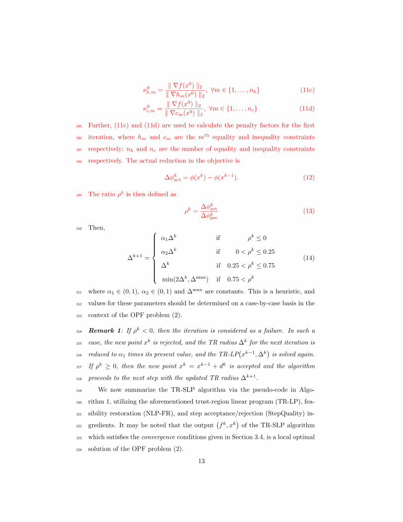
Further, (11c) and (11d) are used to calculate the penalty factors for the first205
iteration, where hm and cm are the mth equality and inequality constraints206
respectively; nh and nc are the number of equality and inequality constraints207
respectively. The actual reduction in the objective is208
∆φkact = φ(xk)− φ(xk−1). (12)
The ratio ρk is then defined as209
ρk =∆φkact∆φkpre
(13)
Then,210
∆k+1 =
α1∆k if ρk ≤ 0
α2∆k if 0 < ρk ≤ 0.25
∆k if 0.25 < ρk ≤ 0.75
min(2∆k,∆max) if 0.75 < ρk
(14)
where α1 ∈ (0, 1), α2 ∈ (0, 1) and ∆max are constants. This is a heuristic, and211
values for these parameters should be determined on a case-by-case basis in the212
context of the OPF problem (2).213
Remark 1: If ρk < 0, then the iteration is considered as a failure. In such a214
case, the new point xk is rejected, and the TR radius ∆k for the next iteration is215
reduced to α1 times its present value, and the TR-LP(xk−1,∆k
)is solved again.216
If ρk ≥ 0, then the new point xk = xk−1 + dk is accepted and the algorithm217
proceeds to the next step with the updated TR radius ∆k+1.218
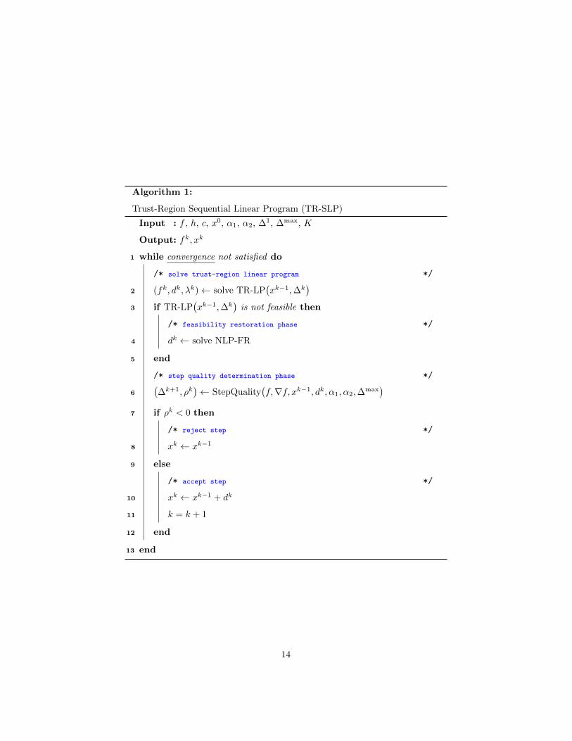
We now summarize the TR-SLP algorithm via the pseudo-code in Algo-219
rithm 1, utilizing the aforementioned trust-region linear program (TR-LP), fea-220
sibility restoration (NLP-FR), and step acceptance/rejection (StepQuality) in-221
gredients. It may be noted that the output(fk, xk
)of the TR-SLP algorithm222
which satisfies the convergence conditions given in Section 3.4, is a local optimal223
solution of the OPF problem (2).224
13
Algorithm 1:
Trust-Region Sequential Linear Program (TR-SLP)
Input : f , h, c, x0, α1, α2, ∆1, ∆max, K
Output: fk, xk
1 while convergence not satisfied do
/* solve trust-region linear program */
2 (fk, dk, λk)← solve TR-LP(xk−1,∆k
)3 if TR-LP
(xk−1,∆k
)is not feasible then
/* feasibility restoration phase */
4 dk ← solve NLP-FR
5 end
/* step quality determination phase */
6(∆k+1, ρk
)← StepQuality
(f,∇f, xk−1, dk, α1, α2,∆
max)
7 if ρk < 0 then
/* reject step */
8 xk ← xk−1
9 else
/* accept step */
10 xk ← xk−1 + dk
11 k = k + 1
12 end
13 end
14

3.4. Discussion on Convergence225
We first give the necessary Karush-Kuhn-Tucker (KKT) conditions adopted226
from [34] for TR-SLP described in Algorithm 1. The TR-SLP stops when the227
following conditions are satisfied.228
(a) ‖ dk ‖∞ ≤ εd229
(b) ‖ h(xk) ‖∞≤ ε, max{c(xk)} ≤ ε230
(c) max{‖ ∇f(xk)+∇c(xk)λkc+∇h(xk)λkh ‖∞, ‖ c(xk)λkc ‖∞} < ελ(1+ ‖ λk ‖2
)231
(d) λkc ≥ 0232
where εd, ε, and ελ are tolerances chosen for the step change, constraint satis-233
faction and KKT condition satisfaction respectively. Condition (a) implies that234
the step-size has reached the user-specified accuracy εd. Condition (b) implies235
that within the trust-region radius, the original nonlinear constraints h and c236
in the NLP (5) are satisfied to a user-specified accuracy of ε. Conditions (c)237
and (d) provide a measure of the closeness of the computed solution to a point238
satisfying the first-order optimality conditions for the NLP problem (5).239
To establish the convergence of TR-SLP (Algorithm 1) consider the follow-240
ing. TR-SLP solves a trust-region linear approximation (i.e. TR-LP (6)) of the241
original NLP (5) at each iteration k. If TR-LP is feasible, it will compute dk242
(step 2). Subsequently, based on the previous iterates xk−1 and dk, the actual-243
to-predicted cost ratio ρk and the new trust-region radius ∆k+1 are determined244
(step 6). Then, based on ρk, as the TR-SLP progresses, ∆k+1 shrinks, ensuring245
the tightness of the linear approximation TR-LP (cf. Figure 4). This leads the246
successive iterates xk to converge to a local solution of NLP (5), satisfying the247
conditions (a)–(d).248
4. Numerical Experiments and Discussion249
In this section, we report numerical results with the proposed TR-SLP al-250
gorithm for OPF problem (2). The TR-SLP is analyzed on a benchmark test251
15

suite consisting of IEEE (14, 30, 57, 118 and 300) systems, and Polish 2383wp,252
2746wop and 3012wp systems (the number refers to the number of buses in the253
respective test case) available in [35]. We note that [6] is a recent computational254
study on the AC-OPF problem for the aforementioned systems. It reports the255
OPF (2) results using general purpose optimization solvers like IPOPT [28] and256
KNITRO [29], and a penalty reformulations based successive linear program-257
ming (SLP) method. In [6], two types of OPF problems are solved for each258
system, viz. without line flow limits (baseline case), and with line flow lim-259
its (thermally constrained case). We obtain the line flow limits data for this260
work from [6, Table II]. Further, [6, Tables IV, V] report the results obtained261
using their proposed SLP, NLP solvers IPOPT and KNITRO for the various262
benchmark IEEE and Polish systems. These results have been obtained with263
constraint satisfaction up to 0.001 tolerance. We shall use these results in our264
study to compare the performance of our TR-SLP in terms of optimality and265
computational time.266
Convergence and optimality of the solution of SLP algorithms depend on the267
selected initial point (cf. [6]). In this study, we consider two different initializa-268
tion strategies for TR-SLP, viz, flat start and DC warm start, to demonstrate269
the variation of performance with respect to the starting point. In the flat270
start, we assume unit voltage phasors and half-max outputs for all generation.271
The DC warm start is constructed with the solution obtained from the DC-272
OPF problem combined with unit voltage magnitudes and half-max reactive273
power generation. We conduct three case studies to showcase the performance274
of the TR-SLP. Firstly, the computational time of the TR-SLP with the afore-275
mentioned test cases is compared against that of KNITRO, IPOPT and SLP.276
Secondly, we study the optimality of the solution obtained using the TR-SLP277
for the same test cases against the KNITRO solver run in a multi-start mode278
(henceforth referred as KNITRO-MS). We note that KNITRO run in a multi-279
start mode results in improved local optimal solutions [29]. Finally, we tighten280
the tolerances (i.e. εd, ε, ελ in TR-SLP) and study the relative improvement281
in the optimality of the solution obtained using the TR-SLP for the same test282
16
cases, and note the trade-off against computation time.283
The TR-SLP algorithm is implemented in MATLAB and the optimization284
problems are formulated based on the MATPOWER library [35]. The LP sub-285
problems are solved using CPLEX 12.6 [36] and feasibility restoration subprob-286
lems using the MATLAB fmincon solver based on the interior-point method.287
All experiments are carried out on a desktop PC with an IntelrCore i7-5500U288
4 core CPU processor running at 2.40GHz with 8GB RAM. Based on our ex-289
perience with the numerical experiments reported in this work, the parameters290
of TR-SLP are chosen as follows: α1 = 0.1, α2 = 0.25, ∆(0) = 0.4, ∆max = 2,291
K = 30, εd = 0.1, ε = ελ = 0.01. Note that, in all our numerical studies, the292
original nonlinear constraints (2b)−(2e) are satisfied up to the same accuracy293
employed by [6] (i.e. 0.001 or lesser).294
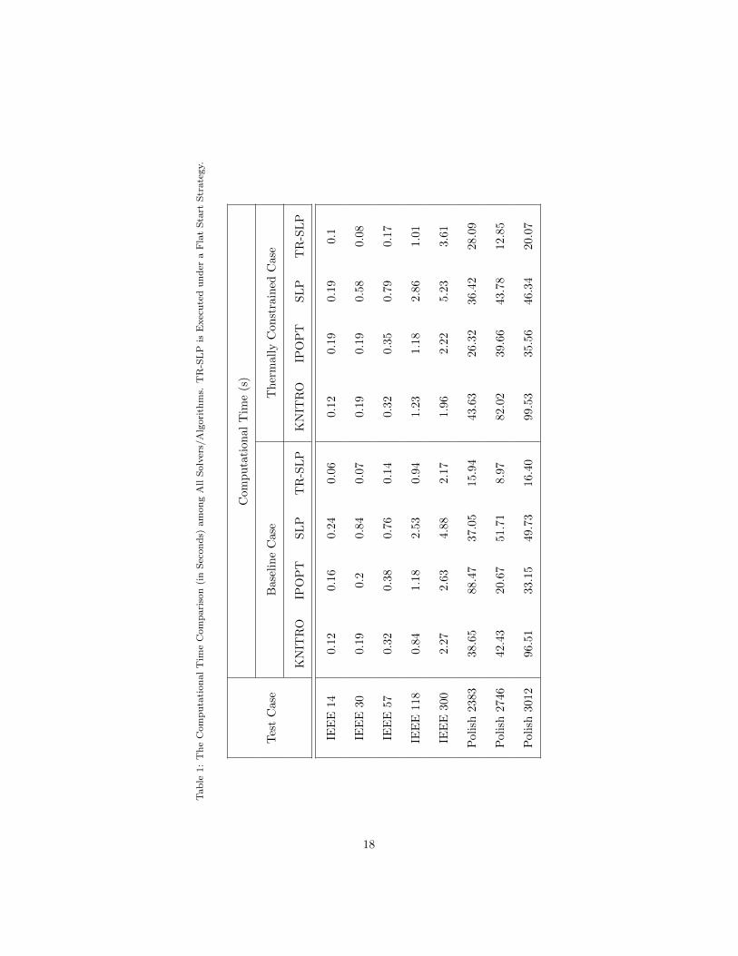
4.1. Case Study 1: Computational Time Comparison295
In this study, TR-SLP is executed with a flat start strategy for OPF problem296
(2) and is compared in Table 1 with different solution approaches for several297
test cases. It should be noted that in [6], four different initialization strategies,298
viz. flat start, DC warm start, AC warm start and uniform cold start are used299
and the best solver time recorded for each test case is reported (see Table 1;300
KNITRO, IPOPT, and SLP).301
It can be observed that for all IEEE systems, the CPU times of KNITRO302
and IPOPT are almost the same. Comparatively in Polish systems, KNITRO303
is noted to be slower. SLP is found to be the slowest for all IEEE systems.304
However, its performance is observed to improve for Polish systems with re-305
spect to KNITRO and IPOPT. We observed TR-SLP to be fastest among all306
solution approaches in many test cases (except IEEE 300 and Polish 2383 ther-307
mally constrained cases, where KNITRO and IPOPT are slightly faster). The308
TR-SLP reports comparatively the best CPU time for the largest Polish 3012309
system, approximately 6, 2 and 3 times faster than KNITRO, IPOPT, and SLP,310
respectively, for the baseline case and approximately 5, 1.5 and 2 times faster311
than KNITRO, IPOPT, and SLP, respectively, for the thermally constrained312
17
Tab
le1:
Th
eC
om
pu
tati
on
al
Tim
eC
om
pari
son
(in
Sec
on
ds)
am
on
gA
llS
olv
ers/
Alg
ori
thm
s.T
R-S
LP
isE
xec
ute
du
nd
era
Fla
tS
tart
Str
ate
gy.
Com
pu
tati
on
al
Tim
e(s
)
Tes
tC
ase
Bas
elin
eC
ase
Th
erm
all
yC
on
stra
ined
Case
KN
ITR
OIP
OP
TS
LP
TR
-SL
PK
NIT
RO
IPO
PT
SL
PT
R-S
LP
IEE
E14
0.12
0.1
60.2
40.0
60.1
20.
19
0.1
90.
1
IEE
E30
0.19
0.2
0.8
40.0
70.1
90.
19
0.5
80.
08
IEE
E57
0.32
0.3
80.7
60.1
40.3
20.
35
0.7
90.
17
IEE
E11
80.
841.1
82.5
30.9
41.2
31.
18
2.8
61.
01
IEE
E30
02.
272.6
34.8
82.1
71.9
62.
22
5.2
33.
61
Pol
ish
2383
38.6
588.4
737.0
515.
94
43.
63
26.
32
36.4
228.
09
Pol
ish
2746
42.4
320.6
751.7
18.
97
82.
02
39.
66
43.7
812.
85
Pol
ish
3012
96.5
133.1
549.7
316.
40
99.
53
35.
56
46.3
420.
07
18
case.
118 300 2383 2746 3012(a) Test Case (Baseline)
0
50
100
Tim
e (s
)
KNITROIPOPTSLPTR-SLP
118 300 2383 2746 3012(b) Test Case (Thermally Constrained)
0
50
100
Tim
e (s
)
KNITROIPOPTSLPTR-SLP
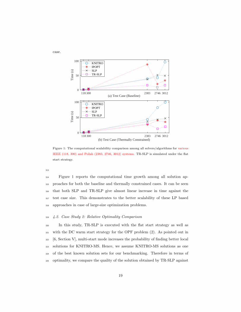
Figure 1: The computational scalability comparison among all solvers/algorithms for various
IEEE (118, 300) and Polish (2383, 2746, 3012) systems. TR-SLP is simulated under the flat
start strategy.
313
Figure 1 reports the computational time growth among all solution ap-314
proaches for both the baseline and thermally constrained cases. It can be seen315
that both SLP and TR-SLP give almost linear increase in time against the316
test case size. This demonstrates to the better scalability of these LP based317
approaches in case of large-size optimization problems.318
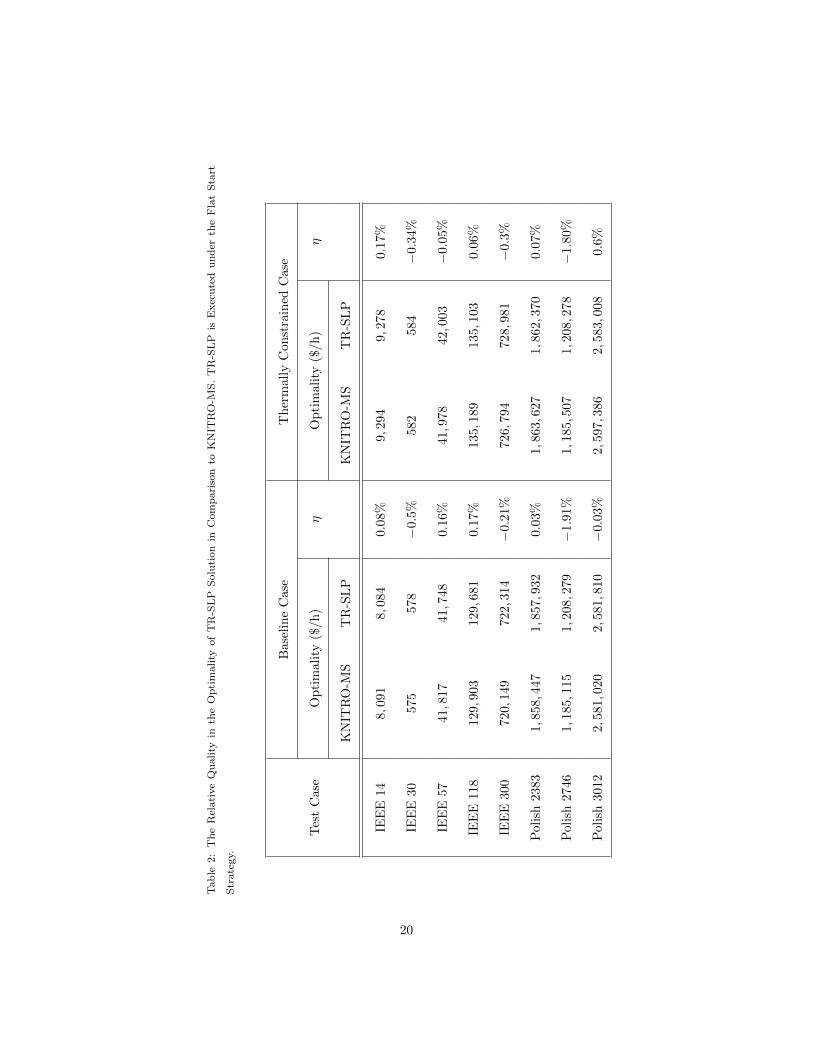
4.2. Case Study 2: Relative Optimality Comparison319
In this study, TR-SLP is executed with the flat start strategy as well as320
with the DC warm start strategy for the OPF problem (2). As pointed out in321
[6, Section V], multi-start mode increases the probability of finding better local322
solutions for KNITRO-MS. Hence, we assume KNITRO-MS solutions as one323
of the best known solution sets for our benchmarking. Therefore in terms of324
optimality, we compare the quality of the solution obtained by TR-SLP against325
19
Tab
le2:
Th
eR
elati
ve
Qu
ality
inth
eO
pti
mality
of
TR
-SL
PS
olu
tion
inC
om
pari
son
toK
NIT
RO
-MS
.T
R-S
LP
isE
xec
ute
du
nd
erth
eF
lat
Sta
rt
Str
ate
gy.
Bas
elin
eC
ase
Th
erm
all
yC
on
stra
ined
Case
Tes
tC
ase
Op
tim
alit
y($/h
)η
Op
tim
ali
ty($/h
)η
KN
ITR
O-M
ST
R-S
LP
KN
ITR
O-M
ST
R-S
LP
IEE
E14
8,09
18,0
84
0.08%
9,294
9,2
78
0.1
7%
IEE
E30
575
578
−0.
5%
582
584
−0.
34%
IEE
E57
41,8
1741,7
48
0.16%
41,9
78
42,0
03
−0.
05%
IEE
E11
812
9,9
0312
9,6
81
0.17%
135,1
89
135,1
03
0.0
6%
IEE
E30
072
0,1
4972
2,3
14
−0.
21%
726,7
94
728,9
81
−0.3
%
Pol
ish
2383
1,85
8,4
471,
857,9
32
0.03%
1,863,6
27
1,862,3
70
0.0
7%
Pol
ish
2746
1,18
5,1
151,
208,2
79
−1.
91%
1,185,5
07
1,208,2
78
−1.
80%
Pol
ish
3012
2,58
1,0
202,
581,8
10
−0.
03%
2,597,3
86
2,583,0
08
0.6%
20

Tab
le3:
Th
eR
elati
ve
Qu
ali
tyin
the
Op
tim
ality
of
TR
-SL
PS
olu
tion
inC
om
pari
son
toK
NIT
RO
-MS
.T
R-S
LP
isE
xec
ute
du
nd
erth
eD
CW
arm
Sta
rtS
trate
gy.
Bas
elin
eC
ase
Th
erm
all
yC
on
stra
ined
Case
Tes
tC
ase
Op
tim
alit
y($/h
)η
Op
tim
ali
ty($/h
)η
KN
ITR
O-M
ST
R-S
LP
KN
ITR
O-M
ST
R-S
LP
IEE
E14
8,09
18,0
88
0.03%
9,294
9,2
70
0.2
6%
IEE
E30
575
575
0%
582
583
−0.
51%
IEE
E57
41,8
1741,7
69
0.15%
41,9
78
41,9
61
0.0
4%
IEE
E11
812
9,9
0312
9,8
95
0%
135,1
89
135,0
17
0.1
3%
IEE
E30
072
0,1
4972
0,4
14
−0.
03%
726,7
94
726,1
92
0.0
8%
Pol
ish
2383
1,85
8,4
471,
857,9
29
0.03%
1,863,6
27
1,862,3
77
0.0
7%
Pol
ish
2746
1,18
5,1
151,
208,2
77
−1.
91%
1,185,5
07
1,208,2
81
−1.
80%
Pol
ish
3012
2,58
1,0
202,
581,8
10
−0.
03%
2,597,3
86
2,583,0
08
0.6%
21

the KNITRO-MS solution. For Table 2 and Table 3, we define the following326
performance metric:327
η =KNITRO-MS− TR-SLP
KNITRO-MS× 100% (15)
where η indicates the relative improvement (if η is positive) or deterioration (if328
η is negative) in optimality of the solution obtained by TR-SLP with respect to329
the best known KNITRO-MS solution.330
Table 2 reports the optimal solution obtained using KNITRO-MS and TR-331
SLP (with the flat start strategy) for the baseline and thermally constrained332
cases. In both cases, it can be observed that for half of the IEEE and Polish333
systems, TR-SLP results in slightly improved optimality with respect to the334
KNITRO-MS (ranging 0.03 % to 0.17 %). Performance of TR-SLP for the335
Polish 2746 system is observed to be slightly suboptimal for both the baseline336
and thermally constrained cases. However, KNITRO-MS is computationally337
slower than TR-SLP due to the multi-start feature, and represents a trade-off338
for using multi-start in practical OPF applications.339
Table 3 reports the optimal solution obtained using KNITRO-MS and TR-340
SLP with DC warm start strategy for the baseline and thermally constrained341
cases. The convergence and optimality of the solution of TR-SLP depends upon342
the initial point. As such we noted TR-SLP with the DC warm start strategy343
locates slightly different optimal values compared to those of TR-SLP with the344
flat start strategy. Hence, in order to compare the relative effectiveness between345
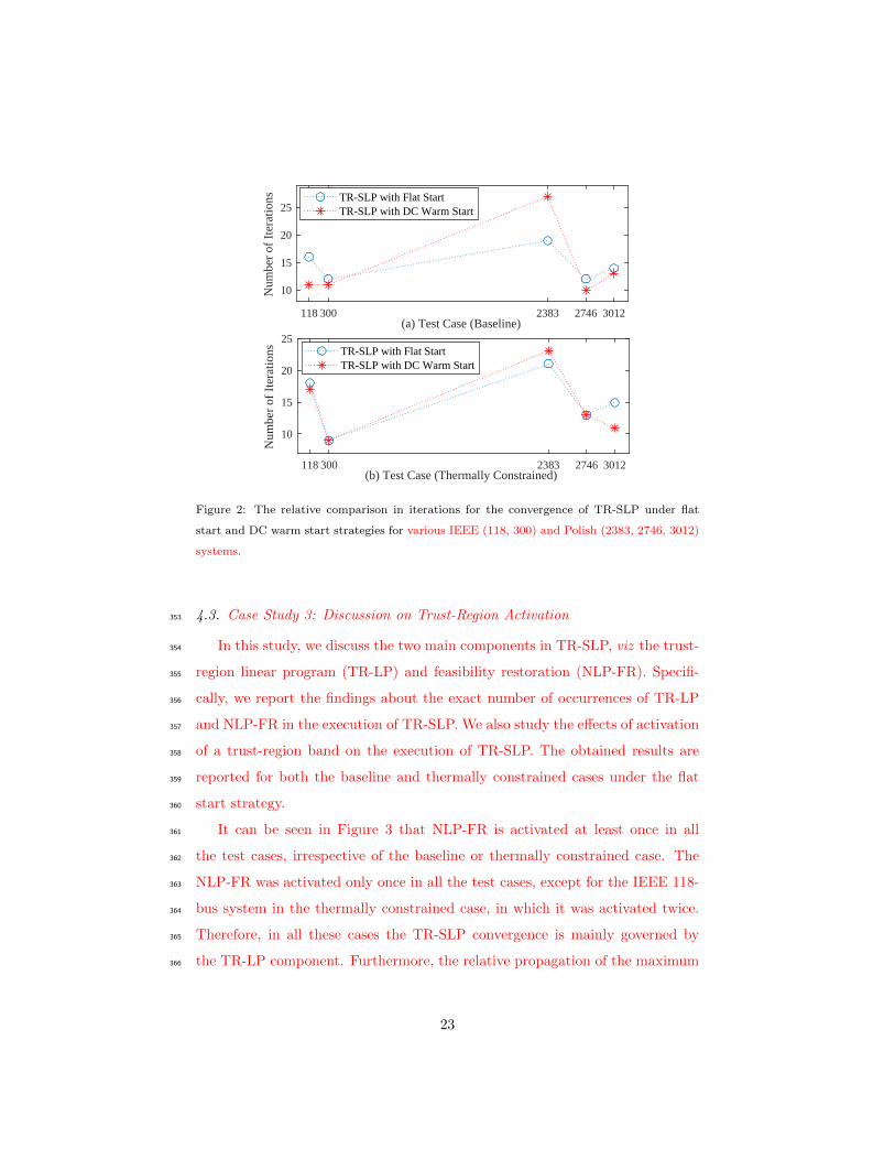
the flat start and DC warm start strategies, we analyze the number of iterations346
taken under each strategy to converge to the final solution. Figure 2 depicts347
the TR-SLP iterations of the IEEE (118, 300) and Polish (2383, 2746, 3012)348
systems for both the baseline and thermally constrained cases. We observe that349
the DC warm start strategy speeds up the convergence compared to the flat start350
strategy, except for the Polish 2383 system. However, both strategies converge351
within the maximum number of iterations set for TR-SLP, i.e. K = 30.352
22
118 300 2383 2746 3012(a) Test Case (Baseline)
10
15
20
25
Num
ber
of I
tera
tions TR-SLP with Flat Start
TR-SLP with DC Warm Start
118 300 2383 2746 3012(b) Test Case (Thermally Constrained)
10
15
20
25
Num
ber
of I
tera
tions TR-SLP with Flat Start
TR-SLP with DC Warm Start
Figure 2: The relative comparison in iterations for the convergence of TR-SLP under flat
start and DC warm start strategies for various IEEE (118, 300) and Polish (2383, 2746, 3012)
systems.
4.3. Case Study 3: Discussion on Trust-Region Activation353
In this study, we discuss the two main components in TR-SLP, viz the trust-354
region linear program (TR-LP) and feasibility restoration (NLP-FR). Specifi-355
cally, we report the findings about the exact number of occurrences of TR-LP356
and NLP-FR in the execution of TR-SLP. We also study the effects of activation357
of a trust-region band on the execution of TR-SLP. The obtained results are358
reported for both the baseline and thermally constrained cases under the flat359
start strategy.360
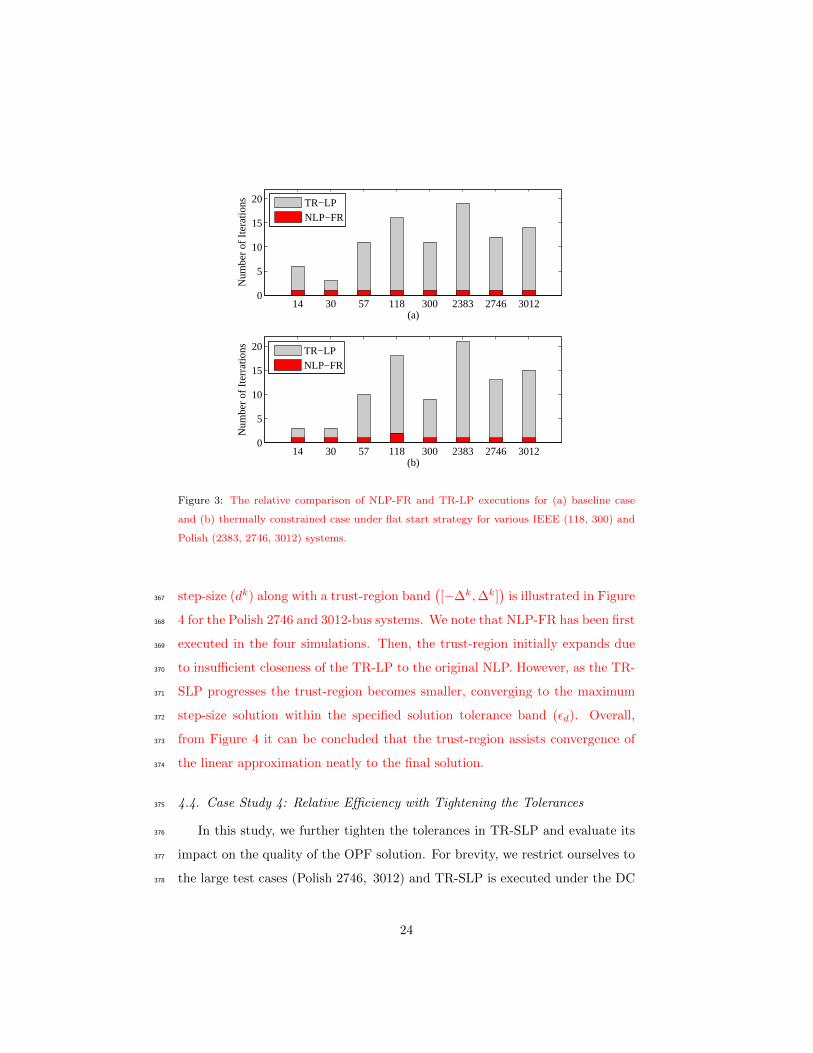
It can be seen in Figure 3 that NLP-FR is activated at least once in all361
the test cases, irrespective of the baseline or thermally constrained case. The362
NLP-FR was activated only once in all the test cases, except for the IEEE 118-363
bus system in the thermally constrained case, in which it was activated twice.364
Therefore, in all these cases the TR-SLP convergence is mainly governed by365
the TR-LP component. Furthermore, the relative propagation of the maximum366
23
14 30 57 118 300 2383 2746 30120
5
10
15
20
(a)
Num
ber
of It
erat
ions
14 30 57 118 300 2383 2746 30120
5
10
15
20
(b)
Num
ber
of It
erra
tions
TR−LPNLP−FR
TR−LPNLP−FR
Figure 3: The relative comparison of NLP-FR and TR-LP executions for (a) baseline case
and (b) thermally constrained case under flat start strategy for various IEEE (118, 300) and
Polish (2383, 2746, 3012) systems.
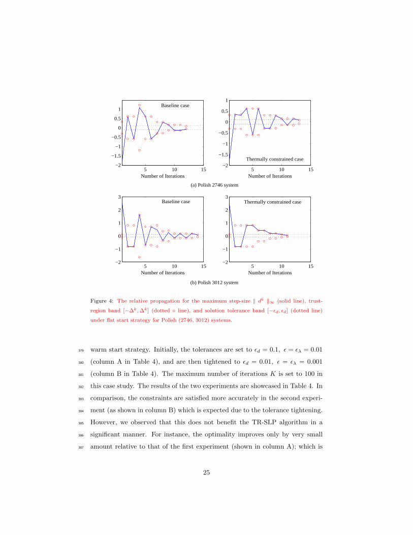
step-size (dk) along with a trust-region band([−∆k,∆k]
)is illustrated in Figure367
4 for the Polish 2746 and 3012-bus systems. We note that NLP-FR has been first368
executed in the four simulations. Then, the trust-region initially expands due369
to insufficient closeness of the TR-LP to the original NLP. However, as the TR-370
SLP progresses the trust-region becomes smaller, converging to the maximum371
step-size solution within the specified solution tolerance band (εd). Overall,372
from Figure 4 it can be concluded that the trust-region assists convergence of373
the linear approximation neatly to the final solution.374
4.4. Case Study 4: Relative Efficiency with Tightening the Tolerances375
In this study, we further tighten the tolerances in TR-SLP and evaluate its376
impact on the quality of the OPF solution. For brevity, we restrict ourselves to377
the large test cases (Polish 2746, 3012) and TR-SLP is executed under the DC378
24
5 10 15−2
−1.5
−1
−0.5
0
0.5
1
Number of Iterations5 10 15
−2
−1.5
−1
−0.5
0
0.5
1
Number of Iterations
5 10 15−2
−1
0
1
2
3
Number of Iterations5 10 15
−2
−1
0
1
2
3
Number of Iterations
Thermally constrained caseBaseline case
Baseline case
Thermally constrained case
(a) Polish 2746 system
(b) Polish 3012 system
Figure 4: The relative propagation for the maximum step-size ‖ dk ‖∞ (solid line), trust-
region band [−∆k,∆k] (dotted ◦ line), and solution tolerance band [−εd, εd] (dotted line)
under flat start strategy for Polish (2746, 3012) systems.
warm start strategy. Initially, the tolerances are set to εd = 0.1, ε = ελ = 0.01379
(column A in Table 4), and are then tightened to εd = 0.01, ε = ελ = 0.001380
(column B in Table 4). The maximum number of iterations K is set to 100 in381
this case study. The results of the two experiments are showcased in Table 4. In382
comparison, the constraints are satisfied more accurately in the second experi-383
ment (as shown in column B) which is expected due to the tolerance tightening.384
However, we observed that this does not benefit the TR-SLP algorithm in a385
significant manner. For instance, the optimality improves only by very small386
amount relative to that of the first experiment (shown in column A); which is387
25

less than 0.001% for Polish 2746 and approximately 0.0018% for Polish 3012 test388
systems. On the other hand, the total TR-SLP iterations and the corresponding389
computational time required to reach the desired optimality are increased by390
approximately 2 to 7 times. Therefore, this experiment shows that the original391
tolerances used in TR-SLP are good enough to reach the optimal solution while392
satisfying constraints for the test cases considered in the study.
Table 4: Computational Results with Tightening the Tolerances (εd, ε, ελ) in TR-SLP under
the DC Warm Start Strategy.
Test Performance metrics Tolerance settings
case for TR-SLP A B
Optimality ($/h) 1,208,281 1,208,279
Iterations 13 89
Polish 2746 Computational time (s) 12.85 85.45
Constraint Max 2.07× 10⁻⁴ 7.46× 10⁻⁷
satisfaction∗ Mean 1.99× 10⁻⁷ 1.09× 10⁻⁹
Optimality ($/h) 2,583,008 2,582,962
Iterations 15 35
Polish 3012 Computational time (s) 20.07 51.29
Constraint Max 7.59× 10⁻⁵ 7.86× 10⁻⁷
satisfaction∗ Mean 6.79× 10⁻⁸ 5.45× 10⁻¹⁰
∗indicates the accuracy up to which constraints (2b)−(2e) are satisfied.
393
In addition, let xA be the solution of the experiment A and xB be the394
solution of the experiment B. Figure 5 depicts the difference (xA − xB) in the395
final solutions of the two test systems in the two experiments. It can be observed396
that active power dispatch, which is related to the objective function, varies less397
than reactive power. Further, the voltage angle variation is also small. This398
may be due to the quasi-linear relationship of active power and voltage angles.399
However, the reactive power dispatch and voltage magnitudes are not included400
in the cost function, but only play a role in constraint satisfaction. Therefore,401
26
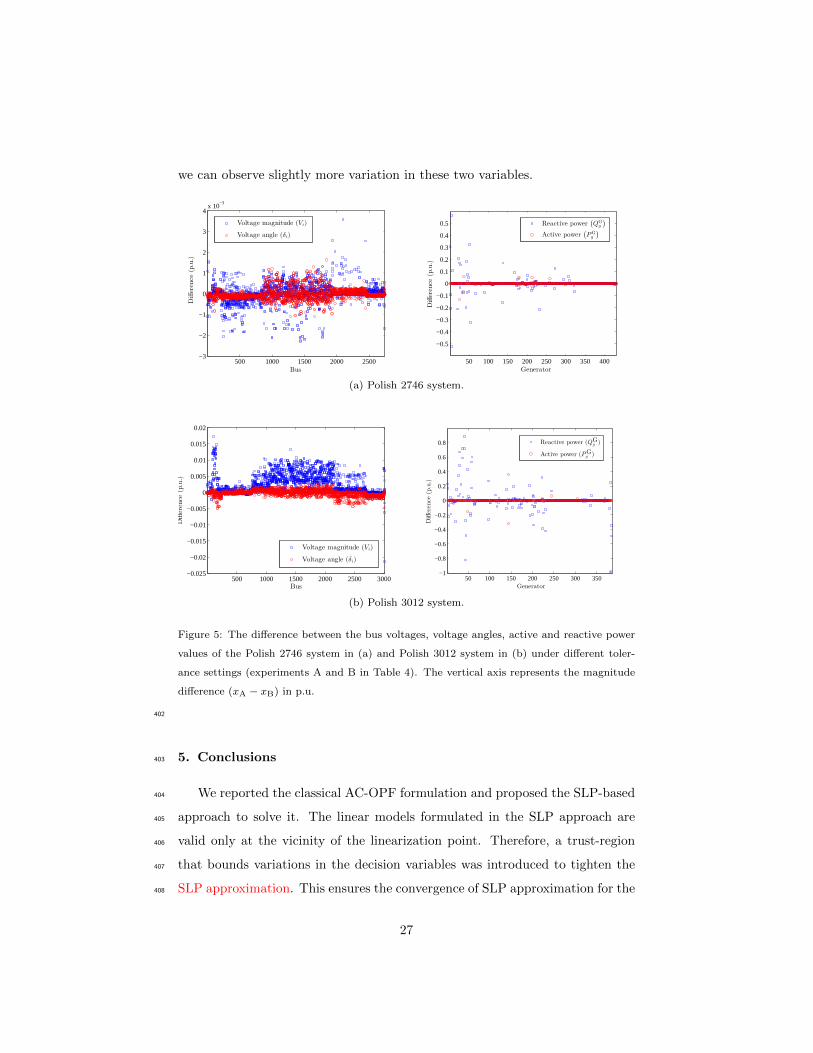
we can observe slightly more variation in these two variables.
500 1000 1500 2000 2500−3
−2
−1
0
1
2
3
4x 10
−3
Bus
Difference
(p.u.)
Voltage magnitude (Vi)
Voltage angle (δi)
50 100 150 200 250 300 350 400
−0.5
−0.4
−0.3
−0.2
−0.1
0
0.1
0.2
0.3
0.4
0.5
Generator
Difference
(p.u.)
Reactive power(
QGg
)
Active power(
PGg
)
(a) Polish 2746 system.
500 1000 1500 2000 2500 3000−0.025
−0.02
−0.015
−0.01
−0.005
0
0.005
0.01
0.015
0.02
Bus
Difference
(p.u.)
Voltage magnitude (Vi)
Voltage angle (δi)
50 100 150 200 250 300 350−1
−0.8
−0.6
−0.4
−0.2
0
0.2
0.4
0.6
0.8
Generator
Difference
(p.u.)
Reactive power (QGg)
Active power (PGg)
(b) Polish 3012 system.
Figure 5: The difference between the bus voltages, voltage angles, active and reactive power
values of the Polish 2746 system in (a) and Polish 3012 system in (b) under different toler-
ance settings (experiments A and B in Table 4). The vertical axis represents the magnitude
difference (xA − xB) in p.u.
402
5. Conclusions403
We reported the classical AC-OPF formulation and proposed the SLP-based404
approach to solve it. The linear models formulated in the SLP approach are405
valid only at the vicinity of the linearization point. Therefore, a trust-region406
that bounds variations in the decision variables was introduced to tighten the407
SLP approximation. This ensures the convergence of SLP approximation for the408
27
OPF problem (referred to as TR-SLP in this work). In addition, we also pro-409
posed the feasibility restoration phase based on the original nonlinear constraints410
to quickly locate a feasible point when the SLP approximation is infeasible. Re-411
sults show that our TR-SLP approach outperforms KNITRO, IPOPT and a412
recently reported SLP method based on penalty reformulations [6] in terms of413
computational time.414
We also used two generic starting point strategies (flat and DC warm start)415
and the OPF results on IEEE and Polish systems demonstrated the capability416
of TR-SLP to locate good local optimal solutions. It was observed, with these417
two starting strategies, in some cases, TR-SLP converges to a better solution418
than KNITRO-MS. It would be interesting to develop and study good starting419
point strategies for TR-SLP in future.420
Acknowledgement421
We acknowledge support from the International Center of Energy Research422
(ICER), established by Nanyang Technological University, Singapore and Tech-423
nische Universitat Munchen, Germany. We also acknowledge support from the424
National Research Foundation (NRF), Prime Minister’s Office, Singapore under425
its Campus for Research Excellence and Technological Enterprise (CREATE)426
programme.427
References428
[1] F. Capitanescu, J. M. Ramos, P. Panciatici, D. Kirschen, A. M. Marcolini,429
L. Platbrood, L. Wehenkel, State-of-the-art, challenges, and future trends430
in security constrained optimal power flow, Electric Power Systems Re-431
search 81 (8) (2011) 1731 – 1741.432
[2] F. Capitanescu, Critical review of recent advances and further develop-433
ments needed in ac optimal power flow, Electric Power Systems Research434
136 (2016) 57 – 68.435
28
[3] J. Lavaei, S. H. Low, Zero duality gap in optimal power flow problem, IEEE436
Transactions on Power Systems 27 (1) (2012) 92–107.437
[4] W. A. Bukhsh, A. Grothey, . I. M. McKinnon, P. A. Trodde, Local solutions438
of the optimal power flow problem, IEEE Transactions on Power Systems439
28 (4) (2013) 4780–4788.440
[5] B. Stott, O. Alsac, Optimal power flow−Basic requirements for real-life441
problems and their solutions, in: SEPOPE XII Symposium, Rio de Janeiro,442
Brazil, 2012.443
[6] A. Castillo, P. Lipka, J-P. Watson, S. S. Oren, R. P. O’Neill, A successive444
linear programming approach to solving the IV-ACOPF, IEEE Transac-445
tions on Power Systems 31 (4) (2016) 2752–2763.446
[7] S. Mhanna, G. Verbi, A. C. Chapman, Tight LP approximations for the447
optimal power flow problem, in: 2016 Power Systems Computation Con-448
ference (PSCC), 2016, pp. 1–7.449
[8] J. Horsch, H. Ronellenfitsch, D. Witthaut, T. Brown, Linear optimal power450
flow using cycle flows, Electric Power Systems Research 158 (2018) 126–135.451
[9] A. Garces, A quadratic approximation for the optimal power flow in power452
distribution systems, Electric Power Systems Research 130 (2016) 222–229.453
[10] D. Phan, J. Kalagnanam, Some efficient methods for solving the security-454
constrained optimal power flow problem, IEEE Transactions on Power Sys-455
tems 29 (2) (2014) 863–872.456
[11] F. Capitanescu, L. Wehenkel, Experiments with the interior-point method457
for solving large scale optimal power flow problems, Electric Power Systems458
Research 95 (2013) 276–283.459
[12] V. H. Quintana, G. L. Torres, J. Medina-Palomo, Interior-point methods460
and their applications to power systems: a classification of publications461
29
and software codes, IEEE Transactions on Power Systems 15 (1) (2000)462
170–176.463
[13] R. A. Jabr, A primal-dual interior-point method to solve the optimal power464
flow dispatching problem, Optimization and Engineering 4 (4) (2003) 309–465
336.466
[14] S. Frank, I. Steponavice, S. Rebennack, Optimal power flow: a biblio-467
graphic survey I, Energy Systems 3 (3) (2012) 221–258.468
[15] X. Bai, H. Wei, K. Fujisawa, Y. Wang, Semidefinite programming for op-469
timal power flow problems, International Journal of Electrical Power and470
Energy Systems 30 (6-7) (2008) 383–392.471
[16] H. Hijazi, C. Coffrin, P. V. Hentenryck, Polynomial SDP cuts for optimal472
power flow, in: 2016 Power Systems Computation Conference (PSCC),473
2016, pp. 1–7.474
[17] S. H. Low, Convex relaxation of optimal power flow-Part I: Formulations475
and equivalence, IEEE Transactions on Control of Network Systems 1 (1)476
(2014) 15–27.477
[18] S. H. Low, Convex relaxation of optimal power flow-Part II: Exactness,478
IEEE Transactions on Control of Network Systems 1 (2) (2014) 177–189.479
[19] R. Madani, S. Sojoudi, J. Lavaei, Convex relaxation for optimal power480
flow problem: Mesh networks, IEEE Transactions on Power Systems 30 (1)481
(2015) 199–211.482
[20] B. Kocuk, S. S. Dey, Xu. A. Sun, Inexactness of SDP relaxation and valid483
inequalities for optimal power flow, IEEE Transactions on Power Systems484
31 (1) (2016) 642–651.485
[21] C. Coffrin, H. L. Hijazi, P. V. Hentenryck, The QC relaxation: A theoretical486
and computational study on optimal power flow, IEEE Transactions on487
Power Systems 31 (4) (2016) 3008–3018.488
30

[22] M. Farivar, S. H. Low, Branch flow model: Relaxations and489
convexification−Part I, IEEE Transactions on Power Systems 28 (3) (2013)490
2554–2564.491
[23] M. Farivar, S. H. Low, Branch flow model: Relaxations and492
convexification−Part II, IEEE Transactions on Power Systems 28 (3) (2013)493
2565–2572.494
[24] H. Gao, J. Liu, L. Wang, Y. Liu, Cutting planes based relaxed optimal495
power flow in active distribution systems, Electric Power Systems Research496
143 (2017) 272–280.497
[25] Q. Zhijun, Y. Hou, Y. Chen, Convex envelopes of optimal power flow with498
branch flow model in rectangular form, IEEE Proceedings of Power and499
Energy Society General Meeting, Denver, CO (2015) 1–5.500
[26] D. Li, X. Li, Decomposition-based global optimization for optimal design of501
power distribution systems, 55th IEEE Proceedings of Control and Decision502
Conference, Las Vegas, USA (2016) 3265–3270.503
[27] Z. Yang, H. Zhong, Q. Xia, A. Bose, C. Kang, Optimal power flow based on504
successive linear approximation of power flow equations, IET Generation,505
Transmission Distribution 10 (14) (2016) 3654–3662.506
[28] A. Wachter, L. T. Biegler, On the implementation of a primal-dual interior507
point filter line search algorithm for large-scale nonlinear programming,508
Mathematical Programming 106 (1) (2006) 25–57.509
[29] R. H. Byrd, J. Nocedal, R. A. Waltz, KNITRO: An integrated package for510
nonlinear optimization, Springer, 2006.511
[30] S. Pajic, K. A. Clements, Power system state estimation via globally con-512
vergent methods, IEEE Transactions on Power Systems 20 (4) (2005) 1683–513
1689.514
31
[31] W. Min, L. Shengsong, A trust region interior point algorithm for optimal515
power flow problems, International Journal of Electrical Power and Energy516
Systems 27 (4) (2005) 293–300.517
[32] A. A. Sousa, G. L. Torres, C. A. Canizares, Robust optimal power flow518
solution using trust region and interior-point methods, IEEE Transactions519
on Power Systems 26 (2) (2011) 487–499.520
[33] W. Sheng, K. Liu, S. Cheng, Optimal power flow algorithm and analysis521
in distribution system considering distributed generation, IET Generation,522
Transmission and Distribution 8 (2) (2014) 261–272.523
[34] R. H. Byrd, Nicholas I.M. Gould, J. Nocedal, R. A. Waltz, An algorithm for524
nonlinear optimization using linear programming and equality constrained525
subproblems, Mathematical Programming 100 (1) (2004) 27–48.526
[35] R. D. Zimmerman, C. E. Murillo-Sanchez, R. J. Thomas, MATPOWER:527
Steady-state operations, planning, and analysis tools for power systems528
research and education, IEEE Transactions on Power Systems 26 (1) (2011)529
12–19.530
[36] The IBM Corp., CPLEX Version 12.6.3, New York, US, 2016.531
32


![Sequential Bayesian Sparse Signal Reconstruction …prior information using linear MMSE reconstruction. Here, we extend the Bayesian approach [13], [14], [15] to sequential Maximum](https://static.fdocuments.net/doc/165x107/5fd55d7c4d7fd26d021e4317/sequential-bayesian-sparse-signal-reconstruction-prior-information-using-linear.jpg)

