![[MS-H264PF]: RTP Payload Format for H.264 Video Streams ...MS-H264PF].pdf · Real-Time Transport Protocol (RTP): A network transport protocol that provides end-to-end transport functions](https://static.fdocuments.net/doc/165x107/5e8a7ea859c3b27da162b7e0/ms-h264pf-rtp-payload-format-for-h264-video-streams-ms-h264pfpdf-real-time.jpg)
A TRANSPORT PROTOCOL FOR DEDICATED END …mv/MSthesis/anant-thesis.pdfA TRANSPORT PROTOCOL FOR...
81
A TRANSPORT PROTOCOL FOR DEDICATED END-TO-END CIRCUITS A Thesis Presented to the faculty of the School of Engineering and Applied Science University of Virginia In Partial Fulfillment of the requirements for the Degree Master of Science Computer Engineering by Anant P. Mudambi January 2006
Transcript of A TRANSPORT PROTOCOL FOR DEDICATED END …mv/MSthesis/anant-thesis.pdfA TRANSPORT PROTOCOL FOR...

A TRANSPORT PROTOCOLFOR
DEDICATED END-TO-END CIRCUITS
A Thesis
Presented to
the faculty of the School of Engineering and Applied Science
University of Virginia
In Partial Fulfillment
of the requirements for the Degree
Master of Science
Computer Engineering
by
Anant P. Mudambi
January 2006

APPROVAL SHEET
This thesis is submitted in partial fulfillment of the requirements for the degree of
Master of Science
Computer Engineering
Anant P. Mudambi
This thesis has been read and approved by the examining committee:
Malathi Veeraraghavan (Advisor)
Marty A. Humphrey (Chair)
Stephen G. Wilson
Accepted for the School of Engineering and Applied Science:
Dean, School of Engineering and Applied Science
January 2006

Abstract
E-science projects involving geographically distributed data sources, computing resources and sci-
entists, have special networking requirements such as a steady throughput and deterministic behav-
ior. The connectionless Internet model is not well-suited to meet such requirements. Connection-
oriented networks that offer guaranteed-rate, dedicated circuits have been proposed to meet the
high-end networking needs of distributed scientific research. In this work we describe the design
and implementation of a transport protocol for such dedicated circuits.
We present an initial user-space, UDP-based implementation called Fixed Rate Transport Proto-
col (FRTP). The constraints imposed by a user-space implementation led us to implement a lower-
overhead kernel-space solution that we call Circuit-TCP (C-TCP). The key feature of C-TCP is to
maintain a fixed sending rate, closely matched to the circuit rate, with the aim of achieving high
circuit utilization. We implemented C-TCP by modifying the Linux TCP/IP stack. Experimental
results on a wide-area circuit-switched testbed show that C-TCP is able to quickly utilize circuit
bandwidth and sustain a high data transfer rate.
iii

Acknowledgments
I would like to thank Prof. Malathi Veeraraghavan, for her advice and for keeping me on the right
track. I thank the members of the CHEETAH research group, Xuan, Xiangfei, Zhanxiang and
Xiuduan, for all their help.
Anil and Kavita, thank you for keeping me motivated. Finally, the biggest thank you to my
parents, for their incredible support and love.
iv

Contents
1 INTRODUCTION 1
2 BACKGROUND 3
2.1 Related Work . . . . . . . . . . . . . . . . . . . . . . . . . . . . . . . . . . . . . 3
2.1.1 TCP Enhancements . . . . . . . . . . . . . . . . . . . . . . . . . . . . . . 3
2.1.2 UDP-based Protocols . . . . . . . . . . . . . . . . . . . . . . . . . . . . . 5
2.1.3 Novel Protocols . . . . . . . . . . . . . . . . . . . . . . . . . . . . . . . . 5
2.2 End-host Factors that Affect Data Transfer Performance . . . . . . . . . . . . . . . 6
2.2.1 Memory and I/O bus usage . . . . . . . . . . . . . . . . . . . . . . . . . . 6
2.2.1.1 Zero-copy Networking . . . . . . . . . . . . . . . . . . . . . . 7
2.2.2 Protocol Overhead . . . . . . . . . . . . . . . . . . . . . . . . . . . . . . 8
2.2.3 Disk Access . . . . . . . . . . . . . . . . . . . . . . . . . . . . . . . . . . 9
2.2.4 Process scheduling . . . . . . . . . . . . . . . . . . . . . . . . . . . . . . 10
2.3 CHEETAH Network . . . . . . . . . . . . . . . . . . . . . . . . . . . . . . . . . 11
2.3.1 Components of CHEETAH . . . . . . . . . . . . . . . . . . . . . . . . . . 11
2.3.2 Features of a CHEETAH Network . . . . . . . . . . . . . . . . . . . . . . 12
2.3.3 The CHEETAH Testbed . . . . . . . . . . . . . . . . . . . . . . . . . . . 13
2.3.4 End-host Software Support for CHEETAH . . . . . . . . . . . . . . . . . 14
3 UDP-BASED TRANSPORT PROTOCOL 16
3.1 SABUL Overview . . . . . . . . . . . . . . . . . . . . . . . . . . . . . . . . . . . 17
3.1.1 SABUL Implementation . . . . . . . . . . . . . . . . . . . . . . . . . . . 18
v
Contents vi
3.2 Modifications to SABUL : FRTP . . . . . . . . . . . . . . . . . . . . . . . . . . . 21
3.2.1 Problems with the FRTP Implementation . . . . . . . . . . . . . . . . . . 22
3.2.2 Possible Solutions . . . . . . . . . . . . . . . . . . . . . . . . . . . . . . 24
4 TCP-BASED SOLUTION 27
4.1 Transmission Control Protocol - A Primer . . . . . . . . . . . . . . . . . . . . . . 27
4.1.1 Error Control . . . . . . . . . . . . . . . . . . . . . . . . . . . . . . . . . 28
4.1.2 Flow Control . . . . . . . . . . . . . . . . . . . . . . . . . . . . . . . . . 29
4.1.3 Congestion Control . . . . . . . . . . . . . . . . . . . . . . . . . . . . . . 29
4.1.4 Self Clocking . . . . . . . . . . . . . . . . . . . . . . . . . . . . . . . . . 31
4.2 Reasons for Selecting TCP . . . . . . . . . . . . . . . . . . . . . . . . . . . . . . 32
4.3 Circuit-TCP Design . . . . . . . . . . . . . . . . . . . . . . . . . . . . . . . . . . 34
4.3.1 Connection Establishment . . . . . . . . . . . . . . . . . . . . . . . . . . 34
4.3.2 Congestion Control . . . . . . . . . . . . . . . . . . . . . . . . . . . . . . 34
4.3.3 Multiplexing . . . . . . . . . . . . . . . . . . . . . . . . . . . . . . . . . 35
4.3.4 Flow Control . . . . . . . . . . . . . . . . . . . . . . . . . . . . . . . . . 36
4.3.5 Error Control . . . . . . . . . . . . . . . . . . . . . . . . . . . . . . . . . 36
4.4 C-TCP Implementation . . . . . . . . . . . . . . . . . . . . . . . . . . . . . . . . 37
4.4.1 Web100 . . . . . . . . . . . . . . . . . . . . . . . . . . . . . . . . . . . . 38
4.4.2 Implementation Details . . . . . . . . . . . . . . . . . . . . . . . . . . . . 39
4.5 Experimental Results . . . . . . . . . . . . . . . . . . . . . . . . . . . . . . . . . 41
4.5.1 Utility of Disabling Slow Start . . . . . . . . . . . . . . . . . . . . . . . . 42
4.5.2 Sustained Data Transfer . . . . . . . . . . . . . . . . . . . . . . . . . . . 44
4.5.2.1 Reno-TCP Performance . . . . . . . . . . . . . . . . . . . . . . 46
4.5.2.2 BIC-TCP Performance . . . . . . . . . . . . . . . . . . . . . . 46
4.5.2.3 C-TCP Performance . . . . . . . . . . . . . . . . . . . . . . . . 47
5 CONTROL-PLANE FUNCTIONS 49
5.1 Selecting the Circuit Rate . . . . . . . . . . . . . . . . . . . . . . . . . . . . . . . 49

Contents vii
5.2 Setting up the Circuit . . . . . . . . . . . . . . . . . . . . . . . . . . . . . . . . . 53
6 CONCLUSIONS 56
6.1 Conclusions . . . . . . . . . . . . . . . . . . . . . . . . . . . . . . . . . . . . . . 56
6.1.1 Transport Protocol Design for Dedicated Circuits . . . . . . . . . . . . . . 56
6.1.2 Transport Protocol Implementation . . . . . . . . . . . . . . . . . . . . . 57
6.2 Future Work . . . . . . . . . . . . . . . . . . . . . . . . . . . . . . . . . . . . . . 57
A DISK WRITE RATE ESTIMATION 59
A.1 How Linux Handles Disk Writes . . . . . . . . . . . . . . . . . . . . . . . . . . . 59
A.2 Benchmark Results . . . . . . . . . . . . . . . . . . . . . . . . . . . . . . . . . . 62
Bibliography 66

List of Figures
2.1 Memory I/O bus usage . . . . . . . . . . . . . . . . . . . . . . . . . . . . . . . . 7
2.2 CHEETAH experimental testbed . . . . . . . . . . . . . . . . . . . . . . . . . . . 13
2.3 Architecture of CHEETAH end-host software . . . . . . . . . . . . . . . . . . . . 15
3.1 Architecture of a generic UDP-based protocol . . . . . . . . . . . . . . . . . . . . 17
3.2 Need for receiver flow control . . . . . . . . . . . . . . . . . . . . . . . . . . . . 24
4.1 TCP self clocking . . . . . . . . . . . . . . . . . . . . . . . . . . . . . . . . . . . 32
4.2 Congestion control in the control plane . . . . . . . . . . . . . . . . . . . . . . . . 35
4.3 Structure of the Web100 stack . . . . . . . . . . . . . . . . . . . . . . . . . . . . 38
4.4 Maximum buffer space required for a C-TCP burst . . . . . . . . . . . . . . . . . 41
4.5 Testbed configuration for C-TCP tests . . . . . . . . . . . . . . . . . . . . . . . . 42
4.6 TCP and C-TCP comparison for different transfer sizes . . . . . . . . . . . . . . . 43
4.7 Start-up behavior of TCP and C-TCP . . . . . . . . . . . . . . . . . . . . . . . . . 44
4.8 Throughput and RTT using Reno-TCP . . . . . . . . . . . . . . . . . . . . . . . . 46
4.9 Throughput and RTT using BIC-TCP . . . . . . . . . . . . . . . . . . . . . . . . 47
4.10 Throughput and RTT using C-TCP . . . . . . . . . . . . . . . . . . . . . . . . . . 48
5.1 Throughput variability of disk-to-disk transfers . . . . . . . . . . . . . . . . . . . 50
5.2 Trade-off between circuit utilization and delay . . . . . . . . . . . . . . . . . . . . 51
viii

List of Tables
5.1 xdd benchmark results on zelda4 . . . . . . . . . . . . . . . . . . . . . . . . . . . 52
5.2 Disk write rate (Mbps) for individual runs using 32 KB request sizes . . . . . . . . 52
A.1 End host configurations . . . . . . . . . . . . . . . . . . . . . . . . . . . . . . . . 63
A.2 Disk write rate results using xdd . . . . . . . . . . . . . . . . . . . . . . . . . . . 63
ix

List of Abbreviations
ACK Acknowledgement
AIMD Additive Increase Multiplicative Decrease
API Application Programming Interface
AQM Active Queue Management
BDP Bandwidth Delay Product
BIC-TCP Binary Increase Congestion control TCP
CHEETAH Circuit-switched High-speed End-to-End Transport ArcHitecture
COW Copy On Write
C-TCP Circuit TCP
cwnd congestion window
DMA Direct Memory Access
DNS Domain Name Service
DRAGON Dynamic Resource Allocation via GMPLS Optical Networks
FAST Fast AQM Scalable TCP
FRTP Fixed Rate Transport Protocol
GbE Giga bit Ethernet
Gbps Giga bits per second
GB Giga Byte
GMPLS Generalized Multiprotocol Label Switching
x

List of Abbreviations xi
HS-TCP HighSpeed TCP
I/O Input/Output
IP Internet Protocol
KB Kilo Byte
LAN Local Area Network
LMP Link Management Protocol
Mbps Mega bits per second
MB Mega Byte
MSPP Multi-Service Provisioning Platform
MTU Maximum Transmission Unit
NAK Negative ACK
NETBLT Network Blast Transfer
NIC Network Interface Card
OC Optical Carrier
OCS Optical Connectivity Service
OS Operating System
OSPF Open Shortest Path First
RBUDP Reliable Blast UDP
RED Random Early Detect
RSVP-TE Resource Reservation Protocol
RTO Retransmission Time-out
RTT Round Trip Time
rwnd receiver advertised window
SABUL Simple Available Bandwidth Utilization Library
SACK Selective ACK
SONET Synchronous Optical Network
ssthresh slow start threshold
TCP Transmission Control Protocol

List of Abbreviations xii
TDM Time Division Multiplexing
TSI Terascale Supernova Initiative
UDP User Datagram Protocol
UDT UDP-based Data Transfer protocol
XCP eXplicit Control Protocol

Chapter 1
INTRODUCTION
Many fields of research require significant computing resources to conduct simulations and/or to
analyze large amounts of data. Large data sets collected by remote instruments may need to be
processed. The SETI@home project [2], which uses data collected by the National Astronomy
and Ionospheric Center’s radio telescope in Arecibo, Peru, is one such example. The telescope
generates about 35 GB of data per day that is stored in removable tapes and physically transported
to the server in Berkeley, California. In some cases, computations generate massive amounts of
output that has to be distributed to scientists who are physically at a distance from the computation
resource. For instance, the Terascale Supernova Initiative (TSI) project involves simulations run on
supercomputers at the Oak Ridge National Laboratory (ORNL), the results of which are used by
physicists at remote sites like the North Carolina State University (NCSU).
Networks connecting the data generation point, the computation resource and the scientists’
workplace make collabarative e-science much more practical. The large amounts of data involved
and, in some cases (e.g., real-time visualization), stringent delay/jitter requirements make it nec-
essary to use networks with large bandwidths and deterministic behavior. E-science applications
require high, constantly available bandwidth for their data transfer needs. It is difficult to provide
such rate-guaranteed services in packet-switched, connectionless networks, such as the present-day
Internet. This is because of the possibility of a large number of simultaneous flows competing for
the available network capacity. Therefore, the use of connection-oriented, dedicated circuits has
been proposed as a solution. Many research groups are implementing testbeds and the supporting
1

Chapter 1. INTRODUCTION 2
software to show the feasibility of such a solution.
The problem addressed in this thesis is the design of a transport protocol for dedicated circuits.
Many of the assumptions on which traditional transport protocols for packet-switched networks
are based need to be examined. For instance, the possibility of losses due to network buffer over-
flows makes congestion control an important function on connectionless networks. On connection-
oriented networks, because network resources are reserved for each data transfer, the end points of
the transfer have more control over whether or not network buffers will overflow. By maintaining
a data transfer rate that is matched to the reserved circuit’s rate the need for congestion control
can be eliminated. On the other hand, a transport layer function such as flow control is needed on
both connectionless and connection-oriented networks because it addresses a problem that network
resource reservation does not solve.
Our approach is to design the transport protocol under the assumption that resources are re-
served for a data transfer’s exclusive use. The transport protocol should not have any “features”
that leave the reserved circuit unutilized. We implemented the transport protocol and tested it on a
wide-area, connection-oriented network testbed. This protocol is called Circuit-TCP (C-TCP).
The rest of this thesis is organized as follows. Chapter 2 provides background information on
previous work in this area as well as issues that affect the design and performance of our transport
protocol. In Chapter 3, we describe the Fixed Rate Transport Protocol (FRTP) that was implemented
in the user space over UDP. The shortcomings of a user space impementation are pointed out.
Chapter 4 describes the design and implementation of C-TCP, our kernel space transport protocol
based on TCP. Experimental results over a testbed are used to compare C-TCP with TCP over
dedicated circuits. In Chapter 5 the control plane issues of determining the circuit rate and then
setting up the circuit are considered. The conclusions of this work are presented in Chapter 6.

Chapter 2
BACKGROUND
In this chapter we first look at other work that has been done in the development of transport pro-
tocols for high-performance networks. Next we point out some of the factors that play a significant
role in achieving high throughput on dedicated circuits. Many of these are end-host issues that we
discovered while implementing our transport protocol. This work has been conducted as a part
of the Circuit-switched High-speed End-to-End Transport ArcHitecture (CHEETAH) project. An
overview of CHEETAH is presented at the end of this chapter.
2.1 Related Work
There has been significant activity in developing transport protocols suitable for high-bandwidth
and/or high-delay networks. Even though very little of it is focussed explicitly towards dedicated
circuits there is enough of an overlap in the problems to justify a closer examination. High-
performance protocols can be classified as TCP enhancements, UDP-based and novel protocols.
Ease of deployment and familiarity with the sockets API to the TCP and UDP protocol stacks are
reasons for the popularity of TCP and UDP-based solutions.
2.1.1 TCP Enhancements
TCP is the most widely used reliable transport protocol on connectionless, packet-switched net-
works. We describe basic TCP operation in Chapter 4. It is designed to work under a wide range
3

Chapter 2. BACKGROUND 4
of conditions and this makes a few of its design decisions non-optimal for high-speed networks.
In recent years a number of protocol extensions to TCP have been proposed and implemented to
address this issue. Selective acknowledgements (SACKs) [27,16] have been proposed to deal more
efficiently with multiple losses in a round trip time (RTT) [13]. TCP uses cumulative acknowl-
edgements (ACKs) which means a data byte is not ACKed unless all data earlier in the sequence
space has been received successfully. SACKs inform the sender about out-of-sequence data already
received and help prevent unnecessary retransmissions. Two protocol extensions— timestamps op-
tion and window scaling— were proposed in [22]. The timestamps option field in a data packet’s
TCP header is filled in by a sender and echoed back in the corresponding ACK. It serves two pur-
poses. First, the timestamp can be used to estimate the round trip time more accurately and more
often. This gives the sender a better value for retransmission timeout (RTO) computation. Second,
the timestamp in a received packet can be used to prevent sequence number wraparound. The TCP
header has a 16-bit field for the window size, which limits the window size to 64 KB. This is insuf-
ficient for high-bandwidth, high-delay networks. The window scaling option allows a scaling factor
to be chosen during connection establishment. Subsequent window advertisements are right shifted
by the selected scaling factor. Scaling factors of upto 14 are allowed, thus by using this option a
window size of upto 1 GB can be advertised.
Standard TCP (also called Reno TCP) has been found wanting in high-bandwidth, high-delay
environments, mainly due to its congestion control algorithm. TCP’s Additive Increase Multi-
plicative Decrease (AIMD) algorithm is considered too slow in utilizing available capacity and too
drastic in cutting back when network congestion is inferred. Modifications to the TCP conges-
tion control algorithm have led to the development of HighSpeed TCP [14], Scalable TCP [25],
FAST [23], and BIC-TCP [39], among others. Standard TCP requires unrealistically low loss rates
to achieve high throughputs. HighSpeed TCP is a proposed change to the TCP AIMD parameters
that allows a TCP connection to achieve high sending rates under more realistic loss conditions.
Scalable TCP also proposes modified AIMD parameters that speed up TCP’s recovery from loss.
FAST infers network congestion and adjusts its window size based on queueing delays rather than
loss. BIC-TCP (BIC stands for Binary Increase Congestion control) is a new congestion control

Chapter 2. BACKGROUND 5
algorithm that scales well to high bandwidth (i.e., it can achieve a high throughput at reasonable
packet loss rates) and is TCP-friendly (i.e., when the loss rate is high its performance is the same
as standard TCP’s). In addition, unlike HighSpeed or Scalable TCP, BIC-TCP’s congestion control
is designed such that two flows with different RTTs share the available bandwidth in a reasonably
fair manner.
2.1.2 UDP-based Protocols
To overcome the shortcomings of TCP, many researchers have implemented protocols over UDP by
adding required functionality, such as reliability, in the user space. The most common model is to
use UDP for the data transfer and a separate TCP or UDP channel for control traffic. SABUL [18],
Tsunami, Hurricane [38], and RBUDP [20] use a TCP control channel and UDT [19] uses UDP
for both data and control channels. The advantage of these solutions is that their user-space imple-
mentation makes deployment easy. At the same time, there are some limitations that arise because
these protocols are implemented in the user-space. In Chapter 3, we describe SABUL. Our attempt
at modifying SABUL to implement a transport protocol for dedicated circuits and the shortcomings
of a user-space transport protocol implementation are also pointed out.
2.1.3 Novel Protocols
Some novel protocols designed exclusively for high-performance data transfer have also been pro-
posed. The eXplicit Control Protocol (XCP) [24] was proposed to solve TCP’s stability and effi-
ciency problems. By separating link utilization control from fairness control, XCP is able to make
more efficient use of network resources in a fair manner. XCP’s requirement of multi-bit congestion
signals from the network makes it harder to deploy since routers in the network need to be modified.
NETBLT [10] was proposed for high-speed bulk data transfer. It provides reliable data transfer by
sending blocks of data in a lock-step manner. This degrades bandwidth utilization while the sender
awaits an acknowledgement (ACK) for each block.

Chapter 2. BACKGROUND 6
2.2 End-host Factors that Affect Data Transfer Performance
Setting up a dedicated circuit involves resource reservation in the network. Depending on the
network composition, the resources reserved could be wavelengths, ports on a switch or time slots.
Ideally, we would like to fully use the reserved resources for exactly the time required to complete
the transfer. During the implementation of our transport protocol, we found that there are many
factors that make it hard to achieve this ideal. In this section we list a few of these factors that
impact the performance of transport protocol implementations.
2.2.1 Memory and I/O bus usage
First, consider an application that uses the transport protocol to carry out a file transfer. At the
sending end, the application has to
1. Read data from the disk, e.g. by invoking a read system call.
2. Send the data out on the network, e.g. by invoking a send system call.
There are two types of overhead in carrying out these operations. The system calls involve the over-
head of saving the process registers on stack before the system call handler is invoked. Secondly,
the two steps shown above could involve multiple passes over the memory and I/O bus. This is
illustrated in Figure 2.1(a). The figure shows the bus operations involved in moving data from the
disk to user space buffers (step 1 above), and from the user space buffer to kernel network buffers
(part of step 2). To avoid having to access the disk each time, for multiple accesses to a chunk of
data, the operating system caches recently accessed disk data in memory. This cache is called the
page cache, and direct memory access (DMA) is used for transfers between the page cache and the
disk (operation I in Figure 2.1(a)). Two passes over the memory bus are needed to transfer the data
from the page cache to the user space buffer (operation II). To send data out to the network, it is
again copied from the user space buffer to kernel network buffers (operation III). We do not show
the transfer from the kernel network buffer to the NIC, which is the final step in getting data out
into the network. For data transfers using TCP sockets on Linux, the sendfile system call can be

Chapter 2. BACKGROUND 7
PROCESSOR
MEMORY
PAGE
CACHE
I
II
III
NICHARD DISK
USER-SPACE
KERNEL-SPACE MEMORY
(a) Using read and send
PROCESSOR
MEMORY
PAGE
CACHE
HARD DISKNIC
KERNEL-SPACE
MEMORY
USER-SPACE
(b) Using sendfile
Figure 2.1: Memory I/O bus usage
used to cut down the number of passes over the memory bus to three. As shown in Figure 2.1(b),
sendfile copies data directly from the page cache to the kernel network buffers, thus avoiding the
copy to user space and back. In addition, sendfile needs to be invoked just once for a single file, so
the overhead of making a system call is paid only once per file.
2.2.1.1 Zero-copy Networking
Other methods for avoiding the copy from user-space memory to kernel-space memory have been
proposed. Such methods are known by the common term zero-copy networking. For a classification
of zero-copy schemes see [7]. The zero in zero-copy networking indicates that there is no memory-
to-memory copy involved in the transfer of data between a user space buffer and the network. So,
in Figure 2.1(a), a zero-copy scheme would eliminate memory-to-memory copies after operation
II. How the data got into the user- or kernel-space buffer in the first place, and whether that required
a copy is not considered. Zero-copy schemes can be supported if an application interacts directly
with the NIC without passing through the kernel, or if the buffers are shared between user and
kernel space, rather than being copied. For an application to directly read from and write to the NIC
buffer, protocol procesing has to be done on the NIC. At the sender, buffers can be shared between
the application and the kernel if the application can guarantee that a buffer that has not yet been
transmitted will not be overwritten. One way to ensure this would be if the system call invoked to

Chapter 2. BACKGROUND 8
send some data returns only after all of that data has been successfully transmitted. Since a reliable
transport protocol can consider a buffer to have been successfully transmitted only when all of the
data in that buffer has successfully reached the intended receiver, the application may need to wait
a while before it can reuse a buffer. An interesting alternative is to mark the buffer as copy-on-write
(COW), so that the contents of the buffer are copied to a separate buffer if and when the application
tries to overwrite it. Implementation of send-side zero-copy schemes for different operating systems
are described in [28].
Now consider the steps at a receiver. A receiver performs the steps shown in Figure 2.1(a) in
reverse order (there is no sendfile equivalent for the receiver). One way to implement zero-copy
on the receiver is to change the page table of the application process when it issues a recv system
call. This is called page flipping in [28]. Page flipping works only if the NIC separates the packet
payload and header, if the packet payload is an exact multiple of the page size and if the buffer
provided by the application is aligned to page boundaries. Because of these requirements there has
been little effort to implement such a scheme.
Several factors that influence communication overhead are presented in [33]. The memory and
I/O bus usage for schemes with different kernel and interface hardware support are compared. For
instance, the author shows how, by using DMA, NIC buffering and checksum offload, the number
of passes over the bus can be reduced from six to one.
2.2.2 Protocol Overhead
Apart from the memory and I/O bus, the other main end host resource that could become a bottle-
neck is processor cycles. TCP/IP, being the most widely used protocol stack, has received attention
in this regard. In [9] the processing overhead of TCP/IP is estimated and the authors’ conclusion
is that with a proper implementation, TCP/IP can sustain high throughputs efficiently. More recent
work presented in [17] takes into consideration the OS and hardware support that a TCP implemen-
tation will require.
The overhead of a transport layer protocol can be divided into two categories: per-packet costs
and per-byte costs [9, 28, 6]. Per-packet costs include protocol processing (e.g., processing the

Chapter 2. BACKGROUND 9
sequence numbers on each packet in TCP) and interrupt processing. Per-byte costs are incurred
when data is copied or during checksum calculation.
Per-packet overhead can be reduced by reducing the number of packets handled during the
transfer. For a given transfer size, the number of packets can be reduced by using larger packets.
The maximum transmission unit (MTU) of the network constrains the packet size that an end host
can use. For instance, Ethernet imposes a 1500-byte limit on the IP datagram size. The concept
of jumbograms was introduced by Alteon Networks to allow Ethernet frames of upto 9000 bytes,
and many gigabit Ethernet NICs now support larger frame sizes. Larger packet sizes can decrease
protocol processing overhead as well as the overhead of interrupt processing. NICs interrupt the
processor on frame transmission and reception. An interrupt is costly for the processor because
the state of the currently running process has to be saved and an interrupt handler invoked to deal
with the interrupt. As interface rates increase to 1 Gbps and higher, interrupt overhead can become
significant. Many high-speed NICs support interrupt coalescing so that the processor is interrupted
for a group of transmitted or received packets, rather than for each individual packet.
Schemes to reduce per-byte costs involved in copying data over the memory I/O bus were
described in Section 2.2.1. Checksum calculation can be combined with a copy operation and
carried out efficiently in software. For instance, the sender could calculate the checksum when data
is being copied from the user-space buffer to the kernel-space buffer. Another way to reduce the
processor’s checksum calculation burden is to offload it to the interface card.
2.2.3 Disk Access
All the factors considered so far affect data transfer throughput. In designing a transport protocol
for dedicated circuits, not only does a high throughput have to be maintained, the circuit utilization
should also be high. Thus end host factors that cause variability in the throughput also need to
be considered. For disk-to-disk data transfers, disk access can limit throughput as well as cause
variability. The file system used can have an effect on disk access performance. The time to
physically move the disk read/write head to the area on the hard disk where the desired data resides,
called seek time, is a major component of the disk access latency. File accesses tend to be sequential,

Chapter 2. BACKGROUND 10
so a file system that tries to keep all parts of a file clustered together on the hard disk would perform
better than one in which a file is broken up into small pieces spread all over the hard disk.
At the sender, data needs to be read from the disk to memory. System calls to do this are
synchronous. When the system call returns successfully, the requested data is available in memory
for immediate use. Operating systems try to improve the efficiency of disk reads by reading in
more than the requested amount, so that some of the subsequent requests can be satisfied without
involving the disk hardware. At the data receiver, the system call to write to disk is asynchronous
by default. This means that when the system call returns it is not guaranteed that the data has been
written to disk; instead it could just be buffered in memory. Asynchronous writes are tailored to
make the common case of small, random writes efficient, since they allow the operating system
to schedule disk writes in an efficient manner. The operating system could reorder the writes to
minimize seeks. In Linux, for instance, data written to disk is actually copied to memory buffers
in the page cache and these buffers are marked dirty. Two kernel threads, bdflush and kupdate, are
responsible for flushing dirty buffers to disk. The bdflush kernel thread is activated when the number
of dirty buffers exceeds a threshold, and kupdate is activated whenever a buffer has remained dirty
too long. As a consequence of the kernel caching and delayed synchronization between memory
buffers and the disk, there can be significant variability in the conditions under which a disk write
system call operates.
2.2.4 Process scheduling
The final factor we consider is the effect of the process scheduler. All modern operating sys-
tems are multitasking. Processes run on the processor for short intervals of time and then either
relinquish the CPU voluntarily (e.g. if they block waiting for I/O) or are forcibly evicted by the
operating system if their time slot runs out. This gives users the impression that multiple processes
are running simultaneously. Multitasking, like packet-switched networking, tries to fairly divide up
a resource (processor cycles for multitasking; bandwidth for packet-switched networking) among
all contenders (multiple processes; multiple flows) for the resource. This behavior is at odds with
resource reservation in a connection-oriented network such as CHEETAH. If the degree of mul-

Chapter 2. BACKGROUND 11
titasking at an end host is high then a data transfer application may not get the processor cycles
required to fully use the reserved circuit. Even if the required number of free cycles are available,
the process scheduler might not be able to schedule the data transfer application in the monotonic
fashion required to send and receive data at the fixed circuit rate.
2.3 CHEETAH Network
CHEETAH, which stands for Circuit-switched High-speed End-to-End Transport ArcHitecture, is a
network architecture that has been proposed [37] to provide high-speed, end-to-end connectivity on
a call-by-call basis. Since the transport protocol proposed in this thesis is to be used over a dedicated
circuit through a CHEETAH network, in this section we provide a description of CHEETAH.
2.3.1 Components of CHEETAH
Many applications in the scientific computing domain require high throughput transfers with deter-
ministic behavior. A circuit-switched path through the network can meet such requirements better
than a packet-switched path. CHEETAH aims to bring the benefits of a dedicated circuit to an end-
user. In order to allow wide implementation, CHEETAH has been designed to build on existing
network infrastructure instead of requiring radical changes. Ethernet and SONET (Synchronous
Optical Network) are the most widely used technologies in local area networks (LANs) and wide
area networks (WANs) respectively. To take advantage of this, a CHEETAH end-to-end path con-
sists of Ethernet links at the edges and Ethernet-over-SONET links in the core. Multi-Service
Provisioning Platforms (MSPPs) are hardware devices that make such end-to-end paths possible.
MSPPs are capable of mapping between the packet-switched Ethernet domain and the time divi-
sion multiplexed (TDM) SONET domain. MSPPs are an important component of the CHEETAH
architecture for three reasons.
1. The end hosts can use common Ethernet NICs and do not need, for instance, SONET line
cards.
2. Many enterprises already have MSPPs deployed to connect to their ISP’s backbone network.

Chapter 2. BACKGROUND 12
3. Standard signaling protocols, as defined for Generalized Multiprotocol Label Switching
(GMPLS) networks, are (being) implemented in MSPPs. This is essential to support dynamic
call-by-call sharing in a CHEETAH network.
2.3.2 Features of a CHEETAH Network
One of the salient features of CHEETAH is that it is an add-on service to the existing packet-
switched service through the Internet. This means, firstly, that applications requiring CHEETAH
service can co-exist with applications for which a path through the packet-switched Internet is good
enough. Secondly, because network resources are finite, it is possible that an application’s request
for a dedicated circuit is rejected; in such cases, the Internet path provides an alternative so that
the application’s data transfer does not fail. To realize this feature, end hosts are equipped with an
additional NIC that is used exclusively for data transfer over a CHEETAH circuit.
To make the CHEETAH architecture scalable, the network resource reservation necessary to
set up an end-to-end circuit should be done in a distributed and dynamic manner. Standardized
signaling protocols that operate in a distributed manner, such as the hop-by-hop signaling in GM-
PLS protocols, are key to achieving scalability. CHEETAH uses RSVP-TE1 signaling in the control
plane. Dynamic circuit set up and tear down means that these operations are performed when (and
only when) required, as opposed to statically provisioning a circuit for a long period of time. Dy-
namic operation is essential for scalability because it allows the resources to be better utilized, thus
driving down costs. End-host applications that want to use a CHEETAH circuit are best-placed
to decide when the circuit should be set up or torn down. Therefore an end host connected to the
CHEETAH network runs signaling software that can be used by applications to attempt circuit set
up on a call-by-call basis.
With end-host signaling in place, applications that want to use a CHEETAH circuit can do so
in a dynamic manner. This leads to the question of whether, just because it can be done, a circuit
set up should be attempted for a given data transfer. In [37], analytical arguments are used to show
1Resource Reservation Protocol-Traffic Engineering. This is the signaling component of the GMPLS protocols, theother components being Link Management Protocol (LMP) and Open Shortest Path First-TE (OSPF-TE).

Chapter 2. BACKGROUND 13
that, for data transfers above a threshold size, transfer delay can be reduced by using a CHEETAH
circuit rather than an Internet path. It is also worth noting that there are situations in which the
overhead of circuit set up makes it advantageous to use a path through the Internet, although for
wide-area bulk data transfer a dedicated circuit invariably trumps an Internet path.
2.3.3 The CHEETAH Testbed
To study the feasibility of the CHEETAH concept, an experimental testbed has been set up. This
testbed extends between North Carolina State University (NCSU), Raleigh, NC, and Oak Ridge Na-
tional Laboratory (ORNL), Oak Ridge, TN and passes through the MCNC point-of-presence (PoP)
in Research Triangle Park, NC and the Southern Crossroads/Southern LambdaRail (SOX/SLR) PoP
in Atlanta, GA. The testbed layout is shown in Figure 2.2. In this testbed, the Sycamore SN16000
Intelligent Optical Switch is used as the MSPP. In the figure we show end hosts connected directly
or through Ethernet switches to the gigabit Ethernet card on the SN16000. The cross connect card
is configured through the control card to set up a circuit. The SN16000 has an implementation of
the GMPLS signaling protocol that follows the standard and has been tested for interoperability.
����������� ������� �� �� ��
����� � ����� �� ���
����� �"!���$#&%('
��) ���* ���+�,�-��#&.(/�/(/
!��10��( �
�,2�� 3(4&!��
�5�(�� ���(& ���(��� &� 6� ���
�7�8� � �+��� �� ���
�9�,����!�5�:#�%�'
�;) ��8* �����1�7� #6.�/(/�/
!��10��� �
< � � � � ��� 46� <
�5�(�� ���(& ���(��� &� 6� ���
�7�8� � �+��� �� ���
�9�,����!�5�:#�%�'
�;) ��8* �����1�7� #6.�/(/�/
!��10��� �
=>�$�?�$4����
�5���A@�B � 0
�5�(�C@DB �� 0
!"�>0��� � �?� � E 4��?�
Figure 2.2: CHEETAH experimental testbed

Chapter 2. BACKGROUND 14
The testbed has been designed to support the networking needs of the TSI project mentioned
at the beginning of this chapter. We present results of experiments conducted over this testbed in
Chapter 4.
2.3.4 End-host Software Support for CHEETAH
To allow applications to start using CHEETAH circuits, software support is required to make the
end hosts CHEETAH enabled. The architecture of the end-host software is shown in Figure 2.3.
The relevant components of the CHEETAH end-host software are shown inside a dotted box to
signify that the application could either interact with each component individually or make higher-
level calls that hide the details of the components being invoked. To be able to use a CHEETAH
circuit between two end hosts, both should support CHEETAH.
The Optical Connectivity Service (OCS) client allows applications to query whether a re-
mote host is on the CHEETAH network. OCS uses the Internet’s Domain Name Service (DNS)
to provide additional information such as the IP address of the remote end’s secondary NIC. As
mentioned earlier, depending on the situation, either a CHEETAH circuit or a path through the In-
ternet may be better for a particular transfer. The routing decision module takes measurements of
relevant network parameters (e.g., available bandwidth and average loss rate) and uses these along
with the parameters of a particular transfer (e.g., the file size and requested circuit rate) to decide
whether or not a CHEETAH circuit set up should be attempted. To achieve CHEETAH’s goal of
distributed circuit set up, an RSVP-TE signaling module runs on each end host. The RSVP-TE
module exchanges control messages with the enterprise MSPP to set up and tear down circuits.
These control messages are routed through the primary NIC over the Internet. The final software
component is the transport protocol module. Depending on whether a circuit or an Internet path
is being used, the transport protocol used will be C-TCP or TCP. In this thesis the focus will be on
the design, implementation and evaluation of C-TCP.
To end this chapter we mention some of the other projects focused on connection-oriented
networking for e-science projects. UltraScience Net [36] is a Department of Energy sponsored
research testbed connecting Atlanta, Chicago, Seattle and Sunnyvale. This network uses a central-

Chapter 2. BACKGROUND 15
������������
������� � ���� �� ��
����� �� � !��" # %$ �� ��&'�!��� �(� ��
# �*),+���-.��� � !���
-0/1�%���%/ �+0/2 �������34���$�� !
+0/�� 54��/ 67�8 �
�.!����������/ 67�8 �
39�:+.+
8 �" �!�/;��!
�.�47��%-<�!� =��/�> 39�:+.+
�0�����?�����
+0/�� 54��/ 67�8 �
�.!��(�������/ 67@8 �
Figure 2.3: Architecture of CHEETAH end-host software
ized scheme for the control-plane functions. Another effort is the Dynamic Resource Allocation via
GMPLS Optical Networks (DRAGON) project [12]. DRAGON uses GMPLS protocols to support
dynamic bandwidth provisioning.

Chapter 3
UDP-BASED TRANSPORT PROTOCOL
In Chapter 2 we mentioned a few protocols that are based on UDP. There are good reasons for
taking this approach:
• UDP provides the minimal functionality of a transport protocol. It transfers datagrams be-
tween two processes but makes no guarantees about their delivery. UDP’s minimalism leaves
no scope for anything to be taken out of its implementation. Thus a new protocol built over
UDP has to add extra (and only the required) functionality. The significance of this is that
these additions can be done in the user space, without requiring changes to the operating
system code. This makes UDP-based solutions as easy to use and portable as an application
program.
• The sockets API to the UDP and TCP kernel code is widely deployed and used. This makes
implementation easier and faster.
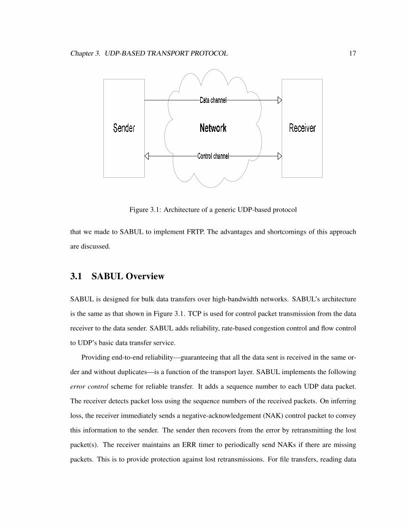
The basic design of all UDP-based protocols is similar and is shown in Figure 3.1. Data packets
are transferred using UDP sockets. A separate TCP or UDP channel is used to carry control pack-
ets. Control packets serve to add features to the data transfer not provided by UDP’s best-effort
service. We used the Simple Available Bandwidth Utilization Library (SABUL), a UDP-based data
transfer application, to implement the Fixed Rate Transport Protocol (FRTP). In this chapter we first
present an overview of the SABUL protocol and implementation. Then we describe the changes
16
Chapter 3. UDP-BASED TRANSPORT PROTOCOL 17
����������� ������ �����������������
���! �"$#%�'&�(*),+! - *.'&
/0+,"1+�(*)-+' ' 2.!&
Figure 3.1: Architecture of a generic UDP-based protocol
that we made to SABUL to implement FRTP. The advantages and shortcomings of this approach
are discussed.
3.1 SABUL Overview
SABUL is designed for bulk data transfers over high-bandwidth networks. SABUL’s architecture
is the same as that shown in Figure 3.1. TCP is used for control packet transmission from the data
receiver to the data sender. SABUL adds reliability, rate-based congestion control and flow control
to UDP’s basic data transfer service.
Providing end-to-end reliability—guaranteeing that all the data sent is received in the same or-
der and without duplicates—is a function of the transport layer. SABUL implements the following
error control scheme for reliable transfer. It adds a sequence number to each UDP data packet.
The receiver detects packet loss using the sequence numbers of the received packets. On inferring
loss, the receiver immediately sends a negative-acknowledgement (NAK) control packet to convey
this information to the sender. The sender then recovers from the error by retransmitting the lost
packet(s). The receiver maintains an ERR timer to periodically send NAKs if there are missing
packets. This is to provide protection against lost retransmissions. For file transfers, reading data

Chapter 3. UDP-BASED TRANSPORT PROTOCOL 18
from the disk for each retransmission is very expensive in time. Therefore, the sender keeps the
transmitted data in memory until it is acknowledged. A SABUL receiver periodically sends an ac-
knowledgement (ACK) control packet, acknowledging all packets received in-order. On receiving
an ACK, the sender can free the buffer space occupied by data that is confirmed to have been re-
ceived. In addition the SABUL sender has a timer that is reset each time a control packet is received.
If this timer (called the EXP timer) expires because no control information has been received, the
sender assumes that all unacknowledged packets have been lost and retransmits them.
SABUL uses a rate-based congestion control scheme. The sender modifies the sending rate
depending on the degree of congestion in the network. The SABUL receiver sends a periodic syn-
chronization (SYN) control packet containing the number of data packets received in the previous
SYN period. The sender uses this information to estimate the amount of loss and hence the con-
gestion in the network. Depending on whether the loss is above or below a threshold, the sending
rate is reduced or increased, respectively. The sending rate is modified by changing the inter-packet
gap.
SABUL is a user space implementation which means a SABUL receiver cannot distinguish
between loss due to network congestion and loss due to its receive buffer (the kernel UDP buffer)
overflowing. The information in SYN packets represents both types of loss, and therefore, SABUL’s
rate-based congestion control also serves as a reactive flow control strategy. In addition, a fixed
window is used to limit the amount of unacknowledged data in the network.
3.1.1 SABUL Implementation
The SABUL implementation is described next. It is important to separate the SABUL transport
protocol from an application that uses it. In the description below we refer to an application using
SABUL as the sending application or receiving application. The sending application generates
the data that is to be transferred using SABUL, for example by reading it from a file on the hard
disk. The receiving application, likewise, consumes the data transferred using SABUL. SABUL
is implemented in C++. The sending application invokes a SABUL method to put data into the
protocol buffer. SABUL manages the protocol buffer and transmits or retransmits data packets

Chapter 3. UDP-BASED TRANSPORT PROTOCOL 19
from it. Two threads are used. One handles the interface with the sending application, mainly the
filling of the protocol buffer. The other thread is responsible for sending out data packets. The
sequence numbers of packets that need to be retransmitted are recorded in a loss list. Pseudocode
for the sender side functionality is shown below:
INITIALIZATION:
Create TCP socket on well-known port number
Listen for a connection
Accept connection from client
Get the UDP port number on which the receiver is expecting data
Calculate the inter-packet gap required to maintain the desired sending rate
Fork a new thread to handle the data transmission
DATA TRANSMISSION:
WHILE data transfer is not over
WHILE protocol buffer is empty AND data transfer is not over
Wait for data from the sending application
ENDWHILE
Poll control channel for control packets
IF control packet received THEN
Process control packet /* See below */
ENDIF
IF loss list is not empty THEN
Remove first packet from the loss list
ELSE
Form a new packet
ENDIF
Send the data packet by invoking the send() system call on the UDP socket
Wait till it is time to send the next packet

Chapter 3. UDP-BASED TRANSPORT PROTOCOL 20
ENDWHILE
CONTROL PACKET PROCESSING:
IF ACK packet THEN
Release buffer space held by the acknowledged packet(s)
Update loss list
Inform sending application of availability of buffer space
ELSE IF NAK packet THEN
Update loss list
ELSE IF SYN packet THEN
Adjust sending rate
ENDIF
Two threads are used at the receiver too. One thread (call it the network thread) is responsible
for receiving data packets, writing the data into the protocol buffer and sending control packets.
The other thread (main thread) handles the interface with the receiving application, transferring
data from the protocol buffer to the application buffer. SABUL uses an optimization when the
receiving application asks to read more data than the protocol buffer has. The main thread sets a
flag indicating such a situation. On seeing this flag, the network thread copies all available data
into the application buffer and resets the flag. As the rest of the data requested by the receiving
application arrives, it is copied directly into the application buffer saving a memory copy. The
receiver side pseudocode follows.
INITIALIZATION:
Create TCP and UDP sockets
Connect to the sender
Inform the sender of the UDP port number
Fork a new thread to receive data
RECEIVING DATA:

Chapter 3. UDP-BASED TRANSPORT PROTOCOL 21
WHILE all the data has not been received
IF receiving application is waiting for data THEN
Copy all ACKed data from protocol buffer to application buffer
ENDIF
IF ACK timer expired THEN
Send ACK packet
ENDIF
IF ERR timer expired THEN
Send NAK packet with sequence numbers of missing packets
ENDIF
IF SYN timer expired THEN
Send SYN packet with number of packets received in previous SYN interval
ENDIF
Get the address into which to receive the next expected data packet
Receive a data packet on the UDP socket
IF missing packets THEN
Add missing packets’ sequence numbers to loss list
Send an immediate NAK packet
ENDIF
Update state variables like next expected sequence number, ACK sequence number
Update loss list
ENDWHILE
3.2 Modifications to SABUL : FRTP
Our initial idea for a transport protocol that can be used over dedicated circuits was that, since
bandwidth is reserved, the data should be just streamed across at the circuit rate. Transmitting at a
rate lower than the reserved circuit rate would leave bandwidth unutilized. Transmitting at a higher

Chapter 3. UDP-BASED TRANSPORT PROTOCOL 22
rate would eventually lead to a buffer filling up and overflowing. Therefore we wanted a transport
protocol that could monotonically send data packets at a fixed rate. SABUL seemed like a perfect
match for doing this since it can maintain a fixed sending rate if its rate-based congestion control
was disabled. FRTP, our transport protocol for dedicated circuits, could be implemented just like
SABUL, except that the rate altering congestion control would be stripped out.
The first modification to SABUL code was to remove the rate-based congestion control that
modified the sending rate. Second, we added support for using separate NICs for the data and
control channels. This was in line with the CHEETAH concept of having two NICs on CHEETAH-
enabled hosts. SABUL (and hence, FRTP) has many parameters that can be tweaked to improve
its performance. The application, protocol and UDP buffer sizes can be changed. The values of
the different timers that SABUL uses are also available for adjustment. We ran experiments in a
laboratory setting [40] to determine the effect of some of these parameters on FRTP performance,
and possibly determine the optimal values. Although we failed to determine a set of optimal values
for the parameters, these experiments did reveal some of the flawed assumptions we were making.
3.2.1 Problems with the FRTP Implementation
We observed that even though FRTP was set up to send at a fixed rate, the throughput achieved
(amount of data transferred / transfer time) was lower than the sending rate. This difference grew as
the sending rate was increased. We found that the reasons for this discrepancy were two-fold. First,
the FRTP implementation was not able to maintain a monotonic sending rate. Second, even if the
sender was able to maintain a constant sending rate, the receiving application could not empty the
buffers at the same (or higher) rate. This led to receiver buffer overflow and retransmissions, which
reduced the throughput.
FRTP implements a fixed sending rate by maintaining a fixed inter-packet gap. For instance,
if 1500 byte packets are being used, a 1 Gbps sending rate can be maintained by ensuring that the
gap between successive transmitted packets is 12 µs (= 1500 bytes / 1 Gbps). Commodity operating
systems do not provide straightforward methods (if at all) to measure such small intervals of time
and certainly do not provide a method to reliably schedule a periodic action at such a fine granular-

Chapter 3. UDP-BASED TRANSPORT PROTOCOL 23
ity. For instance, the timer tick granularity available to user-space processes in Linux is 10 ms. To
overcome this, FRTP uses busy waiting to bide away the time between packet transmissions. If the
next packet needs to be sent at time t, FRTP does the following:
WHILE ((current time) < t)
NOP
ENDWHILE
The rdtsc (read time stamp counter) instruction, provided by Pentium processors, is used to get
an accurate value for the current time. The rdtsc instruction reads the time stamp counter that is
incremented at every processor tick. NOP is a no operation instruction. The busy waiting solution is
wasteful since the NOPs use up processor cycles that could have been used to accomplish something
more useful. It also does nothing to make the periodic invocation of an event reliable. If the sending
process were the only one running on the processor then the busy waiting scheme works to reliably
perform a periodic action. If a different process is running on the processor at t, the FRTP sending
process will miss its deadline. In fact, since FRTP itself uses 2 threads at the sender, the thread
responsible for filling the protocol buffer could interfere with the data sending thread’s busy waiting
induced periodicity.
SABUL’s rate adjustment scheme has been removed from FRTP. Therefore FRTP does not have
even the reactive flow control of SABUL. This is acceptable if we can be sure that flow control is
not required. The FRTP receiver architecture for a transfer to disk can be represented as shown in
Figure 3.2. Using the notation introduced in Section 3.1, the network thread handles the transfer
marked I and the main thread and the receiving application handle II and III respectively. The
process scheduler has to put the threads on the processor for the transfers to take place. Transfer III
additionally depends on how long the write to disk takes. These factors introduce variability into
the receiving rate. Buffers can hide this variability so that even a constant sending rate does not
cause buffer overflow. For a sending rate S(t) held at a constant value S, a receiving rate R(t) and a
receive buffer of size B, for no loss to occur:
S.τ−Z
τ
0R(t)dt ≤ B ∀τ ∈ [0,T ] (3.1)

Chapter 3. UDP-BASED TRANSPORT PROTOCOL 24
UDP bufferProtocol
bufferApplication
buffer
Disk
Kernel-space User-space
I II III
Figure 3.2: Need for receiver flow control
where [0,T ] is the transfer interval. The (false) assumption behind our initial belief that it is enough
to just stream the data at the reserved circuit rate was that equation (3.1) holds throughout the
transfer. From our experiments we realized that not only is R(t) varying, we do not even know a
closed form expression for it, making the choice of S and B to satisfy equation (3.1) difficult. A
pragmatic approach is to assign sensible values to S and B, so that (3.1) is satisfied most of the time.
When it is not satisfied, there are losses and the error control algorithm will recover from the loss.
This is what we were seeing in our laboratory experiments (but with S(t) also varying with time).
A flow control protocol would attempt to ensure that the above equation is satisfied all the time, by
varying S(t). Unfortunately this implementation of FRTP has no flow control.
3.2.2 Possible Solutions
Our attempts to solve the two problems we identified with the FRTP implementation— use of busy
waiting for ensuring a steady rate and lack of flow control— are described next. The ideal solution
for maintaining a fixed inter-packet gap would involve transmitting a packet, giving up the processor
and reclaiming it when it is time to send the next packet. Linux offers a system call to relinquish

Chapter 3. UDP-BASED TRANSPORT PROTOCOL 25
the processor. To see why it is not possible to reclaim the processor at a deterministic future time
it is essential to understand how the Linux scheduler schedules processes to run. Two queues (for
our purposes only two of the queues are important) are maintained, one of processes that are ready
to run (the RUNNABLE queue) and the other of processes that are waiting for some condition that
will make them ready to run (the INTERRUPTIBLE queue). For instance, if a process executes
instructions to write to disk, it is put in the INTERRUPTIBLE queue. When the write to disk
completes and the hard drive interrupts the processor the process is put back in the RUNNABLE
queue. So what happens when, after transmitting a packet, the FRTP sending process gives up the
CPU? Usually, the system call used to relinquish the processor allows the process to specify a time
after which it is to be made runnable again. The process is put in the INTERRUPTIBLE queue and
when the operating system determines that the time for which the process had asked to sleep has
passed, it is put back in the RUNNABLE queue. The problem arises because the operating system
uses the timer interrupts (which have a 10 ms period in Linux) to check whether the sleep time has
passed. Therefore if a process asked to sleep for 1 second, it is guaranteed to become runnable
after a time between 1.0 and 1.01 seconds, but if it asks to sleep for 100 µs it will become runnable
after some time between 100 µs and 10100 µs. Note that if we give this process the highest priority
then its becoming runnable implies that it runs on the processor, so we ignore the scheduling delay
between a process becoming ready to run and actually running. Thus on Linux (and other operating
systems that don’t support real-time processes) it is not possible for a user space process to send
packets monotonically at a high rate.
An alternate approach would be to maintain the sending rate, not on a packet-by-packet basis,
but in a longer time frame. This can be done by ensuring that N packets are sent every T units
of time such that (N/T ) is the desired sending rate. This would cause a burst of N packets in the
network so we would like to keep T as small as possible. In the limit N becomes 1 and we get what
SABUL attempts to implement. The sending process should get a periodic impulse every T units
of time and in response send out the N packets. Linux offers user-space processes the ability to
receive such periodic impulses in the form of signals. A process can use the settimer() system call
to activate a timer. This timer causes a signal to be sent periodically to the process. We modified the

Chapter 3. UDP-BASED TRANSPORT PROTOCOL 26
FRTP code to use periodic signals to maintain the sending rate. This reduced the CPU utilization at
the sender compared to the earlier busy waiting scheme. But the lack of real-time support on Linux
meant that even if the signals were being sent like clockwork the user-space process was not always
able to start sending the next burst of packets immediately. We observed that occasionally some
signals would be missed because an earlier one was still pending.
We now consider the problem of adding flow control to FRTP. Since flow control is supposed to
avoid receiver buffer overflow, the data receiver is best placed to provide the information based on
which the sender can control the flow of data. SABUL’s sending rate adjustment in response to lost
packets is a form of flow control that does not use explicit information from the receiver. SABUL’s
flow control scheme was not very effective since we observed substantial loss and retransmission.
To be able to send back buffer status information, the receiver has to have timely access to this in-
formation. Although, the FRTP receiver can accurately figure out how much free space is available
in the protocol and application buffers (see Figure 3.2), it does not have access to the current status
of the UDP buffer in kernel memory. The kernel does not make any effort to avoid UDP buffer
overflows. The filling and emptying of a user space buffer are fully in the control of a user space
process. So if a user space buffer is short on free space, the process can choose not to read in more
data. With the UDP buffer the kernel has no control over the filling of the buffer since packets arrive
asynchronously over the network. That is why flow control is necessary to prevent the UDP buffer
from overflowing. Therefore, any flow control scheme which requires explicit buffer status infor-
mation from the receiver would need support from the kernel. By choosing to implement FRTP in
the user space over UDP, we lose the opportunity to implement such a flow control scheme.

Chapter 4
TCP-BASED SOLUTION
In the previous chapter we pointed out the shortcomings of a UDP-based transport protocol that
were uncovered while implementing FRTP using SABUL. We realized that more support from
the operating system would be required to better match the behavior of the end hosts with that of
the network in which resources were reserved. This chapter describes our efforts to implement a
transport protocol for dedicated circuits that is more closely tied in with the operating system than
the user-space FRTP. Our protocol is based on the TCP implementation in Linux. To reiterate this
fact, we call this protocol Circuit-TCP (C-TCP).
In this chapter, first an overview of TCP is presented. Then we look at the advantages of using
TCP to implement a transport protocol for dedicated circuits. Next, we present the implementation
of C-TCP. C-TCP has been tested on the CHEETAH testbed. Results from these experiments and a
discussion of their significance concludes this chapter.
4.1 Transmission Control Protocol - A Primer
TCP is the transport protocol of the TCP/IP suite of protocols. It is a connection-oriented protocol
that provides reliability, distributed congestion control and end-to-end flow control. Note that the
meaning of TCP being a ‘connection-oriented’ protocol is different from the use of the phrase in
‘connection-oriented network’. In order to provide its end-to-end services, TCP maintains state
for each data stream. Thus, TCP creates a connection between two end points wishing to commu-
27

Chapter 4. TCP-BASED SOLUTION 28
nicate reliably (the end points can be processes on end hosts), maintains state information about
the connection and disconnects the two end points when they no longer need TCP’s service. In
a connection-oriented network, a connection refers to physical network resources that have been
reserved, and that taken together form an end-to-end path.
Applications wishing to use TCP’s service use the sockets interface that the TCP/IP stack in the
operating system provides. Two processes that want to use TCP to communicate create sockets and
then one of the processes connects its socket to the remote socket. A connection is established if
the connection request is accepted by the remote end. TCP uses a 3-way handshake to establish a
connection. Connection establishment also initializes all of the state information that TCP requires
to provide its service. This state is stored in the data structures associated with the sockets on each
end of a connection. We now present brief descriptions of four of TCP’s functions. For a more
detailed description please see [29], [8] and [1].
4.1.1 Error Control
Each unique data byte transferred by TCP is assigned a unique sequence number. During connection
establishment the two ends of a connection exchange starting sequence numbers. The TCP at the
receiving end maintains information about sequence numbers that have been successfully received,
the next expected sequence number and so on. The receiver can make use of the sequence numbers
of received data to infer data reordering with certainty, but not data loss. In fact, neither the TCP
at the sender nor the one at the receiver can reliably detect packet loss since a packet presumed lost
could just be delayed in the network. TCP uses acknowledgements (ACKs) of successfully received
data and a sender-based retransmission time-out (RTO) mechanism to infer data loss. The time-out
value is calculated carefully using estimates of RTT and RTT variance, to reduce the possibility of
falsely detecting loss or waiting too long to retransmit lost data. An optimization that was proposed
and has been widely implemented is the use of triple duplicate ACKs to infer loss early rather than
wait for the RTO to expire. A TCP receiver sends back a duplicate ACK whenever an out-of-order
packet arrives. For instance, suppose packets Pn, Pn+1, Pn+2, Pn+3 and Pn+4 contain data that is
contiguous in the sequence number space. If Pn+1 goes missing, then the receiving TCP sends back

Chapter 4. TCP-BASED SOLUTION 29
duplicate ACKs acknowledging the sucessful receipt of Pn when Pn+2, Pn+3 and Pn+4 arrive. On
getting 3 duplicate ACKs, a TCP sender assumes that the data packet immediately following the
(multiply) ACKed data was lost. The sender retransmits this packet immediately. This is called fast
retransmit. As was pointed out in Chapter 2, many enhancements to TCP have been proposed and
implemented, such as the use of SACKs, that improve TCP’s loss recovery, among other things.
4.1.2 Flow Control
Flow control allows a receiving TCP to control the amount of data sent by a sending TCP. With
each ACK, the receiving TCP returns the amount of free space available in its receive buffer. This
value is called the receiver advertised window (rwnd). The sending TCP accomplishes flow control
by ensuring that the amount of unacknowledged data (the demand for receiver buffer space) does
not exceed rwnd (the supply of buffer space on the receiver).
4.1.3 Congestion Control
The original specification of TCP [29] did not have congestion control. TCP’s congestion control
algorithm was proposed in [21]. Just as flow control tries to match the supply and demand for the
receiver buffer space, congestion control matches the supply and demand for network resources
like bandwidth and switch/router buffer space. This is a much more complex problem because
TCP is designed to work on packet-switched networks in which multiple data flows share network
resources. TCP’s congestion control algorithm is a distributed solution in which each data flow
performs congestion control using only its own state information, with no inter-flow information
exchange.
TCP congestion control is composed of three parts.
1. Estimate the current available supply of the network resources and match the flow’s demand
to that value.
2. Detect when congestion occurs (i.e. demand exceeds supply).
3. On detecting congestion, take steps to reduce it.

Chapter 4. TCP-BASED SOLUTION 30
TCP maintains a state variable, congestion window (cwnd), which is its estimate of how much
data can be sustained in the network. TCP ensures that the amount of unacknowledged data does
not exceed cwnd,1 and thus uses cwnd to vary a flow’s resource demand. Since a sending TCP
has no explicit, real-time information about the amount of resources available in the network, the
cwnd is altered in a controlled manner, in the hope of matching it to the available resources. The
cwnd is increased in two phases. The first phase, which is also the one in which TCP starts, is
called slow start. During slow start cwnd is incremented by one packet for each returning ACK that
acknowledges new data. Thus, if cwnd at time t was C(t), all of the unacknowledged data at t would
get acknowledged by time (t +RT T ) and C(t +RT T ) would be C(t)+C(t) = (2×C(t)). Slow start
is used whenever the value of cwnd is below a threshold value called slow start threshold (ssthresh).
When cwnd increases beyond ssthresh, TCP enters the congestion avoidance phase in which the rate
of cwnd increase is reduced. During congestion avoidance, each returning ACK increments cwnd
from C to (C + 1C ). An approximation used by many implementations is to increment C to (C +1)
at the end of an RTT (assuming the unit for cwnd is packets).
The second component of congestion control is congestion detection. TCP uses packet loss as
an indicator of network congestion. Thus, each time a sending TCP infers loss, either through RTO
or triple duplicate ACKs, it is assumed that the loss was because of network congestion. Other
congestion indicators have been proposed. For instance, in Chapter 2 we mentioned that FAST
uses queueing delay to detect network congestion. Some researchers have proposed that a more
proactive approach should be adopted, and congestion should be anticipated and prevented, rather
than reacted to. Such a proactive approach would require congestion information from the network
nodes. See [5] for a discussion of the Active Queue Management (AQM) mechanisms that routers
need to implement, and [15] for a description of the Random Early Detect (RED) AQM scheme.
In [30], the modifications that need to be made to TCP in order to take advantage of the congestion
information provided by routers using AQM is presented.
The third component of congestion control is taking action to reduce congestion once its been
detected. The fact that congestion occurred (and was detected) means that TCP’s estimate of the
1Recall that flow control requires the amount of unacknowledged data to be less than rwnd. TCP implementation’suse min(rwnd,cwnd) to bound the amount of unacknowledged data.

Chapter 4. TCP-BASED SOLUTION 31
available network resource supply is too high. Thus, to deal with congestion, TCP reduces its
estimate by cutting down cwnd. On detecting loss, the sending TCP first reduces ssthresh to half of
the flight size, where flight size is the amount of data that has been sent but not yet acknowledged
(the amount in flight). The next step is to reduce cwnd. The amount of reduction varies depending
on whether the loss detection was by RTO or triple duplicate ACKs. If an RTO occurred then the
congestion in the network is probably severe, so TCP sets cwnd to 1 packet. The receipt of duplicate
ACKs means that packets are getting through to the receiver and hence congestion is not that severe.
Therefore, in this case cwnd is set to (ssthresh + 3) packets and incremented by 1 packet for each
additional duplicate ACK. This is called fast recovery.
The linear increase of cwnd by one packet per RTT, during congestion avoidance, and its
decrease by a factor of two during recovery from loss is called Additive Increase Multiplicative
Decrease (AIMD). TCP uses an AI factor of one (cwnd ← cwnd + 1) and an MD factor of two
(cwnd← cwnd×(1− 1
2
)).
4.1.4 Self Clocking
Although TCP does not explicitly perform rate control, the use of ACK packets leads to a handy
rate maintenance property called self clocking [21]. Consider the situation shown in Figure 4.1.
The node marked SENDER is sending data to the RECEIV ER that is three hops away.2 The links
LINK1,LINK2 and LINK3 are logically separated to show data flow in both directions. The width
of a link is indicative of its bandwidth, so LINK2 is the bottleneck in this network. The shaded
blocks are packets (data packets and ACKs), with packet size proportional to a block’s area. The
figure shows the time instant when the sender has transmitted a window’s worth of packets at the
rate of LINK1. Because all these packets have to pass through the bottleneck link, they reach the
receiver at LINK2’s rate. This is shown by the separation between packets on LINK3. The receiver
generates an ACK for each successfully received data packet. If we assume that the processing time
for each received data packet is the same, then the ACKs returned by the receiver have the same
spacing as the received data packets. This ACK spacing is preserved on the return path. Each ACK
2This figure is adapted from one in [21].

Chapter 4. TCP-BASED SOLUTION 32
allows the sender to transmit new data packets. If a sender has cwnd worth of data outstanding in
the network, new data packets are transmitted only when ACKs arrive. Thus, the sending rate (in
data packets per unit time) is maintained at the rate of ACK arrival, which in turn is determined by
the bottleneck link rate. This property of returning ACKs ‘clocking’ out data packets is called self
clocking.
������������������������� �� �� �� �� �� �
� �� �� �� �� �� �������������������
� �� �� �� �� �� �� �� �� �� �� �� �
������������ � � � � �� � � � �� � � � �� � � � �� � � � �� � � � � � � � � �� � � � �� � � � �� � � � �� � � � �� � � � �
� �� �� �� �� �� �� �� �� �� �� �� �
� �� �� �� �� �� �� �� �� �� �� �� �
� �� �� �� �� �� �� �� �� �� �� �� �
� �� �� �� �� �� �� �
� �� �� �� �� �� �� �
� �� �� �� �� �� �� �
� �� �� �� �� �� �� �
� �� �� �� �� �� �� �
� �� �� �� �� �� �� � ! !! !! !" "" "" "# ## ## #$$$%%%&&&'''(((
((((
)))))))
*******
+++++++
,,,,,,,
-------
. .. .. .. .. .. .. .
/ // // // // // // /
DATA DATADATA
ACKs ACKs ACKs
SE
ND
ER
NE
TW
OR
K N
OD
E
NE
TW
OR
K N
OD
E
RE
CE
IVE
R
LINK1 LINK2 LINK3
Figure 4.1: TCP self clocking
4.2 Reasons for Selecting TCP
In Chapter 3, two problems were identified in a user-space UDP-based implementation of FRTP.
1. Use of busy waiting to maintain a fixed inter-packet gap, and thus a fixed rate, does not work
very well. Even if it did work perfectly, it is wasteful of CPU cycles.
2. The difficulty of maintaining a fixed receiving rate makes flow control very attractive. A
proactive scheme, in which the receiver is able to prevent buffer overflow, requires kernel
support that a user space FRTP cannot get. By removing SABUL’s rate-based congestion
control, FRTP forgoes SABUL’s reactive flow control too. Thus, FRTP has null flow control.

Chapter 4. TCP-BASED SOLUTION 33
In this section, two issues are addressed. First, whether TCP is better at tackling the two problems
listed above. Second, are there other issues unique to TCP that need to be considered.
The description of TCP’s slow start and AIMD schemes in Section 4.1.3 shows that TCP does
not maintain a fixed sending rate. TCP is designed with the assumption that the available bandwidth
in the network (called ‘supply’ in Section 4.1) is changing over time, as other data flows start or end,
and that its instantaneous value is not known. TCP’s congestion control algorithms attempt to match
a flow’s sending rate to the available network bandwidth, inspite of this incomplete knowledge. But,
such a sending rate altering algorithm is not needed on dedicated ciruits.
If we assume that TCP’s congestion control can be disabled, how well can TCP maintain a fixed
sending rate and at what granularity? The self clocking property provides a low-overhead way to
maintain a steady sending rate. In steady state, each returning ACK clocks out a data packet so a
steady sending rate can be maintained at a granularity of packets. Moreover, packet transmission is
initiated as a result of an interrupt (the NIC raises an interrupt when an ACK is received), and so is
much less likely to be disturbed by the behavior of the process scheduler. This is a major advantage
of shifting the responsibility of maintaining a steady rate to the kernel domain.
The variability in the receiving rate is because of the receiving application’s interaction with the
process scheduler and the disk. This problem is not solved by using a different transport protocol.
But, TCP’s flow control is designed to minimize the impact of such variability on data transfer
performance. TCP uses a window-based flow control scheme (see Section 4.1.2) that prevents
receive buffer overflow, unlike SABUL, which reacts to packet loss caused by buffer overflow.
TCP appears to adequately deal with the two problems identified in implementing FRTP. In
addition there are a few other reasons for choosing TCP which we point out next. Once it had been
established that flow control required kernel support, our choice was essentially made. We did not
have the expertise to implement a kernel-space protocol starting from scratch. So, our protocol had
to be implemented by modifying an existing, stable kernel-space transport protocol. TCP and UDP
are so widely used and well understood that, unless some other protocol is clearly more suitable, it
makes sense to modify TCP or UDP. Another reason for choosing to use TCP is that error control
comes for free. In the next section, the protocol design for C-TCP is presented and it should be clear

Chapter 4. TCP-BASED SOLUTION 34
that for the majority of transport protocol functions, what TCP implements works—regardless of
whether the underlying network is connectionless or connection-oriented.
So is TCP the answer to all our problems? Well, no. Without any modifications TCP’s conges-
tion control algorithm is not suitable for use over a dedicated circuit. One of the main differences
between TCP and C-TCP is the congestion control algorithm used. We describe C-TCP in more
detail in the next two sections. A practical issue with doing any kernel-space modification is that
ease of use for the solution is much lower than a user space application, which can be downloaded,
built and installed, since the host has to be rebooted.
4.3 Circuit-TCP Design
In this section the design of C-TCP is described. Five functions of a transport protocol are con-
sidered, namely connection establishment, congestion control, multiplexing, flow control and error
control. For each of these functions, we consider whether it is required on a dedicated circuit and if
so, how to provide the function.
4.3.1 Connection Establishment
It is useful in the design of a transport protocol to think in terms of control and data planes. Control
plane functions support the data plane. For instance, TCP’s three-way handshake for connection
establishment is used to agree upon an initial sequence number to be used in the data transfer that
follows. C-TCP requires state to be maintained for each data flow using C-TCP. The connection-
establishment and release schemes are used unaltered from TCP.
4.3.2 Congestion Control
Network congestion occurs when the demand for resources (e.g., bandwidth, switch buffers) ex-
ceeds the available supply. Congestion control attempts to match the demand to the supply. On
connection-oriented networks this matching occurs in two phases. The first phase of congestion
control occurs in the control plane and makes the decision of whether sufficient resources are avail-

Chapter 4. TCP-BASED SOLUTION 35
able for the data plane transfer to begin. It consists of the steps shown in Figure 4.2. The transport
protocol can react to congestion (i.e., circuit set up failure) in many ways. In this figure, the dotted
arrow shows one possibility—retrying circuit set up (possibly after waiting a random amount of
time). Another possibility would be to return an error. If no congestion is detected in this first
phase, the data transfer can start.
SUCCESS
FAILURE
Initiate request for a circuit by
invoking a signaling protocol client.
Await circuit set up status
Circuit set up
status
Initiate data transfer
Handle circuit set up
failure
Figure 4.2: Congestion control in the control plane
The second phase of congestion control occurs in the data plane and is responsible for main-
taining a steady data transfer rate, as closely matched to the reserved circuit rate as possible. This is
achieved by modifying TCP’s congestion control algorithms of slow start and AIMD. These modifi-
cations are described in the next section. Congestion control is the main function in which C-TCP’s
needs differ significantly from the services offered by TCP.
4.3.3 Multiplexing
Multiple processes within a single end host need to simultaneously use the transport layer’s commu-
nication services. To allow for this, the transport protocol has to distinguish between data destined
for or originating from different processes. This functionality is required when the simultaneously
running processes are using dedicated circuits too. When a process creates a TCP socket, a unique
port number is assigned to the socket. TCP uses the port number to multiplex and demultiplex.
This scheme works well for C-TCP too.

Chapter 4. TCP-BASED SOLUTION 36
4.3.4 Flow Control
On a dedicated circuit, the sending rate should be matched to the reserved circuit bandwidth for op-
timal circuit utilization. Therefore null flow control would be the ideal choice. To send and receive
data at a fixed rate, resources, such as processor cycles and buffer space, need to be reserved on
the end hosts participating in the transfer. In practice, though, end hosts run general-purpose oper-
ating systems on which resource reservation is not possible without real-time support. Therefore,
flow control is required to match a sender’s demand for resources on the receiver with the available
supply. C-TCP requires flow control.
There are three well-known flow control methods: ON/OFF, rate-based and window-based [3].
The ON/OFF scheme is inefficient on a dedicated cirucit because the circuit lies unused while a
sender waits for an ON signal. In a rate-based scheme, the receiver sends signals to the sender
to control the sending rate. The receiver needs to have a good estimate of its receiving capability
during the whole transfer, which is hard to implement. On the other hand, it is much simpler to
monitor the status of the receive buffer during the data transfer and send back window size reports.
TCP’s window-based flow control (see Section 4.1.2) is a good match for C-TCP’s flow control
requirements.
4.3.5 Error Control
Error control adds reliability to the data transfer by ensuring that all the data reaches the receiver
in order and without duplicates. Sources of errors in today’s wired networks are typically buffer
overflows at the packet switches and at the receiving end host. Dedicated circuits imply that re-
sources are reserved for the data transfer and thus no losses should occur at network switches. The
window-based flow control scheme should prevent losses from occurring at the receiver. How-
ever, link transmission errors are still possible and buggy implementations (of, e.g., the network
switches) could cause packet loss, reordering or duplication. Therefore, mechanisms to ensure end-
to-end reliability are needed in C-TCP. As TCP’s error control mechanism is able to handle network
unreliability, we make no modifications to it for C-TCP.

Chapter 4. TCP-BASED SOLUTION 37
Finally, we note that, given that for four of the five transport protocol functions identified at the
beginning of this section, C-TCP uses TCP’s solution unmodified, TCP’s packet format also does
not need to be changed. This is because the one function in which C-TCP differs from TCP, namely
congestion control, does not have an impact on the protocol header format. See [34] for the TCP
protocol format.
4.4 C-TCP Implementation
The implementation of a transport protocol for dedicated circuits can be split into two parts. One
handles the control plane functions and the other handles the data plane functions. The control
plane functionality can be implemented to be independent of whether the transport protocol is UDP-
based or TCP-based. To focus on TCP-specific aspects of the implementation here, we postpone
discussion of the control plane component to the following chapter.
From the last section it is clear that major portions of an existing TCP implementation can be
used for C-TCP. C-TCP has been implemented by modifying the TCP stack in the Linux 2.6.11
kernel. The data plane function of C-TCP described in this section is that of maintaining a steady
data transfer rate, closely matched to the reserved circuit rate. As mentioned in Section 2.3, end-
host applications have a choice to use TCP over an Internet path going through the primary NIC, or
C-TCP over a CHEETAH circuit through the secondary NIC. Thus, an additional requirement on
the C-TCP implementation is that it should co-exist with TCP. One way to achieve this would be
to have separate kernel stacks for TCP and C-TCP, and to provide an interface to C-TCP (like the
sockets interface to TCP). Because the majority of TCP code can be used by C-TCP as is, we chose
to implement C-TCP by having only a single stack and API. This meant that the protocol stack must
be able to distinguish between packets from applications using TCP and those using C-TCP, and
treat them accordingly. To allow a user-space application to set parameters in the kernel indicating
that it wants to use C-TCP, we use the Web100 patch to the Linux kernel. A brief outline of Web100
is presented next.

Chapter 4. TCP-BASED SOLUTION 38
USER-SPACE
KERNEL-SPACE
/proc
Web100 Library
Web100 Tool
Application
Sockets
API
TCP
IP
NIC
Set
Instrumentation
Kernel
Figure 4.3: Structure of the Web100 stack
4.4.1 Web100
The Web100 (and the related Net100) project [26] aims to address the issue of information hiding
that the layered TCP/IP stack entails. For instance, the effect seen by an application for any kind
of network problem is a longer elapsed time, whereas users would benefit from getting a more
detailed view of the inner workings of TCP and lower layers. The Web100 team has released
an instrumented TCP stack. The Web100 stack provides an interface for user space programs to
access many of TCP’s internal state variables. This interface is provided through the Linux /proc
filesystem. The /proc filesystem is a virtual filesystem that resides entirely in the main memory
and certain kernel variables can be accessed, using regular filesystem commands, through ‘files’
under the /proc ‘directory’. The structure of the Web100 stack3 is shown in Figure 4.3. The kernel
instrumentation set (KIS) interacts with the network stack and interfaces to the user space through
the /proc filesystem. A Web100 library provides a standard set of calls to interact with the KIS
through /proc.
The same interface also allows a few fields, in the internal data structure that Linux maintains
for each TCP socket, to be set from the user space. We make use of this capability in C-TCP. As-
sociated with each TCP socket that is created is a struct tcp sock data structure. In the Web100
stack a pointer to a struct web100stats data structure is added to the tcp sock structure. The
3This figure is adapted from one in [26].

Chapter 4. TCP-BASED SOLUTION 39
web100stats structure holds, for each TCP socket, all the Web100 relevant information. In the
TCP stack, at points where interesting TCP state variables change, the corresponding field in that
socket’s web100stats structure is updated. In the same way when a user-space process uses the
/proc filesystem to modify some TCP kernel parameter of a socket, the corresponding field in the
web100stats structure gets set. If the TCP stack has been modified to check for and use the value
of a field in the socket’s web100stats data structure, then a user space process can control the
behavior of the TCP stack in real-time, on a per-connection basis.
4.4.2 Implementation Details
The self clocking property of TCP (see Section 4.1.4) can help maintain a steady sending rate
provided each ACK clocks out the amount of data that it is acknowledging. This would ensure that
the amount of unacknowledged data in the network remains fixed. But, TCP uses slow start and
AIMD schemes that constantly modify the amount of outstanding data. C-TCP tries to maintain a
steady data transfer rate by disabling TCP’s slow start and AIMD.
Bandwidth reservation in the network means that the amount of outstanding data that the net-
work can sustain is fixed at the bandwidth delay product BDP (= circuit rate × RTT). Suppose a
sender transmits a packet at time t = 0 and the ACK for that packet comes back at t = RT T . The
BDP represents the amount of data that is unacknowledged just before t = RT T , if the sender has
been continuously transmitting at the circuit rate. Note that, since network nodes have buffers, a
sender could transmit more than BDP amount of data in an RTT interval of time; the data in excess
of the BDP would be stored in buffers. If the receiver’s buffer space is not a limiting factor, then
keeping less than BDP amount of data in the network is detrimental to circuit utilization. On the
other hand, pushing more and more data into the network, filling up the network buffers, experienc-
ing loss and then reducing the sending rate is also not desirable.
C-TCP maintains a fixed amount of unacknowledged data, greater than or equal to the BDP, in
the network. We added two control parameters to the Web100 stack, in order to achieve this.
1. useckt to select whether a TCP socket is to be used as one end of a CHEETAH circuit.

Chapter 4. TCP-BASED SOLUTION 40
2. ncap (network capacity) to set the amount of unacknowledged data that is to be maintained
in the network.
The useckt parameter is required so that a single TCP stack can be used to provide standard TCP
service on Internet paths and C-TCP service when a reserved circuit is being used. In order to
disable the rate-altering congestion control schemes of TCP, we modified the TCP sender code to
ignore the congestion window cwnd, and instead maintain min(ncap, rwnd) amount of unacknowl-
edged data in the network throughout the transfer when useckt is set. Since flow control is required
the check with rwnd is retained.
Another change that we needed to make was in the TCP receiver code. Linux implements a
slow start like scheme to update rwnd. A receiver starts off advertising an rwnd that is small (two
packets) and increments it as more data packets are received, regardless of what the actual available
receive buffer is. This makes rwnd a bottleneck during the initial part of the transfer and defeats
the purpose of the changes made at the sender. Therefore, we modified the TCP receiver code to
advertise the maximum possible rwnd when the socket is being used over a CHEETAH circuit.
A consequence of using the fixed ncap, in place of cwnd, is that TCP’s slow start is disabled.
Thus, early on in a transfer, C-TCP utilizes the reserved bandwidth better, since for long delay
networks, slow start can reduce the transfer throughput significantly. However, slow start serves to
start up self clocking without sending a large burst of packets. In a CHEETAH network, an end
host’s 1 Gbps Ethernet NIC is connected to a dedicated Ethernet-over-SONET circuit. Disabling
slow start is not a problem if the circuit rate and the NIC rate are matched,4 since the sender can not
transmit a burst. When the circuit rate is set to be less than 1 Gbps, C-TCP will send an initial burst
of packets that could cause buffer overflows at the first downstream MSPP. Consider a NIC rate N,
a circuit rate C and an RTT of T . In Figure 4.4, the line with slope N represents the amount of data
coming into the first downstream MSPP from the sender, and the line with slope C represents the
amount of data going out on the circuit from this MSPP. Since the sender does not send more than
BDP (= C×T ) amount of data in an RTT, the maximum buffer space required at the MSPP (marked
4A circuit rate greater than the NIC rate is also alright, but setting up a circuit that the end host cannot keep fullyutilized does not make sense.

Chapter 4. TCP-BASED SOLUTION 41
Time
Am
ount
of
data
T1
BDP
Slope = C
Slope =
N
B
T = RTT
Figure 4.4: Maximum buffer space required for a C-TCP burst
B in the figure) is given by
B = (BDP)−C×T 1 = C×T −C×(
C×TN
)= T ×
(C−C2
N
)
For a given T and N, the value of B is maximized when C = N2 . For instance, with N = 1 Gbps and
T = 200 ms, the maximum buffer space required at the MSPP is 6.25 MB. Our experimental results
show that MSPPs are capable of buffering this much data. In addition, the gigabit Ethernet cards in
MSPPs support data-link layer flow control in the form of PAUSE frames [11]. This too prevents
buffer overflow.
4.5 Experimental Results
The Linux implementation of C-TCP described in the previous section has been tested on the
CHEETAH experimental testbed. In this section these results are presented and discussed.
The portion of the testbed relevant for our experiments is shown in Figure 4.5. The path of
the reserved circuit is shown as a thicker line. The blocks marked zelda1 through zelda5 and
wukong are end hosts with a primary Internet-connected NIC and a secondary NIC (shown shaded).
The modified Linux 2.6.11 kernel was loaded on hosts zelda4 at ORNL, zelda3 in Atlanta and
wukong at MCNC. The hosts zelda3 and zelda4 are Dell PowerEdge 2850s, with dual 2.8 GHz
Xeon processors and 2 GB of memory. Wukong is a Dell PowerEdge 1850 with a 2.8 GHz Xeon

Chapter 4. TCP-BASED SOLUTION 42
Cro
ssco
nnec
t car
d
OC192card
Con
trol
car
d
Sycamore SN16000
Cro
ssco
nnec
t car
d
OC192card
Con
trol
car
d
Sycamore SN16000
Internet
routerJuniper
Juniper routerzelda4
zelda5
zelda1
zelda2
zelda3
wukong
ORNL, Tn
SOX/SLR, Ga
MCNC/NCSU, NC
Figure 4.5: Testbed configuration for C-TCP tests
processor and 1 GB of memory. All three have an 800 MHz front side bus, 146 GB SCSI disks and
a PERC4 RAID controller. The Sycamore SN16000s, which serve as MSPPs, are also shown.
In the experiments we are trying to compare the behavior of standard TCP and C-TCP over
dedicated circuits. To make this comparison, we use the iperf application (version 1.7.0) [35]
for memory-to-memory transfers. The iperf code was modified to allow selection of TCP or C-
TCP from the command line. For disk-to-disk transfers, a simple file transfer application was
implemented. An important control-plane function of C-TCP is selecting the rate of the circuit
to set up. For memory-to-memory transfers the bottleneck will usually be the NIC rate, since the
memory operations have a throughput much higher than the NIC’s 1 Gbps rate. Proper selection of
the circuit rate is therefore more critical for disk-to-disk transfers. Results for disk-to-disk transfers
are presented in the next chapter, after we describe C-TCP’s control plane functions.
4.5.1 Utility of Disabling Slow Start
The first set of experiments show the utility of disabling slow start in C-TCP. A 1 Gbps circuit was
set up between zelda4 and wukong. We ran memory-to-memory data transfers for various transfer

Chapter 4. TCP-BASED SOLUTION 43
0
100
200
300
400
500
600
700
800
900
10 100 1000 10000 100000
0.6
0.8
1
1.2
1.4
1.6
1.8
2
2.2
2.4
Ave
rage
thro
ughp
ut(M
bps)
Rel
ativ
e de
lay
Amount of data transferred (KB)
Relative delayTCP
C-TCP
Figure 4.6: TCP and C-TCP comparison for different transfer sizes
sizes and gathered throughput and delay values. In Figure 4.6, TCP and C-TCP transfer throughput
and their relative delay (delay using TCP/delay using C-TCP) are plotted against transfer size. For
data transfers of a few MB, slow start takes up a substantial portion of the total transfer time. The
relative delay plot shows the utility of disabling slow start for such transfers. The data transfer
finishes in less than half the time when C-TCP is used, compared to the time it takes for TCP.
For very small transfers the three-way handshake connection establishment overhead dominates the
transfer time. As is to be expected, the returns of disabling slow start diminish as transfer size
increases. The throughput achieved by TCP and C-TCP start to converge as the amount of data
transferred is increased.
To show the difference in start-up behavior between C-TCP and TCP we captured packet traces
for a 5 MB transfer, using tcpdump. We then used tcptrace to generate, from the trace files, the plot
shown in Figure 4.7. Sequence numbers of received data bytes (relative to the first received data
byte) are plotted as a function of the time when the byte was received (relative to the start of the data
transfer). For ease of comparison, the plots for C-TCP and TCP are shown superimposed. For this
particular transfer, when using C-TCP the data transfer finishes around 0.06 s after starting, whereas

Chapter 4. TCP-BASED SOLUTION 44
0
2000000
4000000
6000000
8000000
10000000
12000000
0.000 0.010 0.020 0.030 0.040 0.050 0.060 0.070 0.080 0.090 0.100
Seq
uenc
e of
fset
Relative time (seconds)
C-TCP window
C-TCP data
TCP window
TCP data
go
gogo go
go
gogo go
Figure 4.7: Start-up behavior of TCP and C-TCP
only about a third of the total data has been received by that time using TCP. The plot also shows
the window advertised by the receiver. For instance, at time 0.06 s, the TCP receiver has received
all data bytes with relative sequence number less than 1.3 million. The TCP advertised window
at that time is 3.8 million, which means the receiver has buffer space to receive 2.5 MB of data.
The slow start like growth of the receiver advertised window in Linux TCP that was mentioned in
Section 4.4.2 can be seen clearly. Also visible is the modified rwnd behavior for C-TCP. Finally,
note that the gains from disabling slow start will be even more pronounced when the RTT is higher.
In this experiment, the RTT between the end hosts zelda4 and wukong, as measured using ping,
was 13.6 ms.
4.5.2 Sustained Data Transfer
C-TCP tries to maintain a fixed amount of outstanding data in the network (see Section 4.4.2). Our
next set of experiments show the utility of this scheme when there is a mismatch between the end
host’s NIC rate and the rate of the reserved circuit. TCP is not designed to take advantage of the
fact that, when resources in the network are dedicated for a single transfer, the available network

Chapter 4. TCP-BASED SOLUTION 45
capacity is fixed and known upfront. In trying to guess what the available bandwidth is, TCP
overshoots the network capacity, experiences loss, slows down and starts over again. The results in
this section show that such a behavior leads to lower throughput and also causes the network buffer
occupancy to increase.
A 500 Mbps circuit was set up between zelda4 and wukong, so there is a mismatch between the
circuit rate and the 1 Gbps NIC rate. A circuit with a rate lower than the NIC rate might be set up,
for instance, because the control plane component of the transport protocol determines that there
are end host bottlenecks (like disk access rate) or if not enough network resources are available.
We used iperf to conduct sustained memory-to-memory transfers lasting 600 seconds each. TCP
causes queues in the network nodes to build up (and eventually to packet loss). To illustrate this,
we used ping to collect RTT values periodically during the data transfer. Since longer queues at
the network nodes add waiting time to ping packets, the RTT values give an estimate of the buffer
occupancy behavior. The baseline RTT (when the network buffer queues are not full) between
zelda4 and wukong is 13.6 ms.

Chapter 4. TCP-BASED SOLUTION 46
0 20 40 60 80
100 120 140 160
0 100 200 300 400 500 600
RTT
(ms)
Time (seconds)
0
100
200
300
400
500
600
Thro
ughp
ut (M
bps)
Figure 4.8: Throughput and RTT using Reno-TCP
4.5.2.1 Reno-TCP Performance
Figure 4.8 shows the results using Reno-TCP.5 The upper plot shows the throughput (calculated
by iperf ) and the bottom plot shows the RTT over the 600 s data transfer. TCP’s need to fill up
the network buffers and experience loss, to get an estimate of the available capacity, explains the
throughput variability that can be seen in the figure. The throughput reductions also match the peaks
in measured RTT, showing that TCP experiences loss due to full network queues. The markedly
poor throughput performance between 430 and 550 s, though is not explained by the RTT behavior
during the same period. The average throughput achieved using Reno-TCP over 600 seconds was
389 Mbps.
4.5.2.2 BIC-TCP Performance
Next we look at the performance of BIC-TCP. As was mentioned in Section 2.1.1, BIC-TCP has
been designed to address some of the issues that TCP has over high bandwidth, high delay networks.
The throughput and RTT plots for BIC-TCP are shown in Figure 4.9. The first thing to notice, is
5Linux 2.6.11 kernel uses BIC-TCP’s congestion control algorithm by default. To use Reno in place of BIC, the sysctlvariable net.ipv4.tcp bic is set to 0.
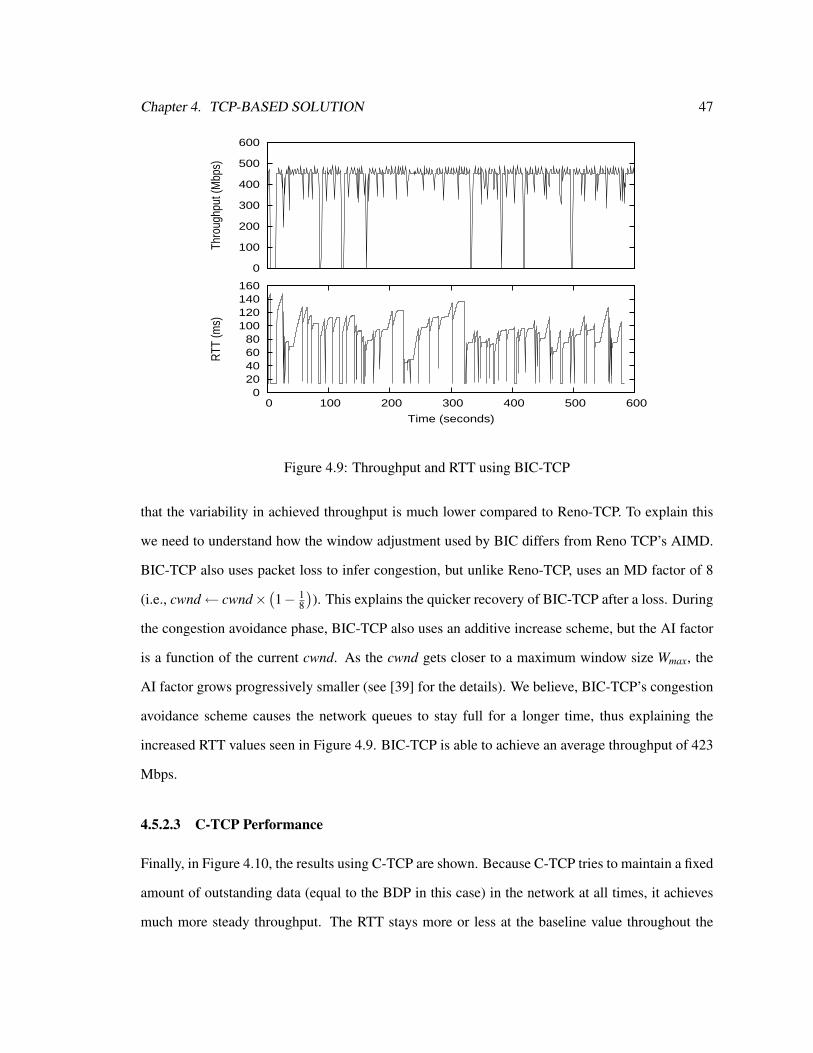
Chapter 4. TCP-BASED SOLUTION 47
0 20 40 60 80
100 120 140 160
0 100 200 300 400 500 600
RTT
(ms)
Time (seconds)
0
100
200
300
400
500
600
Thro
ughp
ut (M
bps)
Figure 4.9: Throughput and RTT using BIC-TCP
that the variability in achieved throughput is much lower compared to Reno-TCP. To explain this
we need to understand how the window adjustment used by BIC differs from Reno TCP’s AIMD.
BIC-TCP also uses packet loss to infer congestion, but unlike Reno-TCP, uses an MD factor of 8
(i.e., cwnd← cwnd×(1− 1
8
)). This explains the quicker recovery of BIC-TCP after a loss. During
the congestion avoidance phase, BIC-TCP also uses an additive increase scheme, but the AI factor
is a function of the current cwnd. As the cwnd gets closer to a maximum window size Wmax, the
AI factor grows progressively smaller (see [39] for the details). We believe, BIC-TCP’s congestion
avoidance scheme causes the network queues to stay full for a longer time, thus explaining the
increased RTT values seen in Figure 4.9. BIC-TCP is able to achieve an average throughput of 423
Mbps.
4.5.2.3 C-TCP Performance
Finally, in Figure 4.10, the results using C-TCP are shown. Because C-TCP tries to maintain a fixed
amount of outstanding data (equal to the BDP in this case) in the network at all times, it achieves
much more steady throughput. The RTT stays more or less at the baseline value throughout the

Chapter 4. TCP-BASED SOLUTION 48
0 20 40 60 80
100 120 140 160
0 100 200 300 400 500 600
RTT
(ms)
Time (seconds)
0
100
200
300
400
500
600
Thro
ughp
ut (M
bps)
Figure 4.10: Throughput and RTT using C-TCP
transfer. Thus, C-TCP does not stress the switch buffers. The average throughput achieved by C-
TCP was 458 Mbps. As pointed out in [5], keeping the network node buffers empty most of the
time gives lower end-to-end delay and, paradoxically, better throughput. This is because empty
queues serve to buffer bursts of packets, whereas if a queue was more likely to be full, then bursts
could cause packet losses and reduction in the cwnd by the sending host. Thus, the performance
improvement of C-TCP is expected to be more pronounced in the presence of interfering traffic.

Chapter 5
CONTROL-PLANE FUNCTIONS
In this chapter we consider issues associated with the control plane functions of a transport protocol
for dedicated circuits. The division into control and data plane functions is particularly clear in
a transport protocol for connection-oriented networks. Reservation of the network resources that
are subsequently used in the data plane transfer is a control plane function. The control plane
component of the transport protocol can be implemented independent of the data plane component,
i.e., the issues considered in this chapter apply equally to the UDP-based FRTP (Chapter 3) and
the TCP-based C-TCP (Chapter 4). For ease of exposition, we use “C-TCP” instead of “a transport
protocol for dedicated circuits” in the rest of this chapter.
The control plane functions of the transport protocol are divided into two parts. The first is the
selection of a circuit rate and is covered in Section 5.1. Once the circuit rate is selected, the required
amount of network resources need to be reserved. This part is covered in Section 5.2.
5.1 Selecting the Circuit Rate
Proper selection of the rate of the circuit to set up is important to achieve a balance between two
data transfer performance criteria. If a high-rate circuit is set up, and the end hosts are not capable
of maintaining data flow at that rate, circuit utilization will suffer. On the other hand, being over-
cautious and requesting a low-rate ciruit would lead to longer transfer delays than necessary.
The circuit rate should be set to the maximum data transfer rate that can be sustained by the
49

Chapter 5. CONTROL-PLANE FUNCTIONS 50
300
350
400
450
500
550
600
650
700
1 2 3 4 5 6 7 8 9 10
Thro
ughp
ut(M
bps)
Experiment run number
TCPC-TCP
Figure 5.1: Throughput variability of disk-to-disk transfers
end hosts involved. The problem thus boils down to finding out this sustainable rate. Variability
in the data sending and receiving rate at the end hosts can arise due to factors such as multitasking
(see Section 2.2.4) and disk access rate variability (see Section 2.2.3). This makes the selection of
the optimum circuit rate a difficult problem. To illustrate this, a set of disk-to-disk transfers were
carried out using a simple file transfer program that we implemented. The achieved throughput
values for transferring a 1.6 GB file between zelda3 and zelda4 (see Figure 4.5), over a 1 Gbps
circuit, are shown in Figure 5.1. The variability of the throughput evident in the ten runs using TCP
and C-TCP shows the difficulty in assigning a single number to the performance of disk-to-disk
transfers. A pragmatic approach to this problem is the following.
1. To the extent possible, we require users of C-TCP to reduce the sources of variability, e.g.,
by not running other processes while the data transfer is in progress. We believe this is a
reasonable requirement in the scientific computing domain.
2. Use an empirical method to estimate the average transfer rate that the end hosts can support.
The disk write rate is the limiting factor, hence a disk I/O benchmark program can be used to
estimate the average rate at which data can be written to disk on the receiving host.

Chapter 5. CONTROL-PLANE FUNCTIONS 51
15
20
25
30
35
40
400 500 600 700 800 900 1000 65
70
75
80
85
90
95
Tran
sfer
del
ay (s
econ
ds)
Circ
uit u
tiliz
atio
n (%
)
Circuit rate (Mbps)
Transfer delayUtilization
Figure 5.2: Trade-off between circuit utilization and delay
If circuit utilization is not an important requirement, a user might choose to run other processes
simultaneously with the data transfer. The circuit rate, in this scheme, is only an empirically esti-
mated average, and this makes flow control all the more important.
To test the utility of this approach, we used the method described next. First, we obtain a
value for the circuit rate for which disk-to-disk transfers get acceptable delay and circuit utilization.
Then we use a disk I/O benchmark to determine whether that circuit rate can be estimated using
the benchmark. In Figure 5.2, the transfer delay and circuit utilization (throughput/circuit rate) are
plotted against circuit rate for file transfers between zelda3 and zelda4. A 1.6 GB file was transferred
in each case and circuits with rates ranging from 400 Mbps to 1 Gbps were used. Average values
and standard deviation for five runs are shown.
There are a few points worth noting in this plot. First, the shape of the two graphs broadly
confirms our intuition that a better transfer delay can be achieved at the expense of circuit utilization
and vice versa. The transfer delay can be halved with a circuit rate of 1 Gbps as compared to a 400
Mbps circuit, but at the cost of a 20% reduction in the bandwidth utilization (70% compared to
85%). Second, for circuit rates greater than the end host supportable data transfer rate, the circuit

Chapter 5. CONTROL-PLANE FUNCTIONS 52
Disk Write Rate (Average ± Std. Dev.) MbpsRequest Size KB Normal I/O Synchronous I/O Direct I/O
8 1956 ± 45.0 892 ± 63.8 679 ± 4.716 2238 ± 32.0 919 ± 12.2 990 ± 5.932 2333 ± 40.3 954 ± 54.2 893 ± 41.664 2417 ± 41.7 926 ± 30.4 910 ± 79.3128 2456 ± 54.6 904 ± 55.8 955 ± 84.5
Table 5.1: xdd benchmark results on zelda4
Run # 1 2 3 4 5 6 7 8 9 10Normal I/O 2315 2349 2341 2320 2273 2427 2324 2341 2298 2336
Synchronous I/O 1023 924 901 1010 945 922 933 1055 905 926Direct I/O 886 935 933 922 855 928 930 817 867 862
Table 5.2: Disk write rate (Mbps) for individual runs using 32 KB request sizes
rate is no longer the bottleneck, therefore the transfer delay should remain more or less constant. In
the figure, the plot for transfer delay appears to flatten out for circuit rates greater than 700 Mbps.
Thus, from this figure, an optimum circuit rate value of 700 Mbps can be inferred.
Now we need to determine whether a disk I/O benchmark can be used to estimate this opti-
mum circuit rate before setting up the circuit. We use the xdd (version 6.3) disk I/O benchmark
program [32], to gather disk write rate estimates for three types of disk write operations— normal,
synchronous and direct I/O. Normal I/O makes full use of the page cache, synchronous I/O ensures
that data in the page cache and on the disk is synchronized and direct I/O bypasses the page cache
entirely. For a more detailed explanation of how disk writes are handled in the Linux kernel see
Appendix A or [4]. The xdd program was used to write 1 GB files using different request sizes.
The file size divided by the request size determines the number of write operations (calls to write()
system calls) performed by xdd. In Table 5.1 the average disk write rate and its standard deviation
on the zelda4 host, for ten runs, using five request sizes is shown. In Table 5.2, the disk write rates
for individual runs, using a 32 KB request size, are shown. The operating system, file system and
amount of RAM on zelda4 were Linux 2.6.11, ext3 and 2 GB, respectively.
These results show that the disk write rate estimated by the benchmark is higher than the circuit
rate that was inferred from Figure 5.2. This is true for all three kinds of disk I/O. The disk write

Chapter 5. CONTROL-PLANE FUNCTIONS 53
rate achieved using normal I/O, e.g., is more than three times the 700 Mbps number we were
expecting. This difference is explained by the fact that when data is being received over a circuit
and then written to disk, the network processing also plays a part. With the disk I/O benchmark
experiments only the disk write path is being tested and the interaction between the disk I/O and
network processing is ignored. Such interactions might include, for instance, contention for the
memory bus (see Section 2.2.1), or scheduling of the disk write and the network handling kernel
code paths. Also notice the large values for the standard deviation of the disk write rates. Direct
I/O gives a stable value for the achieved rate when request sizes of 8 KB and 16 KB are used, but
the variability in write rate increases dramatically for larger request sizes. For more results using
the xdd benchmark and possible explanations, see Appendix A. Thus, finding the optimal circuit
rate is not as straightforward as estimating the disk write rate on the receiver. First, the estimate for
the disk write rate has a large variability. Second, there are factors that cannot be accounted for by
a benchmark that estimates disk I/O performance.
5.2 Setting up the Circuit
Network resources need to be reserved before data transfer can begin. The actual circuit set-up
is handled by the RSVP-TE client implementation. The current implementation of the RSVP-TE
client [41], is in user space. It provides an API through a library as well as an application program
called bwrequestor (for bandwidth requestor) that can be called from the command-line to set up a
circuit. An application that wants to use a dedicated circuit would make API calls to the RSVP-TE
library. Occasionally, though, it may not be possible to modify an application to make such calls.
The bwrequestor can be used to set up a circuit in such cases. C-TCP interacts with the signaling
module differently in these two cases.
For applications that wish to use C-TCP over a dedicated circuit, and can be modified to do
so, an API is provided that closely matches TCP’s sockets API. The C-TCP API modifies only the
connect() and accept() calls from the TCP API. The C-TCP calls are actually wrappers around the
TCP calls. Thus, a system call syscall() is wrapped into the C-TCP specific syscallCTCP() that is

Chapter 5. CONTROL-PLANE FUNCTIONS 54
implemented like a regular user space function:
syscallCTCP() {
/* C-TCP specific operations */
...
syscall();
/* C-TCP specific operations */
...
}
There are two reasons for choosing this approach. The RSVP-TE signaling library that is used by
C-TCP is implemented in user space, and therefore calls to these functions have to originate from a
user space program. Second, applications must still be able to make calls to syscall() directly.
The C-TCP API provides four calls that differ from the TCP sockets API. The connect() call’s
functionality is provided by CTCP sender connect() and CTCP receiver connect(), and the ac-
cept() call’s functionality is provided by CTCP sender accept() and CTCP receiver accept(). The
names of the API calls indicate whether they are invoked by the data sender or receiver. In any data
transfer application using TCP, there will be a separation between the end that invokes connect() and
the one that invokes listen()/accept(). Because of the similarity between initiating a TCP connection
using connect() and setting up a circuit, C-TCP initiates circuit set up from the end that invokes the
C-TCP equivalent of connect(). The end initiating circuit set up needs to know the circuit rate, and
the circuit rate is determined by the receiving end host’s capability, hence it needs to know which
end is the receiver. One way to do this would be by imposing strict constraints on who (sender or
receiver) can invoke which call (connect or accept). For instance, only the data sender could be
allowed to invoke the connect() call. Instead, since the application knows whether it is the sender
or receiver, we take the approach of providing different calls for the sender and receiver, leaving it
to the application programmer to make the appropriate call. Within the wrapper calls, two kinds of
Chapter 5. CONTROL-PLANE FUNCTIONS 55
C-TCP specific operations are performed. The first is circuit set up using the RSVP-TE library and
the second is setting up the C-TCP parameters (see Section 4.4.2) using the Web100 API.
There may be some applications which cannot be modified to use the C-TCP API. To allow
such applications to use CHEETAH circuits, we use the following scheme. The bwrequestor is
used to set up a circuit. Because the C-TCP parameters useckt and ncap are actually fields in the
data structure associated with a TCP socket, they cannot be set until the TCP socket is created. We
have implemented a C-TCP Work Around Daemon (CTCP-WAD, the name is borrowed from a
similar daemon implemented in the Web100 project). The bwrequestor, after successfully setting
up a circuit, informs the CTCP-WAD about the circuit rate and the source and destination IP ad-
dresses of the circuit. The CTCP-WAD then periodically checks for TCP sockets which match this
source/destination IP address pair and when such a TCP socket is found, sets the C-TCP parameters
for that socket.

Chapter 6
CONCLUSIONS
In this chapter we summarize the key lessons learned from our efforts. A few ideas for future work
to advance the present work are also presented.
6.1 Conclusions
6.1.1 Transport Protocol Design for Dedicated Circuits
• The transport protocol can be split into control and data plane components. The control plane
functions are selecting the rate of the circuit to set up for a particular data transfer and setting
up the circuit.
• The data plane component of the transport protocol should be designed such that a data
transfer makes the best possible use of the reserved network resources. Ideally, this can be
achieved by matching the data transfer rate and the reserved circuit rate.
• In addition to the high utilization goal, the transport protocol should maximize the data trans-
fer rate in order to reduce the end-to-end delay.
• In practice, it is hard to match the data transfer rate and the reserved circuit rate exactly,
throughout the data transfer. Therefore, the protocol should try to avoid situations that cause
the data transfer rate to deviate from the circuit rate.
56

Chapter 6. CONCLUSIONS 57
• Flow control is required because of the lack of resource reservation on the end hosts.
6.1.2 Transport Protocol Implementation
• We implemented Fixed Rate Transport Protocol (FRTP), a user-space, UDP-based protocol,
by modifying SABUL. The advantage of a user-space implementation is ease of deployment.
The shortcomings of FRTP were the need for busy waiting to maintain a fixed data transfer
rate, and the lack of any form of flow control.
• The need for more support from the kernel, especially for flow control, led to the implementa-
tion of Circuit-TCP (C-TCP). C-TCP has been implemented by modifying the TCP/IP stack
in Linux. It maintains a fixed amount of outstanding data in the network and uses TCP’s self
clocking property to maintain a fixed data transfer rate that is closely matched to the reserved
circuit rate.
• Results of experiments on the CHEETAH testbed show that C-TCP is better suited for use
over dedicated circuits compared to TCP. Data transfer time is reduced because C-TCP dis-
ables slow start. In addition, because C-TCP maintains a fixed amount of outstanding data
in the network, buffers in the network nodes do not fill up. Thus, C-TCP obtains a steady
throughput in sustained data transfers.
• There exists a mismatch between the network, in which resources can be reserved, and the
end hosts’ operating system that do not support resource reservation. This makes it difficult
to select a circuit rate such that both circuit utilization and data transfer delay are optimized.
6.2 Future Work
The control plane problem of determining an optimal circuit rate has to be addressed. It is difficult to
model all the factors that play a part in determining the optimal rate. Therefore, a possible approach
could be to use the throughput values of past data transfers to get better and better estimates of the
sustainable data transfer rate. Estimates would need to be maintained for each sending-receiving

Chapter 6. CONCLUSIONS 58
end host pair, since end-host factors have the biggest impact on the sustainable data transfer rate
once a circuit is established.
Another direction for future work would be to study the impact of multitasking on C-TCP’s
ability to maintain a steady data transfer rate. It might be necessary to use an operating system
with real-time support. For instance, QNX is a commercial real-time operating system (RTOS).
Enhancements to the Linux kernel to provide real-time support, such as RTLinux and Real Time
Application Interface (RTAI) [31], are also available. The advantages of using an RTOS must be
justified against the costs of requiring a specialized operating system.

Appendix A
DISK WRITE RATE ESTIMATION
High utilization of a dedicated circuit for file transfers requires that the sending end keep the circuit
full and the receiving end be able to receive data at the circuit rate. Since file transfers involve
writing data to disk, a likely bottleneck is the rate at which data can be written to the disk, thus
making it crucial to estimate the disk write rate accurately. To do this we used xdd, a disk I/O
benchmark program. Results for the zelda4 host were presented in Section 5.1 and we pointed out
the problems involved in using such results to get a reliable estimate for the disk write rate. In this
appendix we present some background on how disk writes are handled in Linux. Benchmark results
for end hosts other than zelda4 are presented to show the effect of other factors.
A.1 How Linux Handles Disk Writes
The storage space on hard disks is divided into 512-byte sectors [4]. A sector is the minimum
amount of data that can be transferred from or to a disk. Device drivers in the operating system
kernel request data transfer in the size of blocks. Blocks consist of a set of adjacent bytes on the
disk, with the constraints that the block size (in bytes) should be a power of two, a multiple of the
sector size and smaller than the memory page size. Since, typically the page size is 4096 bytes,
block sizes of 1024 and 4096 bytes are commonly used. Each block on disk requires a buffer in
memory that is used by the kernel to store the block’s contents. There exists a buffer head data
structure, corresponding to each buffer, that contains information such as the memory address of
59

Appendix A. DISK WRITE RATE ESTIMATION 60
the buffer, the major and minor numbers of the device on which the block resides,1 the logical block
number etc.
Device drivers access blocks on the disk. Since physically moving the disk head to the area on
the disk where a block resides is expensive, the device driver tries to cluster together accesses to
adjacent blocks. To help with this clustering, device drivers are implemented with a high-level and
a low-level component. The high-level component forms requests for disk blocks. These requests
for individual blocks can be merged with existing requests for adjacent blocks. The kernel tries
to delay fulfilling disk access requests in order to allow more requests to be merged. Each device
driver has a list of request descriptors for requests that are pending. The low-level component of
a device driver goes through this list of requests and programs the disk controller to transfer each
block in each request.
Although every disk access has to go through the high-level device driver, and thus has to be
for disk blocks, it is much more convenient to access files in terms of virtual memory pages. Data
transfer for block devices can be classified into block I/O and page I/O. Block I/O operations transfer
a single block of data from disk that can be stored in a buffer in memory. Operations that access
filesystem metadata, such as inodes, use block I/O. Page I/O operations transfer a page’s worth of
blocks from the disk. These are invoked when accessing files (either regular files or device files like
/dev/hda). Although the data transferred in a page I/O operation is contiguous in the file of which it
is a part, the blocks comprising that page need not be contiguous on disk. For instance, with a page
size of 4096 bytes and a block size of 1024 bytes, a single page I/O operation might require that the
high-level device driver form four separate requests (recall that each request is for block(s) of data
that are contiguous on the disk).
To reduce disk accesses, and thus improve system performance, Linux uses disk caches. In [4],
a disk cache is defined as “a software mechanism that allows the system to keep in RAM some data
that is normally stored on disk, so that further accesses to that data can be satisfied quickly without
accessing the disk”. Two main disk caches are used in Linux, buffer cache and page cache. The
1The major and minor number of a device are used to differentiate between devices. The major number identifies thedevice type, e.g., IDE disk, and the minor number identifies a particular instance of that device, e.g., the third partitionon the second IDE disk.

Appendix A. DISK WRITE RATE ESTIMATION 61
buffer cache improves the performance of block I/O operations. The page cache consists of pages
that are involved in page I/O operations.
Consider a simplified version of how a write() system call to a file might proceed:
1. The arguments passed to the system call are filp, a pointer to the file to write to, buf, a pointer
to the user space memory from which to write, count, the number of bytes to write and ppos,
the offset in the file at which to write.
2. To quickly find out whether a particular portion of a file is in the page cache, a hash table is
maintained.
3. For each page of data to be written to the file on disk, the hash table for that file is consulted.
If the page is not in the page cache a new page is allocated.
4. If the page’s buffers do not already have corresponding buffer heads, they are allocated.
5. Data is copied from the user space buf to the page in the page cache.
6. The buffers which have been written to are marked as being dirty.
7. The responsibility of actually writing dirty buffers to the disk falls to a couple of kernel
threads— bdflush and kupdate. The bdflush thread is woken up when the proportion of page
buffers that are dirty exceeds a certain value. Each time a buffer is marked dirty the proportion
of dirty buffers is checked and if necessary bdflush is woken up. The kupdate thread helps
to ensure that a buffer that has been modified does not hang around in the disk cache for too
long. It is invoked periodically and flushes to disk all buffers that have been dirty for longer
than a threshold value.
These steps are applicable for a normal write to disk. Thus, if the amount of data written by
a process is small enough to fit entirely in the page cache without invoking bdflush or kupdate
immediately, then the writes can appear to be very fast. This is the common case scenario and
the page cache serves to improve its performance. A slightly different type of disk write is the
synchronous write. A process can ensure that all modified blocks are written to disk by using

Appendix A. DISK WRITE RATE ESTIMATION 62
system calls such as fsync() or sync() to synchronize the contents of the disk cache and the disk.
In addition, Linux also supports direct I/O that is useful for applications that do application-level
caching (e.g. database applications). For such applications, additional caching in the page cache
is not useful and might, in fact, slow things down because of the overhead of maintaining the page
cache data structures. Direct I/O can be requested by specifying a flag when a file is open()ed. For
direct I/O transfers, the kernel allocates special buffers that are visible from the user and kernel
space, so that no copying is necessary.
A.2 Benchmark Results
In this section we present the results of running the xdd disk I/O benchmark. After obtaining the
source code, compiling and installing xdd, it can be invoked from the command-line in the follow-
ing manner:
xdd.linuxsmp -op write -deletefile -targets 1 <filename> -reqsize
<request size> -mbytes <file size> -output <output file>
xdd is compiled for a Symmetric Multiprocessing (SMP) Linux machine.
-op specifies the operation to perform, read or write.
-deletefile instructs that the file written should be deleted once the transfer is over.
-targets 1 <filename> specifies the number and name(s) of the file(s) to be written.
-reqsize <reqsize> is the size of each I/O operation in KB.
-mbytes <file size> specifies the total size of the file to be written (MB)
-output <output file> specifies that xdd’s output statistics should be written to a file.
Four machines were used for the tests, in addition to zelda4, results for which were presented in
Section 5.1. The names and relevant configuration details for the four machines are shown in Ta-
ble A.1. Two different kernel versions were used on zelda3 to see the effect of the kernel on disk
write performance.
The average disk write rate and standard deviation of ten runs (in Mbps), for the five configura-
tions are shown in Table A.2. We can make the following observations from these results:

Appendix A. DISK WRITE RATE ESTIMATION 63
Host name OS/kernel File system RAM (GB)zelda1 Linux/2.4.21 ext3 2zelda2 Linux/2.4.21 ext3 2zelda3 Linux/2.4.21 ext3 2zelda3 Linux/2.6.11 ext3 2mvstu6 Linux/2.4.21 ext3 1
Table A.1: End host configurations
Request size (KB) Normal I/O Synchronous I/O Direct I/Ozelda1
8 1048 ± 85.7 794 ± 34.9 624 ± 2.516 1034 ± 33.9 787 ± 58.7 882 ± 4.932 1125 ± 82.0 788 ± 54.3 817 ± 49.164 1079 ± 64.6 782 ± 27.7 884 ± 14.4
128 1158 ± 92.5 800 ± 58.8 879 ± 86.9zelda2
8 979 ± 57.3 759 ± 42.1 623 ± 1.616 1041 ± 41.5 759 ± 51.8 880 ± 5.532 1109 ± 77.9 745 ± 22.7 805 ± 14.364 1085 ± 76.4 747 ± 24.4 862 ± 42.8
128 1121 ± 94.5 767 ± 15.1 846 ± 71.9zelda3 (2.4.21)
8 1115 ± 64.4 875 ± 69.0 626 ± 2.616 1208 ± 46.0 925 ± 60.5 888 ± 3.432 1233 ± 57.1 911 ± 44.4 984 ± 86.564 1241 ± 50.3 918 ± 56.3 972 ± 91.0
128 1239 ± 87.7 893 ± 50.0 987 ± 17.9zelda3 (2.6.11)
8 2062 ± 186.4 1000 ± 68.3 670 ± 11.916 2341 ± 18.6 988 ± 90.5 965 ± 23.832 2397 ± 46.6 956 ± 86.5 999 ± 89.464 2451 ± 34.7 995 ± 77.6 978 ± 45.9
128 2508 ± 51.8 984 ± 89.2 970 ± 98.5mvstu6
8 815 ± 89.6 614 ± 35.2 633 ± 2.216 858 ± 76.4 649 ± 24.6 895 ± 7.932 880 ± 117.4 637 ± 38.1 1112 ± 74.564 883 ± 53.3 656 ± 36.8 1054 ± 83.8
128 884 ± 94.8 647 ± 41.1 1018 ± 11.3
Table A.2: Disk write rate results using xdd

Appendix A. DISK WRITE RATE ESTIMATION 64
• Disk write rate achieved using normal I/O is higher compared to that achieved by synchronous
I/O. This is because a synchronous I/O write has the extra overhead of writing all dirty buffers
to disk.
• Direct I/O transfers seem to be the most affected by the request size. The general trend is that
the rate achieved using direct I/O increases as the request size increases from 8 to 32 KB, and
then either levels off or decreases slightly for request sizes of 64 and 128 KB. When using
direct I/O, data is written to the disk in request size chunks. As the request size increases,
each disk access transfers a larger amount of data. The dip in disk write rate for request sizes
above 32 KB is probably because for larger requests the likelihood of all blocks in the request
being close together reduces. Thus, the disk head requires more seek time to complete the
transfer.
• Next, consider the standard deviation values. The standard deviations are high for most
combinations of disk I/O type and request size, usually greater than 40 Mbps. The exceptions
are the direct I/O transfers using small request sizes.
• For direct I/O transfers, the variability in achieved rate increases as the request size increases.
For request sizes of 8 and 16 KB, the standard deviation for direct I/O transfers is often
smaller than 5 Mbps. But for request sizes larger than 16 KB the standard deviation increases
dramatically. The increase in seeks for larger request sizes also explains the increased vari-
ability of direct I/O, since the seek time depends on the position of the data on the disk.
• To see which type of I/O transfer is most affected by the request size, we can calculate the
standard deviation of the average disk write rates obtained using different request sizes. For
instance, the standard deviation of the average rates for zelda1 are 52, 7 and 111 Mbps for
normal, synchronous and direct I/O, respectively. In general, synchronous I/O appears to be
the least affected by request size value and direct I/O the most affected.
• Comparison of results for different kernel versions on zelda3 shows that normal I/O perfor-
mance improves almost two-fold, for all request sizes, on the 2.6.11 kernel. The disk schedul-

Appendix A. DISK WRITE RATE ESTIMATION 65
ing algorithm, which decides the order in which requests are sent to the disk controller, has
been improved in the new kernel. This is most likely the reason for the improvement in
performance of the normal I/O transfers.
• There is a slight improvement in the performance of synchronized I/O, but no noticeable
change in direct I/O performance when using the newer kernel. Synchronized and, especially,
direct I/O performance is dependent more on the disk capability itself rather than the kernel
disk scheduling algorithm.

Bibliography
[1] ALLMAN, M., PAXSON, V., AND STEVENS, W. TCP Congestion Control. RFC 2581 (Apr.
1999).
[2] ANDERSON, D. P., COBB, J., KORPELA, E., LEBOFSKY, M., AND WERTHIMER, D.
SETI@home An Experiment in Public-Resource Computing. Communications of the ACM
(Nov. 2002).
[3] BERTSEKAS, D., AND GALLAGER, R. Data Networks (2nd ed.). Prentice-Hall, Inc., Upper
Saddle River, NJ, USA, 1992.
[4] BOVET, D. P., AND CESATI, M. Understanding the Linux Kernel, 2nd Edition. O’Reilly
Media, Inc., 2002.
[5] BRADEN, B., CLARK, D., CROWCROFT, J., DAVIE, B., DEERING, S., ESTRIN, D., FLOYD,
S., JACOBSON, V., MINSHALL, G., PARTRIDGE, C., PETERSON, L., RAMAKRISHNAN, K.,
SHENKER, S., WROCLAWSKI, J., AND ZHANG, L. Recommendations on Queue Manage-
ment and Congestion Avoidance in the Internet. RFC 2309 (Apr. 1998).
[6] CHASE, J. S., GALLATIN, A. J., AND YOCUM, K. G. End-System Optimizations for High-
Speed TCP. IEEE Communications Magazine (Apr. 2001).
[7] CHU, H. K. J. Zero-Copy TCP in Solaris. Proc. USENIX Annual Technical Conference, San
Diego, CA (Jan. 1996).
[8] CLARK, D. D. Window and Acknowledgement Strategy in TCP. RFC 813 (July 1982).
66

Bibliography 67
[9] CLARK, D. D., JACOBSON, V., ROMKEY, J., AND SALWEN, H. An Analysis of TCP Pro-
cessing Overhead. IEEE Communications Magazine (June 1989).
[10] CLARK, D. D., LAMBERT, M. L., AND ZHANG, L. NETBLT: A Bulk Data Transfer Proto-
col. RFC 998 (Mar. 1987).
[11] CSMA/CD Access Method. IEEE 802.3 standard, section 2, appendix 31B.
[12] DRAGON Dynamic Resource Allocation via GMPLS Optical Networks.
http://dragon.east.isi.edu.
[13] FALL, K., AND FLOYD, S. Simulation-based Comparisons of Tahoe, Reno, and SACK TCP.
ACM Computer Communication Review (July 1996).
[14] FLOYD, S. HighSpeed TCP for Large Congestion Windows. RFC 3649 (Dec. 2003).
[15] FLOYD, S., AND JACOBSON, V. Random Early Detection Gateways for Congestion Avoid-
ance. IEEE/ACM Transactions on Networking (Aug. 1993).
[16] FLOYD, S., MAHDAVI, J., MATHIS, M., AND PODOLSKY, M. An Extension to the Selective
Acknowledgement (SACK) Option for TCP. RFC 2883 (July 2000).
[17] FOONG, A. P., HUFF, T. R., HUM, H. H., PATWARDHAN, J. P., AND REGNIER, G. J. TCP
Performance Re-Visited. Proc. International Symposium on Performance Analysis of Systems
and Software, Austin, TX (Mar. 2003).
[18] GU, Y., AND GROSSMAN, R. L. SABUL: A Transport Protocol for Grid Computing. Journal
of Grid Computing (Dec. 2003).
[19] GU, Y., AND GROSSMAN, R. L. UDT: An Application Level Transport Protocol for Grid
Computing. 2nd International Workshop on Protocols for Long-Distance Networks PFLDNet
(Feb. 2004).
[20] HE, E., LEIGH, J., YU, O., AND DEFANTI, T. A. Reliable Blast UDP: Predictable High
Performance Bulk Data Transfer. Proc. IEEE Cluster Computing (Sept. 2003).

Bibliography 68
[21] JACOBSON, V. Congestion Avoidance and Control. ACM Computer Communication Review
(Aug. 1988).
[22] JACOBSON, V., BRADEN, R., AND BORMAN, D. TCP Extensions for High Performance.
RFC 1323 (May 1992).
[23] JIN, C., WEI, D. X., AND LOW, S. H. FAST TCP: Motivation, Architecture, Algorithms,
Performance. IEEE Infocom (Mar. 2004).
[24] KATABI, D., HANDLEY, M., AND ROHRS, C. Congestion Control for High Bandwidth-
Delay Product Networks. ACM Sigcomm (Aug. 2002).
[25] KELLY, T. Scalable TCP: Improving Performance in Highspeed Wide Area Networks. ACM
SIGCOMM Computer Communication Review (Apr. 2003).
[26] MATHIS, M., HEFFNER, J., AND REDDY, R. Web100: Extended TCP Instrumentation. ACM
Communications Review (July 2003).
[27] MATHIS, M., MAHDAVI, J., FLOYD, S., AND ROMANOW, A. TCP Selective Acknowledge-
ment Options. RFC 2018 (Apr. 1996).
[28] PIETIKAINEN, P. Hardware-assisted Networking Using Scheduled Transfer Protocol on
Linux. Diploma thesis, Dept. of Electrical Engineering, University of Oulu, Oulu, Finland
(Sept. 2001).
[29] POSTEL, J. Transmission Control Protocol. RFC 793 (Sept. 1981).
[30] RAMAKRISHNAN, K., FLOYD, S., AND BLACK, D. The Addition of Explicit Congestion
Notification (ECN) to IP. RFC 3168 (Sept. 2001).
[31] RTAI Real Time Application Interface. http://www.rtai.org.
[32] RUWART, T. M. Xdd User’s Guide. http://www.ioperformance.com/xddversions/xdd6.3.pdf,
Jan. 2005.

Bibliography 69
[33] STEENKISTE, P. A Systematic Approach to Host Interface Design for High-Speed Networks.
IEEE Computer (Mar. 1994).
[34] STEVENS, W. R. TCP/IP Illustrated, Volume 1: The Protocols. Addison-Wesley Professional,
Boston, MA, USA, 1993.
[35] TIRUMALA, A., QIN, F., DUGAN, J., FERGUSON, J., AND GIBBS, K. Iperf Version 1.7.0.
http://dast.nlanr.net/Projects/Iperf/, Mar. 2003.
[36] DOE UltraScience Net : Experimental Ultra-Scale Network Testbed for Large-Scale Science.
http://www.csm.ornl.gov/ultranet/.
[37] VEERARAGHAVAN, M., ZHENG, X., LEE, H., GARDNER, M., AND FENG, W. CHEETAH:
Circuit-switched High-speed End-to-End Transport Architecture. Proc. of Opticomm (Oct.
2003).
[38] WU, Q., AND RAO, N. S. V. Protocol for High-Speed Data Transfer Over Dedicated Chan-
nels. 3rd International Workshop on Protocols for Long-Distance Networks PFLDNet (Feb.
2005).
[39] XU, L., HARFOUSH, K., AND RHEE, I. Binary Increase Congestion Control for Fast Long-
Distance Networks. IEEE Infocom (Mar. 2004).
[40] ZHENG, X., MUDAMBI, A. P., AND VEERARAGHAVAN, M. FRTP:Fixed Rate Transport
Protocol- A Modified Version of SABUL for End-to-end Circuits. First IEEE Workshop on
Provisioning And Transport for Hybrid Networks PATHNets, San Jose, CA (Sept. 2004).
[41] ZHU, X., ZHENG, X., VEERARAGHAVAN, M., LI, Z., SONG, Q., HABIB, I., AND RAO,
N. S. V. Implementation of a GMPLS-based Network with End Host Initiated Signaling.
submitted to IEEE ICC (June 2006).


![An end-to-end channel allocation scheme for a wireless … · An end-to-end channel allocation scheme for a wireless ... Internet protocol over WMNs [11]. This study proposes an end-to-end](https://static.fdocuments.net/doc/165x107/5b5a10eb7f8b9a6c4f8e2359/an-end-to-end-channel-allocation-scheme-for-a-wireless-an-end-to-end-channel.jpg)


![[MS-ASDSP]: Access Services Database Stored …...1.5 Prerequisites/Preconditions This protocol operates between a protocol client and a protocol server on which the back-end](https://static.fdocuments.net/doc/165x107/5edffb54ad6a402d666b4058/ms-asdsp-access-services-database-stored-15-prerequisitespreconditions.jpg)