A Transport Process Approach toUnderstanding Monte Carlo TransportMethods

Thomas E. Booth

Los Alamos National Laboratory, Diagnostic Applications Group X-5,Mail Stop F663, Los Alamos, New Mexico, 87545 USA email teb@lanl.gov

Abstract. Monte Carlo particle transport is usually introduced primarily as amethod to solve linear integral equations such as the Boltzmann transport equation.This focus on solving integral transport equations gives rise to a number of commonmisconceptions about MCNP transport methods among many MCNP users.

A transport process approach that is often useful in understanding the variancereduction in MCNP focuses directly on the Monte Carlo sampling process itself.

1 Introduction

Many MCNP users understand Monte Carlo transport theory via linear in-tegral equations. This is quite understandable as standard books in the fieldusually emphasize the connection of Monte Carlo transport and the trans-port equation. This connection has proven very useful both for teaching aboutMonte Carlo and for developing and analyzing many variance reduction meth-ods. The success of the books also indicates that the readers have found thetransport equation approach to understanding Monte Carlo transport useful.Indeed, the fact that so many Monte Carlo books emphasize the transportequation indicates that the experts writing the books have found the trans-port equation a very useful perspective both in practice as well as in teaching.

Monte Carlo books are written for many purposes, for example, as coursetextbooks and to illustrate the main ideas in the field. To my knowledge, noneof the standard Monte Carlo transport theory books were written with theintent of covering MCNP variance reduction methods; the books are intendedfor a more general readership. It would therefore be unreasonable to expect tounderstand MCNP variance reduction based solely on standard Monte Carlotransport theory books. For example, there is no standard book that justifiesthe unbiasedness of arbitrary combinations of MCNP’s variance reductiontechniques.

This report has four main purposes

1. to explain the transport process approach to variance reduction methodsin MCNP

2. to educate MCNP users about the sometimes significant differences be-tween the theory that they typically read in the Monte Carlo books andwhat MCNP actually does

3. to caution MCNP users about interpreting Monte Carlo transport usingthe wrong transport equation

4. to illustrate some aspects of statistical weight that are often not consid-ered by MCNP users

The “transport process” approach focuses on the Monte Carlo transportprocess itself to try and determine what the major sources of variance arein the simulation and what to do about these sources. The transport processapproach is a general approach that is useful for all MCNP calculations. Thetransport process approach to variance reduction can be especially usefulwhen the user has no integral transport equation results available, as is oftenthe case for typical MCNP calculations.

Before proceeding with the transport process approach, note that under-standing the transport process is not a substitute for understanding integraltransport equations. Integral transport equations can sometimes produce re-sults that would be very difficult, if not impossible, to produce by focusingsolely on a transport process approach.

By examining the transport process as one sets up the variance reductionin MCNP, one often finds that particles contributing most to the varianceare somewhat special. They may, for instance, tend to

1. have fewer collisions than typical particles2. have large distances between collisions in one direction and short dis-

tances between collisions in another direction3. have different energies or directions than typical particles4. have very different weights in a region than typical particles

Once the MCNP user has analyzed what is special about the particles con-tributing most to the variance, he may be able to use variance reductiontechniques to increase the sampling of these special particles.

MCNP users sometimes try simply tinkering with the values of MCNPvariance reduction parameters without having examined what types of parti-cles are contributing most to the variance. Unless the user’s intuition and/orluck is very good, this approach is usually far from optimal. A few observa-tions about MCNP users and variance reduction in the next two paragraphsmay help illustrate the usefulness of adding a transport process approach totheir variance reduction considerations.

An MCNP user’s intuition is often based on some (sometimes good, some-times perhaps very rough) notion of the importance function. This is usefulknowledge about a particle’s expected score. One can sometimes glean use-ful information about typical scoring particles. On the other hand, in manyhigh variance situations the typical scoring particle may have little influenceon the variance because the variance may be dominated by atypical scoringparticles. It is often difficult to have an idea what causes the variance in acalculation by knowing what causes the mean. Stated very simply, when at-tempting variance reduction it pays to focus on a measure of the variance

rather than the importance, which is a measure of the mean. MCNP usersshould understand that the importance function deals with the mean score,not the variance.

My experience dealing with MCNP users is that they tend to focus theirefforts on getting lots of low weight particles to the detector region. Theclearest example is that most (novice) MCNP users intuitively view a dxtransphere as “a magnet for pulling low weight particles” to the sphere ratherthan as “a shield against high weight particles” trying to cross the sphere.Dxtran can serve both purposes, of course. Using dxtran as a magnet tendsto focus on bringing lots of typical low weight particles into a detector region.The contribution to the mean is then dominated by these low weight particles.On the other hand, the contribution to the variance is then often dominatedby a few high weight particles. Roughly speaking, viewing dxtran as a magnetis consistent with producing typical scoring particles whereas viewing dxtranas a shield is consistent with precluding the high weight particles that mightotherwise dominate the variance.

2 Comments on “Analog” Monte Carlo and theTransport Process

Probably most Monte Carlo transport practitioners understand and use theterm “analog Monte Carlo” in mostly the same way. That is, convenient prob-ability densities are abstracted from the physical transport process. Theseconvenient probability densities are then embedded in a transport code. Forexample, the neutron distance to collision is sampled conveniently from anexponential distribution without modeling the detailed interactions betweenthe neutron and each nuclide along its path.

For this report, the term “analog” describes a direct sampling of these ab-stracted probability densities. For the most part, people have abstracted verysimilar probability densities from the physical transport process. Nonetheless,it is probably worthwhile to note that an analog sampling in the context ofthis report refers to the particular probability densities that MCNP has ab-stracted from the physical transport process. Roughly speaking, an analogMonte Carlo sampling of a neutron transport problem in MCNP is what onegets when no variance reduction techniques are used.

The term “transport process” is also used in the context of MCNP’sabstraction of the physical transport process. An analog transport process isan analog simulation of the abstracted physical transport process. Similarly,a nonanalog transport process is a nonanalog simulation of the abstractedphysical transport process.

A transport process approach focuses on the details of the simulation totry and determine what the major sources of variance are in the simulationand what to do about these sources.

3 Comments on Mathematics

Although many people have commented that particle transport can be sim-ulated without reference to the transport equation, this does not mean thatmathematical equations are irrelevant to MCNP. Except for the simple caseof an analog simulation, mathematical equations are necessary in both thetransport equation approach and the transport process approach. When thesimulation deviates from an analog simulation, both approaches require math-ematical equations to show that the mean estimates are preserved.

4 Caution on “The” Transport Equation

In most cases, Monte Carlo codes allow estimation of quantities for which thetransport equations displayed in the literature do not apply. In particular, thetypical transport equations totally ignore the correlation between particles.Thus any estimate, such as the pulse height tally in MCNP, that depends onthe correlation between particles is typically ignored. Transport equations, ofcourse, can be written to include correlation between particles, but authorstypically choose not to display such equations. If an MCNP user wishes to usetransport equations to analyze and/or improve his Monte Carlo calculation,it is important to understand what transport equations are relevant to thecalculation. This last statement seems obvious, but people have sometimestalked about the pulse height tally in MCNP in the same breath as a transportequation that ignores the correlation between particles.

5 Variance Reduction for Difficult Problems

For many problems, Monte Carlo estimates can often be obtained to suffi-cient precision using little or no variance reduction. This report assumes thatthe transport problems under consideration are sufficiently difficult that theMonte Carlo user needs to get close to the most efficient calculation that canbe run with MCNP.

Note that one of the answers to a transport problem is the calculationalvariance; it is not governed by the transport equation. At this point, twotypical approaches are:

1. One uses one’s intuition (often guided by some knowledge of the im-portance function) to set up the variance reduction and assumes thatwhatever variance results will be close to optimum.

2. One derives equations for the variance (or sometimes the product of thevariance of the mean and the computer time cost = σ2

mT ) as a functionof some parameters. One then solves these equations (sometimes usingresults from short Monte Carlo runs) for the optimum parameters. See[5, chapter 7] for a number of examples.

The first approach often works well if one’s intuition is good and onecan arrange the sampling so that there is a relatively small spread in historyscores. That is, each history contributes roughly the mean score. In this case,both the bulk of the mean and the bulk of the variance are produced bythe same particles. That is, focusing on particles that contribute most to thesecond moment is similar to focusing on particles that contribute most tothe mean. Indeed, in the limiting case of a zero variance solution all particlescontribute exactly the mean score and there is no reason to consider thesecond moment at all.

The other side of the coin is that the available variance reduction tech-niques may not allow one to arrange the sampling so that there is a relativelysmall spread in history scores. Alternatively, the variance reduction tech-niques may allow one to arrange the sampling so that there is a relativelysmall spread in history scores, but the user may not a priori be able to guesshow. In these cases, the set of particles contributing most of the variance maybe very different from the set of particles contributing most of the mean. Forinstance, the set of typical particles that contribute 99 percent of the meanmight only contribute 1 percent of the variance. In this case, focusing effortson typical particles that score will not work very well because the typical par-ticles are very different from the particles contributing most to the variance.One would do better to base the variance reduction on the second momentequation rather than the importance.

Concerning the second approach, if one views the mean transport (firstmoment) as resulting from a solution of the transport equation, then it isnatural (and often useful) to derive a similar equation for the second mo-ment (e.g. see[5, chapter 5]). Unlike the transport equation, note that anequation for the second moment depends on what variance reduction meth-ods one uses. (At this point, it is almost universal practice to consider onlytransport processes that are independent of particle weight.) The optimumsecond moment is, of course, optimal only for the particular set of variancereduction methods considered. This second approach works well when thevariance reduction methods considered in the optimization are a good matchto sources of variance in the problem. For example, particle penetration ofsimple slabs often can be done reasonably well by optimizing “cell impor-tances” (the geometry splitting and Russian roulette technique in MCNP.)If there is a streaming path, such as a duct running through the slab, theneven optimum cell importances may not sufficiently reduce the variance tomake the problem tractable with reasonable amounts of computing time.

6 Two Theoretical Results for the Transport ProcessApproach

Most of the theoretical results presented in standard Monte Carlo texts applyto only small subsets of the MCNP variance reduction methods. There arethree main reasons why these results are inadequate for MCNP purposes.

1. The results are typically restricted to weight independent simulations inwhich the random walk sampling does not depend on the particle weight.

2. The results do not consider arbitrary combinations of variance reductionmethods, typically not even arbitrary combinations of weight independentmethods.

3. MCNP is an open code so that users can add their own variance reductionmethods if they wish.

Consider the combination of variance reduction techniques. Until about1990, the following was true[6]:

“Nonanalog Monte Carlo techniques are essential to many calcula-tions, and historically they have been developed one at a time asneeded. Each new nonanalog technique usually, at best, has beenproven to preserve the expected tallies (i.e., be unbiased) when usedby itself. The techniques have not been proven to be unbiased inarbitrary combinations.”

Reference [5] has one of the better treatments, proving via integral equationsthat the combination of splitting and biased kernels is unbiased. If, in addi-tion to splitting and biased kernels, another variance reduction technique isadded, then one has to rewrite the integral equations to include the new tech-nique and prove unbiasedness via the new integral equation. MCNP relies onthe fact that any combination of Monte Carlo techniques is unbiased if thetechniques are individually unbiased. In statistical parlance, any combinationof fair games is also a fair game. This is a general statistical result for anylinear Monte Carlo process in any field, not just the transport field[6].

Before leaving the subject of “combinations of fair games,” note that[6] was controversial when it was reviewed. One reviewer initially sent ina two line review saying that the result was “well known” and “trivial” aswell. When challenged to produce either a reference or supply a proof, thereviewer did neither. The paper was then accepted, although the revieweremphasized that he still considered the result “trivial”. Since publication,several knowledgeable Monte Carlo practitioners also have asserted that thefair games result can be proven easily. There is little reason to doubt thatthe proof in [6] is not the simplest possible proof. The MCNP documentationcould be improved by inclusion of, or at least reference to, a simple proofthat any combination of fair games is also a fair game. Please send anysuch proposed proofs (for the MCNP manual) to mcnp-forum@lanl.gov forassessment and comment by the MCNP community.

A second example of a general statistical result is the subject of zerovariance methods. Zero variance solutions usually are derived solely in thecontext of importance biasing in the solution of an integral equation. To makematters even more specific, zero variance solutions are often derived only forlast event estimators, instead of for general estimators. From much of theliterature, one might erroneously conclude that there is only one way to get

a zero variance solution. Most discussions in the literature ignore the factthat zero variance solutions can be obtained[3] using any other collection ofvariance reduction techniques in addition to importance biasing. The generalrule to obtain a zero variance solution is to weight the sampling probabilityfor each outcome to be proportional to the outcome’s usual probability timesthe expected score generated if that outcome occurs. (Reference[3] showsone simple way to accomplish this sampling by expected score weighting thesampling of random numbers.) The usual derivation via importance samplingan integral equation is just one simple example of the general rule. Again notethat this is a general statistical result for any linear Monte Carlo process inany field, not just the transport field.

7 A Caution on Optimal Sampling Claims for MCNP

A common mistake in verbal and written communications is to mix weightindependent results from the literature together with the weight dependenttransport processes in MCNP. Unless carefully qualified, such communica-tions are often either false, misleading, or both.

A typical claim is that sampling from an importance weighted probabilitydensity minimizes the variance in an MCNP calculation. That is, if f(P ) isthe true probability density for sampling the next phase space point and I(P )is the importance function, then a typical claim is that sampling from thebiased probability density

b(P ) =f(P )I(P )

∫f(P )I(P ) dP

minimizes the variance. Sometimes the claim is put forth as so obvious thatno justification for the claim is supplied. Sometimes the claim is justifiedby reference to an importance sampling technique, despite the fact that thereferenced importance sampling result was not derived in the presence of aweight dependent simulation.

Whenever one is using weight dependent MCNP techniques, one shouldbe wary of assertions based on weight independent derivations in the litera-ture. It is perhaps worthwhile to note that MCNP plays a number of weightdependent games by default. For example, if one wants an analog MCNP cal-culation then in addition to not explicitly requesting any variance reduction,one must explicitly turn off the default weight cutoff game. As a result, almostall MCNP calculations are weight dependent simulations and the standardresults from weight independent theories do not apply.

8 Comments on Transport Equations and VarianceReduction in MCNP

Given the emphasis that standard books give to integral transport equationswhen discussing variance reduction, it is perhaps worthwhile to summarize

the current state of affairs with regard to transport equations and MCNP.Three reasonable questions are:

1. Why does MCNP use weight dependent simulations?2. Why not analyze weight dependent MCNP simulations using integral

transport equations?3. Why analyze MCNP simulations using a transport process approach?

Weight independent simulations can be viewed as a special case of moregeneral weight dependent simulations in the same sense that f(x) = constantcan be viewed as a special type of function of x. Philosophically, it is not verysurprising that selecting from a broader class of variance reduction techniquesmight allow for better variance reduction, but the primary reason that weightdependent simulations are allowed in MCNP is that they have proven usefulin practice.

The answers to the second and third questions are a bit more difficultand the answers may change eventually depending on future developments inMonte Carlo transport theory. At the present time, here are some thoughtson why transport equation analysis might be useful for weight dependentsimulations and why a transport process analysis is currently useful for weightdependent simulations.

1. Transport equations for the variance, usually via second moment equa-tions, (e.g. [5, chapter 5]) are currently almost exclusively for weight inde-pendent simulations. There is apparently no essential difficulty derivingweight dependent transport equations for the variance. To date though,I know of no use ever made of such an equation. This may change in thefuture.

2. Note that integral transport equations often are concise and easily in-terpretable. The fact that integral transport equations are an averageover the transport process can be a big advantage if one can effectivelyuse a transport equation that averages over unimportant aspects of thetransport process while preserving the important aspects of the transportprocess.

3. Although the transport process details have to have at least as muchinformation as any integral equation average over the process, there isalways the danger that useful general insights get lost in the details.

4. Inasmuch as nobody has figured out yet how to effectively use integralequations for the second moment in typical weight dependent MCNPcalculations, it is difficult to assess what general insights (from the secondmoment equation) currently might be hidden in the transport processdetails.

5. A transport process approach to variance reduction in MCNP is some-what of a necessity given the comments in items 1 and 4.

6. Many different fields have similar types of simulation processes so thattechniques used for processes in one field are often useful techniques inother fields as well.

7. By examining in detail the particles having the largest contributions tothe variance, it is often quite easy to identify the major source of variancestill left in an MCNP problem.

9 Markov and Nonmarkov Processes and RandomWalks

In MCNP’s analog simulation of nature, the next step of a particle’s randomwalk depends only on its current phase space location P . That is, MCNP’sanalog process is a Markov process.

Nonanalog simulations of particle transport depart, in one way or another,from the analog process. Nonanalog methods are also known as variancereduction methods because the intent of using nonanalog methods is to reducethe variance in the estimated mean for a given computer time. Note thatnonanalog simulations need not be Markov processes.

The following sections will comment on four categories of random pro-cesses

1. Processes depending only on the current phase space location P .2. Processes depending on all the random walk’s past physical events, e.g.

P0, P1, P2, · · · , Pn.3. Processes depending both on the current phase space location P and the

current statistical weight w.4. Processes not included in the previous items.

10 Natural Markov Processes

When the sampling of the particle depends only on the current phase spaceposition P , as it does in an analog MCNP modeling of nature, the samplingwill be said to be a natural Markov process. Many of the common variancereduction techniques are naturally Markovian. For example:

1. Biasing the transport kernels.– exponential transform in MCNP (path length stretching)

2. Splitting techniques– geometry splitting and Russian roulette in MCNP– survival biasing in MCNP (split into absorbed and surviving parts)– forced collisions in MCNP (split into collided and uncollided parts)

(MCNP is not remarkable in having variance reduction techniques that arenaturally Markovian; nor are the above techniques necessarily unique toMCNP. Transport codes sometimes differ both in their terminology andin their implementations of techniques having similar names. Specifying anMCNP technique makes the definition unambiguous, so that the categoriza-tion above is possible.)

There are variance reduction methods that are natural Markov processesand there are variance reduction methods that are not natural Markov pro-cesses. In general, the natural Markov processes are easier to study math-ematically because the next step of a particle’s random walk depends onlyon its current phase space location. Because of this simplicity, the pages ofMonte Carlo transport theory literature devoted to natural Markov processesfar exceeds the pages devoted to other Monte Carlo processes.

11 A Simple Nonmarkov Process

Reference[2, page 87] discusses a simple nonmarkov process in which thetransport probabilities can depend on the current and all the previous phasespace points, P1, P2, · · · , Pn. On the same page, the book says “ ... for thosefamiliar with the term, we shall be dealing almost exclusively with Markovprocesses. Nonetheless, it seems worth pointing out that nonmarkov pro-cesses may be treated as well.” Indeed, the remainder of the book almostexclusively considers transport problems with analog and nonanalog MonteCarlo simulations that depend solely on the current phase space point.

From an MCNP perspective, the reason that [2] usually does not apply toMCNP calculations is not so much that the previous phase space points arenot considered, it is that the particle weight is not included in the currentstate of the particle. That is, the nonanalog Monte Carlo simulations in [2]only seem to use weight independent random walks.

Returning to the book’s[2] notion of a nonmarkov random walk, note thatincluding the previous phase space points is occasionally useful. For example,MCNP allows consideration of events before the current phase space point Pvia the cell and surface flagging options. If a cell is flagged, then the tally ispartitioned into the part of the tally due to particles that have entered theflagged cell and the part of the tally due to particles that have not enteredthe flagged cell. The surface flag operates similarly. Although the productionversion of MCNP does not use different transport methods depending on theflag, it is easy and occasionally useful to modify MCNP to do so.

12 Weight Dependent Markov Processes

Many, probably most, of the common variance reduction techniques that arenot natural Markov processes depend only on the the current phase spacepoint P and the current weight w. Those processes whose transport dependsonly on (P,w) will herein be called weight dependent Markov processes todistinguish them from natural Markov processes.

Common weight dependent Markov processes in MCNP involve:

1. weight windows2. weight cutoff (associated with the geometry splitting/roulette)

3. weight dependent roulette games associated with point detectors anddxtran

4. weight dependent secondary particle production

13 Weight Dependent vs Weight IndependentTransport

Most theoretical Monte Carlo discussions assume that a particle’s randomwalk is independent of the particle’s weight. Under this assumption, a par-ticle’s score is directly proportional to its weight and the rth score momentfor a particle of weight w is wr times the rth score moment for a unit weightparticle. [5, page 163]. To give some idea of the common appeal of this wide-reaching assumption, note that [5] first mentions this assumption in a foot-note.

A cautionary note is perhaps worthwhile here. Because weight indepen-dent (natural) Markov simulations are more tractable mathematically, theyaccount for almost all of the theoretical discussions in the Monte Carlo lit-erature. (Two good exceptions can be found in [5, pages 178 and 186].) Oneshould not be mislead into concluding that weight independent simulationsare more important, better, or more widely used than weight dependent simu-lations. Many of the large production Monte Carlo codes allow weight depen-dent simulation. MCNP, which is probably the most widely used Monte Carlotransport code in the world, has always done weight dependent simulationas a default. (To the author’s knowledge, the predecessor codes to MCNP, asfar back as the 1950’s, have always done weight dependent simulation as adefault as well.)

There is often some distance between Monte Carlo theory and MCNPpractice. Two examples are given below.

First, consider the weight window technique. The weight window is per-haps the most widely used variance reduction technique in transport MonteCarlo today, but it has received scant theoretical attention. (Fox’s book [7,pages 213-233] gives an interesting discussion of the weight window.)

Second, consider Monte Carlo optimization techniques. There are numer-ous theoretical derivations on optimal parameters to minimize the variance;they almost always assume weight independent transport. A favorite problemfor theorists is optimizing the exponential transform[8–11]. (The reference listis not exhaustive, see [5, page 487] for more.) Inasmuch as practical experienceindicates that a weight window almost always improves the performance ofthe exponential transform, the usefulness of optimizing the exponential trans-form in the absence of a weight window is severely curtailed. Empirically,

1. The optimal transform parameter seems to be higher with a window thanwithout a weight window.

2. An empirically optimized transform parameter used with a weight win-dow can give very good results. When the weight window is removed

with the same transform parameter, the results are often disastrous. Inone documented case [12, pages 54-56], the efficiency decreased by a factorof 100.

Because of item 2, MCNP issues a warning message if the exponential trans-form is used without a weight window.

Several historical points in connection with exponential transform opti-mization and weight windows are worthwhile.

1. The references cited in the above paragraph generally predate the widespreaduse of weight windows, so that the optimization techniques were usefulin their time. Additionally, they are still useful for Monte Carlo codesbesides MCNP.

2. The author knows of no studies, theoretical or empirical, that demon-strate a benefit to using optimized transform parameters without a weightwindow.

3. The optimization of the exponential transform in combination with aweight window has not been attempted (except by empirical testing).

4. The author developed the weight window for MCNP after studying poorlybehaved statistical results obtained while using the exponential trans-form. No integral equations were considered in developing the weightwindow. The weight window was developed after observing the randomwalk process for particles that produced the poor statistical results. Thatis, the analysis and subsequent corrective action was focused on the trans-port process and not integral equations. (Note, however, that proving thatthe weight window method is unbiased does require integrals to show themean score is preserved.)

5. The weight window method then necessitated a way to obtain the weightwindows. MCNP’s weight window generator was then devised, againbased solely on the transport process. No integral equations were consid-ered in developing the weight window generator. (Although not necessary,note that the weight window generator concept also can be obtained viaintegral equations.)

14 Some Other Nonanalog Transport Methods

Standard Monte Carlo transport books understandably attempt to explainMonte Carlo variance reduction methods by focusing on a few powerful andrelatively easily understood methods. The transport books are not intendedto be encycopedias of all possible variance reduction methods, nor should theybe. That said, many MCNP users unduly seem to have limited their views tothe types of methods mentioned in the Monte Carlo transport books. Thisis unfortunate, because there is a large variety of possible unbiased MonteCarlo methods that are unlike the methods typically discussed.

Below are some possible nonanalog methods that are usually ignored.The comb method in item 1 is a practical nonanalog method that has been

used for many years. The rest of the methods are just thought experimentsand probably have never been implemented anywhere. No suggestion is beingmade that the methods are useful, only that they can be unbiased methods.Where possible, a rationale for the method is given to aid the reader’s under-standing of what might motivate one to consider such a method. Methods 6and 7 are downright farcical from the standpoint of variance reduction, butthey help indicate the generality of possible nonanalog simulations.

1. When the number of tracks associated with one source particle exceeds100, then use an importance-weighted comb[13] to reduce the numberto 50. Note that the comb uses the phase space location and weight ofeach particle, thus the random walk of each particle now depends on theweight and phase space locations of all the particles.

2. In the Monte Carlo literature, for example [2,4,5], the nonanalog transi-tion kernel K(P, P ′) between collisions is almost always assumed to beindependent of the particle weight. This may not be optimal. Considertwo particles, with weights w1 > w2, penetrating a slab. Suppose thatboth particles are identical, except for their weights, and both are movingforward in the penetration direction. If w1 is large enough, then modify-ing the distance to collision sampling by using an exponential transformwill produce a transform modified weight w1t that is larger than someminimum weight requirement at P . Conversely, if w2 is small enough,then modifying the distance to collision sampling by using an exponentialtransform will produce a transform modified weight w2t that is smallerthan some minimum weight requirement at P and a roulette game willensue. First reducing the particle weight via exponential transform andthen playing a roulette game introduces an unnecessary fluctuation in theparticle weight; this will generally lead to a higher variance simulation.Thus, it might make sense to employ the exponential transform only inthose cases where the transform modified colliding weight will be abovesome minimum weight requirement at P . That is, it may make sense touse a weight dependent transition kernel K(P, P ′, w′).

3. When a particle track bifurcates, either due to variance reduction or aphysical process like fission or electron pair annihilation, the sampling ofone branch can be made dependent on the sampling of another branch.For example, suppose the third photon collision produces two 0.511 MeVannihilation photons. Put the second branch aside (“save it to the bank”)while the first branch is sampled. Note whether the first branch (or any ofits progeny) reaches a detector cell. After finishing with the first branch,sample the second branch using an exponential transform if the firstbranch reached the detector; otherwise, sample the second branch nor-mally. This will increase the number of times that both 0.511 MeV photonbranches reach the detector and might thus be helpful in a pulse heighttally calculation.

4. The randomness in an estimation process can depend on the random-ness in a previous estimation process. For example, suppose that roulette

games are played in the estimator process that with probability p in-creases the contribution by 1/p or with probability 1 − p takes a zerocontribution. The point detector estimator in MCNP plays a series ofthese roulette games[1, page 2-98] as it tracks a pseudoparticle from thecollision site to the detector. Suppose that the particle has not moved farfrom its previous collision before it collides again. If the detector contri-bution from the previous collision lost one of the roulette games after agood deal of tracking work, then it might be reasonable to play some ofthese roulette games for the current collision before taking the computertime to track a pseudoparticle towards the detector.

5. The random walk of a particle can depend on the randomness in theestimator. As in item 4, consider a random point detector estimator.Change the particle’s random walk conditional on the randomness in thedetector.– If the pseudoparticle survives the point detector roulette games at thenth collision, then the particle proceeds to sample the distance to then + 1st collision.– If the pseudoparticle is rouletted in the estimation process, then roulettethe particle with probability 1/2 before sampling the distance to then + 1st collision.

6. Suppose there is a 2:1 split before the fourth collision. One can samplethe post collision energy from the sixth collision of the second branchdepending on the outcome of the 43rd collision on the first branch.

7. Note that the random numbers determining the outcome of the 7th col-lision can be selected before the the sampling of the 4th collision. The4th collision can then be sampled from a biased probability density de-pendent on the random numbers for the 7th collision. This is not onlynot a Markov process, it violates some peoples’ notions that events mustbe sampled in the order that they occur and that the sampling of earlierevents cannot depend on later events.

15 Comments on Statistical Weight

From the standpoint of many, perhaps most, major Monte Carlo transportcodes, weight is a particle attribute, like energy and position. That is, theweight is carried along with the particle, banked with the particle, and soforth. It is often convenient to interpret the weight as the number of physicalparticles represented by the computer particle. Heuristically, one expects thatif the Monte Carlo process preserves the expected weight at each event, thenthe result will be an unbiased mean. For the most part, this is a very usefulview of the Monte Carlo process, but it is perhaps useful to point out somecases for which this view needs some elaboration and/or modification. Thepurpose here is to illustrate some of the subtleties in the concept of “particleweight” that MCNP users may not have considered.

15.1 Preserving the Expected Weight is not Always a SufficientCondition for an Unbiased Mean

Preserving the expected weight, by itself, will not ensure an unbiased esti-mate. The estimator must depend on weight in a correct way also. As anobvious example, if the number of particles crossing a surface is desired, thentallying “1” (regardless of weight) every time a particle crosses the surfacewill give the correct tally for an analog calculation, but will in general bewrong when variance reduction techniques change the weight.

For deterministic (nonrandom) estimators, unbiasedness is normally as-sured by making the tally function proportional to weight. Not all commonestimators are deterministic. The point detector in MCNP[1, 3-106] is a ran-dom estimator because it plays roulette games when the optical path to thedetector gets large. For random estimators, one requires that the expectedtally (rather than the individual tally itself) be proportional to weight.

The conceptual mistake many people make is to separate the estimationprocess from the transport process. These two processes can be tied ratherintimately in some unusual ways and one has to ensure that the combinedprocess is unbiased. Consider estimating the number of particles that crossthe cell shown in Fig. 1 without colliding.

Figure 1

Typical Estimation Process

|<------ T ------->|| || |

w |----------------->| probability p, no collision-------->| |

|------->* | probability 1-p, no collision| || || |

A typical transport and estimation procedure is: with probability p = exp(−σT )the particle crosses the cell without collision and tallies w and with proba-bility 1 − p the particle collides and no tally is made. The particle is thenfollowed from either the point where it crossed the surface or the point whereit collided.

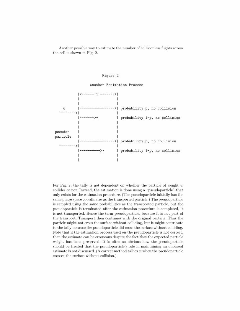
Another possible way to estimate the number of collisionless flights acrossthe cell is shown in Fig. 2.

Figure 2

Another Estimation Process

|<------ T ------->|| || |

w |----------------->| probability p, no collision-------->| |

|------->* | probability 1-p, no collision| || |

pseudo- | |particle | |

|----------------->| probability p, no collision-------->| |

|---------->* | probability 1-p, no collision| || |

For Fig. 2, the tally is not dependent on whether the particle of weight wcollides or not. Instead, the estimation is done using a “pseudoparticle” thatonly exists for the estimation procedure. (The pseudoparticle initially has thesame phase space coordinates as the transported particle.) The pseudoparticleis sampled using the same probabilities as the transported particle, but thepseudoparticle is terminated after the estimation procedure is completed, itis not transported. Hence the term pseudoparticle, because it is not part ofthe transport. Transport then continues with the original particle. Thus theparticle might not cross the surface without colliding, but it might contributeto the tally because the pseudoparticle did cross the surface without colliding.Note that if the estimation process used on the pseudoparticle is not correct,then the estimate can be erroneous despite the fact that the expected particleweight has been preserved. It is often so obvious how the pseudoparticleshould be treated that the pseudoparticle’s role in maintaining an unbiasedestimate is not discussed. (A correct method tallies w when the pseudoparticlecrosses the surface without collision.)

15.2 Preserving the Expected Weight is not Always a NecessaryCondition for an Unbiased Mean

The previous subsection showed that preserving the expected weight is notalways a sufficient condition for an unbiased mean. Now, it is shown thatpreserving the expected weight is not always a necessary condition for anunbiased mean. Experienced Monte Carlo practitioners correctly might sus-pect some legerdemain here. Consider Fig. 2 again. Inasmuch as the tallydepends (for the current transport step) not on the particle’s weight, but onthe weight associated with the pseudoparticle, the particle weight can be setto any arbitrary value, provided the particle weight is returned to w whenthe particle collides or crosses the surface. Thus, preserving the expectedweight is not necessary for this step in the transport process. With the tallynot responding to the original particle, one possible interpretation is that theparticle weight is zero for that step. Things will get even more curious in thenext subsection.

15.3 Multiple Particle Weights

Particle weight is normally conceived of as a single value for each particle. Notonly can one conceive of particles having multiple weights, multiple weightsare used in some production transport codes. Before jumping to the practicaluses of multiple weights, two simple examples are discussed.

Building on the previous two subsections, suppose that the code uses twodifferent estimators for the number of particles crossing the surface. The firstestimator uses the original particle as in Fig. 1 and the second estimator usesthe pseudoparticle as in Fig. 2. In this case, the original particle should haveweight w so that the first estimator is correct, but it can still have zero weightfor the second estimator. That is, the particle can have a different weight foreach estimator.

For another simple example, suppose that a particle of weight w reachesa surface as shown in Fig. 1. Upon crossing the surface, split the particle intotwo particles each of the original weight w. The total expected weight is notpreserved by this split, but unbiased estimates can again be made by a bitof legerdemain with the estimators. Label the particles 1 and 2. Label theestimators with positive integers. Let the odd numbered estimators respondonly to particle 1 and let the even numbered estimators respond only toparticle 2. This can be viewed as follows. The presplit particle contributed toall tallies and thus can be considered to have a weight vector (w,w). Afterthe split, particle 1 has weight vector (w, 0) and particle 2 has weight vector(0, w).

Turning to practical uses of multiple weights, note that perturbation andcorrelated sampling methods use different weights for the reference systemand the perturbed system. For example, Ref. [5, page 307] explicitly uses aweight vector in the discussion of correlated sampling.

The dxtran method in MCNP is very similar to the second example above.Upon surviving a collision, a particle is partitioned into two particles. The“dxtran particle” represents the uncollided particles that arrive on a userspecified dxtran sphere. The “nondxtran particle” represents the remainderof the particles. Note that the nondxtran particle has the original weight,w, at the collision exit point and the dxtran particle has a nonzero weight.Thus, the total particle weight is always larger than w at the collision exitpoint. The trick here is that the dxtran particle has zero weight for anytallies made before crossing the dxtran sphere and appropriate weight forany tallies afterward. Conversely, the nondxtran particle has weight w for alltallies made before crossing the dxtran sphere and zero weight for any talliesafterward.

Multiple weights can also be used to get low variance estimates for mul-tiple tallies. Consider a particle with a single weight in a slab penetrationproblem. Suppose the numbers of particles exiting the slab in the three en-ergy ranges 1.00 to 1.01, 1.01 to 1.02, and 1.02 to 1.03 MeV are desired. Notethat a zero variance sampling for the energy range 1.00 to 1.01 MeV meansthat every particle has to exit the slab within this energy range. This meansthat no particles exit in the other two energy ranges. Thus, a random walkprocess that gives a zero variance estimate for one energy range gives an in-finite variance estimate for all other energy ranges. Most of the sampling toget a zero variance solution in one interval is going to be very similar to thesampling to get a zero variance solution in either of the other two intervals. Itseems ridiculous that a zero variance solution in one interval forces an infinitevariance in the other intervals. Reference [14] shows that it is possible to getzero variance solutions in all three intervals at once using particles that carrythree weights. The method works by simultaneously applying several differ-ent importance functions, one for each tally, in a correlated way. Althoughzero variance estimates are impractical because the importance functions arenot known exactly, low variance solutions are possible with approximate im-portance functions. The method in [14] follows a single particle with multiplenonzero weights until the correlation between the importance functions de-creases enough that the particle must, statistically, execute different randomwalks for different tallies. (Curiously, Monte Carlo theories seem to focuson a single importance function despite the fact that multiple estimates areusually sought.)

16 Practical Variance Reduction

Designing practical variance reduction methods using solely an integral equa-tion approach is often problematical. First, the methods designed via anintegral equation approach almost always are weight independent methodsbecause weight dependent methods are not usually analyzed by integral equa-tions. Second, minimization of the variance in the transport process is usually

limited to making approximate use of zero variance biasing or optimizing afixed set of parameters associated with the method (e.g. see [5, chapter 7]).At the end of this optimization, one typically has some roughly optimized setof parameters that minimize the variance in a weight independent simulation.What one does not usually have is an understanding of the remaining sourcesof variance in the simulation after the optimization.

It may be that the variance reduction method, though optimized for theparticular set of parameters, is not treating some important source of vari-ance in the simulation. Consider, for example, neutron penetration of an ironslab. One can optimize the geometry splitting/roulette parameters in MCNP,but the calculation may still have a large source of variance associated withinadequate sampling of the iron cross section window at 24 kilovolts.

As a practical matter, it is usually important to understand the source ofany remaining variance in the problem. Unless one understands the sourceof the variance, it is difficult to know if any of a code’s standard variancereduction methods attack the source of the variance. Stated another way,once the source of the remaining variance cannot be attacked by any of thecode’s standard variance reduction techniques, then either

1. the user’s variance reduction efforts should end, or2. a new variance reduction method that attacks the source of the variance

must be implemented in the code

Fortunately, understanding the source of variance often is not too difficult.One finds the source particles that contributed most to the tally (MCNPdoes this automatically for the largest contribution) and one looks at thesesource particles in detail either via a printout for the particle (an “event log”in MCNP) or via a debugger. If one cannot find anything indicating poorsampling (e.g. hitting an iron window, streaming up a duct, or excessivelyhigh weights) then the simulation should be reasonably efficient. On the otherhand, if the particle having the largest tally is rare in the sense that it sampledan important pathway that almost all other particles miss, then the user canexamine the variance reduction methods in the code that might increase thesampling frequency for this rare pathway.

Note that many of the deficiencies in Monte Carlo variance reductiontechniques can be corrected by introducing weight dependent games. In thepast, the exponential transform at Los Alamos was often described as a “dialan answer technique” because the sample mean was sometimes extremelyunstable and often seemed to depend on what transform parameter was used.The weight window easily corrected this problem. The stratified splittinggame suggested in [4] sometimes was found to have a higher variance thanthe standard weight window splitting in MCNP. From a theoretical point ofview, it was difficult to understand why the stratified splitting game was worsethan the unstratified weight window splitting. After examining the stratifiedsplitting transport process by following a few particles around, the situationbecame clear. An analysis of the cause of the higher variance associated with

the stratified splitting technique pointed the way toward a small (weightdependent) modification of the technique that made the stratified splittingbetter than the weight window splitting[15].

As a practical matter, people need to pay attention to the sources of vari-ance in the transport process when considering variance reduction methods.

17 Comments on Theory and Tinkering

A person confronted with solving a Monte Carlo transport problem todayhas a variety of variance reduction techniques that can be applied in thevarious transport codes. The Monte Carlo literature tends to focus on vari-ance reduction techniques that have been analyzed using integral equations.Unfortunately, only a small fraction of MCNP calculations fit the cases de-scribed in the literature. The usual culprit, as indicated in numerous instancesherein, is the presence of weight dependent games in the MCNP calculations.More theory is needed for these weight dependent games. Weight dependentgames in MCNP seem to allow more efficient simulations than the weightindependent games described in the literature.

With the important exceptions of choosing weight windows or MCNP cellimportances, which can be obtained by stochastic methods (e.g. MCNP’sweight window generator) or sometimes deterministic methods (e.g. discreteordinates[16]), very little of the variance reduction is automatic. In practice,some MCNP users attempt variance reduction by tinkering. They tinker with-out looking at the transport process to determine the source of the variance.They tinker with different methods and they tinker with the parameters ofthe methods. Quite often, the tinkering is ineffective, for reasons explainedbelow.

With enough effort, the user empirically can optimize a set of parameters,but the optimum is only over the methods and sets of parameters chosen.Without investigating particles to determine what is causing the variance,the tinkering is essentially done in the dark, with the hope that the op-timum parameter selection will lead to an efficient calculation. Suppose, forinstance, that the user attempts to do a slab penetration problem using solelythe exponential transform. With enough tinkering, the user will presumablyarrive near the optimum transform parameter obtainable by references [8–11]. As mentioned in section 13, practical MCNP experience indicates thatthe exponential transform without a weight window gives a very inferior re-sult compared to the exponential transform with a weight window. Whetherthe optimum is theoretically derived or empirically derived, the calculationis missing weight control as a key factor in controlling the weight fluctua-tions introduced by the exponential transform technique. A quick look at theparticle history contributing the largest tally highlights the problem almostimmediately.

18 Summary

This report has noted some significant differences between the way MonteCarlo transport theory is normally presented and what MCNP actually does.Additionally, this report has tried to show that there is a significant valuein a transport process approach to variance reduction in MCNP. That is,MCNP users should understand not only the integral equation approach tovariance reduction, but the transport process approach as well. Note that thetwo approaches are not mutually exclusive. This report gives two examplesof useful techniques (i.e., stratified splitting and the exponential transform)that were developed based on transport equation considerations and thenwere improved by transport process considerations.

As a practical matter, MCNP users need to pay attention to the sources ofvariance in the transport process when considering variance reduction meth-ods. The cause of a high variance simulation in MCNP is not often apparentfrom a look at the transport equation; in contrast, the cause is often apparentafter examining the largest scoring particle histories.

Finally, this report (especially sections 14 and 15) encourages MCNP usersto take a broad view of Monte Carlo variance reduction.

AcknowledgementThough they do not necessarily agree with everything in this mansuscript,

the author wishes to acknowledge helpful comments and discussions withMalvin Kalos and Jerome Spanier.

References

1. X-5 Monte Carlo Team, “MCNP-A General Monte Carlo N-Particle TransportCode, Version 5,” Los Alamos National Laboratory Report LA-UR-03-1987,April 24, 2003

2. Jerome Spanier and Ely M. Gelbard, “Monte Carlo Principles and NeutronTransport Problems,” Addison-Wesley Publishing Company (1969).

3. Zero-Variance Solutions for Linear Monte Carlo, Thomas E. Booth, NuclearScience and Engineering: 102, 332-340 (1989)

4. Malvin H. Kalos and Paula A. Whitlock, “Monte Carlo Methods Volume I: Ba-sics,” John Wiley and Sons (1986).

5. Ivan Lux and Laszlo Koblinger, “Monte Carlo Particle Transport Methods: Neu-tron and Photon Calculations,” CRC Press, Inc. (1991).

6. Unbiased Combinations of Nonanalog Monte Carlo Techniques and Fair Games,Thomas E. Booth and Shane P. Pederson, Nuclear Science and Engineering: 110,254-261 (1992)

7. Bennett L Fox, “Strategies for Quasi-Monte Carlo,” Kluwer Academic Publish-ers 1999

8. An Analytic Approach to Variance Reduction, J. Spanier, SIAM J. Appl. Math.18 172 (1970)

9. A New Multistage Procedure for Systematic Variance Reduction in Monte Carlo,J. Spanier, SIAM J. Appl. Math. 18 172 (1970)

10. Optimal Choice of Parameters for Exponential Biasing in Monte Carlo, A. Dubiand Donald J. Dudziak, Nuclear Science and Engineering: 70, 1-13 (1979)

11. Prediction of Statistical Error and Optimization of Biased Monte Carlo Trans-port Calculations, P. K. Sarkar and M. A. Prasad Nuclear Science and Engi-neering: 70, 243-261 (1979)

12. A Sample Problem for Variance Reduction in MCNP, Thomas E. Booth LosAlamos National Lab. Report: LA-10363-MS, 1985 (available electronically viahttp://www-xdiv.lanl.gov/x5/MCNP/thedocumentation.html)

13. A Weight (Charge) Conserving Importance-Weighted Comb for Monte CarloT. E. Booth 1996 Radiation Protection and Shielding Division Topical Meeting,American Nuclear Society, N. Falmouth, MA, April 1996

14. Simultaneous Monte Carlo Zero-Variance Estimates of Several CorrelatedMeans, Thomas E. Booth, Nuclear Science and Engineering: vol 129, June 1998

15. Insights into Stratified Splitting Techniques for Monte Carlo Neutron Trans-port, Thomas E. Booth, Los Alamos Report LA-UR-03-5955, submitted to Nu-clear Science and Engineering

16. Wagner, J.C. and Haghighat, A., “Automated Variance Reduction of MonteCarlo Using the Discrete Ordinates Adjoint Function,” Nuclear Science andEngineering, Vol. 128,1998, pp. 186-208.