10 | Monopolistic Competition and Oligopoly Monopolistic Competition Oligopoly.
Upload
duongthienCategory
view
223download
0
A Theory of Dynamic Oligopoly, II: Price Competition, Kinked Demand Curves, andEdgeworth CyclesAuthor(s): Eric Maskin and Jean TiroleSource: Econometrica, Vol. 56, No. 3 (May, 1988), pp. 571-599Published by: The Econometric SocietyStable URL: http://www.jstor.org/stable/1911701Accessed: 10/09/2009 09:14
Your use of the JSTOR archive indicates your acceptance of JSTOR's Terms and Conditions of Use, available athttp://www.jstor.org/page/info/about/policies/terms.jsp. JSTOR's Terms and Conditions of Use provides, in part, that unlessyou have obtained prior permission, you may not download an entire issue of a journal or multiple copies of articles, and youmay use content in the JSTOR archive only for your personal, non-commercial use.
Please contact the publisher regarding any further use of this work. Publisher contact information may be obtained athttp://www.jstor.org/action/showPublisher?publisherCode=econosoc.
Each copy of any part of a JSTOR transmission must contain the same copyright notice that appears on the screen or printedpage of such transmission.
JSTOR is a not-for-profit organization founded in 1995 to build trusted digital archives for scholarship. We work with thescholarly community to preserve their work and the materials they rely upon, and to build a common research platform thatpromotes the discovery and use of these resources. For more information about JSTOR, please contact [email protected].
The Econometric Society is collaborating with JSTOR to digitize, preserve and extend access to Econometrica.
http://www.jstor.org
Econometrica, Vol. 56, No. 3 (May, 1988), 571-599
A THEORY OF DYNAMIC OLIGOPOLY, II: PRICE COMPETITION, KINKED DEMAND CURVES,
AND EDGEWORTH CYCLES
BY ERIC MASKIN AND JEAN TIROLE1
We provide game theoretic foundations for the classic kinked demand curve equilibrium and Edgeworth cycle. We analyze a model in which firms take turns choosing prices; the model is intended to capture the idea of reactions based on short-run commitment. In a Markov perfect equilibrium (MPE), a firm's move in any period depends only on the other firm's current price. There are multiple MPE's, consisting of both kinked demand curve equilibria and Edgeworth cycles. In any MPE, profit is bounded away from the Bertrand equilibrium level. We show that a kinked demand curve at the monopoly price is the unique symmetric "renegotiation proof" equilibrium when there is little discounting.
We then endogenize the timing by allowing firms to move at any time subject to short-run commitments. We find that firms end up alternating, thus vindicating the ad hoc timing assumption of our simpler model. We also discuss how the model can be enriched to provide explanations for excess capacity and market sharing.
KEiiwoRDs: Tacit collusion, Markov perfect equilibrium, kinked demand curve, Edge- worth cycle, excess capacity, market sharing, endogenous timing.
1. INTRODUCTION
MODELING PRICE COMPETITION has posed a major challenge for economic research ever since Bertrand (1883). Bertrand showed that, in a market for a homogeneous good where two or more symmetric firms produce at constant cost and set prices simultaneously, the equilibrium price is competitive, i.e., equal to marginal cost. This classic result seems to contradict observation in two ways. First, in markets with few sellers, firms apparently do not typically sell at marginal cost. Second, even in periods of technological and demand stability, oligopolistic markets are not always stable. Prices may fluctuate, sometimes wildly.
Of course, one reason for these discrepancies between theory and evidence is that the Bertrand model is static, whereas dynamics may be an important ingredient of actual price competition.2 Indeed, two classic concepts in the industrial organization literature, the Edgeworth cycle and the kinked demand curve equilibrium, offer dynamic alternatives to the Bertrand model.
In the Edgeworth cycle story, firms undercut each other successively to increase their market share (price war phase) until the war becomes too costly, at which point some firm increases its price. The other firms then follow suit (relenting phase), after which price cutting begins again. The market price thus
1 We thank David Kreps, Robert Wilson, two referees, and especially John Moore, for very helpful comments. This work was supported by the Sloan Foundation and the National Science Foundation.
2 Another possible explanation for lack of perfect competition-indeed, the most common theoretical one-is that products of different firms are not perfect substitutes. Alternatively, as Edgeworth (1925) suggested, firms may be capacity-constrained.
571
572 ERIC MASKIN AND JEAN TIROLE
evolves in cycles. The concept is due to Edgeworth (1925), who, in his criticism of Bertrand, showed that static price equilibrium does not in general exist when firms face capacity constraints. His resolution of this nonexistence problem was the cycle.
By contrast with the Edgeworth cycle, the market price for a kinked demand curve (Hall and Hitch (1939), Sweezy (1939)) is stable in the long run. This "focal" price is sustained by each firm's fear that, if it undercuts, the other firms will do so too. A firm has no incentive to charge more than the focal price because it believes that, in that case, the other firms will not follow.
Despite their long history, the Edgeworth cycle and kinked demand curve have received for the most part only informal theoretical treatments. The primary purpose of this paper is to provide equilibrium foundations for these two types of dynamics.
The basis of our analysis is a model of duopoly where firms take turns choosing prices (see Section 2). The alternating move assumption is meant to capture the idea of short-run commitment; see our companion piece for motivat- ing discussion. A firm maximizes the present discounted value of its profit. Its strategy is assumed to depend only on the physical state of the system (i.e., to be Markov). In our model, the state is simply the other firm's current price.
We first show through examples that an equilibrium of this model may be a kinked demand curve or a price cycle3 (Section 3). Section 4 examines the general nature of equilibrium in our model. In particular, it establishes that any equi- librium must be either of the kinked demand type (where the market price converges in finite time to a unique focal price) or the Edgeworth cycle variety (in which the market price never settles down).
Section 5 proves that there exists a multiplicity of kinked demand curve equilibria. Specifically, we exhibit the exact range of possible equilibrium focal prices when the discount factor is near 1. This range-a closed interval contain- ing the monopoly price-lies well above the competitive price. We argue in Section 6, however, that only one of these-the monopoly price equilibrium (which is unique)-is "renegotiation proof" in the sense that firms would never find it to their advantage to move to another equilibrium. We go on to investigate firms' adjustment to stochastic shifts in demand, showing, in particular, that an increase in demand may well trigger a price war.
Section 7, which treats Edgeworth cycles, is the counterpart of Section 5 on kinked demand curves. It demonstrates, by construction, the existence of Edge- worth cycle equilibria if the discount factor is sufficiently near 1 and proves that, in any such symmetric equilibrium, average aggregate profit must be no less than half the monopoly level.
In Section 8 we compare the qualitative nature of equilibrium in this paper with that of Part I of our study, which models competition in quantities/capaci- ties. Whereas here there are many equilibria, symmetric equilibrium is unique in the companion paper. The respective comparative statics, moreover, are com-
3Unlike Edgeworth's treatment, price cycles in our model do not rely on capacity constraints.
DYNAMIC OLIGOPOLY, II 573
pletely opposed. These contrasts can be traced to differences in the behavior of the cross partial derivative of the instantaneous profit function.
We acknowledge in Part I of this study that a model where firms' relative timing is imposed is unduly artificial. Accordingly, in Section 9, we show that the fixed timing analysis through Section 7 continues to hold when embedded in either of the endogenous timing frameworks discussed in our companion piece.
Our modeling methodology contrasts sharply with that of the well-established supergame model of tacit collusion. In Section 10 we draw a detailed comparison between the two approaches.
Finally, in Section 11, we discuss how our model can be extended to accom- modate competition in quantities as well as prices. In particular, we provide explanations of two prominent market phenomena: excess capacity and market sharing.
2. THE MODEL
In this section we describe the main features of the exogeneous-timing duopoly model. Competition between the two firms (i = 1,2) takes place in discrete time with an infinite horizon. Time periods are indexed by t (t = 0,1, 2,...). The time between consecutive periods is T. At time t, firm i's instantaneous profit g1 is a function of the two firms' current prices pl and p2, but not of time: 7Tr= Ti( pt, p7). We will assume that the goods produced by the two firms are perfect
substitutes, and that firms share the market equally when they charge the same price. The price space is discrete, i.e., firms cannot set prices in units smaller than, say, a penny.4 In most of the paper we assume that firms have the same unit cost c. Letting D(.) denote the market demand function, define
(1) II(p)-(p-c)D(p).
The total profit function 1(p) is assumed to be strictly concave. Let pm denote the monopoly price, i.e., the value of p maximizing (1). From our assumptions,
(11(pi), if pt, pJ
'rr'(pl, pt) H(p,)/2, if p;=pj,
0, if p; >Pt.
Firms discount the future with the same interest rate r; thus their discount factor is 8 exp (-rT). Because one expects that ordinarily firms can change prices fairly quickly, we will often think of T as being small and, therefore, of 8 as being close to one. Firm i's intertemporal profit at time t is
00
E SSIi(pi p2)
s=O
4 The reason for this restriction is to ensure that optimal reactions exist. In a static Bertrand model, for example, best responses to prices above marginal cost are not defined when the price space is a continuum.
574 ERIC MASKIN AND JEAN TIROLE
As in our companion paper, we begin by assuming that firms move alternately. In odd-numbered periods t, firm 1 chooses its price, which remains unchanged until period t + 2. That is, p?i = p1 if t is odd. Similarly, firm 2 chooses prices only in even-numbered periods, so that P2 1 = p2 if t is even. As in Part I, we impose the Markov assumption: a firm's strategy depends only on the payoff-rel- evant state, those variables that directly enter its payoff function. In our model, the payoff-relevant state is just the price the other firm set last period. Hence, firm i's strategy is a dynamic reaction function, a (possibly random) function R'(.), where pt = R( ptt- 1) is the firm's price in period t given that the other firm set pt 1 in period t-1.
We are interested in Markov perfect equilibria (MPE): pairs of dynamic reaction functions forming perfect equilibria. From dynamic programming5 (see Maskin-Tirole (1988) for details), a pair (R1, R2) is an MPE if, for all prices fp,
(2) v1(p) = max [1(p, ) + w(p)], p
and
(3) W1( =Ep[ 1(p, p) + S(p)]
where R1( p) is a maximizing choice of p in (2), the expectation in (3) is taken with respect to the distribution of R2( p), and where the symmetric conditions hold for firm 2. The expression, V'(p) is firm i's valuation (present discounted profit) if (a) it is about to move, (b) the other firm's current price is p, and (c) firms henceforth play according to (R1, R2). The expression Wi(p) is firm i's valuation if last period it played p, the other firm is about to move, and firms use (R1, R2) forever after.
Most of our results will be demonstrated for discount factors close to one, which, as we already suggested, is often a reasonable assumption for price competition. Thus, a typical proposition will hold for all 8 greater than a given 8 < 1. We sometimes also require the set of possible prices to be sufficiently " fine."
3. KINKED DEMAND CURVES AND EDGEWORTH CYCLES: EXAMPLES
This section exhibits two examples of Markov Perfect Equilibria, one a "kinked demand curve," the other an "Edgeworth cycle." In both examples the market demand curve is given by D (p) = 1 -p, and production is costless. Firms can charge any of seven prices: p(i) = i/6 for i = 0,1, . . ., 6. The corresponding profits, I( p(i)) = p(i)(1 - p(i)) are proportional, respectively, to 0, 5, 8, 9, 8, 5, 0. The monopoly price is ptm = p(3) = 1/2.
Suppose that dynamic reaction functions are symmetric and described by Table I, where /3(3) (5 + 8)/(58 + 932)
5 Because the set of available prices is finite, the instantaneous profit functions are bounded, which is sufficient for dynamic programming to be applicable.
DYNAMIC OLIGOPOLY, II 575
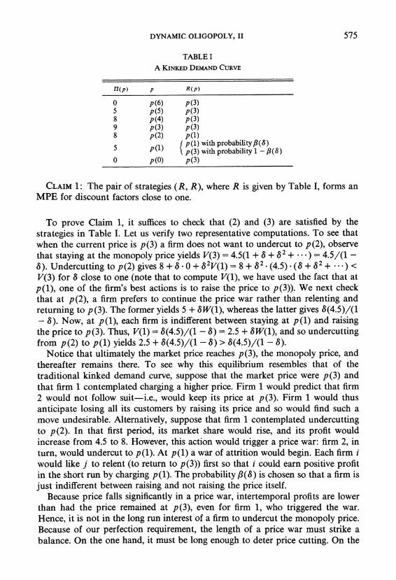
TABLE I
A KINKED DEMAND CURVE
11(p) p R(p)
O p(6) p(3) 5 p(5) p(3) 8 p(4) p(3) 9 p(3) p(3) 8 p(2) p(l) 5 1
( p(l) with probability ?(8) "'i) ' p(3) with probability 1 - fl(8)
0 p(O) p(3)
CLAIM 1: The pair of strategies (R, R), where R is given by Table I, forms an MPE for discount factors close to one.
To prove Claim 1, it suffices to check that (2) and (3) are satisfied by the strategies in Table I. Let us verify two representative computations. To see that when the current price is p(3) a firm does not want to undercut to p (2), observe that staying at the monopoly price yields V(3) = 4.5(1 + 8 + 82 + ** * ) = 4.5/(1 - 8). Undercutting to p(2) gives 8 + S. 0 + 82V(1) = 8 + 832 _(4.5) .(3 + 832 + * - ) < V(3) for 8 close to one (note that to compute V(1), we have used the fact that at p(l), one of the firm's best actions is to raise the price to p(3)). We next check that at p(2), a firm prefers to continue the price war rather than relenting and returning to p(3). The former yields 5 + 3W(1), whereas the latter gives 8(4.5)/(1 - 8). Now, at p(l), each firm is indifferent between staying at p(l) and raising the price to p(3). Thus, V(1) = 8(4.5)/(1 - 8) = 2.5 + 3W(1), and so undercutting from p(2) to p(l) yields 2.5 + 8(4.5)/(1 - 8) > 8(4.5)/(1 - 8).
Notice that ultimately the market price reaches p(3), the monopoly price, and thereafter remains there. To see why this equilibrium resembles that of the traditional kinked demand curve, suppose that the market price were p(3) and that firm 1 contemplated charging a higher price. Firm 1 would predict that firm 2 would not follow suit-i.e., would keep its price at p(3). Firm 1 would thus anticipate losing all its customers by raising its price and so would find such a move undesirable. Altematively, suppose that firm 1 contemplated undercutting to p(2). In that first period, its market share would rise, and its profit would increase from 4.5 to 8. However, this action would trigger a price war: firm 2, in turn, would undercut to p(l). At p(l) a war of attrition would begin. Each firm i would like j to relent (to return to p(3)) first so that i could earn positive profit in the short run by charging p(l). The probability /(3) is chosen so that a firm is just indifferent between raising and not raising the price itself.
Because price falls significantly in a price war, intertemporal profits are lower than had the price remained at p(3), even for firm 1, who triggered the war. Hence, it is not in the long run interest of a firm to undercut the monopoly price. Because of our perfection requirement, the length of a price war must strike a balance. On the one hand, it must be long enough to deter price cutting. On the
576 ERIC MASKIN AND JEAN TIROLE
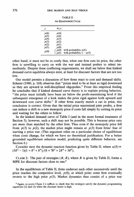
TABLE II
AN EDGEWORTH CYCLE
p R(p)
p(6) p(4) p(5) p(4) p(4) p(3) p(3) p(2) p(2) p(l) p(l) p(O)
p(O) f p(O) with probability a(8) \ p(5) with probability 1 - a(8)
other hand, it must not be so costly that, when one firm cuts its price, the other firm is unwilling to carry on with the war and instead prefers to relent im- mediately. Despite these conflicting requirements, we shall see below that kinked demand curve equilibria always exist, at least for discount factors that are not too low.
Our model permits a discussion of how firms react to cost and demand shifts. Scherer (1980, p. 168) observes that "prices tend to be at least as rigid downward as they are upward in well-disciplined oligopolies." From this empirical finding he concludes that if kinked demand curve theory is to explain pricing behavior, ""the price must initially have been set below the profit-maximizing level if the subsequent emergence of a kink makes the price rigid against both upward and downward cost curve shifts." If other firms exactly match a cut in price, this conclusion is correct. Given that the initial price maximized joint profits, a firm can induce a shift to a new monopoly price if costs fall simply by cutting its price and waiting for the others to follow.
In the kinked demand curve of Table I (and in the more formal treatment of Section 5), however, such a shift may not be possible. This is because price cuts are more than matched by the other firm. Thus even if the monopoly price fell from p(3) to p(2), the market price might remain at p(3) from firms' fear of starting a price war. (This argument relies on a particular choice of equilibrium when costs change, for which we have no theoretical justification. For a better grounded equilibrium selection model, predicting quite different behavior, see Section 6.)
Consider next the dynamic reaction function given by Table II, where a(8) (3382 _ 1)(1 + 82 + 84)/(8 + 782 + 284 + 386).
CLAIM 2: The pair of strategies (R, R), where R is given by Table II, forms a MPE for discount factors close to one.6
In the equilibrium of Table II, firms undercut each other successively until the price reaches the competitive level, p(0), at which point some firm eventually reverts to the high price p(5). Market dynamics thus consist of a price war
6Again, to prove Claim 2 it suffices to check that the strategies satisfy the dynamic programming equations (2) and (3) when the discount factor is high.
DYNAMIC OLIGOPOLY, II 577
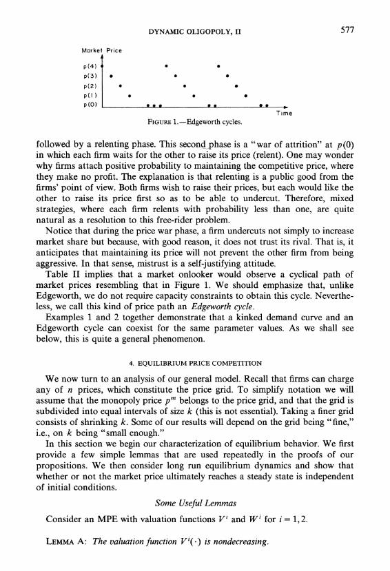
Market Price
p(4) S
p(3) * * 0
p(2) * 0
p(l)
p(O) . s*
Time FIGURE 1.-Edgeworth cycles.
followed by a relenting phase. This second -phase is a "war of attrition" at p (0) in which each firm waits for the other to raise its price (relent). One may wonder why firms attach positive probability to maintaining the competitive price, where they make no profit. The explanation is that relenting is a public good from the firms' point of view. Both firms wish to raise their prices, but each would like the other to raise its price first so as to be able to undercut. Therefore, mixed strategies, where each firm relents with probability less than one, are quite natural as a resolution to this free-rider problem.
Notice that during the price war phase, a firm undercuts not simply to increase market share but because, with good reason, it does not trust its rival. That is, it anticipates that maintaining its price will not prevent the other firm from being aggressive. In that sense, mistrust is a self-justifying attitude.
Table II implies that a market onlooker would observe a cyclical path of market prices resembling that in Figure 1. We should emphasize that, unlike Edgeworth, we do not require capacity constraints to obtain this cycle. Neverthe- less, we call this kind of price path an Edgeworth cycle.
Examples 1 and 2 together demonstrate that a kinked demand curve and an Edgeworth cycle can coexist for the same parameter values. As we shall see below, this is quite a general phenomenon.
4. EQUILIBRIUM PRICE COMPETITION
We now turn to an analysis of our general model. Recall that firms can charge any of n prices, which constitute the price grid. To simplify notation we will assume that the monopoly price pm belongs to the price grid, and that the grid is subdivided into equal intervals of size k (this is not essential). Taking a finer grid consists of shrinking k. Some of our results will depend on the grid being "fine," i.e., on k being "small enough."
In this section we begin our characterization of equilibrium behavior. We first provide a few simple lemmas that are used repeatedly in the proofs of our propositions. We then consider long run equilibrium dynamics and show that whether or not the market price ultimately reaches a steady state is independent of initial conditions.
Some Useful Lemmas
Consider an MPE with valuation functions V' and W' for i = 1,2.
LEMMA A: The valuation function Vi(-) is nondecreasing.
578 ERIC MASKIN AND JEAN TIROLE
PROOF: For convenience, suppose that i = 1. Consider two prices p <p3. Let p belong to the support of R1(p). We have
(p) =1p p) p p + W1(p)
where the first inequality follows from the fact that a firm's profit is nondecreas- ing in its opponent's price, and the second inequality from the fact that A is a feasible reaction to p. Q.E.D.
A price is "focal" for a pair of strategies if, once it is set, firms continue to charge it forever. Thus a focal price pf satisfies
pf=Rl(pf) =R2(pf).
LEMMA B: If p f is focal price, then H(p f ) > .
PROOF: Suppose that, starting from pf, firm 1, say, raises its price to p >pf, where 1(p)> 0. If, contrary to the Lemma, I1(pf) < 0 (in which case Vl(pf) = V2( pf) < 0), the existence of p (we will handle the case where no such p exists below) implies that pf < pm and so Il(p) < 0 for all - f Because firm 2 has the option of reacting to p with p itself, V2(p) > 0. If, in fact, it reacts with a price below pf (it cannot react with pf since it would then earn nonpositive profit), it would therefore profit from cutting its price at pf, a contradiction. Thus, there exists a price A
> pf with 1(p) > 0 such that with positive probabil- ity firm 2 reacts to p with p. (If for all p such that H(p) > 0, H(p) < 0 for all p in R2(p), then V2(p) < 0 for all such, p, a contradiction.) But then firm 1 can earn positive profit by also playing p, and so raising its price to p guarantees it positive expected profit. Thus I(pf) >0.
If the firm cannot raise its price to p where 17(p) > 0, then pf > pm. In this case, however, the firm can always undercut and make a positive profit. Q.E.D.
For an equilibrium pair of dynamic reaction functions (R1, R2), a semi-focal price is a price pf such that pf is in the support of both Rl(pf) and R2(pf).
LEMMA C: If H(pf)> 0, a firm never reacts to a price p above a focal or semi-focal price, p f, by undercutting to a price p < pf or by raising its price. Thus the support of Ri(p) lies in the interval [pf, p].
PROOF: Let pf be a focal (or semi-focal) price. Assume that firm i reacts to p > p f by charging p < p f. We have
1(p) + 3Wj(A) > H(pf) + w(pf) since firm i could have undercut to pf. But pf is a semi-focal price. Thus, firm i does not gain by undercutting to p when the other firm charges pf:
(p) + 2wr(p + ) wi(pf
But these two inequalities are inconsistent if 1(pf) > 0.
7 I.e., pf exceeds marginal cost but is not so high as to choke off demand.
DYNAMIC OLIGOPOLY, II 579
Imagine next that, for some i, there exists b e R'( p) with p > p > pf. Since firm i could instead have set pf, we have:
swi(p) ? 11(pf) + wi( pf ),
which implies that
FI(pf) swi(i), >
2 + swi(pf)2
But this implies that pf is not a semi-focal price, since it tells us that at pf it is in firm i's interest to raise the price to p. Q.E.D.
Ergodic Equilibrium Behavior
Consider (possibly mixed) strategies R' and R2. In any period the market can be in any of 2n states. A state specifies (a) the firm that is currently committed to a price and (b) the price to which it is committed. The Markov strategies induce a Markov chain in this set of states. Let Xhg(t) denote the t-step transition probability between states h and g for this Markov chain. The states h and g (with h possibly equal to g) communicate if there exist positive t1 and t2 such that xgh(tl) > 0 and Xhg(t2) > 0. An ergodic class is a maximal set of states each pair of which communicate (see, e.g., Derman (1970)). A recurrent state is a member of some ergodic class.
Rather than considering states, we focus on the market price, the minimum of the two prices in a given period. The market price does not form a Markov chain, but, abusing terminology, we shall refer nonetheless to recurrent market prices and ergodic classes of market prices. A set of prices forms an ergodic class of market prices if it corresponds to an ergodic class of states.8 A recurrent market price is a member of an ergodic class.
We are interested in long run properties of Markov perfect equilibria, i.e., in their ergodic classes. An MPE is a kinked demand curve equilibrium if it has an ergodic class consisting of a single price9 (a "focal ergodic class"); it is an Edgeworth cycle equilibrium if it has an ergodic class of market prices that is not a singleton ("Edgeworth ergodic class").
A natural first question is whether an MPE can have several ergodic classes. This question is partially answered by Propositions 1 and 2.
8 Formally, let P(h) denote the set of potential market prices when the state is h (remember that mixed strategies are allowed). A set P of prices is an ergodic set of market prices if and only if there exists a set of states H such that (i) H is an ergodic set of states and (ii) P = Uh ,E H P(h).
9 We have labelled an MPE with a singleton ergodic class a "kinked demand curve equilibrium" because, as in the classic concept, no firm will wish to deviate from the focal price and because any such equilibrium has at least some of the salient properties of the example of Table I (whether it has all such properties remains an open question). As we shall see below (Propositions 1 and 2) each such MPE (for 8 near 1) does share the attractive feature of the example that, regardless of the starting point the market price eventually winds up at a unique steady-state pf (the focal price). Moreover, Lemma C ensures that a firm will react to a price p above pf with a price between p and pf. We conjecture that there always exists a price p < pf such that, at a price between p and pf, a firm undercuts but that at prices below p, the firm raises its price to a level not less than p1.
580 ERIC MASKIN AND JEAN TIROLE
PROPOSITION 1: For a given price grid, an MPE cannot have two focal ergodic classes if the discount factor is close enough to 1.
PROOF: Consider a fixed price space. First note that, if n( pl) 0 nI( P2), Pl and P2 cannot both be focal prices for a given MPE if 8 is sufficiently close to 1, as it would be in either firm's interest to jump to the high profit from the low profit focal price. Assume therefore that Pi and P2 are focal prices for which MI(PO) = (P2). If Pi <P2 then, at P2, a firm gains from reducing its price to Pi since it thereby gets the whole market to itself for one period (from Lemma B, l(pi) >0). Q.E.D.
PROPOSITION 2: An MPE cannot possess both a focal and an Edgeworth ergodic class.
PROOF: Suppose that an MPE has both a focal price pf and an Edgeworth ergodic class P. Let p be the highest price in P (recall that P is bounded). Because P is ergodic, there exist p e P (p <fi) and firm i such that
(8) - is in the support of R( p).
If p > p f, then P lies entirely above pf; otherwise, at some price in P above p f, one of the firms will undercut to a price below pf, a contradiction of Lemma C. But if P lies above pf, then (8) also contradicts Lemma C. Thus -
<pf.
For the firm i satisfying (8),
(9) sri(
>anpf)
because it could have reacted to p by setting pf. But because pf is a focal price, firm i does not gain by lowering its price from pf to p:
ii(pf ) (10) 2(1 - 8) > (p) + swi(p).
Inequalities (9) and (10) imply that
(11) IH(pf) > 2H(p),
which in turn implies that p is lower than pm (otherwise, from the strict quasi-concavity of n, P would exceed pf). Now, in the class P, the market price is never above p. Therefore,
> W(P),
which, with (9), implies that
2a(pn o (pf),
a contradiction of (11). Q.E.D.
DYNAMIC OLIGOPOLY, II 581
We have not yet been able to prove that an MPE cannot possess two Edgeworth ergodic classes. But Propositions 1 and 2 show that, in any case, Markov perfect equilibria can be subdivided into two categories that are indepen- dent of initial conditions. In one category, the market price converges in finite time to a focal price. In the other, the market price never settles down.
Actually, we believe that the structure of Edgeworth cycle equilibria can be made more precise. As currently defined, an Edgeworth cycle is simply an equilibrium without a focal price. We conjecture that in any Edgeworth cycle with a sufficiently fine grid, there exist prices
- and p (p <p) such that, for any
p>p, Ri(p)=p; and for anype(p,p], p <R'(p)<p.
5. KINKED DEMAND CURVES: GENERAL RESULTS
In this section we completely characterize equilibrium focal prices (i.e., the steady-states of kinked demand curve equilibria) for fine grids and high discount factors. We first define two prices x and y (x < pm <y) that will play a crucial role in this characterization. Let x and y be the elements of the price grid (recall that pm belongs to the price grid) such that
[I(x) > Ji(pm) > rI(x-k) and x <pm and
HI(y) >2HI(pm)>FI(y+k) and y>pm.
Thus profits at x and y are approximately four sevenths and two thirds of monopoly profit. We now study the set of prices that are focal prices of some MPE. This set is characterized in two steps.
PROPOSTION 3 (Necessary Conditions): If pf is a focal price of some MPE, then for a high discount factor, (i) pf < y; (ii) and for a sufficiently fine grid, pf> x.
PROPOSITION 4 (Sufficient Conditions): For a given (sufficiently fine) grid and a price p belonging to this grid and to the interval [x, y], p is the focal price of some MPE for a discount factor near one.
Propositions 3 and 4 determine the set of possible focal prices for fine grids when firms place sufficient weight on the future. We should emphasize two aspects of this characterization. First, focal prices are bounded away from the competitive price (zero profit level); firms must make at least four-sevenths of the monopoly profit in equilibrium. Second, there is a nondegenerate interval of prices that can correspond to a kinked demand curve equilibrium. This multiplic- ity accords well with the informal story behind the kinked demand curve. As this story is usually told, if other firms imitate price cuts but do not imitate price rises, a firm's marginal revenue curve will have a discontinuity at the current price. As long as the marginal cost curve passes through the interval of discon- tinuity, the current price can be an equilibrium (see Scherer (1980)).
582 ERIC MASKIN AND JEAN TIROLE
For complete proofs of these propositions, see Maskin-Tirole (1985). Here we attempt only to elucidate some of the ideas underlying Proposition 3 (see the Appendix for a sketch of a proof of Proposition 4).
PROOF OF PROPOSITION 3(i): That a focal price must not exceed y is readily seen. Remaining at pf yields profit I( pf)/2(1 - 8). If pf exceeds y, undercut- ting to the monopoly price yields at least n1(pm) + 831( pf )/2(1 - 8), because the undercutting firm can always move the market price back to the steady state by returning to pf two periods hence. Thus, for equilibrium, we have:
1H(pf)(j + 8 + 82)> J(pm)
which means that for 8 near 1, a focal price above the monopoly price must yield at least two-thirds the monopoly profit.
PROOF OF PROPOSITION 3(ii): We shall content ourselves with showing that in a pure strategy MPE (where each RK is deterministic), a focal price pf below pm must yield at least two-thirds the monopoly profit (allowing for mixed strategies reduces the lower bound to four-seventhsl). Let us fix the price grid, i.e., the interval k between prices. With pure strategies, Lemma C implies that
(12) for p>pfandIl(p)>Il(pf), Ri(p)<p i=1,2
(if Ri(p) =p for some i, firm j can guarantee itself 3I1(p)/2(l-3)> I(pf)/2(l - 3) for 8 close to 1, by relenting from pf to p and staying at p forever, and hence pf is not a focal price). Suppose, to the contrary, that 1n(pf) < (2/3)I1I(pm). Let
- >pf be the smallest price such that
(13) ( > p + )
i.e.,
(14) H(p)+82 ii(pf) >3 1pf)+ iH(pf)
For a fine enough grid, (13) implies that - E (pf pm). We claim first that
(15) RL(p) =pf for all p E(pf, ], i = 1,2.
Suppose to the contrary that there existed a price violating (15). Let p be the smallest such price. Then pf < Ri( p) < p for some i, implying
(16) vi( P) = In(Ri(p)) + 3211(pf) 2(1-38)
10 This is because mixing allows the possibility of semi-focal prices. Consider an MPE where pf is a focal price and p( > pf ) is a semi-focal price. If, at pf, a firm should raise its price to p or above, the market price eventually returns to pf. Suppose, however, we ruled out mixing. Then p would have to be a full-fledged focal price itself, and thus the market price, once raised above p, would not return to pf. The fact that the market price would remain at p would give a firm a greater incentive to raise its price. Thus pf cannot be as low in a pure strategy as in a mixed strategy MPE.
DYNAMIC OLIGOPOLY, II 583
By definition of p, V'(pl) is less than the right side of (13), a contradiction since the firm could always choose the price pt. Hence, (15) holds.
Now, in view of (15) and the definition of p, R1(p + k) cannot lie in (p p) because firm i would do better to charge price pf. But, from (13), it does still better to charge p. Hence
(17) R'(p+k)=p, i=1,2.
We next argue that
(18a) R'(-+2k)=-+k, i=152.
From the above argument, R1(p + 2k) E {p, - + k}. Now, if, at - + 2k, firm i cuts its price to p, its profit is
8211(pf)
(p) 2(1-8)
However, if, instead, it reduces its price to p + k, (17) implies that its profit is
II(p + k) + 32(H(pf) + 2(1 - 8) )
which is bigger. Hence, (18a) holds. Similarly
(18b) R{ - +3k)=-+2k.
Because pf is a focal price,
vJi(pf)- i(f), i=1,2. 2(1 -a8) However, if, at pf, firm i raises its price to - + 3k, (17), (18a), and (18b) imply that its payoff is no less than
8 2I ( - + k ) + 84 ( pf ) + sri( pf) 32(3k+31(t+2(1 -a8)
which, from (14), is greater than V'(pf) for 8 near 1, a contradiction. Thus, as long as the grid is fine enough so that
- + 3k < pm, pf > x for 8 near 1. Q.E.D.
Although this proof of the second part of Proposition 3 applies only to pure strategies, it should convey the intuition behind the result. If a putative price pf is too low, a firm does better by raising its price well above pf. If it does so, it can ensure that the price remains high long enough for it to recoup the loss it suffers from raising its price first.
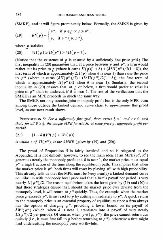
When the focal price is pm, there is a particularly simple kinked demand curve equilibrium in which each firm (i) cuts its price to pm when the market price is above pm, (ii) cuts its price immediately to a relenting price p when the market price is between p and pm; and (iii) raises its price to pm when the-price is below p. We shall call this the simple monopoly kinked demand curve equilibrium
584 ERIC MASKIN AND JEAN TIROLE
(SMKE), and it will figure prominently below. Formally, the SMKE is given by
pm, ifp < porp>,-pm, (19) R*(P)= p, if p E (p, pm),
where p satisfies
(20) 4rI(-p) >, H(pm) > 4-I(p p-k).
(Notice that the existence of p is ensured by a sufficiently fine price grid.) The first inequality in (20) guarantees that, at a price between p and pm, a firm would rather cut its price to p (where it earns Il(p)(1 + 8) + (82H1(pm)/2(1 - 8)), the first term of which is approximately 2Il(p) when 8 is near 1) than raise the price to pm (where it earns (3S1(pm)/2) + (8211(pm)/2(1 - 8)), the first term of which is approximately If(pm)/2 when 8 is near 1). Similarly, the second inequality in (20) ensures that, at p or below, a firm would prefer to raise its price to ptm than to undercut, if 8 is near 1. The rest of the verification that the SMKE is an MPE proceeds in much the same way.
The SMKE not only sustains joint monopoly profit but is the only MPE, even among those outside the kinked demand curve class, to approximate this profit level, as our next result shows.
PROPOSITION 5: For a sufficiently fine grid, there exists 8 < 1 and E > 0 such that, for all 8 > 8, the unique MPE for which, at some price p, aggregate profit per period
(21) (1 - 8)(Vi(p) + W'(p))
is within E of 17(pm), is the SMKE (given by (19) and (20)).
The proof of Proposition 5 is fairly involved and so is relegated to the Appendix. It is not difficult, however, to see the main idea. If an MPE (R', R2) generates nearly the monopoly profit and 8 is near 1, the market price must equal pm a high fraction of the time along the equilibrium path. This implies that when the market price is pm, both firms will react by playing pm with high probability. This already tells us that the MPE must be (very nearly) a kinked demand curve equilibrium with monopoly focal price and that a firm's payoff per period is very nearly Il( pm)/2. The reason equilibrium takes the form given by (19) and (20) is that these strategies ensure that, should the market price ever deviate from the monopoly level, it will return to pm quickly. Thus, for example, when the market price p exceeds pm, firms react to p by cutting immediately to pm. A quick return to the monopoly price is an essential property of equilibrium since a firm always has the option of charging pm, providing a lower bound on its payoff of SWi(pm) (which, when 8 is near 1, translates into a payoff of very nearly I17(pm)/2 per period). Of course, when p E (p, pm), the price cannot return too quickly (i.e., it must first fall to p before returning to pm), otherwise a firm might find undercutting the monopoly price worthwhile.
DYNAMIC OLIGOPOLY, II 585
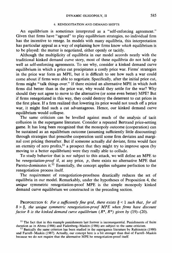
6. RENEGOTIATION AND DEMAND SHIFTS
An equilibrium is sometimes interpreted as a "self-enforcing agreement." Given that firms have "agreed" to play equilibrium strategies, no individual firm has the incentive to renege. In models with many equilibria, this interpretation has particular appeal as a way of explaining how firms know which equilibrium is to be played: the matter is negotiated, either openly or tacitly.
Although the multiplicity of equilibria in our model accords neatly with the traditional kinked demand curve story, most of these equilibria do not hold up well as self-enforcing agreements. To see why, consider a kinked demand curve equilibrium in which a price cut precipitates a costly price war. Firms' strategies in the price war form an MPE, but it is difficult to see how such a war could come about if firms were able to negotiate. Specifically, after the initial price cut, firms might "talk things over." If there existed an alternative MPE in which both firms did better than in the price war, why would they settle for the war? Why should they not agree to move to the alternative (or some even better) MPE? But if firms renegotiated in this way, they could destroy the deterrent to cut prices in the first place. If a firm realized that lowering its price would not touch off a price war, it might find such a cut advantageous. Hence, our kinked demand curve equilibrium would collapse.
The same criticism can be levelled against much of the analysis of tacit collusion in the supergame literature. Consider a repeated Bertrand price-setting game. It has long been recognized that the monopoly outcome (cooperation) can be sustained as an equilibrium outcome (assuming sufficiently little discounting) through strategies that prescribe cooperation until some firm deviates and margi- nal cost pricing thereafter. But if someone actually did deviate, firms would face an eternity of zero profits,11 a prospect that they might try to improve upon (by moving to a better equilibrium) were they really able to collude.
To study behavior that is not subject to this attack, we will define an MPE to be renegotiation-proof if, at any price, p, there exists no alternative MPE that Pareto-dominates it."2 Essentially, the concept applies subgame perfection to the renegotiation process itself.
The requirement of renegotiation-proofness drastically reduces the set of equilibria in our model. Remarkably, under the hypotheses of Proposition 4, the unique symmetric renegotiation-proof MPE is the simple monopoly kinked demand curve equilibrium we constructed in the preceding section.
PROPOSITION 6: For a sufficiently fine grid, there exists 8 < 1 such that, for all 8 > 3. the unique symmetric renegotiation-proof MPE when firms have discount factor 8 is the kinked demand curve equilibrium (R*, R*) given by (19)-(20).
" The fact that in this example punishments last forever is inconsequential. Punishments of finite duration as in Abreu (1986) and Fudenberg-Maskin (1986) are subject to the same criticism.
12 Basically the same criterion has been studied in the supergames literature by Rubinstein (1980) and Farrell-Maskin (1987). Actually, our concept here is a bit stronger than that of Farrell-Maskin because we do not require that the alternative MPE be renegotiation-proof itself.

586 ERIC MASKIN AND JEAN TIROLE
PROOF: For 8 near 1 and any price p,
(22) (1 - 8)(V*(p) + W*(p)) = (p ),
where V* and W* are the valuation functions corresponding to MPE (R*, R*) (given by (19)-(20)). If at some price p there exists an alternative MPE (R1, R2) that Pareto dominates (R*, R*), then (1 - 8)(V1(p) + Wi(p)) is also nearly' H(pm), and so, from Proposition 5, (R1, R2) equals (R*, R*). Hence (R*, R*) is renegotiation-proof.
Suppose that (R, R) is a symmetric MPE for 8 near 1. Then (1 - 8)V(p) nearly equals (1 - 8)W( p) for any p. If (1 - 8)(V( p) + W( p)) is appreciably less than 11(pe'), therefore, we have V*(p) > V(p) and W*(p) > W(p), imply- ing that (R, R) is not renegotiation-proof. If, on the other hand, (1 - 8)(V(p) + W(p)) nearly equals H1(pm), Proposition 5 implies that R = R*. Hence (R*, R*) is the only renegotiation-proof equilibrium for 8 near 1. Q.E.D.
Proposition 6 has implications for the way we might expect firms to react to shifts in demand. Suppose that the current monopoly price is pm, but that in the future, the monopoly price might shift (either permanently or for a long period of time) to pm+ > ptm or p m < pm. Let us suppose that the probability of either such change in any given period is p. If p is small enough, it will not affect current behavior at all. Thus, if (R, R) is the renegotiation-proof MPE of Proposition 6, such behavior remains in equilibrium even with the prospect of a shift in demand (but before the shift actually occurs) as long as p is sufficiently small (alterna- tively, we could simply suppose that future shifts in demand are completely unforeseen). We will assume that after a shift occurs, firms move to the renegotia- tion-proof equilibrium (R_, R_) if the shift is downward, and to (R+, R+) if the shift is upward.
Imagine that firms begin by behaving according to (R, R) and that eventually there is a downward shift in the monopoly price pm. Hence, if firms were at the steady-state price, i.e., at pm, beforehand, they can move directly to the new renegotiation-proof steady state afterwards. Thus price will fall from pm to pm once and for all.
If, instead, there is an upward shift, the new monopoly price pm exceeds pm. If the shift is large, so that pm is less than the new "relenting" price p+ (the price below which firms return to focal price pm), then firms simply raise their prices directly to pm, and that is the end of the story. If, however, the shift is smaller, so that pm exceeds p +, the first firm to respond will cut its price (to gain a larger market share). This will be followed by an ultimate price rise to pm. Thus, comparatively small increases in demand temporarily lower prices (i.e., induce price wars) as firms scramble to take advantage of the larger demand. In the end, however, the higher demand induces a higher price.
The possibility of price wars during "booms" in our model is consistent with the results of Rotemberg-Saloner (1986). However, their price wars arise for quite a different reason. In their model, which takes the supergame route, a
DYNAMIC OLIGOPOLY, II 587
cartel's price must be (relatively) low in periods of booms because the temptation to deviate from collusive behavior is higher in a period of high demand.
Our assumption that the probability of future demand shocks is small enough not to affect current behavior (or, alternatively, that future shocks are unantic- ipated) is strong. It would be desirable to extend the model to permit anticipated shocks that do influence the present. We feel, however, that the general conclu- sions of this section would be robust to such extensions. Shocks that call for a price reduction will tend to be accommodated swiftly, because downward adjust- ments are not costly. By contrast, raising one's price involves a short-run loss in market share, so that such adjustments are likely to be delayed. This fear of losing market share by raising one's price during booms, we feel, is the essence of the traditional kinked demand curve story.
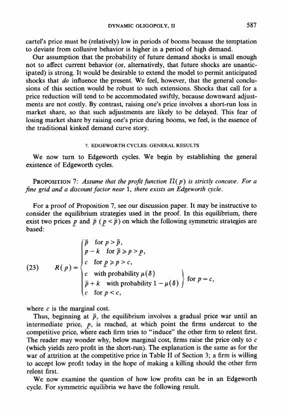
7. EDGEWORTH CYCLES: GENERAL RESULTS
We now turn to Edgeworth cycles. We begin by establishing the general existence of Edgeworth cycles.
PROPOSITION 7: Assume that the profit function 7f( p) is strictly concave. For a fine grid and a discount factor near 1, there exists an Edgeworth cycle.
For a proof of Proposition 7, see our discussion paper. It may be instructive to consider the equilibrium strategies used in the proof. In this equilibrium, there exist two prices p and p- (p <p) on which the following symmetric strategies are based:
p forp>p, p-k forp> p>p,
(23) R(p) = cfoppc c with probabilityu(8)6)
|p+ k with probability 1- u (8) ) P c c forp<c,
where c is the marginal cost. Thus, beginning at p, the equilibrium involves a gradual price war until an
intermediate price, p, is reached, at which point the firms undercut to the competitive price, where each firm tries to "induce" the other firm to relent first. The reader may wonder why, below marginal cost, firms raise the price only to c (which yields zero profit in the short-run). The explanation is the same as for the war of attrition at the competitive price in Table II of Section 3; a firm is willing to accept low profit today in the hope of making a killing should the other firm relent first.
We now examine the question of how low profits can be in an Edgeworth cycle. For symmetric equilibria we have the following result.
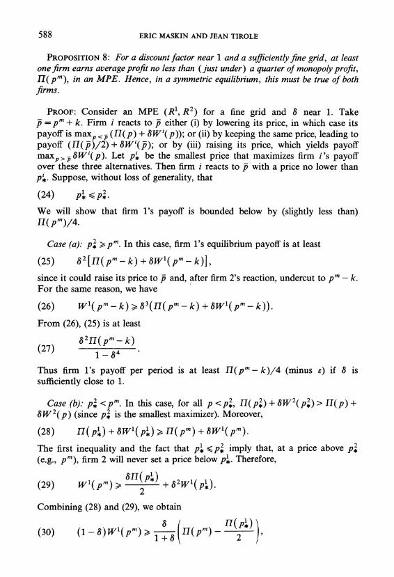
588 ERIC MASKIN AND JEAN TIROLE
PROPOSITION 8: For a discount factor near 1 and a sufficiently fine grid, at least one firm earns average profit no less than (just under) a quarter of monopoly profit, lI(ptm), in an MPE. Hence, in a symmetric equilibrium, this must be true of both firms.
PROOF: Consider an MPE (R', R2) for a fine grid and 8 near 1. Take p = ptm + k. Firm i reacts to p- either (i) by lowering its price, in which case its payoff is maxp <p (Ii(p) + 3W'(p)); or (ii) by keeping the same price, leading to payoff (H( -)/2) + 3W'(P); or by (iii) raising its price, which yields payoff maxp > W'(p). Let p* be the smallest price that maximizes firm i's payoff over these three alternatives. Then firm i reacts to p with a price no lower than p*. Suppose, without loss of generality, that
(24) 1 < p2
We will show that firm l's payoff is bounded below by (slightly less than) II(ptm)/4.
Case (a): p2 > pm. In this case, firm l's equilibrium payoff is at least
(25) s 2[Hw(p-mk) +3W1(pm-k)],
since it could raise its price to pi and, after firm 2's reaction, undercut to pm - k. For the same reason, we have
(26) Wl( pm -k) >, 83 (17(ptn- k) + SW'(pm -k)).
From (26), (25) is at least
2H82(pm - k)
Thus firm l's payoff per period is at least JI(pm - k)/4 (minus e) if 8 is sufficiently close to 1.
Case (b): p* < pm. In this case, for all p < p2, Hj(p2) + 6W2(p*2)> 11(p) +
SW2(p) (since p* is the smallest maximizer). Moreover,
(28) H(p,*) + 3W'(p ) > - H(pm) + (Wl(ppm).
The first inequality and the fact that pl <p2 imply that, at a price above p* (e.g., pm), firm 2 will never set a price below pD. Therefore,
(29) W(pm)> 2
Combining (28) and (29), we obtain
(30) (1- 8)Wl(pm)> H(ptM)>- ( I,) 1 +6 2 ,
DYNAMIC OLIGOPOLY, II 589
which implies that for 8 near 1,
(31) (1- O)Wl(pm) > I(p)
But (1 - S)Wl(pm) provides a lower bound for firm l's profit per period, since the firm has the option of setting pm. Hence II(pm)/4 also is a lower bound.
Q.E.D.
Thus regardless of the equilibrium, the average market price must be bounded away from the competitive price. We showed above that in a kinked demand curve equilibrium, aggregate profit per period must exceed four-sevenths of the Monopoly profit. This result and Proposition 8 show that one should not expect low prices in equilibrium if firms place enough weight on future profit. This conclusion contrasts with the properties of an MPE in the simultaneous-move price-setting game, where profits are very close or equal to zero (Bertrand equilibrium)."3
8. COMPARISON WITH THE QUANTITY MODEL
We have seen that our price model can give rise to a considerable multiplicity of equilibria: a range of kinked demand curve equilibria as well as Edgeworth cycles. By contrast, the model of capacity/quantity competition in our com- panion piece, although ostensibly very similar in structure, has a unique symmet- ric MPE.
The technical reason for this striking discrepancy is that the cross partial derivative of the instantaneous profit function fr behaves quite differently in the two models. In the quantity model, we assumed that (d 2sri)/( qdq'2) is negative -so that a firm's marginal profit is declining in the other firm's quantity. This implies that dynamic reaction functions are negatively sloped. The explanation for this negative slope is much the same as that for the downward sloping reaction functions in the static Cournot model: if marginal profit decreases as the other firm increases its quantity, then the quantity satisfying the first-order conditions for profit-maximization also decreases. (Were the cross partial always positive, reaction functions would be positively sloped.) Such nicely behaved reaction functions make the possibility of a multiplicity of symmetric equilibria a nonrobust pathology.
By contrast, the cross partial in our price model changes sign: when the other firm's price is sufficiently low (i.e., lower than its own price), a firm's marginal profit is zero; when the two prices are equal, marginal profit is negative (since
13 Assume that both firms are forced to play simultaneously (in odd periods, say). Then there is no payoff-relevant variable at the time firms make their decisions. Assume that the profit function is strictly concave in the firm's own price. If S2 is the mixed strategy of firm 2, firm l's profit can be written Sp Pr{ S2 = p } w&(pl, p). This function has a unique maximum or possibly two consecutive optitna p* and p* + k. The same holds for firm 2. A standard argument establishes that the maximum equilibrium price is c + k.
590 ERIC MASKIN AND JEAN TIROLE
raising one's price drives away all customers); finally, when the other firm's price is higher, a firm's marginal profit is positive if its price is below the monopoly level. This nonmonotonicity of marginal profit gives rise to dynamic reaction functions that are decidedly nonmonotonic. In the kinked demand curve de- scribed by (19)-(20), a firm will respond to a price cut above the relenting price p by lowering its own price. But below p a price cut induces it to raise its price to pf.
The price and quantity models also differ diametrically in their comparative statics. In the quantity model, an increase in the discount factor 8 means that firm 1 places greater weight on the future reduction of firm 2's quantity induced by a current increase in l's own quantity. Firm 1 therefore has the incentive to choose a correspondingly higher current quantity. Since the same reasoning also applies to firm 2, we conclude that an increase in 8 induces an increase in equilibrium quantities, i.e., a more competitive outcome. I
An increase in 8 in the price model, by contrast, makes it more worthwhile for a firm to sacrifice current clientele by raising its price today in the expectation of future profit when the other firm follows suit. Thus an increase in 8 may well detract from the competitiveness of the outcome. This is most clearly seen when we compare equilibrium for 8 = 0 (the only possible equilibrium price in the long run is very nearly marginal cost) with that for 8 near 1 (perfect collusion becomes possible).
Finally, the price and quantity models differ according to the value that length of commitment confers on a firm. We mentioned in the introduction to Part I of this study that contractual agreements may account for the sort of short-run commitment we have been discussing. The length of a contract, however, is in part a matter of choice, and so it is of some interest to consider the relative desirability of alternative conumitment periods. In the quantity model, it is clear that the incumbent firm is made better off as the length of its commitment grows. In the limit, it can attain monopoly profit by committing itself indefinitely. Thus, for contestability-like results to follow from a model where contracts form the basis of commitment, one must introduce some cost associated with lengthy contracts to prevent commitment of infinite duration.
In our price model, on the other hand, commitment serves as impediment to firms. To the extent that a firm is conumitted to a price, it will find it difficult to recapture lost market share should it be undercut. Thus, in this model, a firm will opt for contracts of the shortest possible length.
9. ENDOGENOUS TIMING
We now turn to the issue of alternating moves, and briefly examine how this timing might be derived rather than imposed. The first model is the discrete time framework with null actions described in Section 4 of Part I. Thus, a firm is free to set a price in any period where it is not already committed. Once it chooses a price, it remains committed for two periods. It also has the option of not setting a
DYNAMIC OLIGOPOLY, II 591
price at all, in which case it is out of the market for one period."4 Thus a Markov strategy for firm i takes the form { R1(.), S'}, where Ri(p) is, as before, i's reaction to the price p, and Si is its action when the other firm is not currently committed to a price.
We are interested in whether the alternating structure we imposed in Sections 2-8 emerges as equilibrium behavior in our expanded model. Accordingly, we will say that an MPE (Rl, R2) of the fixed-timing (alternating move) game is robust to endogenous timing if there exist strategies S' and S2 such that (i) ({ R', S1 }, { R2, S2 }) is an MPE of the endogenous, timing game; (ii) starting from the simultaneous mode, firms switch to the alternating mode in finite time with probability one. Notice that because R1 and R2 are equilibrium strategies of the fixed timing game, they never entail choice of the null strategy. Hence, once firms reach the alternating mode, they stay there forever.
Analogously, if (Sl, S2) is an MPE of the game in which firms are constrained to move simultaneously, we shall say that it is robust to endogenous timing if there exist reaction functions R' and R2 such that (iii) ({ R1, S1 }, { R2, S2 }) is an MPE of the endogenous-timing game; (iv) starting from the alternating mode, firms switch to the simultaneous mode in finite time with probability one. Our principal result of this section, proved in the Appendix, is the observation that symmetric alternating-move but not simultaneous-move MPE's are robust.
PROPOSITION 9: For a sufficiently fine grid and a discount factor near enough 1, any symmetric alternating-move MPE (R, R) but no simultaneous-move MPE (Sl, S2) is robust to endogenous timing.
The idea behind Proposition 9 is that, as we observed in footnote 13, firms earn very nearly zero profit in a simultaneous mode equilibrium, whereas, from Proposition 8, they earn at least a quarter of monopoly profit each in the alternating mode if 8 is near 1. Thus, in the simultaneous mode, a firm has the incentive to play the null action and move into the alternating mode. By the same token, neither firm has the incentive to upset alternating timing.
Of course, the endogenous-timing model of this section is only one of many possibilities. An even simpler, but perhaps less reasonable (for price competition), model that also leads to equilibrium alternation is a continuous time model with random (specifically, Poisson) commitment lengths."5 If every time a firm set a price, it remained committed to that price during the interval At with probability 1 - XAt, then the two periods of commitment in our discrete-time model
14 We thus assume that retailers, say, who do not receive a new price list, do not carry the firm's product. One alternative would be to assume that retailers continue to charge the old price. Gertner (1985) shows that the conclusions are robust to this specification. Another interesting aspect of Gertner's paper is that it allows menu costs of price changes exceeding the one-period monopoly profit (undercutting never pays in the short run, but reactions to price cuts are also very costly). This reflects the possibility that decision periods are very short.
15 For a fuller description of this example see our companion paper.
592 ERIC MASKIN AND JEAN TIROLE
correspond exactly to the mean commitment length in the stochastic model. Moreover, all our results for the former model go through for the latter.
10. COMPARISON WITH SUPERGAMES
Several of the results of this paper underscore the relatively high profits that firms can earn when the discount factor is near 1. Thus our model can be viewed as a theory of tacit collusion. There is, of course, a variety of other such theories. The literature on incomplete information in dynamic games, for example, has shown that high prices may be sustained by oligopolists' desire to mislead their rivals. Kreps-Milgrom-Roberts-Wilson (1982) demonstrate the advantages of cultivating a reputation for being intrinsically cooperative. The firms in (the price interpretation of) Riordan (1985) secretly charge high prices today to signal to their competitors that demand is high, so as to induce them to charge high prices tomorrow.
Another (more closely-related) alternative is the well-established supergame approach to oligopoly. Starting with Friedman (1977), the theory has produced many interesting applications, among them Brock-Scheinkman (1985), Green- Porter (1984), and Rotemberg-Saloner (1986), and undergone several develop- ments, e.g., Anderson (1984) and Kalai-Stanford (1985). W-e feel, however, that our approach may offer certain advantages over the supergame line. nature. A firm conditions its behavior on past prices only because other firms do so. If we eliminate the bootstrap equilibria, we are left with lack of collusion. Moreover, the strategies in the supergame literature typically have a firm reacting not only to other firms but to what it did itself.'6 By contrast, a Markov strategy has a firm condition its action only on those variables that are relevant in all cases of other firms' behavior. Thus, in a price war, a firm cuts its price not to punish its competitor (which would involve keeping track of its own past behavior as well as that of the competitor) but simply to regain market share. It strikes us that these straightforward Markov reactions often resemble the infor- mal concept of reaction stressed in the traditional industrial organization discus- sion of business behavior (e.g., the kinked demand curve story) more closely than do their supergame counterparts.
Second, supergame equilibria rely on an infinity of repetitions. They break down even for long but finite horizons.'7 For example, any finite number of repetitions of the Bertrand price-setting game yields the competitive price at every iteration."8 We have not yet been able to prove that equilibrium in the finite period version of our price model converges to the infinite period equi-
16 Indeed, this "self-reactive" property is often essential to obtaining collusion (see Section 3B of Maskin-Tirole (1982)).
17 Unless there are multiple equilibria in the constituent game (see Benoit-Krishna (1985)). 18 One can preserve supergame equilibria by replacing the infinite horizon with a reasonably high
probability in each round that the game will continue another period. But this extension does not cover the case where the horizon length is determined fairly well in advance.
DYNAMIC OLIGOPOLY, II 593
librium as the horizon lengthens.'9 But we have at least shown that for a long enough finite horizon, equilibriSum is not "close" to the competitive equilibrium, a result similar to Propositions 3 and 8.
Third, the supergame approach is plagued by an enormous number of equi- libria. In the repeated Bertrand price game, any feasible pair of nonnegative profit levels can arise in equilibrium with sufficiently little discounting. Our model too has a multiplicity of equilibria but a smaller one. Propositions 3 and 7 demonstrate, for example, that profits must be bounded away from zero. More- over, from Proposition 5, there is only a single equilibrium20 that sustains monopoly profits (whereas there is a continuum of such equilibria in the supergame framework).
Finally, the supergame approach makes little distinction between price and quantity games: in either case any profit level between pure competition and pure monopoly is achievable for 8 near 1. As we suggested in Section 9, however, our approach does distinguish between the two. Quantity/capacity games are marked by downward sloping reactions functions and an increase in competition as the number of interactions between firms increases (or the future becomes more important), whereas price games exhibit nonmonotonic reaction functions and a decrease in competition as 8 rises. (In the terminology of Bulow et al. (1985), quantities are strategic substitutes, while prices are strategic complements for a range of prices and strategic substitutes for another.)
11. EXCESS CAPACITY AND MARKET SHARING
Although important, price is only one dimension in which oligopolists com- pete. In particular firms also make quantity decisions. In Maskin-Tirole (1985), we provide two simple examples that show how our model can be extended to provide explanations of excess capacity and market sharing.
Excess Capacity
In the kinked demand curve equilibrium of Example 1, undercutting the monopoly price is deterred by the threat of a price war. Recall, however, that in this example firms are not capacity constrained. Once we introduce such con- straints, it is easy to see that the monopoly price may not be sustainable if firm 2 has only enough capacity to supply half the demand at the monopoly price. Indeed, firm 1 will wish to undercut if it has more than this capacity, and firm 2 will not be able to respond effectively because it cannot expand output at lower prices to reduce the first firm's market share. Thus the threat of a price war is a significant deterrent to price cutting only if firms have more capacity than they will use when price is at the monopoly level.
19 We have, however, obtained just such a convergence result for the Cournot competition version of the model (Maskin-Tirole (1987)).
20 This equilibrium is, in fact, renegotiation-proof.
594 ERIC MASKIN AND JEAN TIROLE
In the extended model of Maskin-Tirole (1985), firms choose capacities simultaneously and once-and-for-all; they then compete through prices as in Section 3. We exhibit an MPE in which firms accumulate capacities above the level necessary to supply half the market at the monopoly price, and yet charge the monopoly price forever. That is, the firms accumulate capacities that they never use simply to make undercutting less attractive for their rivals.
Market Sharing
In a static model, a firm always supplies the demand it faces as long as price exceeds its marginal cost. In a dynamic framework, however, a firm may temper its rival's aggressiveness by voluntarily giving up some of its market share. In Maskin-Tirole (1985), we construct an example in which firm 1 has a marginal cost lower than that of firm 2. When a firm chooses a price, it also chooses a selling constraint, i.e., the maximum quantity that it can supply at its chosen price (corresponding, for example, to the extent of its inventory). In the MPE, the firms charge a price above the monopoly price of firm 1 but below that of firm 2. To avoid triggering price-cutting by the low-cost firm, firm 2 imposes a market share less than one-half on itself. It thus "bribes" firm 1 to accept a compara- tively high market price.21
Department of Economics, Harvard University, Cambridge, MA 02138, U.S.A. and
Department of Economics, MIT, Cambridge, MA 02139, U.S.A.
Manuscript received June, 1985; final revision received July, 1987.
APPENDIX
PROOF OF PROPOSITION 4: We must show that any price in [x, y] is a focal price for sufficiently high discount factors. To do this, we will consider three cases depending on the relative magnitudes of n(pf) and (2/3)II(pm) and of pf and pm, where pf is the focal price candidate in lx, y]. In each case, we will exhibit the equilibrium strategies giving rise to p1.
Case (a): H(pf) > (2/3)l(pm) and pf <pm. In this case, equilibrium consists of both players using the strategy
(pf, forpaptf,
R (p) = p, forpf >p >p,
pf, forp p,
where p is chosen so that
4II(p) > H(pm) > 4H(p - k)
(notice that the existence of p is ensured by a sufficiently fine price grid).
21 This is an example of a "puppy-dog" strategy: remain small so as not to trigger aggressive behavior by one's rival (see Fudenberg-Tirole (1984)).
DYNAMIC OLIGOPOLY, II 595
Case (b): H(pf)> (2/3)H(pm) and pf>pm, In this case the equilibrium strategy for each player is
{p,forp>-Pf
Pl, forpf>p>pi,
R Pl, with probability a l
p, with probability 1-a J
p , for p1 >p >p,
pf, forp p,
where pf > pm > p, >p and
H(p)(l +8)>8 8N2 > , I(p k)(1 +8),
(82 + 83 H (pi) f H(p1) ~82 +83 H(-p)(1+?)+a 2 H(p)2 (2 ?alj 2 2
H(pi) =H(pf) -,
for - small.
Case (c): H(pf) < (2/3)I(p') and pm >pf > x. Now we take
p, if p >p, | , with probability a
pf, with probability 1-a )f P p, R( p) = pf, ifp>p?,Pf,
p, if pf>p>p,
p, ifp p,
where p"'>p>pf>p and
n(p) (pf)(I+ 8 >(p(P-)k),
2
v(P) () + 8w(P) = n(pf) + 8 H(P f),
HI(p)(l + 8) + 82V(p) > 8W(P) > H(p - k)(I + 8) + 82 V( p),
(2 + 8)I(pf) - H(p) 6H
(j))+82H(pf)
Here V(p) is the valuation of a firm when its rival has just played p, and W(p) is the firm's valuation when it itself has just played p. Notice that p5 as defined above exists and is unique, since 11(pf) < (2/3)I1(pm). For 8 large and k small, a is approximately equal to one fifth.
For the straightforward verification that the strategies defined in Cases (a)-(c) form equilibria, see Maskin-Tirole (1985). Q. E. D.
PROOF OF PROPOSITION 5: Fix the price grid. Assume for convenience that:
(AO) there exists no feasible price p such that 11(p) = H( p' )/2.
For any a E (0, 1), there exist e > 0 and 8 < 1 such that, if (RI, R2) is an MPE (with discount factor
596 ERIC MASKIN AND JEAN TIROLE
8> 8) such that
(Al) (l-8)(Vl(p)+ W2(p))> H(pn)- E for some p,
then
(A2) Prob { R'(p')>pm}> a for i=1,2.
If E is small and 8 is near 1, then (Al) implies that the market price is pm most of the time. But then the reaction to pm must, with high probability, be a price p no less than pm (if p <pm, then p becomes the market price).
Formula (A2) ensures that, for a near 1, a firm can guarantee itself a payoff of nearly H(pm)/2 per period simply by always setting the price pm. Indeed, if Prob { R'(p') > pt } is near 1, firm j can obtain nearly H(pt) per period from this strategy. Hence, for E small and 8 near 1, an MPE (Rl, R2) satisfying (Al) also satisfies
(A3) II(p')12- V'(pn)(1 -8)> II(p)12, for all p Opm, and
(A4) Prob {RI(pm)=pm}>O, i= 1,2
Formula (A4) implies that p mis a semi-focal price. We first claim that if (R, R2) satisfies (Al) for E small and 8 near 1, then
(A5) p>pm implies R'( p) =pm for i = 1,2.
Let p be in the support of Ri( p) for some i and p >pm. Because ptm is a semi-focal price,
(A6) pE[pm p]
Suppose that p is the smallest price such that p E (ptm, p] for some realization p of Ri( p). If p <p, then
(A7) Vi(P)= H(p)+82Vi(pm)
which contradicts the facts that V1(p) > V(ptm) and Vl(ptm)(l - 8) H Il(ptm)/2 for 8 close to 1. If p=p, then
VI(p) < (l/2)H(p)(l + 8) + 82Vi
since RJ(p) < p and Vi(.) is nondecreasing. Hence V1(p)(1 - 8) < II(p)/2, which again contradicts (A3). We conclude that (A5) holds after all.
We next argue that, for the MPE under consideration,
(A8) if p < pm and p is a realization of R' (p), then p ptm.
If instead p > pm, then from (A5)
(A9) 82V1(pm)?8Wi(pni).
But from (A4),
(AlO) VI (pm) =H(ptm)/2+8W (ptm).
Formulas (A9) and (AlO) imply that
H(ptm) WI (PM)(' -8) <8 '(PM8)
which contradicts (A3) and (AlO). Hence, (A8) holds. Next we demonstrate that
(All) if p <-pm and p ( > p) is a reahzation of R'(p), then p =pn.
Clearly, if p is a realization of R1( p) and p > p, we have
(A12) WI(p) ? WI(ptM).
DYNAMIC OLIGOPOLY, II 597
From (A8) p 6 pt, and so, if p * pm,
(A13) II (p)/2 + 8 W1(p) > H(p) + ?8W(p).
Thus (AO), (A12), and (A13) imply that
(A14) '(PM)
> I(P)- 2
Now, RJ(p) 6 pm. Hence, because V'(-) is nondecreasing and pm is a realization of R'(pm),
(A15) W(p)6 ,(p) + 8v(PM) = n(p) + 8 (P ) +82W(pm). 2
From (A12) and (A15) we infer
W1(PM)(1l8)< (n(P)+8 '(PM) (1 + 8),
which, in view of (A14), contradicts (A3) and (A10). Hence (All) holds. We next argue that
(A16) forallp6p, R'(p)=pm, i=1,2,
where p is defined by (20). For i = 1, 2, define pi so that
82Hl(pm)+8 i(m (A17) (1 +8)H(p) + 2 +8W(p)
82HI(M) 8w(pm) . > 8W1(pm)> (1 + 8)H(p' - k) + 2 + +3W(pm).
Rearranging, we obtain
(A18) (1-+8)H(pl -k) + 82 (pm) <8(l+ 8)W (pM)(l-8)
<(1 + 8)H (pl) + 82H(PM) 2
Now, for 8 near 1, the middle expression of (A18) is nearly IH(pm). Hence, for such 8, p1 =p, i = 1, 2. Consider firm i when the current market price p is less than or equal to p. If it chooses a price no higher than p, then an upper bound on its payoff is the right side expression-of (A17), since the best it can hope for is that the other firm reacts by raising its price to pm. If, instead, firm i raises its price to p", it obtains the middle expression of (A17). The second inequality of (A17), therefore, establishes (A16).
We must now show that
(A19) forpe(p,pm) Rl(p)=p, i=1,2.
Consider p E (p, p"). From the first inequality in (A17), a firm is better off cutting its price to p than raising it to p"7 when the current price is p. The only other possibility is that the firm could choose some price in (p, p]. Let p be the smallest price in (p, ptm] for which for some firm i there exists p (p, p] in the support of RI( p). Then, from (A16),
(A20) V (p< I(p)+83 W (pm).
If, however, firm i raises its price directly to pm from p, it obtains 8W(p`'), which (since (1 - 8) Wl(pm) is nearly HI(pm)/2) is greater than the right side of (A20), a contradiction. We conclude that (A19) holds after all.
We have demonstrated that for E small and 8 near 1, an MPE (R1, R2) satisfying (Al) also satisfies (19) for p #pn'. It remains to show that Rl(pm) =pn'. Let p be a realization of Rl(p"'). If p > pn, then (A5) implies that Vi(pm') =82Vi(pm), which is clearly false. The argument of the previous paragraph ((A20) in particular) demonstrates that p cannot lie in (p, pn'). Suppose p = p.
598 ERIC MASKIN AND JEAN TIROLE
Then V(pm) = II(p)(l + 8) + 82V(p,), which implies (1 - 8)V(p') = H(p), a contradiction of the fact that (1 - 8)V(7pm) is near H(pm)/2. Thus, we conclude that R(pm) =pm. Q.E.D.
PROOF OF PROPOSITION 9: Consider a symmetric MPE (R, R) of the alternating-move model, and let V(p) and W(p) be the associated valuation functions. Let p denote the smallest price that maximizes Il(p) +8 W(p). We will construct a strategy S* for the simultaneous mode such that ( R,S*)) forms an MPE for the endogeneous-timing game.
For the moment, suppose that firms, when in the simultaneous mode, can choose either (a) the null action or (b) a price no greater than p (we will admit the possibility of firms' choosing prices greater than p later on). Once we specify firms' behavior in this mode, then their payoffs are completely determined, assuming they play according to R in the alternating mode. Thus we can think of firms in the simultaneous mode as playing a one-shot game in which they choose mixed strategies S1 and S2 and their payoffs are determined by ({ R, Sl }, (R, S2)). Because this is a symmetric game there exists a symmetric equilibrium (S*, S*). Let U* be a firm's corresponding present discounted profit. We claim that ({ R, S*), { R, S*}) is an MPE for the endogenous-timing game.
We first note that S* must place positive probability on the null action. If this were not the case, then firms would remain in the simultaneous mode forever. But, as we argued in footnote 13, any simultaneous-mode equilibrium must entail (essentially) zero profit. By contrast, if a firm played the null action and thereby moved the firms into the alternating mode, Proposition 8 would guarantee it at least a quarter of monopoly profit, which is clearly preferable. Thus SF must indeed assign the null action positive probability.
We next observe that, in the simultaneous mode, firm i cannot gain from choosing a price p greater than p, given that firm ] sticks to S*. If firm j does not choose the null action-i.e., it selects a price-then firm i sells nothing with a price greater than p. If firm j does select the null action, then the firms move into the alternating mode, and firm i's payoff is H(p) +8 W(p), which, by definition of p, is no greater than that from choosing p. Hence a firm has no incentive to choose prices greater than p in the simultaneous mode.
It remains only to show that, in the alternating mode, a firm has no incentive to play the null action. If it did so, its payoff would be 8U*, since the firm would then be in the simultaneous mode. Now, because, as we have noted, it is optimal for a firm to play the null action in the simultaneous mode,
U* < 8V(p).
Hence, by playing the null action in the alternating mode, a firm obtains a payoff less than 82V(p). If instead it chooses a price p > p, the other firm will react with a price no lower than p, and so its payoff is at least 82 V(p). Hence the null action is not preferable.
To see that a simultaneous-move MPE (S1, s2) cannot be robust to endogenous timing, recall that in such an equilibrium, S' ? c + k for i =1, 2. Now if (S', S2) were robust, there would exist reaction functions R' and R2 such that, starting from the alternating mode, firms switch to the simultaneous mode in finite time and remain there forever. But, using much the same argument as in the proof of Proposition 8, we can show that at least one firm can obtain a per period equilibrium payoff that is bounded well away from zero, which contradicts the upper bound of H(c + k)/2 it earns in the simultaneous mode. Q.E.D.
REFERENCES
ABREU, D. (1986): "Extremal Equilibria of Oligopolistic Supergames," Journal of Economic Theory, 39,191-225.
ANDERSON, R. (1984): "Quick Response Equilbrium," IP323, Center for Research in Management, University of California-Berkeley.
BENOIT, J. F., AND V. KRiSHNA (1985): "Finitely Repeated Games," Econometrica, 53, 890-904. BERTRAND, J. (188$): "Review of 'Theorie Mathematique de la Richesse Sociale et Recherches sur les
Principes Mathematiques de la Richesse'," Journal des Savants, 499-508. BROCK, W., AND J. SCHEINKMAN (1985): "Price Setting Supergames with Capacity Constraints,"
Review of Economic Studies, 52, 371-382. BULOW, J., J. GEANAKOPLOS, AND P. KLEMPERER (1985): "Multimarket Oligopoly: Strategic Sub-
stitutes and Complements," Journal of Political Economy, 93, 488-511. DERMAN, C. (1970): Finite State Markovian Decision Processes. New York: Academic Press.
DYNAMIC OLIGOPOLY, II 599
EDGEWORTH, F. (1925): "The Pure Theory of Monopoly," in Papers Relating to Political Economy, Vol. 1. London: MacMillan, pp. 111-142.
FARRELL, J., AND E. MASKIN (1987): "Renegotiation in Repeated Games," mimeo, Harvard Univer- sity.
FRIEDMAN, J. (1977): Oligopoly and the Theory of Games. Amsterdam: North-Holland. FUDENBERG, D., AND J. TIROLE (1984): "The Fat-Cat Effect, the Puppy-Dog Ploy, and the Lean and
Hungry Look," American Economic Review, 74, 361-366. FUDENBERG, D., AND E. MASKIN (1986): "The Folk Theorem in Repeated Games with Discounting
or with Incomplete Information," Econometrica, 54, 533-554. GERTNER, R. (1985): "Dynamic Duopoly with Price Inertia," mimeo, MIT. GREEN, E., AND R. PORTER (1984): "Noncooperative Collusion under Imperfect Price Information,"
Econometrica, 52, 87-100. HALL, R., AND C. HITCH (1939): "Price Theory and Business Behavior," Oxford Economic Papers, 2,
12-45. KALAI, E., AND W. STANFORD (1985): "Conjectural Variations Strategies in Accelerated Coumot
Games," International Journal of Industrial Organization, 3, 133-152. KREPs, D., P. MILGROM, J. ROBERTS, AND R. WILSON (1982): "Rational Cooperation in the
Finitely-Repeated Prisoner's Dilemma," Journal of Economic Theory, 27, 245-252. MASKIN, E., AND J. TiRoLE (1982): "A Theory of Dynamic Oligopoly, I: Overview and Quantity
Competition with Large Fixed Costs," MIT Working Paper #320. (1985): A Theory of Dynamic Oligopoly, Part II: Price Competition," MIT Working Paper
373. (1987): "A Theory of Dynamic Oligopoly, Part III: Coumot Competition," European
Economic Review, 31, 947-968. (1988): "A Theory of Dynamic Oligopoly, Part I: Overview and Quantity Competition with
Large Fixed Costs," Econometrica, 56, 549-569. - RIORDAN, M. (1985): "Imperfect Information and Dynamic Conjectural Variations," Rand Journal of
Economics, 16, 41-50. ROTEMBERG, J., AND G. SALONER (1986): "A Supergame-Theoretic Model of Business Cycles and
Price Wars During Booms," American Economic Review, 76, 390-407. RUBINSTEIN, A. (1980): "Strong Perfect Equilibrium in Supergames," International Journal of Game
Theory, 9, 1-12. SCHERER, F. (1980): Industrial Market Structure and Economic Performance, Second Edition. Rand
McNally. SWEEZY, P. (1939): "Demand Under Conditions of Oligopoly," Journal of Political Economy, 47,
568-573.