A tale of two laws -...

Article

The International Journal of HighPerformance Computing Applications2015, Vol. 29(3) 320–330� The Author(s) 2015Reprints and permissions:sagepub.co.uk/journalsPermissions.navDOI: 10.1177/1094342015572031hpc.sagepub.com

A tale of two laws

Michael T Heath

AbstractAs Amdahl’s law and Moore’s law reach their 50th anniversaries, we review the roles they have played in shaping bothperception and reality in high-performance computing. Along the way, we also attempt to clarify some misconceptionsthat have surrounded both of these highly influential but not always fully appreciated ‘‘laws.’’

KeywordsAmdahl’s law, Moore’s law, parallel computing, scalability, speedup, efficiency, Dennard scaling

1. Amdahl, Moore, and you

Amdahl’s law and Moore’s law have had a profoundimpact on the evolution of high-performance comput-ing (HPC). The two laws are of similar vintage, bothhaving been formulated in the mid-1960s at the dawnof the modern era of HPC, but they differ markedly inmany other respects. Amdahl’s law expresses a mathe-matical relationship whose conclusion is logically unas-sailable, but the applicability of its hypotheses has beenthe subject of considerable debate. Moore’s law, on theother hand, expresses an empirical observation abouttrends in technological capability and manufacturingefficiency, but its extraordinary predictive accuracy hasdepended to a large extent on self-fulfilling prophecy.Amdahl’s law provoked widespread skepticism con-cerning the ultimate potential of parallel computing,whereas Moore’s law engendered great optimism forthe future of computing in general and eventuallyenabled the present ubiquity of computers in daily life.Accordingly, heroic efforts have been expended both tocircumvent Amdahl’s law and to prolong Moore’s law.As they reach their 50th anniversaries, we review theroles played by these two highly influential ‘‘laws’’ inshaping both perception and reality in HPC. We exam-ine how and why each law came to be formulated, howpractitioners have grappled with their implications inthe intervening years, and why both remain relevanttoday.

2. Parallel scalability

Serious interest in parallel computing dates from themid-1960s, with ILLIAC IV (designed 1965–66, deliv-ered 1971) often cited as the first ‘‘massively’’ parallel

computer, designed to have 256 processing elements(although only 64 were actually fabricated) (Hord,1982). By this time transistors had replaced the vacuumtubes and relays in the logic circuits of the first genera-tion of electronic digital computers, but integrated cir-cuits (invented in 1958) were still in their infancy, socomputers were made of individually wired compo-nents that filled large cabinets or whole rooms. Butimprovements in the speed of such ‘‘macro’’ computerswere beginning to level off, due to physical constraintssuch as the speed-of-light limit (about one foot pernanosecond) on signal propagation, thus the growinginterest in applying many processors in concert to solvea single problem.

The primary motivation for parallel computing is toincrease computational speed (work per unit time) byspreading the work over more processors. The goalmight be:

� to solve a given problem (same work) in less time;� to solve a larger problem (more work) in the same

time; or� to gain sufficient capacity to solve ever larger prob-

lems regardless of time.

Department of Computer Science, University of Illinois at Urbana-

Champaign, Urbana, IL, USA

Corresponding author:

Michael T Heath, Department of Computer Science, University of Illinois

at Urbana-Champaign, 201 North Goodwin Avenue, Urbana IL 61801,

USA.

Email: [email protected]

Qualitatively, scalability refers to the relative effective-ness with which additional processors can be used: asthe number of processors increases, does performanceincrease commensurately? As we will see, however, thisconcept is not easy to quantify, and often difficult toachieve. To help quantify scalability, the followingquantities are conventionally defined for a givenproblem:

� processors, p = number of processors used;� execution time, T(p) = elapsed wall-clock time

using p processors;� cost, C(p) = pT(p), measured in processor-seconds,

processor-hours, etc.;� speedup, S(p) = T(1)/T(p);� efficiency, E(p) = C(1)/C(p) =

T(1)/(pT(p)) = S(p)/p.

The goal then becomes to solve the problem p times asfast, S(p) = p, by using p processors, which is equiva-lent to achieving 100% efficiency, E(p) = 1. In prac-tice, such ideal performance is unattainable (barringeffects of cache or chance), and one settles for somelower level of efficiency E(p) \ 1. Arbitrarily low effi-ciency is obviously unacceptable, however, so a mini-mal criterion for scalability is that E(p) be boundedaway from zero as p!N. As we will see, however, eventhis seemingly innocuous criterion can be difficult orimpossible to meet in many practical situations.

2.1 Empirical speedup considered harmful

Note that speedup and efficiency depend on the serialtime T(1), but what does T(1) really mean? Plausibleanswers include:

� execution time for the parallel code using oneprocessor;

� execution time for the corresponding serial codeusing one processor (i.e. the same basic algorithmbut without any parallel overhead); or

� execution time for the ‘‘best’’ serial algorithm;

but none of these is truly satisfactory. Running the par-allel code on a single processor generally incurs signifi-cant overhead for communication and synchronizationthat is unnecessary when p = 1. Even if this paralleloverhead is removed or bypassed in a serial version ofthe code, the underlying parallel algorithm may not beoptimal when p = 1. The criterion for ‘‘best’’ serialalgorithm may not be clear-cut (least computing time,least memory usage, etc.), and the optimal choice maydepend on particular problem features, such as prob-lem size. Moreover, using a fundamentally differentalgorithm for the special case p = 1 introduces a

disruptive discontinuity that resets the particular levelof efficiency but usually does not alter the overall trendin relative performance as p varies.

Further complicating matters, the problem of inter-est may not fit in the memory of a single processor,making direct measurement of T(1) impossible. Onealternative approach is to use the smallest p for whichthe problem fits in memory as a benchmark for com-puting relative speedup, but this particular choice seemsarbitrary, and in any case cache behavior may differgreatly as p varies, yielding erratic computed speedupsthat are not very meaningful.

But who cares about serial execution time anyway?Today’s users are not interested in what happens whenthey go from 1 processor to 100,000 processors, theyare interested in what happens when they go from100,000 processors to 200,000 processors. Thus, theycare about the behavior of their parallel code, not thatof some mythical serial code. We conclude that becauseof their dependence on often ill-defined or irrelevantserial execution time, speedup and efficiency as conven-tionally defined are often not useful measures of paral-lel performance for real programs.

2.2 A better alternative

Rather than using a derived measure such as speedup toassess scalability, a better alternative is simply to plotraw execution data, specifically a log–log plot of T(p)versus p, for a systematic sequence of runs, varying thenumber of processors (Van de Velde, 1994). Two com-mon instances of this approach are:

� Strong scaling: for a fixed problem, a straight linewith slope 21 indicates good scalability, whereasany upward curvature away from that line indicateslimited scalability.

� Weak scaling: for a sequence of problems with afixed amount of work per processor, a horizontalstraight line indicates good scalability, whereas anyupward trend of that line indicates limitedscalability.

An example of strong scaling is shown in Figure 1,where the bullets represent execution times for a fixedproblem using various numbers of processors (datagenerated synthetically). The solid line is a least-squaresfit of a straight line with slope 21 to the given datapoints (plotting such a line is not strictly necessary, butit can be a helpful visual aid). Note that the smallestnumber of processors for which the problem fits inmemory happens to be 16, but no notion of relativespeedup is required. The tailing off in scalability is evi-dent for p . 104.

Heath 321

3. Amdahl’s law

The foregoing observations were aimed at empiricalperformance analysis for real parallel programs.Theoretical performance models can often providevaluable insight into the scalability of the underlyingparallel algorithms independent of any specific imple-mentation. By assuming away memory limitations,cache effects, etc., the conventional definitions of con-cepts such as speedup and efficiency can be appliedmeaningfully and unambiguously in this theoreticalcontext. One of the earliest and easily the most famoussuch theoretical performance model forms the basis forAmdahl’s law. Amdahl’s original paper (Amdahl, 1967)provided only a verbal description of the relationshipthat later became known as Amdahl’s law, but it isequivalent to the following mathematical statement.

Amdahl’s law. If a fraction s of the work for a givenproblem is serial, with 0 \ s � 1, while the remainingportion, 1 2 s, is p-fold parallel, then

T (p)= sT(1)+ (1� s)T (1)

p

S(p)=T (1)

T (p)=

1

s+(1� s)=p

E(p)=T (1)

pT(p)=

1

sp+(1� s)

and hence S(p)! 1/s and E(p)! 0 as p!N.If the serial fraction s exceeds 1%, for example, thenthe speedup can never exceed 100 no matter how manyprocessors are used, and the efficiency becomes arbitra-rily low as increasingly many processors are used.

Amdahl’s pessimistic conclusion of limited speedupand poor efficiency should come as no surprise, at leastqualitatively, as no fixed, finite amount of work can beshared profitably by arbitrarily many processors, with

the obvious negative ultimate consequences for speedupand efficiency. Nevertheless, Amdahl’s quantifying ofthese effects, albeit in the context of a very simple com-putational model, served as an eye opener that justifieda continued emphasis on further improving serial com-puting speeds (aided largely by Moore’s law, as we willsee), as well as extensive efforts to circumvent Amdahl’sunwelcome strictures.

Since Amdahl’s simple derivation is valid mathema-tically, to avoid his sobering conclusion one must evadehis hypotheses. One could argue, for example, that theassumed dichotomy between serial and p-fold parallelportions is too simplistic. But in fact it is not an unrea-sonable proxy for the inevitable lack of perfect paralle-lism in most computational problems due to precedenceconstraints, communication overhead, etc. To illustrate,consider these typical examples of parallel performancemodels for some common numerical computations,where nmeasures problem size in basic work units:

� summation of n numbers, T(p) ’ n/p + log p;� solution of a triangular system of order n, T(p)

’ n2/p + n;� LU factorization of a matrix of order n, T(p) ’ n3/p+ n;� solution of a tridiagonal system of order n, T(p)

’ (n log n)/p + log p.

These examples were chosen to represent a number ofrealistic situations that arise often in practice.Summation is ubiquitous, of course, but a similar com-plexity model, having a perfectly parallel phase fol-lowed by a reduction whose length grows at leastlogarithmically with p, applies to many other computa-tions, such as computing inner products, convergencetests for iterative methods, and Monte Carlo simula-tions in which independent trials are computed simulta-neously in parallel and then all of the results must beaveraged to produce the final result. Solution of trian-gular linear systems and LU factorization with an n 3

n matrix typify many problems for which the bulk ofthe computation is highly parallel, but due to prece-dence constraints there is a serial thread (here of lengthn) running through the computation, the length ofwhich grows with problem size. Solution of tridiagonalsystems incurs additional work in order to introduceparallelism into an otherwise inherently sequentialcomputation.

Log–log performance plots for these examples (nor-malized by the total amount of work in each case) areshown in Figure 2, along with performance plots givenby Amdahl’s law for various serial fractions s. Thebehavior and scalability of the real examples is visuallyindistinguishable from those for Amdahl’s law with anappropriately chosen serial fraction s. In each case, theserial fraction is an effective proxy for the terms in the

Figure 1. Log–log performance plot.

322 The International Journal of High Performance Computing Applications 29(3)

performance model that do not decrease as p increases.In fact, for any parallel computation one can infer aneffective serial fraction empirically from measuredspeedup, as in the Karp–Flatt metric (Karp and Flatt,1990), although empirical speedup has its own short-comings, as we have already seen. Thus, one cannotdeny the applicability of Amdahl’s law simply by argu-ing that the performance model underlying it is toounrealistic, and therefore one must grapple with the(effective) serial fraction for a given problem of interest.

3.1 Consequences of Amdahl’s law

Fortunately, for most problems the effective serial frac-tion decreases as problem size increases, and henceAmdahl’s limits on speedup and efficiency become cor-respondingly less onerous. Thus, the most commonresponse to the limited speedups and declining effi-ciency implied by Amdahl’s law is to solve increasinglylarger problems as the number of processors increases(Gustafson, 1988; Singh et al., 1993). However, the rateof growth in problem size, relative to the growing num-ber of processors, is constrained: if the problem sizegrows too slowly, then efficiency may decline unaccep-tably, but if the problem size grows too rapidly, thenexecution time may grow unacceptably. Thus, solvingever larger problems is not a panacea, but a two-edgedsword that necessitates walking a fine line betweendeclining efficiency and growing execution time, whichmay not be possible in practice, as we will see next.

Amdahl’s key observation was that any inherentlyserial work imposes a lower bound on execution timethat is independent of the number of processors.Increasing the problem size can reduce the proportionof serial work, but it often increases the total amount ofeffectively serial work, and thus the lower bound onexecution time increases with problem size. Increasingproblem size also increases the parallel portion of the

execution time unless the problem size grows no fasterthan the number of processors. Thus, total executiontime increases unless the problem size grows moreslowly than the number of processors, yielding declin-ing efficiency.

One can infer from Amdahl’s law how rapidly theserial fraction must decrease with increasing problemsize in order to achieve a desired efficiency. For exam-ple, to maintain a given constant efficiency E,0 \ E � 1, Amdahl’s law requires that

s=1� E

E� 1

p� 1

Applying this result to a performance model of interestthen determines the corresponding minimum growthrate in problem size. For example, if T(p) ’ n/p + logp, then the problem size n must grow proportionally top log p, causing execution time to grow like log p. Moregenerally, this observation leads to one of the most use-ful measures of scalability, the isoefficiency function,which is defined to be the minimum rate at which theproblem size (as measured by the total amount of com-putational work) must grow in order to maintain con-stant efficiency as p grows (Grama et al., 1993). Thegrowth rate of the isoefficiency function with respect tothe number of processors then characterizes the degreeof scalability:

� Y(p), highly scalable;� Y(p log p), reasonably scalable;� Y(p

ffiffiffi

pp

), moderately scalable;� Y(p2) or higher, not scalable.

For a given problem, its isoefficiency function dividedby p gives the growth rate of the execution time as pincreases. For example, if the isoefficiency function isY(p2), then doubling the number of processors alsodoubles the execution time, which is clearly untenable.For any slower growth rate, however, constant effi-ciency cannot be maintained, and efficiency necessarilydeclines.

We have just seen that except for the usually unat-tainable ideal isoefficiency function Y(p), executiontime necessarily increases, and possibly quite rapidly,unless one is willing to accept ever lower efficiency.Incurring ever longer turnaround times in order to meetefficiency goals may or may not be acceptable, depend-ing on the purpose of the computation. Turnaroundtime may be limited by, among other factors:

� hard real-time constraints, as in control systems orweather prediction;

� practical working schedules requiring say hourly ordaily turnaround;

� mean time between failures of computingequipment.

Figure 2. Scalability of various performance models.

Heath 323

Even when limiting turnaround time is not crucial,there may still be little or no value in solving ever largerproblems. For example, over-resolving a problembeyond the accuracy needed or beyond that warrantedby the available data solely to achieve higher parallelefficiency is of dubious value.

For example, if you are trying to intercept an incom-ing missile, then it is not helpful to assume 10 or 100incoming missiles instead, because you will not be aroundto brag about the improved efficiency with which youcan track them. For weather prediction, efficiency couldbe improved through increasing problem size by:

� refining the spatial resolution of the computationalmesh;

� enlarging the geographic region covered; or� adding more detailed physics;

but none of these will decrease turnaround time andare instead likely to increase it, eventually threateningthe ability to make timely predictions. Additional pro-cessors can potentially be used more helpfully to per-form sensitivity analysis or uncertainty quantification,thereby improving the quality and reliability of results,but again this yields no reduction in execution time.

Solving ever larger problems may be warranted ifthe additional scientific payoff is sufficiently great, butin that event one must accept ever-increasing executiontimes. On the other hand, solving ever larger problemsjust to meet efficiency goals is of questionable value.This point can be succinctly summarized by a variationon Richard Hamming’s famous dictum, ‘‘the purpose ofcomputing is insight, not numbers,’’ namely, ‘‘the purposeof computing is insight, not keeping processors busy.’’

Alternatively, instead of maintaining constant effi-ciency, one could insist on fixed execution time(Worley, 1990; Gustafson, 1992). But a similar analysisshows that in order to maintain constant executiontime, the problem size (as measured by total computa-tional work) must grow more slowly than the numberof processors, and hence efficiency inevitably declines.

In summary, the constraints and tradeoffs implied byAmdahl’s law remain relevant today, almost 50 yearslater. Heroic efforts by hardware designers and usershave made large-scale parallel computers the workhorsesof scientific computing. Their success did not come bysomehow overturning Amdahl’s law, however, but bylearning to deal with its consequences creatively andeffectively. Indeed, Amdahl’s fundamental message ofruthlessly limiting parallel overhead becomes even morecompelling as processor counts exceed one million.

3.2 Categorizing speedup

Before leaving the topic of parallel speedup, we note anunfortunate inconsistency in the terminology

commonly used to describe it. According to conven-tional terminology in parallel computing:

� linear speedup means S(p) = p;� superlinear speedup means S(p) . p;� sublinear speedup means S(p) \ p.

However, according to standard mathematicalterminology:

� linear speedup means S(p) = ap for some constanta . 0;

� superlinear speedup means S(p) = apb for someconstants a . 0 and b . 1;

� sublinear speedup means S(p) = apb for some con-stants a . 0 and b \ 1.

This marked discrepancy in terminology leads to poten-tially confusing anomalies, such as

� mathematically linear speedups with a = 2 ora = 0.5, for example, would conventionally bedeemed superlinear or sublinear, respectively;

� mathematically superlinear speedup with a� 1

and b . 1 would conventionally be deemed sub-linear, at least initially;

� mathematically sublinear speedup with a� 1 andb \ 1 would conventionally be deemed super-linear, at least initially.

Similar anomalies are illustrated in Figures 3–6. Figure3 shows three standard speedup curves, one that ismathematically linear (b = 1), another that is mathe-matically sublinear (b = 0.5) but falls on the super-linear half of the plot using conventional terminology,and a third that is mathematically superlinear(b = 2.0) but falls on the sublinear half of the plotusing conventional terminology. The same performancedata are shown in a log–log performance plot in Figure4, which makes it clear (from their respective slopes)which curve is really linear, sublinear, or superlinear.Figure 5 shows three standard speedup curves, each ofwhich is mathematically linear, but which would beconventionally categorized as superlinear, linear, orsublinear, respectively. The same performance data areshown in a log–log performance plot in Figure 6, whichmakes it clear that all three are actually linear (withslope 21), and they differ only in their (constant) rela-tive efficiencies.

This distinction has implications that are not merelysemantic. Linear speedup in the conventional sense isnot a realistic goal, as it requires achieving 100% effi-ciency. Linear speedup in the mathematical sense is amore reasonable goal, however, as it merely impliesconstant efficiency E for some 0 \ E � 1. As we haveseen, this goal is often achievable, but it may require


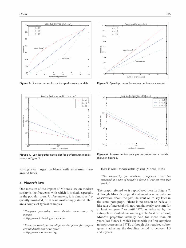
solving ever larger problems with increasing turn-around times.

4. Moore’s law

One measure of the impact of Moore’s law on modernsociety is the frequency with which it is cited, especiallyin the popular press. Unfortunately, it is almost as fre-quently misstated, or at least misleadingly stated. Hereare a couple of typical examples:

‘‘Computer processing power doubles about every 18

months.’’–http://www.technologyreview.com

‘‘Processor speeds, or overall processing power for comput-

ers will double every two years.’’–http://www.mooreslaw.org

Here is what Moore actually said (Moore, 1965):

‘‘The complexity for minimum component costs has

increased at a rate of roughly a factor of two per year (seegraph).’’

The graph referred to is reproduced here in Figure 7.Although Moore’s original statement was actually anobservation about the past, he went on to say later inthe same paragraph, ‘‘there is no reason to believe it[the rate of increase] will not remain nearly constant forat least ten years,’’ or until 1975, as indicated by theextrapolated dashed line on his graph. As it turned out,Moore’s projection actually held for more than 50years (see Figure 8, which begins with the first completemicroprocessors in 1971), although this required subse-quently adjusting the doubling period to between 1.5and 2 years.

Figure 4. Log–log performance plot for performance modelsshown in Figure 3.

Figure 6. Log–log performance plot for performance modelsshown in Figure 5.

Figure 3. Speedup curves for various performance models. Figure 5. Speedup curves for various performance models.

Heath 325

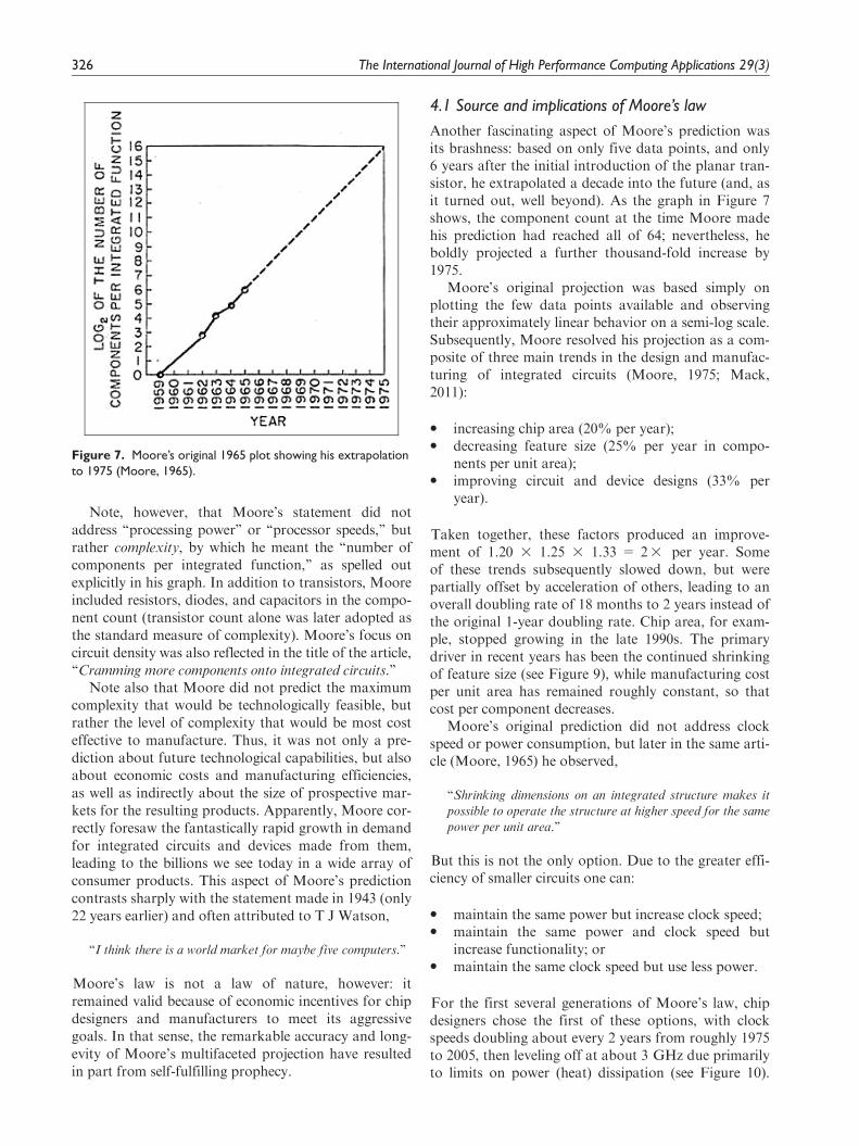
Note, however, that Moore’s statement did notaddress ‘‘processing power’’ or ‘‘processor speeds,’’ butrather complexity, by which he meant the ‘‘number ofcomponents per integrated function,’’ as spelled outexplicitly in his graph. In addition to transistors, Mooreincluded resistors, diodes, and capacitors in the compo-nent count (transistor count alone was later adopted asthe standard measure of complexity). Moore’s focus oncircuit density was also reflected in the title of the article,‘‘Cramming more components onto integrated circuits.’’

Note also that Moore did not predict the maximumcomplexity that would be technologically feasible, butrather the level of complexity that would be most costeffective to manufacture. Thus, it was not only a pre-diction about future technological capabilities, but alsoabout economic costs and manufacturing efficiencies,as well as indirectly about the size of prospective mar-kets for the resulting products. Apparently, Moore cor-rectly foresaw the fantastically rapid growth in demandfor integrated circuits and devices made from them,leading to the billions we see today in a wide array ofconsumer products. This aspect of Moore’s predictioncontrasts sharply with the statement made in 1943 (only22 years earlier) and often attributed to T J Watson,

‘‘I think there is a world market for maybe five computers.’’

Moore’s law is not a law of nature, however: itremained valid because of economic incentives for chipdesigners and manufacturers to meet its aggressivegoals. In that sense, the remarkable accuracy and long-evity of Moore’s multifaceted projection have resultedin part from self-fulfilling prophecy.

4.1 Source and implications of Moore’s law

Another fascinating aspect of Moore’s prediction wasits brashness: based on only five data points, and only6 years after the initial introduction of the planar tran-sistor, he extrapolated a decade into the future (and, asit turned out, well beyond). As the graph in Figure 7shows, the component count at the time Moore madehis prediction had reached all of 64; nevertheless, heboldly projected a further thousand-fold increase by1975.

Moore’s original projection was based simply onplotting the few data points available and observingtheir approximately linear behavior on a semi-log scale.Subsequently, Moore resolved his projection as a com-posite of three main trends in the design and manufac-turing of integrated circuits (Moore, 1975; Mack,2011):

� increasing chip area (20% per year);� decreasing feature size (25% per year in compo-

nents per unit area);� improving circuit and device designs (33% per

year).

Taken together, these factors produced an improve-ment of 1.20 3 1.25 3 1.33 = 23 per year. Someof these trends subsequently slowed down, but werepartially offset by acceleration of others, leading to anoverall doubling rate of 18 months to 2 years instead ofthe original 1-year doubling rate. Chip area, for exam-ple, stopped growing in the late 1990s. The primarydriver in recent years has been the continued shrinkingof feature size (see Figure 9), while manufacturing costper unit area has remained roughly constant, so thatcost per component decreases.

Moore’s original prediction did not address clockspeed or power consumption, but later in the same arti-cle (Moore, 1965) he observed,

‘‘Shrinking dimensions on an integrated structure makes it

possible to operate the structure at higher speed for the same

power per unit area.’’

But this is not the only option. Due to the greater effi-ciency of smaller circuits one can:

� maintain the same power but increase clock speed;� maintain the same power and clock speed but

increase functionality; or� maintain the same clock speed but use less power.

For the first several generations of Moore’s law, chipdesigners chose the first of these options, with clockspeeds doubling about every 2 years from roughly 1975to 2005, then leveling off at about 3 GHz due primarilyto limits on power (heat) dissipation (see Figure 10).

Figure 7. Moore’s original 1965 plot showing his extrapolationto 1975 (Moore, 1965).


Meanwhile, Moore’s original projection (concerningcomplexity, not speed) has continued to hold more orless to the present, although it too may be beginning towane. With clock speeds having leveled off, the secondoption has become the more recent trend, using thoseadditional transistors to increase functionality (e.g.multicore chips). With the advent of millions of mobiledevices, however, the third option (lower power) maybecome the dominant trend in order to prolong batterylife.

In 1974, near the end of the period of Moore’s origi-nal projection, these power issues were analyzed ingreater detail by Dennard et al. (1974), who observedthat both voltage and current scale proportionally withfeature size, so power scales proportionally with area,leading to a doubling of performance per watt approxi-mately every 2 years. Their analysis was specifically forMOSFETs (metal-oxide-semiconductor field-effecttransistors), but their conclusions were widely taken tobe generally applicable to integrated circuits morebroadly and were adopted by the semiconductor indus-try as a roadmap for future development. However, asfeature size continued to shrink in accordance withMoore’s law, this so-called Dennard scaling began tobreak down around 2005 due to increasing currentleakage and thermal noise, leading to the current stag-nation in clock speeds (Figure 10).

A more comprehensive study was undertaken byKoomey et al. (2010), who examined trends in powerconsumption since the beginning of electronic digitalcomputers with the ENIAC in 1946. Remarkably, thedata they collected for a wide variety of computers(mainframes, supercomputers, desktops, laptops, etc.)showed that energy efficiency, as measured by the num-ber of computations per unit of energy (kWh) dissi-pated, doubled every 1.57 years from 1946 to 2009 (seeFigure 11). Since a significant portion of their data wasfor computers that predated the advent of integrated

Figure 8. Plot of microprocessor transistor counts 1971–2011 showing continuation of Moore’s law (http://en.wikipedia.org/wiki/Moore’s_law).

Figure 9. Plot showing decreasing feature size of integratedcircuits in accordance with Moore’s law.

Heath 327

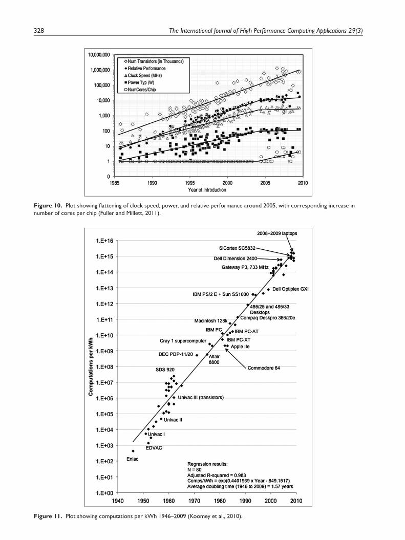
Figure 11. Plot showing computations per kWh 1946–2009 (Koomey et al., 2010).

Figure 10. Plot showing flattening of clock speed, power, and relative performance around 2005, with corresponding increase innumber of cores per chip (Fuller and Millett, 2011).


circuits, not all of the credit can be attributed toMoore’s law. Currently, GPUs (graphics processingunits) are continuing this doubling of performance perwatt with each new generation. And for mobile devicesthis means that for a fixed computing load the amountof battery required is approximately halved every yearand a half. Alas, this fortunate trend cannot continueindefinitely, as conventional computation cannot bemade arbitrarily energy efficient according to theLandauer limit (Landauer, 1961).

As we have seen, smaller transistors are better (cheaper,faster, lower power, more reliable), which enabled enor-mous gains in performance and cost effectiveness toaccompany the inexorable shrinking of feature size impliedby Moore’s law. Unfortunately, however, a threshold iseventually encountered below which smaller becomesworse rather than better, due to power dissipation, currentleakage, thermal noise, and ultimately quantum effects,thereby negating all of the advantages listed above exceptcheaper, and even that becomes questionable as more exo-tic materials and manufacturing processes are introducedin an attempt to prolong Moore’s law, which increasesmanufacturing costs in the bargain, exacerbating thealready exponential growth in the cost of fabrication facili-ties. Having now reached this threshold, the future fate ofMoore’s law has become less important, as the payofffrom further shrinking of feature size becomes increasinglymarginal instead of the pure win of the preceding era. Onecan debate whether or when Moore’s law has or will end,but in any case the 40-year free lunch appears to be over,regardless of whether another generation or two of shrink-age may prove to be possible at reasonable cost.

The relationships formulated by Moore and byDennard were destined to break down eventually, dueto both physical and economic constraints. When inter-est in large-scale parallel computing first arose in themid-1960s, reasons cited were often physical limits onsingle processor speeds, such as the speed-of-light limiton signal propagation, thereby forcing consideration ofparallel computing. Nevertheless, thanks to the trendsnoted by Moore and Dennard, single-processor speeds(and especially their cost effectiveness) continued toadvance exponentially for the next 40 years, confound-ing many early attempts at building commerciallyviable parallel computers. Ironically, when the day ofreckoning eventually came, it was barriers imposed by19th century physics (thermodynamics) rather than20th century physics (relativity and quantummechanics) that first proved insuperable.

The economic and societal impact of the 50-yearreign of Moore’s law is inestimable, with computersand other electronic devices now permeating everyaspect of daily life in a manner unimaginable 50 yearsago. To cite a familiar but telling example, the exponen-tial miniaturization, high performance, and low costthat followed from Moore’s law have made it possible

to buy for a few hundred dollars a cell phone that fits ina pocket and runs for days on battery power, yet has anorder of magnitude more processing power and mem-ory capacity than a US$10 million, 5.5 ton, 115 kWCray-1 supercomputer that was the world’s fastest from1976 until 1982. Whatever may lie ahead in the ‘‘post-Moore’’ era, we should be grateful that Moore’s lawpersisted long enough to provide the extreme degree ofinterconnectedness, information access, and productiv-ity enhancement that we now enjoy, not to mention theavailability of high-end computers for scientific com-puting at the petascale and beyond.

5. Epilogue

There has been an interesting interplay between Amdahl’slaw and Moore’s law throughout their mutual infancy,adolescence, and maturity. Consider the very first sentenceof Amdahl’s paper (Amdahl, 1967):

‘‘For over a decade prophets have voiced the contention that

the organization of a single computer has reached its limits

and that truly significant advances can be made only by

interconnection of a multiplicity of computers in such a man-

ner as to permit cooperative solution.’’

Amdahl’s deprecation of parallel processing was explicitlyintended to bolster the case for developing faster sequentialprocessing, as indicated by the title of his paper (‘‘Validityof the single processor approach .’’). Fortunately forAmdahl’s cause, Moore’s law would soon enable relentlessand relatively easy gains in single-processor performance,thereby forestalling successful commercial deployment ofparallel processing for decades.

Ironically, Amdahl’s first sentence eerily foresha-dowed the situation 40 years later when Dennard scalingground to a halt and parallel processing once againemerged as the answer to stagnating single-processor per-formance, but this time with much greater commercialsuccess, thanks to the additional processing cores thatMoore’s law could still deliver cheaply even if they couldnot run any faster. Amdahl may yet have the last laugh,however, as many of the impediments to effectivelyexploiting parallelism that he decried (irregular applica-tions, load imbalance, interprocessor coordination, slo-wed convergence rates, etc.) remain challenging today.

Acknowledgement

A preliminary version of this paper was presented as an invitedtalk at SC14 in New Orleans, Louisiana, 19 November 2014.

References

Amdahl GM (1967) Validity of the single processor approach

to achieving large scale computing capabilities. In: AFIPS

Spring joint computer conference, pp. 483–485.

Heath 329

Dennard RH, Gaensslen FH, Yu HN, Rideout VL, BassousE and LeBlanc AR (1974) Design of ion-implanted MOS-FET’s with very small physical dimensions. IEEE Journal

of Solid-State Circuits 9(5): 256–268.Fuller SH and Millett LI (eds.) (2011) The Future of Comput-

ing Performance: Game Over or Next Level? Washington,DC: National Academy of Sciences.

Grama A, Gupta A and Kumar V (1993) Isoefficiency: mea-suring the scalability of parallel algorithms and architec-tures. IEEE Parallel and Distributed Technology 1: 12–21.

Gustafson JL (1988) Reevaluating Amdahl’s law. Communi-

cations of the ACM 31: 532–533.Gustafson JL (1992) The consequences of fixed time perfor-

mance measurement. In: Proceedings of the twenty-fifth

Hawaii international conference on systems science

Hord RM (1982) The ILLIAC IV: The First Supercomputer.New York: Springer.

Karp AH and Flatt HP (1990) Measuring parallel processorperformance. Communications of the ACM 33: 539–543.

Koomey JG, Berard S, Sanchez M and Wong H (2010) Impli-cations of historical trends in the electrical efficiency ofcomputing. IEEE Annals of the History of Computing

33(3): 46–54.Landauer R (1961) Irreversibility and heat generation in the

computing process. IBM Journal of Research and Develop-

ment 5: 183–191.Mack CA (2011) Fifty years of Moore’s law. IEEE Transac-

tions on Semiconductor Manufacturing 24(2): 202–207.Moore GE (1965) Cramming more components onto inte-

grated circuits. Electronics 38(8): 114–117.

Moore GE (1975) Progress in digital integrated electronics.In: IEEE international electronic devices meeting, pp.11–13.

Singh JP, Hennessy JL and Gupta A (1993) Scaling parallelprograms for multiprocessors: methodology and examples.IEEE Computer 26(7): 42–50.

Van de Velde EF (1994) Concurrent Scientific Computing.New York: Springer.

Worley PH (1990) The effect of time constraints on scaledspeedup. SIAM Journal on Scientific and Statistical Com-puting 11: 838–858.

Author biography

Michael T Heath is Professor and Fulton WatsonCopp Chair Emeritus in the Department of ComputerScience at the University of Illinois at Urbana-Champaign. He received his Ph.D. in ComputerScience from Stanford University in 1978. His researchinterests are in scientific computing and parallel com-puting. He is an ACM Fellow, SIAM Fellow, AIAAAssociate Fellow, and a member of the EuropeanAcademy of Sciences. He received the Taylor L BoothEducation Award from the IEEE Computer Society in2009, and is author of the widely adopted textbookScientific Computing: An Introductory Survey, 2nd edi-tion, published by McGraw-Hill in 2002.


A tale of two laws -...

Documents

Transcript of A tale of two laws -...