A System Identi cation and Control Engineering … System Identi cation and Control Engineering...

A System Identification and Control Engineering Approach for Optimizing mHealth

Behavioral Interventions Based on Social Cognitive Theory

by

Cesar Antonio Martın Moreno

A Dissertation Presented in Partial Fulfillmentof the Requirements for the Degree

Doctor of Philosophy

Approved July 2016 by theGraduate Supervisory Committee:

Daniel E. Rivera, ChairEric B. Hekler

Matthew M. PeetKonstantinos S. Tsakalis

ARIZONA STATE UNIVERSITY

August 2016

ABSTRACT

Behavioral health problems such as physical inactivity are among the main causes

of mortality around the world. Mobile and wireless health (mHealth) interventions

offer the opportunity for applying control engineering concepts in behavioral change

settings. Social Cognitive Theory (SCT) is among the most influential theories of

health behavior and has been used as the conceptual basis of many behavioral inter-

ventions. This dissertation examines adaptive behavioral interventions for physical

inactivity problems based on SCT using system identification and control engineer-

ing principles. First, a dynamical model of SCT using fluid analogies is developed.

The model is used throughout the dissertation to evaluate system identification ap-

proaches and to develop control strategies based on Hybrid Model Predictive Control

(HMPC). An initial system identification informative experiment is designed to ob-

tain basic insights about the system. Based on the informative experimental results,

a second optimized experiment is developed as the solution of a formal constrained

optimization problem. The concept of Identification Test Monitoring (ITM) is devel-

oped for determining experimental duration and adjustments to the input signals in

real time. ITM relies on deterministic signals, such as multisines, and uncertainty re-

gions resulting from frequency domain transfer function estimation that is performed

during experimental execution. ITM is motivated by practical considerations in be-

havioral interventions; however, a generalized approach is presented for broad-based

multivariable application settings such as process control. Stopping criteria for the ex-

perimental test utilizing ITM are developed using both open-loop and robust control

considerations.

A closed-loop intensively adaptive intervention for physical activity is proposed re-

lying on a controller formulation based on HMPC. The discrete and logical features of

HMPC naturally address the categorical nature of the intervention components that

i

include behavioral goals and reward points. The intervention incorporates online

controller reconfiguration to manage the transition between the behavioral initiation

and maintenance training stages. Simulation results are presented to illustrate the

performance of the system using a model for a hypothetical participant under real-

istic conditions that include uncertainty. The contributions of this dissertation can

ultimately impact novel applications of cyberphysical system in medical applications.

ii

To my wife Rady and my daughters Isabella, Cristina and Bianca for all their love,

support and patience during our years in Tempe.

To my parents Ivonne and Cesar who have been my role-model for hard work,

persistence and dedication, and for transmitting me their visionary thoughts.

To my sisters Ivonne and Olguita for always being there with support and

motivation for all the family.

iii

ACKNOWLEDGMENTS

First and foremost, I would like to express my deepest gratitude to my advisor Dr.

Daniel E. Rivera for all his support, guidance, and understanding during these years.

His knowledge, dedication, patience, and approach to research have been fundamental

for the successful completion of this work. In particular I would like to thank him

for his dedication in reviewing my publications, and for teaching me how research

activities can be performed in effective and productive ways.

I would like to thank my committee members, Dr. Konstantinos Tsakalis, and

Dr. Matthew Peet for their support and comments on the content of this work,

which have been invaluable. My special thanks to Dr. Eric Hekler, who also serves

in my committee, for all his support, and for sharing with me his enthusiasm and

passion toward searching solutions for important behavioral health related problems.

Dr. Hekler proved to be a generous person, always willing to share his knowledge to

achieve greater scientific goals. I am also very grateful to Drs. William Riley, Matthew

Buman, and Marc Adams for sharing their knowledge, experience and views that were

fundamental for the construction of dynamical models that represent human behavior.

Additionally, I would like to extend my sincere gratitude to Drs. Konstantinos

Tsakalis, Hans Mittelmann, Daniel Rivera, Armando Rodriguez, Jennie Si, Walter

Higgins, and Ying-Cheng Lai for providing me with a solid foundation in the graduate

courses at ASU.

I wish to express gratitude to past and current members of the Control System

Engineering Lab (CSEL): Sunil Deshpande, Yuwen Dong, Kevin Timms, Penghong

Guo, Mohammad Freigoun, Gustavo Seixas, and Alicia Magann for all their support,

encouragement, and for the good times we had in the laboratory. It was important

to combine research activities with conversations about important things in life, and

occasional jovial moments.

iv

I am privileged for having such a wonderful and supportive family. My wife Rady,

and my daughters Isabella, Cristina and Bianca were responsible for make me feeling

always at home, regardless of the distance to our country. My parents Ivonne and

Cesar are my inspiration and motivation that made possible achieving this important

life goal. My sisters, parents in law, brother in law, and sisters in law have been very

supportive, always sending us good vibes that helped to obtain the strength to keep

going on with our plans.

This work would not have been possible without organizations which supported

my education, research, and development. My Ph.D. studies have been partially

supported by Escuela Superior Politecnica del Litoral (ESPOL) and Secretaria de

Educacion Superior, Ciencia, Tecnolgıa e Innovacion (SENESCYT) from Ecuador.

Support for this work has been provided by the National Science Foundation (NSF)

through grant IIS-1449751. Additional support has been received from the Piper

Health Solutions Consortium at Arizona State University. The opinions expressed in

this document are the author’s own and do not necessarily reflect the views of NSF

or the Virginia G. Piper Charitable Trust.

v

TABLE OF CONTENTS

Page

LIST OF TABLES . . . . . . . . . . . . . . . . . . . . . . . . . . . . . . . . . . . . . . . . . . . . . . . . . . . . . . . . . xi

LIST OF FIGURES . . . . . . . . . . . . . . . . . . . . . . . . . . . . . . . . . . . . . . . . . . . . . . . . . . . . . . . . xii

CHAPTER

1 INTRODUCTION . . . . . . . . . . . . . . . . . . . . . . . . . . . . . . . . . . . . . . . . . . . . . . . . . . . 1

1.1 Motivation . . . . . . . . . . . . . . . . . . . . . . . . . . . . . . . . . . . . . . . . . . . . . . . . . . . . . 1

1.2 Modeling Behavioral Theories . . . . . . . . . . . . . . . . . . . . . . . . . . . . . . . . . . . 3

1.3 Designing System Identification Experiments for Low Physical Ac-

tivity Behavioral Problems . . . . . . . . . . . . . . . . . . . . . . . . . . . . . . . . . . . . . . 7

1.4 Closed-loop Intensively Adaptive Intervention . . . . . . . . . . . . . . . . . . . . . 10

1.5 Research Goals . . . . . . . . . . . . . . . . . . . . . . . . . . . . . . . . . . . . . . . . . . . . . . . . . 12

1.5.1 Obtaining a Dynamical Model of SCT . . . . . . . . . . . . . . . . . . . . . 12

1.5.1.1 Basic SCT Model . . . . . . . . . . . . . . . . . . . . 12

1.5.1.2 Improvements to the SCT Model . . . . . . . . . . . 14

1.5.2 Designing System Identification Experiments . . . . . . . . . . . . . . . 16

1.5.2.1 Design of an Informative Experiment . . . . . . . . . 16

1.5.2.2 Design of an Optimized Experiment . . . . . . . . . 17

1.5.2.3 Redesign of the Informative Experiment Using an Iden-

tification Test Monitoring Approach . . . . . . . . . 20

1.5.3 Designing Closed-loop Interventions Relying on Hybrid Pre-

dictive Model Control Ideas . . . . . . . . . . . . . . . . . . . . . . . . . . . . . . . 25

1.6 Contributions of the Dissertation . . . . . . . . . . . . . . . . . . . . . . . . . . . . . . . . 28

1.7 Dissertation Outline . . . . . . . . . . . . . . . . . . . . . . . . . . . . . . . . . . . . . . . . . . . . 30

1.8 Publications . . . . . . . . . . . . . . . . . . . . . . . . . . . . . . . . . . . . . . . . . . . . . . . . . . . . 32

vi

CHAPTER Page

2 MODELING BEHAVIORAL INTERVENTIONS USING SOCIAL COG-

NITIVE THEORY. . . . . . . . . . . . . . . . . . . . . . . . . . . . . . . . . . . . . . . . . . . . . . . . . . . 36

2.1 Overview. . . . . . . . . . . . . . . . . . . . . . . . . . . . . . . . . . . . . . . . . . . . . . . . . . . . . . . 36

2.2 Social Cognitive Theory . . . . . . . . . . . . . . . . . . . . . . . . . . . . . . . . . . . . . . . . . 37

2.3 Developing a Fluid Analogy for SCT . . . . . . . . . . . . . . . . . . . . . . . . . . . . . 40

2.4 Dynamical Model Description . . . . . . . . . . . . . . . . . . . . . . . . . . . . . . . . . . . 44

2.4.1 Differential Equation Representation . . . . . . . . . . . . . . . . . . . . . . 45

2.4.2 Model Considerations . . . . . . . . . . . . . . . . . . . . . . . . . . . . . . . . . . . . 49

2.4.3 Stability Analysis . . . . . . . . . . . . . . . . . . . . . . . . . . . . . . . . . . . . . . . . 51

2.4.4 Nonlinear Dynamics of Habituation Within the SCT Model . 52

2.5 Illustrative Simulations . . . . . . . . . . . . . . . . . . . . . . . . . . . . . . . . . . . . . . . . . . 54

2.6 Semi-Physical Identification Using mHEALTH Intervention Data . . . 59

2.7 Model Improvements Based on a Physical Activity Behavioral In-

tervention . . . . . . . . . . . . . . . . . . . . . . . . . . . . . . . . . . . . . . . . . . . . . . . . . . . . . . 66

2.7.1 Description of the Intervention . . . . . . . . . . . . . . . . . . . . . . . . . . . . 67

2.7.2 Representing the Ideal Step-Goal Range Feature . . . . . . . . . . . 68

2.8 Chapter Summary . . . . . . . . . . . . . . . . . . . . . . . . . . . . . . . . . . . . . . . . . . . . . . 73

3 IDENTIFICATION TEST MONITORING PROCEDURE FOR MUL-

TIVARIABLE SYSTEMS . . . . . . . . . . . . . . . . . . . . . . . . . . . . . . . . . . . . . . . . . . . . 75

3.1 Overview. . . . . . . . . . . . . . . . . . . . . . . . . . . . . . . . . . . . . . . . . . . . . . . . . . . . . . . 75

3.2 Basic Identification Test Monitoring Procedure Based on Statistical

Uncertainty Estimates . . . . . . . . . . . . . . . . . . . . . . . . . . . . . . . . . . . . . . . . . . 78

3.2.1 Background and Input Signal Design . . . . . . . . . . . . . . . . . . . . . . 78

3.2.2 Uncertainty Description . . . . . . . . . . . . . . . . . . . . . . . . . . . . . . . . . . 84

vii

CHAPTER Page

3.2.2.1 Transfer Function Estimation . . . . . . . . . . . . . 84

3.2.2.2 Survey of Statistical Uncertainty Computation Methods 85

3.2.2.3 Additive Uncertainty Calculation . . . . . . . . . . . 87

3.2.2.4 Extension to a Parallel Connected System . . . . . . 89

3.2.2.5 Error-In-Variables Uncertainty Description . . . . . . 92

3.2.3 Derivation of a Monitoring Procedure . . . . . . . . . . . . . . . . . . . . . 94

3.3 Enhanced Identification Test Monitoring Procedure Relying on Un-

certainty Estimates . . . . . . . . . . . . . . . . . . . . . . . . . . . . . . . . . . . . . . . . . . . . . 96

3.3.1 Background . . . . . . . . . . . . . . . . . . . . . . . . . . . . . . . . . . . . . . . . . . . . . 96

3.3.1.1 The Local Polynomial Method . . . . . . . . . . . . 97

3.3.1.2 LPM for Arbitrary Excitations . . . . . . . . . . . . 99

3.3.1.3 LPM for Periodic Excitations . . . . . . . . . . . . . 101

3.3.2 Input Signal Design . . . . . . . . . . . . . . . . . . . . . . . . . . . . . . . . . . . . . . 106

3.3.2.1 Input Signals With “Zippered” Design . . . . . . . . 107

3.3.2.2 Input Signals With Full Design . . . . . . . . . . . . 110

3.3.3 Transfer Function and Uncertainty Computation . . . . . . . . . . . 112

3.3.4 Identification Test Monitoring Procedure . . . . . . . . . . . . . . . . . . 115

3.3.4.1 Aggregate Computation of Uncertainty . . . . . . . . 116

3.3.4.2 Stopping Criterion Based on Robustness Metrics . . 117

3.4 Simulation Study . . . . . . . . . . . . . . . . . . . . . . . . . . . . . . . . . . . . . . . . . . . . . . . 122

3.4.1 Basic Identification Test Monitoring Procedure . . . . . . . . . . . . . 123

3.4.2 Enhanced Identification Test Monitoring Procedure. . . . . . . . . 130

3.4.2.1 Simulation Results Using “Zippered” Signals . . . . . 132

3.4.2.2 Simulation Results Using Full Signals . . . . . . . . . 137

viii

CHAPTER Page

3.5 Chapter Summary . . . . . . . . . . . . . . . . . . . . . . . . . . . . . . . . . . . . . . . . . . . . . . 144

4 DESIGN OF OPEN-LOOP BEHAVIORAL INTERVENTIONS RELY-

ING ON SYSTEM IDENTIFICATION IDEAS . . . . . . . . . . . . . . . . . . . . . . . . 146

4.1 Overview. . . . . . . . . . . . . . . . . . . . . . . . . . . . . . . . . . . . . . . . . . . . . . . . . . . . . . . 146

4.2 Description of the Physical Activity Intervention and the System

Identification Problem . . . . . . . . . . . . . . . . . . . . . . . . . . . . . . . . . . . . . . . . . . 149

4.2.1 Simplified SCT Model . . . . . . . . . . . . . . . . . . . . . . . . . . . . . . . . . . . . 149

4.2.2 Intervention Components . . . . . . . . . . . . . . . . . . . . . . . . . . . . . . . . . 151

4.2.3 Grey-Box Parameter Estimation . . . . . . . . . . . . . . . . . . . . . . . . . . 155

4.2.4 General Design Constraints . . . . . . . . . . . . . . . . . . . . . . . . . . . . . . . 157

4.3 Informative Experimental Design . . . . . . . . . . . . . . . . . . . . . . . . . . . . . . . . 158

4.3.1 Randomized Signal Generation . . . . . . . . . . . . . . . . . . . . . . . . . . . . 158

4.3.2 Multisine Signal Generation . . . . . . . . . . . . . . . . . . . . . . . . . . . . . . 160

4.3.2.1 Basic Identification Test Monitoring Method . . . . . 160

4.3.2.2 Enhanced Identification Test Monitoring Method . . 168

4.4 Design of the Optimized Experiment . . . . . . . . . . . . . . . . . . . . . . . . . . . . . 181


4.5.1 Fixed Time Random Signal Experiments . . . . . . . . . . . . . . . . . . 186

4.5.2 Monitoring Process . . . . . . . . . . . . . . . . . . . . . . . . . . . . . . . . . . . . . . 193

4.5.2.1 Basic Identification Test Monitoring Procedure . . . 193

4.5.2.2 Enhanced Identification Test Monitoring Procedure . 201

4.6 Chapter Summary . . . . . . . . . . . . . . . . . . . . . . . . . . . . . . . . . . . . . . . . . . . . . . 209

5 DESIGN OF CLOSED-LOOP BEHAVIORAL INTERVENTIONS US-

ING HYBRID MODEL PREDICTIVE CONTROL . . . . . . . . . . . . . . . . . . . . 216

ix

CHAPTER Page

5.1 Overview. . . . . . . . . . . . . . . . . . . . . . . . . . . . . . . . . . . . . . . . . . . . . . . . . . . . . . . 216

5.2 Adaptive Closed-Loop Behavioral Intervention Based on SCT . . . . . . 218

5.3 Formulation of the HMPC-Based Adaptive Intervention . . . . . . . . . . . 220

5.3.1 Use of the HMPC framework . . . . . . . . . . . . . . . . . . . . . . . . . . . . . 221

5.3.2 Discrete and Logical Constraints . . . . . . . . . . . . . . . . . . . . . . . . . . 229

5.3.3 Maintenance Training Stage . . . . . . . . . . . . . . . . . . . . . . . . . . . . . . 231


5.5 Chapter summary . . . . . . . . . . . . . . . . . . . . . . . . . . . . . . . . . . . . . . . . . . . . . . 246

6 SUMMARY AND FUTURE WORK . . . . . . . . . . . . . . . . . . . . . . . . . . . . . . . . . . 247

6.1 Summary of the Dissertation . . . . . . . . . . . . . . . . . . . . . . . . . . . . . . . . . . . . 247

6.2 Directions for Future Work . . . . . . . . . . . . . . . . . . . . . . . . . . . . . . . . . . . . . . 253

6.2.1 “Just in Time” Adaptive Interventions . . . . . . . . . . . . . . . . . . . . 253

6.2.2 Enhancements to System Identification Experiments . . . . . . . . 254

6.2.3 Improvements to the Identification Test Monitoring Procedure257

6.2.4 Reconfiguration of the Semiphysical Identification Procedure 258

6.2.5 General Ideas . . . . . . . . . . . . . . . . . . . . . . . . . . . . . . . . . . . . . . . . . . . . 259

REFERENCES . . . . . . . . . . . . . . . . . . . . . . . . . . . . . . . . . . . . . . . . . . . . . . . . . . . . . . . . . . . . 260

x

LIST OF TABLES

Table Page

2.1 Lookup Table for β46 . . . . . . . . . . . . . . . . . . . . . . . . . . . . . . . . . . . . . . . . . . . . . . . 54

4.1 Constant Values of Design Constraints for Informative and Optimized

Experiments. . . . . . . . . . . . . . . . . . . . . . . . . . . . . . . . . . . . . . . . . . . . . . . . . . . . . . . 187

4.2 Performance Metrics Comparison of Input/output Signals From Infor-

mative and Optimized Experiments. . . . . . . . . . . . . . . . . . . . . . . . . . . . . . . . . 193

4.3 Monitoring Indexes of the Informative Experiment for the Input/output

Direction of Interest [4, 8]. . . . . . . . . . . . . . . . . . . . . . . . . . . . . . . . . . . . . . . . . . 197

4.4 Performance Metrics Comparison of Input/output Signals From Infor-

mative and Optimized Experiments Resulting From the Basic Moni-

toring Process. . . . . . . . . . . . . . . . . . . . . . . . . . . . . . . . . . . . . . . . . . . . . . . . . . . . . 200

4.5 Percentages of Uncertainty Reduction According to (4.105) – (4.106)

for Increments on the Amplitude of the Input Signals. . . . . . . . . . . . . . . . 208

4.6 Percentages of Uncertainty Reduction According to (4.105) – (4.106)

for Changes on the Frequency Content of the Input Signals. . . . . . . . . . . 208

4.7 Performance Metrics Comparison of Input/output Signals From In-

formative and Optimized Experiments Resulting From the Enhanced

Monitoring Process. . . . . . . . . . . . . . . . . . . . . . . . . . . . . . . . . . . . . . . . . . . . . . . . 211

xi

LIST OF FIGURES

Figure Page

1.1 Conceptual Schematic of the Social Cognitive Theory (SCT), as Pre-

sented in Bandura (2004). . . . . . . . . . . . . . . . . . . . . . . . . . . . . . . . . . . . . . . . . . . 5

1.2 Fluid Analogy for the Theory of Planned Behavior (TPB) Presented by

Navarro-Barrientos et al. (2011). PBC Stands for Perceived Behavioral

Control. . . . . . . . . . . . . . . . . . . . . . . . . . . . . . . . . . . . . . . . . . . . . . . . . . . . . . . . . . . 6

1.3 Three Legged Stool Analogy for Intensively Adaptive Interventions

(IAI; Riley et al. (2015b)). . . . . . . . . . . . . . . . . . . . . . . . . . . . . . . . . . . . . . . . . . . 8

1.4 Conceptual Representation of the Open-Loop IAI Components Acting

on the SCT Model. . . . . . . . . . . . . . . . . . . . . . . . . . . . . . . . . . . . . . . . . . . . . . . . . 9

1.5 Conceptual Diagram of the Closed-Loop IAI Over the SCT Model. . . . 11

1.6 Proposed Fluid Analogy for Social Cognitive Theory. . . . . . . . . . . . . . . . . . 13

1.7 Hypothetical Representation of the Inverted U for a Physical Activity

Behavioral Problem Showing Step-Goals and Actual Steps. . . . . . . . . . . . 14

1.8 Proposed Improvement to the SCT Model to Incorporate the Ideal

Step-Goal Range Feature Over the Intensively Adaptive Intervention

(IAI). . . . . . . . . . . . . . . . . . . . . . . . . . . . . . . . . . . . . . . . . . . . . . . . . . . . . . . . . . . . . . 15

1.9 Conceptual Representation of the “If/Then” Block That Defines the

Deliverance of Reward Points in Dependence of the Goal Attainment. . 19

1.10 Representation of Statistical Confidence Regions for a Given Proba-

bility at Each Frequency Point, Based on Additive Uncertainties for

Transfer Function Estimates G and Presented Over a Nyquist Plot. . . . 21

1.11 Block Diagram of a Closed-Loop System Subject to Additive Uncer-

tainty LA = ¯a ·∆a. . . . . . . . . . . . . . . . . . . . . . . . . . . . . . . . . . . . . . . . . . . . . . . . . 24

xii

Figure Page

1.12 Conceptual Representation of the Receding Horizon Control Strategy

to the Physical Activity Behavioral Problem With Control Moves Com-

puted Only for Step Goals (u8), and Considering Steps (y4) as the Out-

put and Environmental Context (d7 = ξ7) as a Measured Disturbance. . 26

2.1 Triadic Reciprocal Determinism of Social Cognitive Theory. . . . . . . . . . . . 38

2.2 Fluid Analogy for Social Cognitive Theory, Augmented With Habitu-

ation. . . . . . . . . . . . . . . . . . . . . . . . . . . . . . . . . . . . . . . . . . . . . . . . . . . . . . . . . . . . . . 41

2.3 Path Diagram for Social Cognitive Theory Derived From the Fluid

Analogy. . . . . . . . . . . . . . . . . . . . . . . . . . . . . . . . . . . . . . . . . . . . . . . . . . . . . . . . . . . 44

2.4 Self-Management Skills Inventory (η1) Showing All its Inflows and Out-

flows . . . . . . . . . . . . . . . . . . . . . . . . . . . . . . . . . . . . . . . . . . . . . . . . . . . . . . . . . . . . . . 46

2.5 Inventory Cue to Action (η6) With the Addition of a Feedback Con-

troller to Represent a Second Order System. . . . . . . . . . . . . . . . . . . . . . . . . . 47

2.6 Block Diagram for a Second Order Inventory System. . . . . . . . . . . . . . . . . . 48

2.7 Gain Schedule Illustration for β46 . . . . . . . . . . . . . . . . . . . . . . . . . . . . . . . . . . . 55

2.8 Scenario 1: Failure on the Initiation of Physical Activity Behavior

Under Low Self-Efficacy and in the Presence of External Cues. . . . . . . . 56

2.9 Scenario 2: Success of Initiation and Maintenance of Physical Activity

Behavior Under High Self-Efficacy and in the Presence of External

Cues and Additional Internal Cues. . . . . . . . . . . . . . . . . . . . . . . . . . . . . . . . . 57

2.10 Scenario 3: Maintenance of Physical Activity Behavior Under High

Self-Efficacy and a Model Depicting a Higher Degree of Integration. . . 58

xiii

Figure Page

2.11 Scenario 4: Behavior Under a Persistent External Cue That Causes

Habituation and Later Recovery After the Stimulus is Removed. High

Self-Efficacy Conditions are Considered. Two Plots for Behavior are

Shown: One Following a Linear Response (With no Habituation Con-

sidered), the Other Using the Proposed Model With a Nonlinear Block. 59

2.12 Scenario 5: Behavior Under a Higher External Cue (More Frequent

Stimulus) That Causes Habituation and a Later Recovery Once the

Stimulus Is Removed. Conditions of High Self-Efficacy are Considered. 60

2.13 MILES Data Averaged for a Subset of Six Participants With the Re-

quired Signals for Raw Daily Sampling and Weekly Average Including

95 % Confidence Intervals. . . . . . . . . . . . . . . . . . . . . . . . . . . . . . . . . . . . . . . . . . . 62

2.14 SCT Model Subsystem Used for Semiphysical Identification With the

MILES Data. . . . . . . . . . . . . . . . . . . . . . . . . . . . . . . . . . . . . . . . . . . . . . . . . . . . . . 63

2.15 Data From MILES Study (Solid Line) Contrasted Against Simulation

Results From the Model (Dotted Line) Considering the Same Input

Values for Both Scenarios. . . . . . . . . . . . . . . . . . . . . . . . . . . . . . . . . . . . . . . . . . 65

2.16 Conceptual Representation of the Physical Activity Intervention, Based

on a Simplified Version of the SCT Model. . . . . . . . . . . . . . . . . . . . . . . . . . . 68

2.17 Hypothetical Steady State Equilibrium Curve Where the X-Axis Cor-

responds to the Recommended Goals (ξ8), and the Y-Axis Gives the

Actual Performed Steps (η4) and Self-efficacy (η3). . . . . . . . . . . . . . . . . . . 69

2.18 Low Physical Activity Intervention Based on the Simplified SCT Model

With Reincorporation of the Self-Efficacy Inventory η3 to Implement

the Ideal Range Goal-Setting Feature. . . . . . . . . . . . . . . . . . . . . . . . . . . . . . . . 70

xiv

Figure Page

2.19 Simulation Results for a Physical Activity Behavioral Intervention,

Representing the Ideal Range of Step-Goals Feature by Influencing

Self-Efficacy (η3) Through the Goal Attainment (u11) Signal. . . . . . . . . . 72

3.1 Block Diagram for the MIMO System Describing the Effect of an In-

dividual SISO Transfer Function G[m,n] Over the Outputs. . . . . . . . . . . . 79

3.2 Conceptual Representation for a nu = 2 Channel “Zippered” Spectra

Design With ns = 6 Independently Excited Sinusoids, Giving nh = 6

Harmonics and Selecting Ns = 18. . . . . . . . . . . . . . . . . . . . . . . . . . . . . . . . . . . 81

3.3 Conceptual Representation of the 100 × (1 − ρ)% Confidence Region

for G[m,n](ωni ) Over a Nyquist Frequency Response Plot for a Specific

Frequency ωni ∈W n. . . . . . . . . . . . . . . . . . . . . . . . . . . . . . . . . . . . . . . . . . . . . . . 86

3.4 Block Diagram of a Modified System Including the Effect of a Transfer

Function S[m,n](q) Connected in Parallel With G[m,n](q). . . . . . . . . . . . . . . 90

3.5 Block Diagram Showing the Error-In-Variable Setting for Input n and

Output m of a MIMO System. . . . . . . . . . . . . . . . . . . . . . . . . . . . . . . . . . . . . . . 93

3.6 Excited and Non-Excited Frequency Components According to the Pe-

riodic LPM, Where Solid Lines Correspond to the System Response

and Dashed Lines are the Transient and Noise Contributions. . . . . . . . . . 101

3.7 Conceptual Representation of the Desired “Zippered” and Harmonic

Related Spectra for nu = 2 Input Signals. The X-Axis Represents

the Harmonic Frequencies ωj While the Y-axis Represents the Fourier

Coefficients αn,l,j. . . . . . . . . . . . . . . . . . . . . . . . . . . . . . . . . . . . . . . . . . . . . . . . . . 109

xv

Figure Page

3.8 Conceptual Representation of the Desired Harmonic Related Spectra

for nu = 2 Input Signals With the Full Design. The X-Axis Represents

the Harmonic Frequencies ωj While the Y-Axis Represents the Fourier

Coefficients αn,l,j. . . . . . . . . . . . . . . . . . . . . . . . . . . . . . . . . . . . . . . . . . . . . . . . . . 112

3.9 Closed-Loop Representation of the System Describing a Single Un-

structured Additive Uncertainty. . . . . . . . . . . . . . . . . . . . . . . . . . . . . . . . . . . . 118

3.10 Inverse Performance Weight 1/|wP | Used for Robust Performance Test

According to (3.178). . . . . . . . . . . . . . . . . . . . . . . . . . . . . . . . . . . . . . . . . . . . . . . 120

3.11 Simulation Results for the Model Defined in (3.188) With M = 2 Peri-

ods of Input Signals and Considering v1 ∼ N (0, 1) and v2 ∼ N (0, .3).

. . . . . . . . . . . . . . . . . . . . . . . . . . . . . . . . . . . . . . . . . . . . . . . . . . . . . . . . . . . . . . . . . . 124

3.12 Additive Uncertainties `1−ρa[1,2](ω

ni ,M) Drawn as Circles Around the ET-

FEs for G[1,2], with ρ = 0.5, σ21 = 1, σ2

2 = 0.3, M = 15 Periods and

Showing 100 Replications With Different Noise Realizations. . . . . . . . . . . 125

3.13 Illustration of the Monitoring Procedure With Estimates Made for

M = 1, . . . 11, m = 1, 2 and n = 1, 2 and Showing Values of ˜a[m,n](M),

AV[m,n](M), RV[m,n](M), and %e[m,n](M). . . . . . . . . . . . . . . . . . . . . . . . . . . . . 126

3.14 Nyquist Plots of ETFEs G[m,n](ωni ,M) for all the Input Output El-

ements Compared to the Simulation Plant G[m,n](ωni ), Including the

Percentage Mean Error %e[m,n](M) After Stopping the Experiment at

M = 10 Periods. . . . . . . . . . . . . . . . . . . . . . . . . . . . . . . . . . . . . . . . . . . . . . . . . . . . 127

3.15 Estimated Additive Uncertainties for 10 Replications of Gaussian Out-

put Noise With σ21 = 1 and σ2

2 = 0.3 for M = 2, . . . , 14. Percentage

Mean Errors for Each Case are Also Shown. . . . . . . . . . . . . . . . . . . . . . . . . . 128

xvi

Figure Page

3.16 Monitoring Procedure Assuming an Autoregressive Output Noise With

σ21 = 0.2, σ2

2 = 0.1 and φ = 0.6, Including Uncertainty Estimates and

Percentage Mean Error Computations. . . . . . . . . . . . . . . . . . . . . . . . . . . . . . . 128

3.17 Monitoring Procedure Assuming an Integral Output Noise With σ21 =

0.2, σ22 = 0.1, and φ = 0.9 Including Uncertainty Estimations and

Percentage Mean Error Computations. . . . . . . . . . . . . . . . . . . . . . . . . . . . . . . 129

3.18 Estimated Additive Uncertainties for 10 Replications of Autoregressive

and Integral Noise for M = 2, . . . , 62. Percentage Mean Errors for Each

Case are Also Shown. . . . . . . . . . . . . . . . . . . . . . . . . . . . . . . . . . . . . . . . . . . . . . 130

3.19 Illustration of the Proposed Simple Search Procedure for the Values λ∗1

and λ∗2 That Minimizes RPiMax. . . . . . . . . . . . . . . . . . . . . . . . . . . . . . . . . . . . 132

3.20 Simulation of Input Signals Designed With the “Zippered” Method

and the Resulting Output Signals for M = 2 Cycles With σ21 = 1 and

σ22 = 0.3. . . . . . . . . . . . . . . . . . . . . . . . . . . . . . . . . . . . . . . . . . . . . . . . . . . . . . . . . . . 133

3.21 Additive Uncertainties for the “Zippered” Design Drawn as Circular

Regions Around Each Real Transfer Function Response, Showing Dif-

ferent Transfer Function Estimates for 100 Realizations of the Same

Gaussian Noise. . . . . . . . . . . . . . . . . . . . . . . . . . . . . . . . . . . . . . . . . . . . . . . . . . . . 133

3.22 Illustration of the Monitoring Process for M = 1, · · · , 16 Cycles of the

Same Input Signals With no Modifications. Uncertainties and Robust

Performance Indexes Are Computed for ρ = 0.05 . . . . . . . . . . . . . . . . . . . . . 135

3.23 Simulation of the “Zippered” Experiment Considering a Total ofM = 3

Cycles, and Including a Change on the Input Amplitude After M = 2

Cycles. . . . . . . . . . . . . . . . . . . . . . . . . . . . . . . . . . . . . . . . . . . . . . . . . . . . . . . . . . . . 135

xvii

Figure Page

3.24 Simulation of the “Zippered” Experiment Considering a Total ofM = 3

Cycles, and Including a Change on the Fundamental Frequency of the

Inputs After M = 2 Cycles. . . . . . . . . . . . . . . . . . . . . . . . . . . . . . . . . . . . . . . . . . 136

3.25 Illustration of the Monitoring Process for M = 1, · · · , 16 Cycles Con-

sidering Changes in the Amplitude and the Frequency Content of the

Input Signals After M = 6 Cycles. . . . . . . . . . . . . . . . . . . . . . . . . . . . . . . . . . 137

3.26 Ten Computations of the Robust Performance Index and the Abso-

lute Mean Error Relying on the “Zippered” Design Generated From

Different Realizations of Gaussian Noise With σ21 = 1, and σ2

2 = 0.3. . . 138

3.27 Illustration of 10 Independent Computations of RPiMax and e Using

Different Noise Structures for the “Zippered” Design: 1) Autoregres-

sive With φ = 0.6, σ21 = 0.2, and σ2

2 = 0.1. 2) Integral With φ = 0.9,

σ21 = 0.2, and σ2

2 = 0.1. . . . . . . . . . . . . . . . . . . . . . . . . . . . . . . . . . . . . . . . . . . . . 139

3.28 Simulation of Input Signals Designed With the Full Method and the

Resulting Output Signals for M = 2 Cycles With σ21 = 1 and σ2

2 = 0.3. 139

3.29 Additive Uncertainties for the Full Design Drawn As Circular Re-

gions Around Each Real Transfer Function Response, Showing Dif-

ferent Transfer Function Estimates for 100 Realizations of the Same

Gaussian Noise. . . . . . . . . . . . . . . . . . . . . . . . . . . . . . . . . . . . . . . . . . . . . . . . . . . . 140

3.30 Original Additive Uncertainties ε1−κ(ωn,M) Computed Using the Full

Design for M = 3 Cycles, With Corresponding Reduction to Neglect

the Border Effect. . . . . . . . . . . . . . . . . . . . . . . . . . . . . . . . . . . . . . . . . . . . . . . . . . 141

xviii

Figure Page

3.31 Illustration of the Monitoring Process for M = 1, · · · , 16 Cycles of the

Same Input Signals With No Modifications. Uncertainties and Robust

Performance Indexes Are Computed for ρ = 0.05. . . . . . . . . . . . . . . . . . . . . 142

3.32 Ten Computations of the Robust Performance Index and the Abso-

lute Mean Error Relying on the Full Design Generated From Different

Realizations of Gaussian Noise With σ21 = 1, and σ2

2 = 0.3. . . . . . . . . . . . 142

3.33 Illustration of the Monitoring Process for M = 1, · · · , 16 Cycles Con-

sidering Changes in the Amplitude and the Frequency Content of the

Input Signals After M = 6 Cycles. . . . . . . . . . . . . . . . . . . . . . . . . . . . . . . . . . 143

3.34 Illustration of 10 Independent Computations of RPiMax and e Using

Different Noise Structures for the Full Design: 1) Autoregressive With

φ = 0.6, σ21 = 0.2, and σ2

2 = 0.1. 2) Integral With φ = 0.9, σ21 = 0.2,

and σ22 = 0.1. . . . . . . . . . . . . . . . . . . . . . . . . . . . . . . . . . . . . . . . . . . . . . . . . . . . . . . 143

4.1 Fluid Analogy for a Simplified Version of the SCT Model Developed

in Chapter 2. . . . . . . . . . . . . . . . . . . . . . . . . . . . . . . . . . . . . . . . . . . . . . . . . . . . . . . 150

4.2 Conceptual Diagram for the Proposed Intervention to Influence Behav-

ior and Other Constructs Represented by the Simplified SCT Model.

Input/output Symbols ξi and ηi are Used for Modeling and Simula-

tion, While ui and yi are Used for Formulations of the Informative and

Optimized Experiments. . . . . . . . . . . . . . . . . . . . . . . . . . . . . . . . . . . . . . . . . . . . 152

4.3 Block Diagram Representing the IMC Design Structure for the Self-

Regulator Via Internalized Cues. . . . . . . . . . . . . . . . . . . . . . . . . . . . . . . . . . . . 153

xix

Figure Page

4.4 Block Diagram for the Physical Activity Behavioral Intervention Based

on the Simplified SCT Model, Using Independent Transfer Functions

for Each Input/output Element. . . . . . . . . . . . . . . . . . . . . . . . . . . . . . . . . . . . . 163

4.5 Representation of the “If/Then” Block, Using Relay-Type and Dead-

Zone Nonlinearities. . . . . . . . . . . . . . . . . . . . . . . . . . . . . . . . . . . . . . . . . . . . . . . . . 164

4.6 Block Diagram for the Transfer Function G[4,8](q) From u8 to y4 Ne-

glecting the Effect of u9. . . . . . . . . . . . . . . . . . . . . . . . . . . . . . . . . . . . . . . . . . . . . 165

4.7 Realization of the Desired Behavior (ydes) to be Used in the Formula-

tion of the Optimized Experiment, With a Starting Baseline of 5, 000

Steps, and a Duration of 273 Days. . . . . . . . . . . . . . . . . . . . . . . . . . . . . . . . . . 183

4.8 Input/output Data for the Fixed Time Informative Experiment Using

Random Inputs Within Clinical Constraints. . . . . . . . . . . . . . . . . . . . . . . . . 188

4.9 Cross-Validation Results Comparing the Simulation Plant With the

Identified Model From the Informative Experiment. . . . . . . . . . . . . . . . . . 190

4.10 Input/output Data for the Fixed Time Optimized Experiment. . . . . . . . 191


Identified Model From the Informative and Optimized Experiments. . . 192

4.12 Simulation Results Using the “Simulation Plant” and the Designed

Multisine With “Zippered” Spectra Signals for M=5 Periods. . . . . . . . . 194

4.13 Nyquist Plot of G[m,n](ω) (n = 8, 9 and m = 4, 5) for Ns = 18, ns = 8

and M = 50 Periods, With 95% Additive Uncertainty Bounds Drawn

as Circumferences Over Each Frequency Estimate and Showing 100

Replications. . . . . . . . . . . . . . . . . . . . . . . . . . . . . . . . . . . . . . . . . . . . . . . . . . . . . . . 195

xx

Figure Page

4.14 Additive Uncertainty Bound Estimates ã[m,n](M) With Percentages of

Variation for M = 3, . . . , 16. Percentages of fit to a Cross-Validation

Data set for y4 and y5 are Also Plotted. Results are Computed Only

for the Input/output Direction of Interest [4, 8]. . . . . . . . . . . . . . . . . . . . . . 196

4.15 Estimates of ã[4,8](M) and %fit4 for a set of 10 Different Realizations

of Output Gaussian Noise v4(k) and v5(k) With σ24 = 300000, σ2

5 = 500. 198

4.16 Estimates of ã[4,8](M) and %fit4 for a set of 10 Different Realizations

of two Types of Noise for v4(k): Autoregressive With σ24 = 300000,

φ = 0.7, and Integral With σ24 = 300000, and φ = 0.9. . . . . . . . . . . . . . . . . . 199

4.17 Input/output Data for the Optimized Experiment Derived From the

Basic Monitoring Procedure. . . . . . . . . . . . . . . . . . . . . . . . . . . . . . . . . . . . . . . . 200


Identified Model From the Informative and Optimized Experiments

Resulting From the Basic Monitoring Process. . . . . . . . . . . . . . . . . . . . . . . . 201

4.19 Simulation Results Using the “Simulation Plant” and the Designed

Multisine With “Zippered” Spectra Signals for M=5 Periods to be

Used in the Enhanced Monitoring Process. . . . . . . . . . . . . . . . . . . . . . . . . . . 202

4.20 Additive Uncertainties à[m,n](ωn,l,i) Correspondent to Each Frequency

Transfer Function Estimate, Drawn as Circular Regions Around Each

Noiseless Estimate, With 100 Replications of the Same Gaussian Noise

(σ24 = 300000 and σ2

5 = 500) for the Enhanced Monitoring Process. . . . 203

4.21 Evaluation of the Enhanced Identification Test Monitoring Process for

a Simulation Plant With no Changes in the Amplitude and/or Fre-

quency Content of the Input Signals, at Each Cycle M = 1, · · · , 16. . . . . 204

xxi

Figure Page

4.22 Illustration of the Different Types of Changes in the Inputs Signal

Content for the Enhanced Monitoring Method After M = 5 Cycles

With a Total of M = 8 Cycles. . . . . . . . . . . . . . . . . . . . . . . . . . . . . . . . . . . . . . 205

4.23 Illustration of the Enhanced Identification Test Monitoring Method,

Testing all the Possible Actions Over the Input Signals After M = 5

Cycles: no Changes, Increments on the Amplitude, and Changes on

the Harmonic Related Frequencies for M = 1, · · · , 16. . . . . . . . . . . . . . . . . 207

4.24 Ten Replications of the Enhanced Monitoring Process for Different

Noise Structures, Including Gaussian With σ24 = 300000, σ2

5 = 500,

Autoregressive With σ24 = 300000 and φ = 0.7, and Integral With

σ24 = 300000, and φ = 0.9. . . . . . . . . . . . . . . . . . . . . . . . . . . . . . . . . . . . . . . . . . 210

4.25 Input/output Data for the Optimized Experiment Derived From the

Enhanced Monitoring Process. . . . . . . . . . . . . . . . . . . . . . . . . . . . . . . . . . . . . . . 211


Identified Model From the Informative and Optimized Experiments

Resulting From the Enhanced Monitoring Process. . . . . . . . . . . . . . . . . . . 212

4.27 Comparison Between the Computed MIMO Additive Uncertainties

ε(M) for the Basic and Enhanced Monitoring Procedures Applied Over

the Same Input Signals. . . . . . . . . . . . . . . . . . . . . . . . . . . . . . . . . . . . . . . . . . . . 215

5.1 Conceptual Representation of the Closed-Loop Behavioral Adaptive

Intervention, Based on the Simplified Version of the SCT Model in

Fig. 4.1 . . . . . . . . . . . . . . . . . . . . . . . . . . . . . . . . . . . . . . . . . . . . . . . . . . . . . . . . . . . 219

xxii

Figure Page

5.2 Conceptual Application of the Receding Horizon Control Strategy to

the Physical Activity Behavioral Problem Considering Step Goals (u8)

as the Input, Actual Steps (y4) as the Output, and Environmental

Context (d7) as Measured Disturbance. . . . . . . . . . . . . . . . . . . . . . . . . . . . . . . 223

5.3 Block Diagram Depicting the Three Degree-of-Freedom Tuning Within

the HMPC Formulation. P and Pd Are the System Plant Models,

X(k/k), Kf is the Observer Block, Y(k + 1) is the Predictor Block,

F (q, αx), x = r, d are the Filters for Reference and Measured Distur-

bance Signals, and the Block Referred as “min J” is the Optimizer

Where ρ is the Vector of Decision Variables. . . . . . . . . . . . . . . . . . . . . . . . . 227

5.4 Simulation Results for the HMPC Based Adaptive Intervention for a

Participant With low Physical Activity, Considering d′(K) ∼ N (0, 40000),

wu9 = 0.005, αr = [0 0 .96 0]T , αd = 0.1, and fa = [0 0 0.3 0]T . 235

5.5 Performance of the HMPC Physical Activity Intervention Versus a

Self-Regulation via Internalized Cues Case With a Pre-Defined Set of

Incremental Step Goals. . . . . . . . . . . . . . . . . . . . . . . . . . . . . . . . . . . . . . . . . . . . . 236



wu9 = 0.005, αr = [0 0 .96 0]t, αd = 0.1, and fa = [0 0 0.3 0]T . 237



αr = [0 0 .96 0]T , αd = 0.1, fa = [0 0 .3 0]t, and two Different

Cases for wu9 : wu9 = 0.05, and wu9 = 0.0005. . . . . . . . . . . . . . . . . . . . . . . . . . 238

xxiii

Figure Page

5.8 More detailed comparison of results from Fig. 5.7 considering only the

time interval where the first maintenance phase occurs, and including

the computation of 2-norms (‖un‖2) for the manipulated inputs and

the output behavior (u8, u9, u10, and y4) for each value of wu9 . . . . . . . . . 239

5.9 Evaluation of the Three Degree-of-Freedom Tuning Procedure Over

the Output y4, Considering Three Different Scenarios. . . . . . . . . . . . . . . . 240

5.10 Evaluation of the Three Degree-of-Freedom Tuning Procedure Over

the Inputs u8 and u9, Considering Three Different Scenarios. . . . . . . . . . 241

5.11 Performance of the HMPC Based Intervention for Different Scenarios

of Positive Plant-Model Mismatch, With no Unmeasured Disturbance

Considered. . . . . . . . . . . . . . . . . . . . . . . . . . . . . . . . . . . . . . . . . . . . . . . . . . . . . . . . 242

5.12 Performance of the HMPC Based Intervention for Different Scenarios

of Negative Plant-Model Mismatch, With no Unmeasured Disturbance

Considered. . . . . . . . . . . . . . . . . . . . . . . . . . . . . . . . . . . . . . . . . . . . . . . . . . . . . . . . 243

5.13 Performance of the HMPC Based Intervention for Different Scenar-

ios of Positive/negative Plant-Model Mismatch, With no Unmeasured

Disturbance Considered. . . . . . . . . . . . . . . . . . . . . . . . . . . . . . . . . . . . . . . . . . . . 244

5.14 Performance of the HMPC Based Intervention for Different Scenarios of

Positive/negative Plant-Model Mismatch, With αd = 0.9 and f 3a = 0.01.245

6.1 Comprehensive Illustration of a Representative Time Series Resulting

From the “Just Walk” Intervention That Features Three Phases: Iden-

tification Testing, Initiation and Maintenance. . . . . . . . . . . . . . . . . . . . . . . . 252

6.2 Conceptual Block Diagram Representation of a Multi-Timescales JIT

Adaptive Intervention. . . . . . . . . . . . . . . . . . . . . . . . . . . . . . . . . . . . . . . . . . . . . 255

xxiv

Figure Page

6.3 Block Diagram for the Physical Activity Behavioral Considering Inde-

pendent Transfer Functions for Each Input/output Element. . . . . . . . . . 257

xxv

Chapter 1

INTRODUCTION

1.1 Motivation

Control system engineering principles have been applied in a diverse series of

fields. These go beyond mechanical, chemical, civil and electrical engineering, to

include the social and natural sciences in important problems involving economic,

environmental and biological systems, among others. One key advantage of a control

system representation of systems is its ability to support the design of a model-based

controller that can manipulate the system response to accomplish a desired goal.

Health is a major concern in society; therefore significant research efforts have

focused on this problem. Many infectious diseases are under control in developed

countries, creating the need to address behavioral health problems. For example,

three behavioral risk factors - tobacco use, poor diet, and inactivity - contribute

to four major chronic diseases: heart disease, type 2 diabetes, lung disease, and

cancer. Together, these behaviors account for more than 50% of preventable deaths

(Hekler et al., 2013b). Given these facts, the following questions are considered: Are

dynamical systems capable of describing human behavior? Is system identification

a viable approach for experimentally developing models from human participants in

behavioral interventions? Can controllers, designed on the basis of control engineering

principles, be useful for behavioral interventions?

Some significant efforts have been made to integrate control systems principles

into behavioral health. In the work Rivera et al. (2007) a procedure to design a

general adaptive behavioral intervention based on control principles is proposed. In

1

other work, a dynamical systems model for the Theory of Planned Behavior (TPB)

(Navarro-Barrientos et al., 2011), an influential behavioral theory, and its applications

for improvements on gestational weight gain interventions (Dong, 2014; Dong et al.,

2013, 2014) have been presented. Other contributions in this area have focused on

control systems principles for understanding and optimizing interventions for smoking

cessation (Timms et al., 2014d,c,b), and fibromyalgia pain treatment (Deshpande

et al., 2012, 2014b,a).

Many control systems and engineering techniques have been applied to address

behavioral problems. The use of fluid analogies (Rivera et al., 2007) has allowed the

interpretation of behavioral concepts to physical systems that can be mathematically

modeled (Navarro-Barrientos et al., 2011; Dong, 2014); furthermore, system identi-

fication techniques have been applied to find and validate mathematical estimations

of behavioral systems, with and without previous knowledge of the model structure

(Deshpande, 2014; Timms et al., 2014c). To deliver adaptive interventions, control de-

sign strategies have also been applied: Hybrid Model Predictive Controllers (HMPC),

relying on multiple degree of freedom parameterizations (Nandola and Rivera, 2013),

have been used to facilitate the formulation and implementation of controllers applied

to behavioral problems (Deshpande et al., 2014a,b; Dong et al., 2013, 2014).

E-health is defined as an emerging field in the intersection of medical informatics

with public health and business, referring to health services and information delivered

through the internet and related technologies (Eysenbach, 2001). mHealth (Hekler

et al., 2013b) incorporates mobile and wireless interventions. These emerging fields

are supported by advances in computing informatics and technology that have allowed

the application of engineering principles to areas, like behavioral sciences, that tra-

ditionally were not considered because they involved infrequent and/or self-reported

measurements.

2

The behavioral sciences have traditionally utilized three broad methods of sci-

entific inquiry to identify efficacious behavior change strategies including highly-

controlled laboratory-based experiments, epidemiologic correlational studies, and ran-

domized controlled trials (Hekler et al., 2013b). mHealth technologies have opened

new avenues for gathering a much wider realm of data (e.g., wearable sensors, mobile-

phone based sensing, and digital footprints from internet tools like social media) and

for intervening upon behavior in context via mobile technologies like smartphones and

other wearable technologies (Hekler et al., 2013b). These new data streams and inter-

vention mechanisms have challenged traditional behavioral theories in their ability to

provide insights about Intensively Adaptive Interventions (IAI; Riley et al. (2015b)).

Since behavioral health makes use of theories to guide the research to prevent or treat

diseases, promote health, and/or enhance well-being (Collins, 2012), new methods are

needed that can take advantage of these new data streams to support more effective

theories, and subsequently lead to optimized behavioral interventions (Spruijt-Metz

et al., 2015).

1.2 Modeling Behavioral Theories

A prevalent concept for describing behavior change is Social Cognitive Theory

(SCT; Bandura (1986)); it has been used as the basis for many health behavior in-

terventions (Lopez et al., 2011; Villanti et al., 2010) and has served as the theoretical

basis for most eHealth diet and physical activity interventions (Norman et al., 2007).

SCT has a long history rooted in learning theory and the role of respondent and

operant conditioning in shaping behavior. The seminal work of Bandura and Walters

(1963) on social learning theory expanded learning theory by incorporating obser-

vational or vicarious learning. Social learning theory, however, did not include the

self-beliefs or perceptions of the individual that could influence behavior, leading to

3

the introduction of self-efficacy (Bandura, 1977). SCT grew from Self-Efficacy Theory

as cognitive, self-regulatory, and self-reflective processes became central to Bandura’s

thinking (Bandura, 1986).

Health behavior theories such as SCT are conceptual models of the hypothe-

sized influences on behavior and their interrelations, and the assumed linear relations

within these models are amenable to various statistical modeling techniques such

as Structural Equation Modeling (SEM) developed by Bollen (1989). For example,

Anderson-Bill et al. (2011) conducted a large, cross-sectional SEM study of a web-

based weight management intervention and showed that perceived social support and

self-regulatory skills were associated with physical activity and nutrition behavior.

Many of the recent SEM studies have been based on a conceptual schematic of SCT

published by Bandura (2004). This schematic, shown in Fig. 1.1, depicts self-efficacy

directly influencing behavior and also indirectly influencing behavior via its effects on

outcome expectancies, goals, and sociocultural factors such as facilitators and imped-

iments. This schematic, however, is a simplified and incomplete conceptual model of

SCT when compared to the narrative descriptions of SCT elucidated over decades.

For example, SCT specifies a number of factors such as social persuasion and ob-

servational learning that influence self-efficacy but the schematic in Fig. 1.1 shows

no influences on self-efficacy. SCT postulates that outcome expectancy is influenced

by many more factors besides self-efficacy, most prominently the direct and obser-

vational experiences of outcomes over time. These additional influences on outcome

expectancy are not represented in the schematic, hence a more complete and compre-

hensive conceptual schematic of SCT is needed to guide statistical and informative

dynamical modeling approaches.

Behavior has long been considered amenable to a control systems approach. Han-

neman (1988), Powers (1973), and Carver and Scheier (1998) have argued that dynam-

4

Self-efficacy

Outcome expectations:

Physical

Social

Self-Evaluative

Sociostructural factors

Facilitators

Impediments

Goals Behavior

Figure 1.1: Conceptual Schematic of the Social Cognitive Theory (SCT), as Presented

in Bandura (2004).

ical regulatory systems are critical to understanding behavior; in that sense significant

efforts have been previously made on modeling behavioral theories using control en-

gineering principles. For almost two decades the Theory of Planned Behavior (TPB)

(Ajzen and Madden, 1986) has been used to describe the relationship between con-

structs such as behavior, intentions, attitudes, norms and perceived control. Many

behavioral settings have been explained through the TPB framework (Godin et al.,

1993; Norman et al., 2000). In the work of Navarro-Barrientos et al. (2011) a mathe-

matical representation of TPB was developed relying on a path analysis from Struc-

tural Equation Modeling (SEM) that ultimately led to the derivation of a dynamic

fluid analogy that parallels the problem of inventory management in supply chains

(Schwartz et al., 2006).

A fluid analogy for TPB is shown in Fig. 1.2, where each ηi represents the level

of each inventory, coefficients γij and βij are the inflow and outflow resistances re-

5

I20

Intention

Behavior

Attitude PBC

β41η1(t − θ4) β43η3(t − θ6)

(1 − β41)η1

(1 − β54)η4

β54η4(t − θ7)ζ5(t)

ζ1(t)

(η3)(η1)

(η4)

(η5)

η5(t)

100%

0%

100%

0%

100%

0%

100%

0%

Subjective

Norm

100%

0%

ζ2(t)

ζ3(t)(η2)

β42η2(t − θ5) (1 − β42)η2

ζ4(t)

γ11ξ1(t − θ1)ξ1(t)

γ22ξ2(t − θ2)ξ2(t)

γ33ξ3(t − θ3) ξ3(t)

β53η3(t − θ8)

(1 − β43 − β53)η3

Figure 1.2: Fluid Analogy for the Theory of Planned Behavior (TPB) Presented by

Navarro-Barrientos et al. (2011). PBC Stands for Perceived Behavioral Control.

spectively, each ζi is an external disturbance and coefficients θi represent time delays.

From the fluid analogy a dynamical system description can be derived by applying the

principle of conservation of mass to each inventory in such a way that accumulation

corresponds to the net difference between the mass inflows and outflows:

Accumulation = Inflow−Outflow (1.1)

The TPB dynamical model together with an energy balance physiological model have

been applied for behavioral weight change interventions (Navarro-Barrientos et al.,

2011) and specifically to address gestational weight gain problems (Dong et al., 2012,

2013).

6

1.3 Designing System Identification Experiments for Low Physical Activity

Behavioral Problems

Nearly 50 % of all deaths can be attributed to behavior, particularly physical

inactivity, poor diet, and smoking (Mokdad et al., 2004). These behaviors influence

many chronic diseases (e.g., cancer, cardiovascular disease) and rising healthcare costs

(Schroeder, 2007). Current behavioral interventions are not completely successful

addressing this problem (Conn et al., 2011). Improving interventions will require

a transdisciplinary perspective that synergistically integrates and enhances theories

and methods from fields including behavioral science, Human Computer Interaction

(HCI), and control systems engineering. Like a three-legged stool (Hekler, E.B.,

Personal comments) as is depicted in Fig. 1.3, an Intensively Adaptive Intervention

(IAI; Riley et al. (2015b)) can only be supported when the following are integrated

into a robust data-supported dynamic theoretical model:

• Lessons from behavioral science about behavior and intervention strategies.

• Insights from HCI on strategies for building usable systems that can fit into a

persons daily life for long-term usage

• Methods from control systems engineering for providing a methodology for

adapting the intervention to the specific and changing needs of each individ-

ual.

The focus is on finding numerical values of the parameters from the SCT dynam-

ical model applied over an open-loop IAI for promoting physical activity, specifically

walking/running, among inactive adults aged 21 years or older. In this dissertation

walking/running is chosen because:

7

Figure 1.3: Three Legged Stool Analogy for Intensively Adaptive Interventions (IAI;

Riley et al. (2015b)).

• the availability of current wearable technologies (e.g., Jawbone UPa wrist-worn

accelerometry-based activity monitor with valid measurements of steps) that

can passively track the behavior and fit into a persons life,

• walking and running are important types of physical activity that impact several

health conditions, such as cancer, cardiovascular disease, and diabetes, and

• support is available from behavioral scientists with extensive experience design-

ing and evaluating interventions for steps based on behavioral theory, particu-

larly SCT (King et al., 2013; McMahon et al., 2014).

While the focus is on physical activity, the findings and methods should be ap-

plicable across a range of health risk behaviors, thus improving the overall impact of

this research. While there are many possible interventions that could be incorporated

into a dynamical behavioral model, a logical starting point is to target goal-setting

and positive reinforcement, as illustrated in Fig. 1.4.

8

BehaviorSCT

Model

Daily

reinforcement

Goal-setting

Environmental

context

Desired

behavior

Open-loop IAI

Figure 1.4: Conceptual Representation of the Open-Loop IAI Components Acting on

the SCT Model.

Goal-setting is a pivotal behavioral strategy that is utilized in many research-

and non-research-based behavioral interventions. Based on the central role of goal-

setting, a pivot first decision a IAI would likely need to make is to determine what an

appropriate goal should be. To examine this, the recommended daily step goal will be

randomized each day pulling from a reasonable range for each person (i.e., baseline

median of steps to double the baseline median of steps). Based on previous work

(Hekler et al., 2012), a simple intervention that provides only adaptive step goals and

positive reinforcement can improve the behavioral performance of a patient.

The second intervention component deals with the amount of points to give after

achieving a step goal. This concept is built on earlier work (King et al., 2013; Adams

et al., 2013) and general research on token economies (e.g., the mechanism whereby

tokens/points are traded in for rewards such as gift cards) as the reinforcement mech-

anism. Points will be utilized as a reinforcer that could be delivered contingent upon

reaching the daily step goal that can then be traded in for self-chosen rewards (e.g.,

9

gift cards, donations, or social contracts). Much previous research suggests the im-

portance of using a continuous-reinforcement schedule (i.e., contingently providing a

reinforcer [points] when a behavioral goal is met) when initiating a behavior (Ferster,

1970).

Input signals content must be judiciously designed to be sufficiently informative

such that model with good prediction properties can be obtained, and at the same

time considering physical and economic constraints that are particular for a human

physical activity situation.

1.4 Closed-loop Intensively Adaptive Intervention

Once a validated model representing behavior and the other SCT constructs within

the low physical activity behavioral situation is obtained, the logical next step is to

design an optimized closed-loop Intensively Adaptive Intervention (IAI) using control

engineering principles. The intervention must rely on the same two components:

Goal-setting and daily reinforcement. The proposed intervention is illustrated in

Fig. 1.5 where feedback is incorporated such that the input values are now defined in

dependence of the amount of error between the desired and actual behavior.

The presence of the feedback loop from behavior (i.e., actual steps per day) allows

the system to take corrective actions on the inputs to achieve the setpoint track-

ing goal. If values of SCT model parameters are known, a model predictive control

(MPC; Camacho and Bordons (2004)) strategy can be employed, such that outputs

can be anticipated with some level of accuracy, and the system can take corrective

actions over the inputs promptly. The procedure should also be designed with appro-

priate levels of rejection to disturbances that may affect the system, whether these

are measured or not. The MPC formulation has proven its effectiveness and versa-

tility especially in multivariable control problems with constraints on inputs and/or

10

BehaviorSCT

Model

Daily

reinforcement

Goal-setting

Environmental

context

Desired

behavior

Closed-loop IAI

Figure 1.5: Conceptual Diagram of the Closed-Loop IAI Over the SCT Model.

outputs. Behavioral problems deal with discrete intervention dosages to human par-

ticipants and may include logical considerations. The proposed strategy should be

able to consider the simultaneous use of continuous and discrete values in the model

states, and/or control inputs; hence a Hybrid Model Predictive Controller (HMPC;

Nandola and Rivera (2013)) structure is applied. HPMC is a strategy that has proven

its versatility over behavioral problems (Deshpande, 2014; Deshpande et al., 2014b;

Dong et al., 2013, 2014).

Finally, one important consideration in the design of the closed-loop intervention

is the capability of the system to recognize when individuals have steadily achieved

the required level of physical activity, and hence they can move to a long term main-

tenance phase. The existence of this phase is grounded on the improved capabilities

of individuals to maintain their achieved levels of physical activity for longer periods,

with fewer reinforcement actions (i.e., rewards).

11

1.5 Research Goals

This section summarizes the main research goals of this dissertation. At the high-

est level, the goal is to design an effective long term adaptive behavioral intervention

for a low physical activity problem, grounded in a well-recognized behavioral theory

and considering the physical, economic and operational constraints that intervening

on human behavior requires. The specific research goals are developed on the ba-

sis of problems described in previous sections: 1) obtaining a dynamical model for

behavior relying on SCT, 2) designing appropriate system identification experiments

utilizing open-loop interventions, and 3) designing closed-loop interventions relying

on predictive control ideas.

1.5.1 Obtaining a Dynamical Model of SCT

The goal here is to develop a dynamic computational model of SCT based on

theoretical descriptions and prior statistical modeling findings with the intent of pro-

viding a more complete structural model for statistical modeling approaches, and a

dynamic computational model that can take advantage of the intensive longitudinal

data becoming available to generate quantitative predictions, testable experiments,

and optimized interventions.

1.5.1.1 Basic SCT Model

In contrast to TPB, which has a well-defined graphical representation of the

theoretical constructs and their interdependencies (Ajzen and Madden, 1986), the

schematic representation of SCT (Bandura, 2004) is a simplified schematic of a more

complete theory described primarily in narrative form. Therefore, a more compre-

hensive conceptual model of SCT is proposed, and this conceptual representation is

12

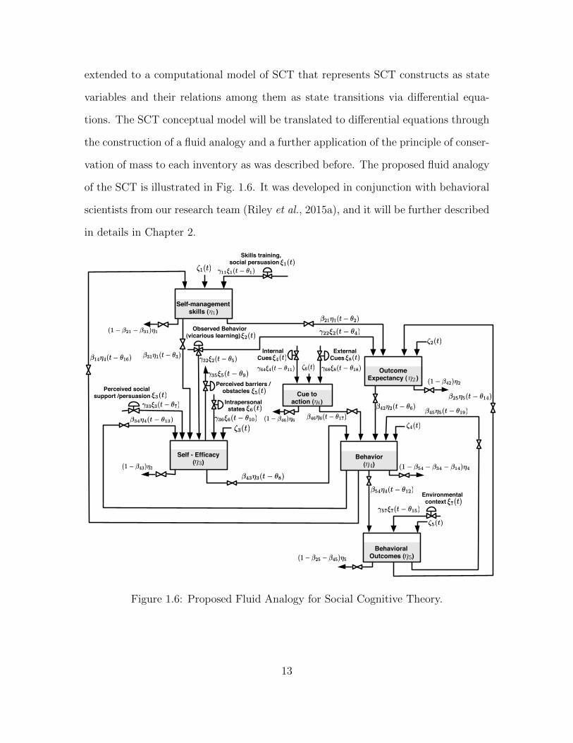
extended to a computational model of SCT that represents SCT constructs as state

variables and their relations among them as state transitions via differential equa-

tions. The SCT conceptual model will be translated to differential equations through

the construction of a fluid analogy and a further application of the principle of conser-

vation of mass to each inventory as was described before. The proposed fluid analogy

of the SCT is illustrated in Fig. 1.6. It was developed in conjunction with behavioral

scientists from our research team (Riley et al., 2015a), and it will be further described

in details in Chapter 2.

Self-management skills ( )

ζ1(t) γ11ξ1(t − θ1)ξ1(t)

Outcome Expectancy ( )

Self - Efficacy( )

Behavior( )

BehavioralOutcomes ( )

Skills training, social persuasion

Observed Behavior (vicarious learning)

(1 − β21 − β31)η1

β21η1(t − θ2)

γ22ξ2(t − θ4)ξ2(t)

Perceived social support /persuasion ξ3(t)

Perceived barriers / obstacles

Intrapersonal states ξ6(t)

ξ5(t)

γ32ξ2(t − θ5)

γ35ξ5(t − θ9)

γ36ξ6(t − θ10)

γ33ξ3(t − θ7)

γ64ξ4(t − θ11)

Environmental context

γ57ξ7(t − θ15)

ξ4(t)

ξ7(t)

ζ2(t)

ζ3(t)ζ4(t)

ζ5(t)

β31η1(t − θ3)

β42η2(t − θ6)

β54η4(t − θ12)

β25η5(t − θ14)

β34η4(t − θ13)

β43η3(t − θ8)

(1 − β54 − β34 − β14)η4

(1 − β42)η2

(1 − β43)η3

(1 − β25 − β45)η5

η1

η2

η3 η4

η5

InternalCues ξ8(t)

γ68ξ8(t − θ18)ζ6(t)

(1 − β46)η6β46η6(t − θ17)

β14η4(t − θ16)

η6

ExternalCues

Cue toaction ( )

β45η5(t − θ19)

Figure 1.6: Proposed Fluid Analogy for Social Cognitive Theory.

13

1.5.1.2 Improvements to the SCT Model

There are other well-known phenomena that can be observed in behavioral situ-

ations and are not described by SCT, such as habituation (Thompson and Spencer,

1966). This is an important feature of behavioral response resulting from continuous

stimulus. These features may be incorporated to the model as additional constructs

(i.e., inventories), relationships, or nonlinear actions. These additions to the SCT

model should be carefully studied and the decision to incorporate them must be

made based on the impact on the specific behavioral problem that is trying to be

addressed, and the increased complexity that may result from this addition.

Time (days)

0 50 100 150 200

Ste

ps

4000

5000

6000

7000

8000

9000

10000

11000

12000

13000

Daily goals

Actual steps

Figure 1.7: Hypothetical Representation of the Inverted U for a Physical Activity

Behavioral Problem Showing Step-Goals and Actual Steps.

The persistent application of a given action (e.g., incremented step-goals) may

lead to a negative response. An example for a hypothetical physical activity problem

14

is illustrated in Fig. 1.7 where daily step goals and actual steps are presented. This

type of response takes an “inverted U” form (Grant and Schwartz, 2011) and it turns

into a feature called the ideal step-goal range that is explained next. If individuals

receive step-goals that are incrementing over time, there might be a moment when

instead of incrementing their physical activity they tend to reduce it. This effect is

caused by a reduction on their perceived capability to perform the behavior caused by

a goal that they consider too ambitious to reach. Based on this effect each individual

should possess an ideal step-goal range where the goals are ambitious but doable.

Actual steps

SCT Model

Reinforcement

Step-goals

Environmental

context

Desired

behavior

(η3)Self-efficacy

Behavior(η4)

Goal

attainment

IAI

+_

Figure 1.8: Proposed Improvement to the SCT Model to Incorporate the Ideal Step-

Goal Range Feature Over the Intensively Adaptive Intervention (IAI).

One alternative to incorporate this feature to the SCT model is to introduce the

self-efficacy inventory with a signal that represents how much confidence individuals

may earn or lose, if they achieve or not the set goal for a given day. This signal is

called goal attainment, and is represented by the difference between the actual steps

and the set goal for a specific day as is depicted in Fig. 1.8. If individuals meet or

surpass the set goal on a given day, the self-efficacy level is incremented and future

behavior is reinforced; on the other hand, if the goal is not achieved self-efficacy

receives a negative effect, and the ability to reach more steps in the future is affected.

15

More details are presented in Section 2.7.2.

For validation purposes a subsection of the model will be contrasted to data from

a real physical activity intervention through the use of semi-physical identification

methods. Results will give an insight about the capability of the model to represent

behavioral situations.

1.5.2 Designing System Identification Experiments

Once the structure of the SCT dynamic model has been specified, the next step is

to design system identification experiments that are sufficiently informative to allow

the estimation of numerical values for the model parameters. Initially little infor-

mation is available about the dynamic nature of the system; hence the proposed

approach starts with the formulation of an informative experiment utilizing some of

the typical choices of input signals for system identification (e.g., Random, PRBS,

multisine, etc.). Results from the informative experiment serve as a basis for a fi-

nal experiment to find the model parameters. This experiment is formulated as an

optimization problem.

1.5.2.1 Design of an Informative Experiment

The primary goal of the informative experiment is to glean insights about the

dynamic properties of the system through the estimation of model parameters (i.e.,

gains, time constants). The experiment will be designed a priori based on previous

work focused on modeling the individual and collective impact of intervention compo-

nents on physical activity in a peer-led counseling intervention (Hekler et al., 2013a).

This approach is important because standard population-level clinical trials, while

useful for providing insights on the efficacy of an intervention package, are not suit-

able for understanding the individual dynamic response to intervention components,

16

particularly over time at an idiographic (i.e., single-subject) level.

The intervention components (i.e., inputs) at any sampling instant k are repre-

sented by u(k) and they have to be implemented under strict clinical constraints such

as high/low limits on the intervention component levels

umin ≤ u(k) ≤ umax, ∀k, (1.2)

bounded rates of change

|u(k)− u(k − 1)| ≤ b, ∀k, (1.3)

and how often the mechanism can change via a switching time (Tsw) constraint

Tsw−1∑j=1

(u(k)− u(k + j)

)= 0, ∀k = 1 + n · Tsw, n = 0, 1, 2, . . . (1.4)

The central idea is to introduce variability in data that can help capture the

inherent dynamical relationships. As this is an idiographic study design, each indi-

vidual will receive a different experimental design based on control systems methods

of pseudo randomization to support orthogonal (i.e., statistically independent) deliv-

ery of intervention components. The first intervention component goal-setting, will

be generated among a series of goals from an initial baseline behavior (e.g., 5000 daily

steps) and the target value of 10000 steps. For the second intervention component,

the focus will be on varying the amount of reinforcement points (i.e., the number of

points provided per day) available to glean insights about the appropriate amount of

points to provide for any given behavioral response.

1.5.2.2 Design of an Optimized Experiment

The primary goal of the optimized experiment is to delineate a judiciously-selected

protocol for allowing intervention features to be systematically activated and deacti-

17

vated and reactivated taking into account an improved understanding of the behavior

change process brought about by the informative experiment.

The proposed design is posed as an open-loop optimal control problem. It is as-

sumed that an a priori input-output model is known from insights from the SCT

model and informative experiment. For the purpose of illustration, it is assumed

that the interest is in modeling the dynamical relationship G between points given

for a pre-specified behavioral threshold (e.g., 10,000 steps per day) using the SCT

framework. In the proposed approach an input (daily reinforcement) sequence over

time is designed such that it reinforces behavior to reach a desired output ydes (be-

havioral threshold) which can vary over time. This is achieved by assigning points so

that the participant reaches the desired behavioral trajectory as closely as possible.

Mathematically, this can be written as:

minu∈U‖G · u− ydes‖ (1.5)

where U is defined by the set of linear inequalities (amplitude and move restriction on

input) and equalities (switching time constraint) and the objective function considers

the 2-norm of the error. The resulting optimization problem is, in general, a convex

mixed-integer quadratic program that can be efficiently solved, for most problems in

practice, using commercial solvers such as Gurobi and CPLEX.

One of the challenges of the design procedure is how to incorporate logical condi-

tions into the optimization routine to consider the deliverance of reward points based

on the attainment to the behavioral threshold. Fig. 1.9 illustrates the process through

what is called the “If/Then” block. At the beginning of the day an specific amount

of available points is offered to the patient such that at the end of the day the actual

behavior (i.e., performed steps) is compared to the set goal. If the goal was achieved

then the announced available points are granted to the individual, and they become

18

the granted reinforcement points.

Comparator X

Steps goal

Behavior

(performed steps)

Available

points

Granted

reinforcement points

1 = goal achieved0 = goal not achieved

Figure 1.9: Conceptual Representation of the “If/Then” Block That Defines the

Deliverance of Reward Points in Dependence of the Goal Attainment.

The “If/Then” block must be incorporated within the optimization procedure

that search for values of the intervention components. This will be done by defining

logic constraints through a big-M formulation (Williams, 2013) that uses the following

elements to represent such type of conditions:

• Auxiliary binary variables to represent each logic condition.

• Maximum and minimum bounds for each involved continuous variable.

• Relational operators (≤ and ≥) to represent worst case conditions using the

maximum and minimum bounds.

Another goal of the optimized experiment is to obtain input signals with less

variability according to patient-friendly definitions (Deshpande et al., 2012). This

is done inherently by the optimization procedure and via the move size constraint

described in (1.3). The performance in terms of this feature will be measured and

contrasted to results from the informative experiment.

19

1.5.2.3 Redesign of the Informative Experiment Using an Identification Test

Monitoring Approach

During the formulation of the informative experiment, the time length was consid-

ered fixed and was defined based on previous physical activity interventions. However

“patient-friendliness” concepts motivate the search for the shortest necessary dura-

tion of the experiment. This is a very important consideration in behavioral settings

where interventions can last months and resources can be consumed quickly. To

address this problem, the proposed approach uses identification test monitoring, a

concept presented by Rivera et al. (2003), with the purpose of finding the shortest

possible experimental data set with sufficient information for an adequate identifica-

tion, in terms of specific pre-defined conditions of the problem, and assuming that

noise is the main source of uncertainty in the estimation procedure.

The identification test monitoring procedure relies on the computation of statis-

tical uncertainties associated with nonparametric frequency domain estimation pro-

cedures. For a SISO system the additive uncertainty à between a real plant G and

its estimate G for each frequency ω can be defined as:

à(ω) = |G(ω)− G(ω)|, ∀ω (1.6)

Additive uncertainties can be statistically characterized to a specified probability

as is illustrated in Fig. 1.10 where confidence regions are drawn as circles of radius à

over each frequency estimate.

Deterministic and periodic input signals can be used to compute statistical uncer-

tainties in more accurate settings. Multisine signals meet the specified features and

their spectrum can be constructed by the designer in such a way the frequency grid

of interest can be directly specified. Another advantage of multisine signals is that

they allow the construction of orthogonal in-frequency signals, a feature that is very

20

ℓa(ω1)

Re{G(ω1)}

Im{G(ω1)}ℓa(ω2)

ℓa(ω3)

Figure 1.10: Representation of Statistical Confidence Regions for a Given Probability

at Each Frequency Point, Based on Additive Uncertainties for Transfer Function

Estimates G and Presented Over a Nyquist Plot.

important for the MIMO formulation. A basic specification of a multisine signal u(k)

at any sampling instant k is:

u(k) = λns∑j=1

√2αj cos(ωjkT + φj)

ωj = 2πjNsT

, k = 1, . . . , Ns

(1.7)

where Ns is the signal period, ns ≤ Ns/2 is the number of sinusoids (i.e., number of

frequencies in the grid), T is the sampling time, αj is a factor used to specify the

relative power of the jth harmonic, ωj is frequency, λ is a scaling factor, and φj is the

harmonic phase. In this dissertation, two different approaches for transfer function

and uncertainty computations are presented:

Uncertainty Computations Based on the Empirical Transfer Function Estimation

(ETFE) Method

21

Based on this representation for a SISO plant, and using the Empirical Transfer

Function Estimation (ETFE) method (Ljung, 1999) to estimate the plant model, Ba-

yard (1993) computed the following additive uncertainty with a statistical confidence

of (1− ρ)× 100%:

`2a(ω) =

2σ2|W (ω)|2αjmNs

F1−ρ(2,mNs − 2ns) (1.8)

where m is the number of cycles that the original multisine signal has been repeated,

F1−ρ(ν1, ν2) denotes the (1 − ρ) × 100 percentiles for a Fisher distribution with ν1

over ν2 degrees of freedom, W (q) is a known stable transfer function representing the

effect of output noise disturbance in the system, and σ2 is the output noise variance

estimator.

The computation of statistical uncertainties will be adjusted to consider a Multiple

Input Multiple Output (MIMO) plant, such as the one defined for the SCT model. It

also includes the definition of multisine signals that are orthogonal in-frequency using

a “zippered” power spectra design (Rivera et al., 2009) to allow the representation of

independent transfer functions for each input-output direction of the MIMO plant.

This method requires that data is considered at steady state; hence no changes on

the input signal content (e.g., amplitude or frequency content) are allowed.

Uncertainty Computations Based on the Local Polynomial Method (LPM)

The Local Polynomial Method (LPM) for periodic signals (Pintelon et al., 2011) is

utilized to incorporate some additional features that will help to present its application

in a more general setting. The included features are

• Increments on input signal amplitudes at each decision cycle with the purpose of

increase persistence of excitation while maintaining the system under operating

conditions.

22

• Frequency content adjustments on the signal period at each decision cycle. This

must be done by using harmonically related frequency grids such that the un-

certainty computation can be aggregated from one cycle to the other.

• The use of LPM enables the incorporation of the two previous features, since it

considers the transient terms for transfer function and uncertainty computation;

hence sampled data can be used without the necessity of waiting for steady state

conditions.

Relying on the LPM estimates, a 100× (1− ρ)% circular confidence region (Pintelon

and Schoukens, 2012) can be constructed as

`a(ω) =√− ln ρ σG(ω) (1.9)

where σ2G

(ω) is the sample variance of the estimated transfer function at a given

frequency ω.

According to the identification test monitoring premise, uncertainties are com-

puted at every cycle of the multisine input signal(s), and their value will influence in

the decision to halt or continue the experiment. Stopping criteria will be defined and

computed considering the following facts:

• Consideration of uncertainties in one individual transfer function element, as

well as a more general multivariable uncertainty bound that can be computed

considering maximum singular values at each frequency.

• The initial approach for computation of open-loop stopping criteria relies on

the percentage change on uncertainties from one iteration to the other; sub-

sequently, a control-related stopping criterion can also be defined relying on

robust performance ideas.

23

To evaluate the use of robust performance ideas for the monitoring procedure, the

following assumptions are made: The bound ¯a is interpreted as a scalar weight on a

normalized additive perturbation ∆a(s), where the total perturbation is LA(s)

LA(s) = ¯a ·∆a(s), σ(∆a(ω)) ≤ 1 ∀ω (1.10)

and the symbol σ(·) stands for the maximum singular value of a matrix. The block

diagram representation of the additive uncertainty of an estimated plant P within

a closed loop system is shown in Fig. 1.11, where C is a feedback controller, d′ is a

disturbance input and wP is a performance scalar weight. Under these conditions and

P

LA

∆a

+ +

+ +

ℓaI

C

wP I

d′

dy−e

_

Figure 1.11: Block Diagram of a Closed-Loop System Subject to Additive Uncertainty

LA = ¯a ·∆a.

considering a H∞ performance objective, the robust stability and robust performance

conditions (Morari and Zafiriou, 1989) are satisfied if:

σ(wP E) + σ(¯aP−1H) ≤ 1, ∀ω (1.11)

where P is the nominal plant represented by the estimated frequency response; E

and H are the sensitivity and complementary sensitivity respectively, calculated as:

E = (I + PC)−1 (1.12)

24

H = PC(I + PC)−1 (1.13)

The stopping criterion must state that the experiment can be halted if the con-

dition presented in (1.11) is satisfied for a pre-defined number of contiguous cycles.

Complete details are presented in Chapter 3.

1.5.3 Designing Closed-loop Interventions Relying on Hybrid Predictive Model

Control Ideas

The goal is to design a closed-loop Intensively Adaptive Intervention (IAI) utiliz-

ing control engineering principles, and specifically Hybrid Model Predictive Control

(HMPC) ideas to deal with the discrete natural condition of signals in behavioral

settings. The proposed approach is presented in Fig. 1.5 where the basic intervention

components are

• A goal-setting (u8) component focused on establishing the appropriate goal for

each individual (e.g., 10,000 steps).

• A daily reinforcement action (u9, u10), that represents a measure of the daily

available reward points that are under the knowledge of the participant, that are

eventually delivered to the individuals based on their behavioral achievements.

Points must have an equivalent to tangible rewards (e.g., gift cards).

In general, model predictive control is a strategy that effectively uses knowledge

of the dynamical model to predict the performance of the system over a finite time

horizon, and hence finding the best set of inputs via an optimization problem such

that the control goals (e.g., setpoint tracking, disturbance rejection) are accomplished.

The system states and outputs are computed over a prediction horizon p, while the

optimal inputs are found for a move horizon m; however the inputs are applied only

25

at the actual time. This is a receding horizon control strategy and is illustrated in

Fig. 1.12 for manipulations of step goals (u8) only. It is assumed that the measured

disturbance component (d) can be forecasted for the prediction horizon.

Prediction Horizon

Forecasted Environmental Context Report d(k+i) (if available)

Predictedsteps f

Prior steps Report (Measured Outcome)

Future Step Goals a

Prior Environmental Context Report

(Measured Disturbance)

Prior Step Goals

k k+1 k+m k+p

Move Horizon

Desired steps (Setpoint rr )

Dis

turb

.

Vari

ab

le

Co

ntr

olled

Vari

ab

le

Man

ipu

late

d

Vari

ab

le

Past Future

Time (days)

y4(k + i)

d7(k + i)

u8(k + i)umax

8

umin8

y4r(k + i)

Figure 1.12: Conceptual Representation of the Receding Horizon Control Strategy

to the Physical Activity Behavioral Problem With Control Moves Computed Only

for Step Goals (u8), and Considering Steps (y4) as the Output and Environmental

Context (d7 = ξ7) as a Measured Disturbance.

The HMPC formulation considers the simultaneous description of continuous and

discrete states and inputs. This is achieved via a mixed logical and dynamical (MLD)

structure (Bemporad and Morari, 1999). The system is represented by

x(k + 1) = Ax(k) +B1u(k) +B2δ(k) +B3z(k) +Bdd(k) (1.14)

y(k + 1) = Cx(k + 1) + d′(k + 1) + v(k + 1) (1.15)

26

E2δ(k) + E3z(k) ≤ E5 + E4y(k) + E1u(k)− Edd(k) (1.16)

where u(k), x(k), y(k), d(k), d′(k) are vectors representing the control inputs, states,

outputs, measured and unmeasured disturbances respectively, δ(k) and z(k) are aux-

iliary variables for the MLD formulation. The remaining variables are described in

Chapter 5. The optimization problem consist of finding the sequence of control ac-

tions u(k) ,.., u(k + m − 1), δ(k) ,.., δ(k + p − 1), and z(k) ,.., z(k + p − 1) that

solves

min{[u(k+i)]m−1

i=0 ,[δ(k+i)]p−1i=0 ,[z(k+i)]p−1

i=0 }

p∑i=1

‖y(k + i)− yr‖2Qy +

m−1∑i=0

‖∆u(k + i)‖2Q∆u

+m−1∑i=0

‖u(k + i)− ur‖2Qu +

p−1∑i=0

‖δ(k + i)− δr‖2Qδ

+

p−1∑i=0

‖z(k + i)− zr‖2Qz

(1.17)

subject to (1.16) and

ymin ≤ y(k + i) ≤ ymax, 1 ≤ i ≤ p (1.18)

umin ≤ u(k + i) ≤ umax, 0 ≤ i ≤ m− 1 (1.19)

∆umin ≤ ∆u(k + i) ≤ ∆umax, 0 ≤ i ≤ m− 1 (1.20)

where yr, ur, δr, and zr are the referential (i.e., desired) values for each respective

signal.

One objective of the closed-loop IAI is to ensure that individuals maintain their

levels of physical activity even after the initial, and more aggressive, part of the

intervention has been completed. The idea is to keep monitoring the performance of

participants to detect when they have reached the required levels of behavior for a

predefined time interval. If that is the case, the system can be moved to a second

maintenance phase where reward points can be partially or completely removed such

that individuals continue following step goals based on their achieved self-efficacy

levels. This can be implemented over the HMPC approach by reconfiguring the

27

weight matrices (Qu) for the required inputs, in the optimization problem presented

in (1.17). A detailed formulation of the problem is presented in Chapter 5.

1.6 Contributions of the Dissertation

This dissertation presents a framework for the design of effective intensively adap-

tive interventions based on control systems principles for low physical activity be-

havioral problems. The development definition of identification test monitoring is

consequently described. Different research activities have been developed in several

stages, covering important aspects of design procedures.

The contributions of this work in terms of modeling behavioral theories can be

summarized as follows:

• Development of a novel dynamical systems model for Social Cognitive Theory

(SCT), relying on fluid analogies to represent the relations among different

constructs as are described in narrative form by the theory. The modeling

study includes the definition of operational and stability conditions.

• Enhancement of the model by incorporating habituation, a nonlinear phe-

nomenon. This is performed via a parameter varying technique using a gain

scheduling approach.

• Application of semiphysical system identification routines to find values for

parameters according to the SCT model, for a given noise set of input-output

data.

• Incorporation of model improvements motivated by the physical activity prob-

lem. In particular, understanding the ideal step-goal range of individuals,

achieved by linking the effect of goal attainment to self-efficacy.

28

The contributions of this dissertation in terms of designing system identification

experiments in an open-loop intensively adaptive behavioral intervention are

• Development of an open-loop system identification experiment using random

yet bounded input signals.

• Development of a novel MIMO identification test monitoring procedure to find

the shortest possible experiment with sufficient information for identification

purposes. This approach relies on the computation of frequency domain transfer

function estimates, yielding to the definition of additive uncertainty bounds that

are used in the formalization of stopping criteria that enable the decision to halt

or continue the experiment.

• Development of an enhanced identification test monitoring procedure incor-

porating transient responses in the computation of transfer functions and un-

certainties, such that additional input signal modifications can be considered.

These additional modifications over the input signals are: amplitude modifica-

tions, and changes on the harmonic frequency content.

• Formulation of more general stopping criteria for MIMO identification test mon-

itoring. These criteria rely on the application of robust control ideas over a

closed-loop representation.

• Development of a novel optimized system identification experiment utilizing

initial results from the informative experiment. This experiment is formulated

as an optimization problem where the objective is to track a desired output

behavior profile, relying on the informative model, and under operational and

economic constraints.

29

In terms of designing a long term closed-loop Intensively Adaptive Intervention

(IAI) for the physical activity behavioral problem, the contributions of this disserta-

tion are

• Development of an intervention algorithm relying on Hybrid Model Predictive

Control (HMPC) framework that is able to personalize the discrete level of

interventions components, reaching the objectives of setpoint tracking, and dis-

turbance rejection.

• Extension of the mixed logical dynamical (MLD) structure to allow the formu-

lation of structures that are specific to the behavioral problem. This was used

to represent the effect of the If/Then block that allows the deliverance of reward

points when the set goal has been achieved.

• Development of a reconfiguration strategy of HMPC parameters to allow the

introduction of the maintenance stage, where rewards might be reduced based

on the incremented capacity of individuals to reach the set goal. This is done by

reconfiguring the weight matrices used in the objective function for optimiza-

tion.

1.7 Dissertation Outline

Following this introduction, the dissertation continues with Chapter 2 that presents

the detailed formulation of the dynamical systems model for SCT. The chapter shows

how the fluid analogy is developed, including the definition of a system of differen-

tial equations that represents the model. Model enhancements are also presented,

incorporating two important behavioral features: habituation and ideal range for

step-goals. The semiphysical identification procedure is presented and the model is

validated via simulation of representative cases and reconciliation to a data set from

30

an actual physical activity intervention.

In Chapter 3 the general multivariable identification test monitoring procedure

is presented. A frequency domain approach for computing transfer functions and

uncertainties is developed. Two different alternatives are proposed: the first relies on

Empirical Transfer Function Estimates (ETFE) utilizing sampled data measured at

steady state. The second approach uses the Local Polynomial Method (LPM), which

includes the effects of transient responses, such that additional modifications in the

inputs are allowed. A general stopping criterion is also developed relying on robust

control ideas. Finally a simulation study is presented using as a reference, a process

control plant model.

Chapter 4 describes how open-loop behavioral intensively adaptive interventions

are developed for system identification purposes. The design of the informative and

optimized experiments is detailed. For the informative experiment two different ap-

proaches are presented: the first one using random generated input signals under

operational constraints; the second one uses multisine input signals with frequency

content specifically designed to excite frequencies of interest. The two different iden-

tification test monitoring approaches are applied (i.e., utilizing ETFE or LPM), and a

complete simulation study representing a hypothetical low physical activity problem

is presented.

Chapter 5 presents the design of closed-loop intensively adaptive behavioral in-

terventions with the purpose to reach and sustain the required amount of physical

activity. The design procedure relies on Hybrid Model Predictive Control (HMPC)

ideas that allow the simultaneous use of discrete and continues values for inputs and

states. The chapter describes how the HMPC algorithm is adapted and improved

to represent the discrete nature of the behavioral intervention components and some

of the logical blocks of the model. Some of the HMPC parameters are reconfigured

31

during experimental execution to allow the initiation of a maintenance stage where

behavior is sustained mainly by the improved capacity of individuals earned in the

early stages of the intervention. During this phase, rewards can be partially removed.

Finally the dissertation concludes in Chapter 6 with a summary and conclusions of

the major contributions of this work. The chapter includes directions and suggestions

for future work.

1.8 Publications

The material presented in this dissertation has been taken primarily from a se-

ries of published and submitted papers with the following detail: The material for

Chapter 2 has been taken from:

1. C. A. Martın, D. E. Rivera, W.T. Riley, E. B. Hekler, M. P. Buman, M. A.

Adams and A. C. King. A dynamical systems model of Social Cognitive Theory.

In Proceedings of the 2014 American Control Conference (ACC), pages 2407-

2412, July 2014. (Martın et al., 2014).

2. W.T. Riley, C. A. Martın, D. E. Rivera, E. B. Hekler, M. A. Adams, M. P.

Buman, M. Pavel and A. C. King. Development of a dynamical systems model

of Social Cognitive Theory. In Translational Behavioral Medicine: Practice,

Policy and Research, pages 1 - 13, November 2015, doi = 10.1007/s13142-015-

0356-6. (Riley et al., 2015a).

Contents from this chapter have been partially adapted into the following papers:

3. W.T. Riley, C. A. Martın, and D. E. Rivera. The importance of behavior theory

in control system modeling of physical activity sensor data. In Proceedings of

the 2014 36th Annual International Conference of the IEEE Engineering in

32

Medicine and Biology Society, pages 6880 - 6883, August 2014. (Riley et al.,

2014).

4. K. P. Timms, C. A. Martın, D. E. Rivera, W.T. Riley, and E. B. Hekler. Lever-

aging intensive longitudinal data to better understand health behaviors. In

Proceedings of the 2014 36th Annual International Conference of the IEEE En-

gineering in Medicine and Biology Society, pages 6888 - 6891, August 2014.

(Timms et al., 2014a).

5. E. B. Hekler, P. Klasnja, W. T. Riley, M. P. Buman, J. Huberty, D. E. Rivera,

and C. A. Martın. Agile science: creating useful products for behavior change

in the real world. In Translational Behavioral Medicine, volume 6, issue 2, pages

317 - 328, 2016. (Hekler et al., 2016).

The material from Chapter 3 has been adapted from:

6. C. A. Martın, D. E. Rivera, and E.B. Hekler. An identification test monitoring

procedure for MIMO systems based on statistical uncertainty estimation. In

Proceedings of the 54th Conference on Decision and Control (CDC) 2015, pages

2719 - 2724, December 2015. (Martın et al., 2015c).

7. C. A. Martın, D. E. Rivera, and E.B. Hekler. An enhanced identification test

monitoring procedure for MIMO systems relying on uncertainty estimates. Sub-

mitted to the 55th Conference on Decision and Control (CDC) 2016. (Martın

et al., 2016b).

Contents of Chapter 4 have been adapted from:

8. C. A. Martın, S. Deshpande, E.B. Hekler, and D. E. Rivera. A system identifica-

tion approach for improving behavioral interventions based on Social Cognitive

33

Theory. In Proceedings of the 2015 American Control Conference, pages 5878 -

5883, July 2015. (Martın et al., 2015a).

9. C. A. Martın, D. E. Rivera, and E.B. Hekler. Design of informative identifica-

tion experiments for behavioral interventions. In Proceedings of the 17th IFAC

Symposium on System Identification, SYSID 2015, pages 1325 - 1330, October

2015. (Martın et al., 2015b).

Finally, the material presented in Chapter 5 is described in:

10. C. A. Martın, D. E. Rivera, and E.B. Hekler. A decision framework for an adap-

tive behavioral intervention for physical activity using hybrid model predictive

control. In Proceedings of the 2016 American Control Conference, pages 3576 -

3581, July 2016. (Martın et al., 2016a).

The following publications are submitted or under preparation:

1. C. A. Martın, D. E. Rivera, W.T. Riley, E. B. Hekler, M. P. Buman, M. A.

Adams, and A. Magann. Development of a dynamical model of Social Cogni-

tive Theory for adaptive behavioral interventions. To be submitted to IEEE

Transactions on Control Systems Technology.

2. D. E. Rivera, C. A. Martın, K. P. Timms, S. Deshpande, N.N. Nandola, and

E.B. Hekler. Control systems engineering for optimizing behavioral mHealth

interventions. In S. Murphy, J. Rehg, and S. Kumar (Eds.) Mobile health:

sensors, analytic methods, and applications, 2016.

3. C. A. Martın, D. E. Rivera, and E.B. Hekler. A control engineering approach

for optimizing physical activity behavioral interventions. Submitted to IEEE

Ecuador Technical Chapters Meeting (ETCM), 2016.

34

4. E.B. Hekler, D.E. Rivera, C.A. Martin, P. Klasnja, W.T. Riley, M.P. Buman,

M. Adams, S. Phatak, E. Korinek, and M. Freigoun. Control-System Driven In-

tensively Adaptive Interventions: A Detailed Account on how Control Systems

Engineering Can be Used to Advance Behavioral Science Theory and Practice.

5. E. Korinek, S. Phatak, D.E. Rivera, C.A. Martin, M. Freigoun, and E.B. Hek-

ler. EAdaptive Step Goals: A longitudinal growth model of daily steps for a

smartphone-based walking intervention.

6. S. Phatak, E. Korinek, D.E. Rivera, C.A. Martin, M. Freigoun, and E.B. Hekler.

A System Identification Validation Study of a Dynamical Model Version of

Social Cognitive Theory.

The following are additional journal publications that are anticipated from this

dissertation:

1. C. A. Martın, D. E. Rivera, and E.B. Hekler. A MIMO approach for the

formulation of identification test monitoring experiments relying in robust per-

formance ideas.

2. C. A. Martın, D. E. Rivera, and E.B. Hekler. Designing informative and opti-

mized system identification experiments for open-loop physical activity behav-

ioral interventions.

3. C. A. Martın, D. E. Rivera, and E.B. Hekler. Decision policies for closed-loop

physical activity behavioral interventions relying on a HMPC formulation.

35

Chapter 2

MODELING BEHAVIORAL INTERVENTIONS USING SOCIAL COGNITIVE

THEORY

2.1 Overview

Behavioral theories play a central role in the creation of behavior change strate-

gies and thus their choice within a specific problem is important. Social Cognitive

Theory (SCT) has been used as the basis for many behavioral interventions (Lopez

et al., 2011); it provides a conceptual framework of the theorized influences on be-

havior and their interdependences that is amenable to various modeling techniques.

Robust computational modeling approaches can provide a flexible and rigorous test

to confirm, revise, or refute SCT and other theories (Nilsen and Pavel, 2013). Further

computational models can aid in better specifying contextually relevant and instanta-

neous interrelationships measured continuously via mobile and wireless technologies.

In a recent review of mobile health interventions, SCT or one of its variants served as

the basis for all smoking cessation interventions that reported a theoretical basis and

was the predominant theoretical basis for weight management interventions reviewed

(Riley et al., 2011).

While not specified in SCT, external stimuli are shown to affect behavior according

to the principles of behavioral response habituation (Thompson and Spencer, 1966),

including: decreased responses following repeated application of stimuli, recovery of

responses when stimuli are withheld, and reduction of responses with increased stim-

ulation frequency. To then illustrate that the effectiveness of an increasing positive

stimulus in humans is often nonmonotonic, an “inverted U” phenomenon (Grant and

36

Schwartz, 2011) has been incorporated into the linear SCT model. For the case of low

physical activity, this feature is expressed as an ideal range of step goals dependent

on the current level of training and predisposition to walk of individuals.

In this chapter, a dynamical systems model for SCT is proposed based on its

constructs and interrelationships (Bandura, 1986). Simulations of the model using

physical activity of individuals over time as a referential behavior are performed.

The model features a nonlinear structure that addresses habituation, and some linear

modifications to represent the ideal range of step goals. Through a semi-physical

identification procedure, a subsection of the model is reconciled to actual data from

MILES, a lifestyle intervention involving mobile technology. A model like the one

proposed in this paper can ultimately serve as the controller model in an intensively

adaptive intervention using MPC (Riley et al., 2015b; Nandola and Rivera, 2013).

The chapter is organized as follows: Section 2.2 presents a brief description of

SCT and its core elements. Section 2.3 describes the development of the fluid anal-

ogy based on the interconnections between the constructs and components of SCT.

Section 2.4 presents how the model was constructed including mathematical details,

assumptions and how habituation is represented. Section 2.5 discusses simulation re-

sults for a hypothetical case study. Section 2.6 contrasts experimental data obtained

from a physical activity intervention against simulations using the model. Section 2.7

presents model improvements that can be applied specifically to a physical activity

intervention.

2.2 Social Cognitive Theory

Social Cognitive Theory (SCT) has its basis in early learning theory, which does

not account for behaviors learned by means other than prior experience. This led to

the seminal work of Bandura (Bandura and Walters, 1963) on Social Learning Theory

37

(SLT), which incorporated the principles of observational or vicarious learning. SLT,

however, failed to incorporate the self-belief and perceptions of the individual, leading

to the introduction of the concept of self-efficacy (Bandura, 1977).

SCT describes a human agency model in which individuals proactively self-reflect,

self-regulate, and self-organize (Bandura, 1989). Core to this perspective is the con-

cept of reciprocal determinism or triadic reciprocity depicted in Fig. 2.1 in which

personal influences (cognitions, affect, biology) and environment interact and mutu-

ally shape one another. Both of these factors interact and influence behavior, and

that behavior, in turn, reciprocally shapes personal and environmental factors.

Behavior

Person Environment

Figure 2.1: Triadic Reciprocal Determinism of Social Cognitive Theory.

In essence, SCT estimates the ability of an individual to engage in a determined

behavior based on internal and external parameters and their interrelationships. Some

of these are self-perceived and others can be externally measured.

The following SCT components are generated as a consequence of the variation

of external or internal stimuli, considered outputs from an engineering point of view.

These components are:

• Self-efficacy, the perceived capability to do what is required to perform a given

behavior. It plays a core role as a personal factor that influences behavior. It

is influenced by behavior and the environment.

• Outcome expectancies, the perceived likelihood that performing a given behavior

38

will result in certain outcomes. It is also a central component of the personal

factors that influence behavior and are influenced by environment and behavior.

• Behavioral outcomes, the outcomes obtained as a result of engagement in the

behavior of interest. These are directly related to outcome expectancies and

the future behavior.

• Self-management skills, the set of skills involving a class of complex behaviors

such as self-monitoring, goal setting, self-reinforcement, stimulus control, and

related methods by which an individual increases the potential success for a

given behavior. These contribute directly to self-efficacy.

• Behavior, the actual behavior studied, which can correspond to a particular

metric of physical activity (e.g., number of daily steps taken, minutes spent in

daily moderate-to-vigorous physical activity) or to involvement with an addic-

tive substance (e.g., the number of cigarettes or alcoholic drinks consumed in a

given day).

According to the theory, there are variables that act as stimuli to promote or

discourage behavior and the previous components. These are considered inputs, and

can be external or internal to the individual. They are:

• Skills training. These activities help to increase (or decrease) the self-management

skills of the individual. An example for physical activity is learning to use a

pedometer.

• Observed behavior (vicarious learning). This influences not only self-efficacy

for engaging in the behavior, but also outcome expectancies as the individual

observes results of others performing the behavior.

39

• Perceived social support and verbal persuasion. These can help to increase self-

efficacy. An example is the availability of others to engage in physical activity

with the individual or to verbally support increased physical activity of the

individual.

• Perceived barriers and obstacles. These are external conditions that affect be-

havior. For example, physical activity can be reduced because of insufficient

time, bad weather, and limited access to exercise facilities or safe walking paths.

• Intrapersonal states. These consist of an array of physical, mental, and emo-

tional states of the individual, such as happiness and sadness, that either in-

crease or decrease self-efficacy at any given time.

• Environmental context. This influences directly the resultant behavioral out-

comes.

• Internal and external cues. These directly influence behavior. In SCT, self-

efficacy and outcome expectancies are often conceptualized as predispositions

for engaging in any given behavior that is then triggered by a cue to action.

In a more granular model, cue to action is likely to be treated as discrete and

episodic inputs.

2.3 Developing a Fluid Analogy for SCT

The proposed fluid analogy of Social Cognitive Theory (SCT) is presented in

Fig. 2.2. It depicts how the various components of SCT relate with one another

over time, particularly to understand behavior. The use of a fluid analogy allows the

organization of behavioral ideas into a structured framework that can be used to find

a mathematical model. Main constructs are treated as inventories; other components

40

Self-management skills ( )

ζ1(t) γ11ξ1(t − θ1)ξ1(t)

Outcome Expectancy ( )

Self - Efficacy( )

Behavior( )

BehavioralOutcomes ( )


Observed Behavior (vicarious learning)

(1 − β21 − β31)η1

β21η1(t − θ2)

γ22ξ2(t − θ4)ξ2(t)

Perceived social support /persuasion ξ3(t)


Intrapersonal states ξ6(t)

ξ5(t)

γ32ξ2(t − θ5)

γ35ξ5(t − θ9)

γ36ξ6(t − θ10)

γ33ξ3(t − θ7)

γ64ξ4(t − θ11)


γ57ξ7(t − θ15)

ξ4(t)

ξ7(t)

ζ2(t)

ζ3(t)ζ4(t)

ζ5(t)

β31η1(t − θ3)

β42η2(t − θ6)

β54η4(t − θ12)

β25η5(t − θ14)

β34η4(t − θ13)

β43η3(t − θ8)(1 − β54 − β34 − β14)η4

(1 − β42)η2

(1 − β43)η3

(1 − β25 − β45)η5

η1

η2

η3 η4

η5

InternalCues ξ8(t)

γ68ξ8(t − θ18)ζ6(t)

(1 − β46)η6β46η6(t − θ17)

β14η4(t − θ16)

η6

ExternalCues

Hab

LTCue to

action ( )

β45η5(t − θ19)

Figure 2.2: Fluid Analogy for Social Cognitive Theory, Augmented With Habituation.

and properties are depicted as inflows and/or outflows.

In the schematic, behavior (η4) is represented as a fluid inventory that changes

in frequency and/or duration over time based on various putative SCT factors. This

model was developed based on a daily time frame (i.e., aggregate frequency and/or

duration of behavior within any given day). Similar models with more or less granular

time frames could be adapted from this daily time frame depending on the behavior

of interest (e.g., smoking or cancer screening behaviors) and time frame of interest.

Self-efficacy (SE) (η3) is a core construct of SCT and is represented as an inven-

tory of varying levels that differs not only between individuals and specific behaviors,

41

but also fluctuates within an individual over time. SE functions as both an indepen-

dent variable influencing the likelihood of engaging in the associated behavior, and

a dependent variable influenced by a number of factors that increase or decrease the

inventory at any given time. The following are the SCT factors that are theorized to

increase or decrease the SE inventory:

1. Perceived barriers and obstacles (ξ5) to engaging in any given behavior deplete

self-efficacy (SE).

2. Perceived social support and verbal persuasion from others increases SE (ξ3).

3. Observed behavior (vicarious learning) (ξ2) of others successfully performing the

behavior increases SE.

4. Intra-personal states of the individual (ξ6) either add to or deplete the level of

SE.

5. Prior experience engaging in the behavior (β34) is a gain parameter representing

the critical learning feedback loop that adds or depletes SE to subsequently

engage in the behavior. This is a feedback loop in which successfully engaging

in the behavior increases SE to engage in the behavior, which subsequently

increases the likelihood of engaging in the behavior.

6. Self-management or self-regulatory skills (η1) influence both SE and outcome

expectancies. Inputs into the self-management inventory include formal skills

training, observational learning, and verbal persuasion (ξ1).

The inventory outcome expectancies (η2) is another important construct in SCT

that contributes to the likelihood of any given behavior. These behaviors are inher-

ently followed by positive and/or negative consequences, some proximal and some

42

distal, or lack of consequences. For example, engaging in physical activity could re-

sult, short term, in feeling fatigued or invigorated. Social reinforcement may ensue

from engaging in physical activity. Over the longer-term, physical activity may lead

to improved health, or conversely in injury. These behavioral outcomes (η5) produce a

feedback loop to outcome expectancies (β25). Experiencing and/or expecting positive

outcomes from engaging in the behavior will lead to an increased likelihood of subse-

quently engaging in the behavior. As previously noted, these behavioral outcomes are

greatly influenced by the environmental context in which the behavior occurs (ξ7).

The second input into outcome expectancies is observational learning or modeling

(ξ2). Observing the consequences of the behavior experienced by others adds or

depletes the outcome expectancy inventory for that behavior. The third component

that influences outcome expectancies is self-regulatory or self-management skills (β21).

Finally, cue to action (η6) directly influences behavior and is treated as an inven-

tory that represents the various cues to action that occur during the day. These cues

can be external (e.g., friend asks to take a walk) or internal (e.g., getting tired or

stiff from sitting). They can occur naturally (e.g., good weather) or artificially (e.g.,

alarm reminder on phone to go for a walk) in the environment. To complete the fluid

analogy model, disturbances (ζ) are added. Disturbances are any exogenous factors

that influence the inventories and can be viewed as unexplained variance.

Path diagrams are part of Structured Equation Modeling (SEM; Bollen (1989)).

They are used to depict the associations among a set of variables that later can be

represented in the form of linear equations. In this case, a reverse process is developed.

The path diagram for Social Cognitive Theory shown in Fig. 2.3, is obtained from

the connections established in the proposed fluid analogy.

43

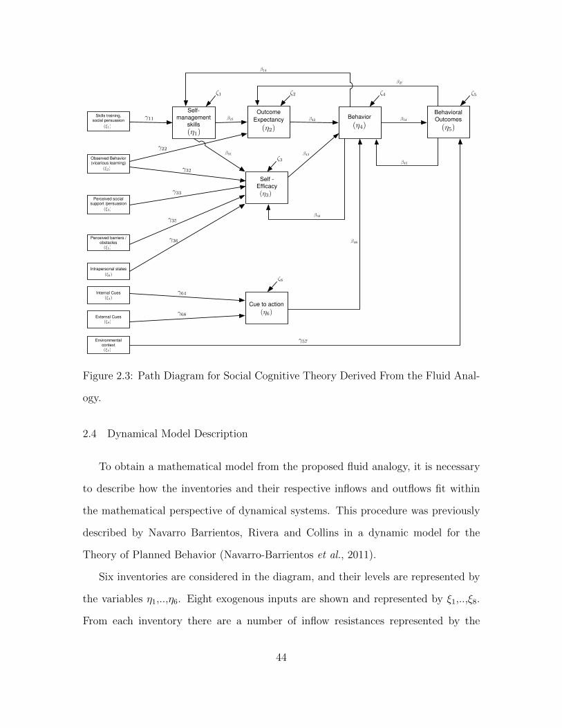
Self-

management

skills

Outcome

Expectancy

Self -

Efficacy

(η3)

(η1)(η2)

Behavior

(η4)

Behavioral

Outcomes (η5)


(ξ1)

Observed Behavior(vicarious learning)

Perceived social support /persuasion

External Cues


Intrapersonal states


(ξ2)

(ξ3)

(ξ8)

(ξ5)

(ξ6)

(ξ7)

γ11

γ22

γ32

γ33

γ64

γ35

γ36

γ57

β21

β31

β42

β43

β54

β34

β25

ζ1 ζ2 ζ4

ζ3

ζ5

Cue to action

(η6)

β14

Internal Cues(ξ4)

β46

γ68

ζ6

β45

Figure 2.3: Path Diagram for Social Cognitive Theory Derived From the Fluid Anal-

ogy.

2.4 Dynamical Model Description

To obtain a mathematical model from the proposed fluid analogy, it is necessary

to describe how the inventories and their respective inflows and outflows fit within

the mathematical perspective of dynamical systems. This procedure was previously

described by Navarro Barrientos, Rivera and Collins in a dynamic model for the

Theory of Planned Behavior (Navarro-Barrientos et al., 2011).

Six inventories are considered in the diagram, and their levels are represented by

the variables η1,..,η6. Eight exogenous inputs are shown and represented by ξ1,..,ξ8.

From each inventory there are a number of inflow resistances represented by the

44

coefficients γ11,..,γ68 and outflow resistances represented by β21,..,β54. One approach

to conceptualize these resistances is to consider those as the fraction of each inventory

or input that leaves the previous instance and then feeds the next inventory.

There are other parameters that represent the physical characteristics of each in-

ventory and flow; these have an important effect on the dynamic behavior of the

system. First time constants τ1,..,τ6 represent the capacity and allow for exponential

decay (or growth) of the inventory. Time delays (θ1,..,θ19) for each flow signal are also

used. Finally unmeasured disturbances (which may reflect unmodeled dynamics) are

considered as ζ1,..,ζ6.

2.4.1 Differential Equation Representation

After the application of the fluid analogy the behavioral variables are treated as

physical entities. The principle of mass conservation is used: the sum of the inflows

minus the outflows gives an accumulation term denoted by the time constant τ times

the rate of change in the level of the inventory. The sum of all outflows must add up

to the value of the respective inventory. For that reason, at each inventory output,

an outflow of (1− βjk − ...− βlm)ηi(t) is included in the model, where the β’s are the

respective outflow coefficients.

To demonstrate how the equations are derived, a subsection of the fluid analogy

including only the first inventory (Self-management Skills (η1)) with its inflows and

outflows is presented in Fig. 2.4.

The principle of mass conservation applied to η1 is

τ1dη1

dt=γ11ξ1(t− θ1) + β14η4(t− θ16) + ζ1(t)− β31η1(t)− β21η1(t)

− (1− β21 − β31)η1(t)

(2.1)

45

Self-management skills

ζ1(t)γ11ξ1(t − θ1)

ξ1(t)

(1 − β21 − β31)η1 β21η1(t)β31η1(t)

(η1)

β14η4(t − θ16)


From η4

To

To

η3

η2

Figure 2.4: Self-Management Skills Inventory (η1) Showing All its Inflows and Out-

flows

which following simplifications yields

τ1dη1

dt= γ11ξ1(t− θ1) + β14η4(t− θ16)− η1(t) + ζ1(t) (2.2)

Applying the same procedure for all the inventories, the following system of dif-

ferential equations is obtained:

τ2dη2

dt= γ22ξ2(t− θ4) + β21η1(t− θ2) + β25η5(t− θ14)− η2(t) + ζ2(t) (2.3)

τ3dη3

dt=γ32ξ2(t− θ5) + γ33ξ3(t− θ7)− γ35ξ5(t− θ9) + γ36ξ6(t− θ10)

+ β31η1(t− θ3) + β34η4(t− θ13)− η3(t) + ζ3(t)

(2.4)

τ4dη4

dt=β42η2(t− θ6) + β43η3(t− θ8) + β46η6(t− θ17) + β45η5(t− θ19)

− η4(t) + ζ4(t)

(2.5)

τ5dη5

dt= γ57ξ7(t− θ15) + β54η4(t− θ12)− η5(t) + ζ5(t) (2.6)

τ6dη6

dt= γ64ξ4(t− θ11) + γ68ξ8(t− θ18)− η6(t) + ζ6(t) (2.7)

The model per (2.2)–(2.7) consists of a system of first-order differential equations,

46

but to describe a more elaborate transient response (such as overdamped, critically

damped or underdamped responses), a second order system could be used (Navarro-

Barrientos et al., 2011). If second order dynamics are present, these can be concep-

tualized as being part of an inventory system that is subject to self-regulation. This

will be illustrated with an example considering only one inventory as a reference: to

represent cue to action (η6) as a system with one zero and two poles and assuming

for simplicity that the input ξ4 (internal cue) is equal to zero, the equation (2.7) can

be rewritten as

τ 26

d2η6

dt2+ 2ζτ6

dη6

dt=γ68

(ξ8(t− θ18) + τa

dξ8(t− θ18)

dt

)− η6(t) + ζ6(t) (2.8)

that, after neglecting delays and perturbations, yields to the transfer function:

η6(s)

ξ8(s)=

γ68(τas+ 1)

τ 26 s

2 + 2ζτ6s+ 1(2.9)

To depict this second order system within the fluid analogy, a self-regulatory

controller for each inventory should be included. To illustrate this process, in Fig. 2.5

the inventory cue to action (η6) is shown with its inflows and outflows, excluding ξ4.

ξ8(t)γ68ξ8(t − θ18)

ζ6(t)

(1 − β46)η6 β46η6(t − θ17)

η6

External

Cues

ControllerC

LT

Cue toaction ( )

Figure 2.5: Inventory Cue to Action (η6) With the Addition of a Feedback Controller

to Represent a Second Order System.

To obtain a more general representation, in concordance with control systems

47

literature, the following variables are substituted:

d = ξ8; y = η6; τ = τ6; K = γ68

yielding the following transfer function:

y(s)

d(s)=

K(τas+ 1)

τ 2s2 + 2ζτs+ 1(2.10)

Fig. 2.6 represents a block diagram for a general second order inventory system with

the proposed variables, where τp is the first order time constant for the tank.

1τps+1

Kτps+1

++

+

-

c(s)

d(s)

y(s)r(s)p

pd

Figure 2.6: Block Diagram for a Second Order Inventory System.

The controller c(s) must be selected such that the transfer function from d(s) to

y(s) matches the required second order system. To obtain a mathematical representa-

tion of the controller, a reverse engineering procedure is performed using the Internal

Model Controller (IMC) design method (Morari and Zafiriou, 1989), applied to the

following first order plant model:

p =1

τps+ 1(2.11)

From here the initial q-parametrized controller, and the obtained filter are

q = τps+ 1, f =λs

(λ1s+ 1)(λ2s+ 1)(2.12)

48

resulting in

q =λs(τps+ 1)

(λ1s+ 1)(λ2s+ 1)(2.13)

The required transfer function can be represented in terms of the IMC controller as

y

d= (1− pq)pd =

(1− λs

(λ1s+ 1)(λ2s+ 1)

) K

τps+ 1(2.14)

After some mathematical simplifications the result from (2.14) is compared to (2.10),

from where the following relations are obtained:

λ1λ2 = τ 2 = τpτa (2.15)

λ1 + λ2 = 2ζτ (2.16)

λ = τp + τa − 2ζτ (2.17)

and the values for the filter coefficients (λi) can be derived. To avoid a neglected

controller the following condition must be satisfied:

λ1 + λ2 6= τp + τa (2.18)

Using these representations, the transfer function c(s) can be represented in a classical

feedback controller form as

c(s) =(2ζτ − τa − τp)s

τas+ 1(2.19)

The presence of a feedback controller creates a connection to another behavioral

theory, self-regulation (Carver and Scheier, 1998).

2.4.2 Model Considerations

The following model assumptions are considered to enforce the mass conservation

principle and for simulation purposes:

49

• The time unit is in days.

• The β coefficients must satisfy the following constraints to enforce that the sum

of outflows must add up to the value of the respective inventory:

β21 + β31 ≤ 1, β42 ≤ 1, β43 ≤ 1

β54 + β34 + β14 ≤ 1, β25 + β45 ≤ 1, β46 ≤ 1

• The initial levels of the inventories are determined by solving the system of

equations at steady state, obtaining the following results:

η1 = γ11ξ1 + β14η4

η2 = A+ (β21β14 + β25β54)η4

η3 = B + (β31β14 + β34)η4

η4 =β46η6 + β42A+ β43B + β45γ57ξ7

1− β42(β21β14 + β25β54)− β43(β31β14 + β34)− β45β54

η5 = γ57ξ7 + β54η4

η6 = γ64ξ4 + γ68ξ8

where

A = γ22ξ2 + β21γ11ξ1 + β25γ57ξ7

B = γ32ξ2 + γ33ξ3 − γ35ξ5 + γ36ξ6 + β31γ11ξ1

• All inventories are restricted to have values within 0 and 100 %.

• Uncertainties are represented as zero mean stochastic signals.

• The exogenous signals: intrapersonal states (ξ6) and environmental context (ξ7)

are considered as auto-correlated noise since they may occur in a nearly random

way.

All time delays are considered to be zero; this is for simplicity and clarity of results.

50

2.4.3 Stability Analysis

Using the state space representation of the system based on the SCT model, the

state matrix is

A =

− 1τ1

0 0 β14

τ10 0

β21

τ2− 1τ2

0 0 β25

τ20

β31

τ30 − 1

τ3

β34

τ30 0

0 β42

τ4

β43

τ4− 1τ4

β45

τ4

β46

τ4

0 0 0 β54

τ5− 1τ5

0

0 0 0 0 0 − 1τ6

(2.20)

The system is stable if all the eigenvalues of A have negative real parts. To verify

this condition the characteristic equation of the matrix A is computed as

D(s) = |sI−A| = a5s5 + a4s

4 + a3s3 + a2s

2 + a1s+ a0 (2.21)

with:

a5 = τ1τ2τ3τ4τ5 (2.22)

a4 = τ1τ2τ3τ4 + τ1τ2τ3τ5 + τ1τ2τ4τ5 + τ1τ3τ4τ5 + τ2τ3τ4τ5 (2.23)

a3 =τ1τ2τ5(1− β34β43) + τ1τ2τ3(1− β45β54) + τ1τ2τ4 + τ1τ3τ4 + τ1τ3τ5

+ τ2τ3τ4 + τ1τ4τ5 + τ2τ3τ5 + τ2τ4τ5 + τ3τ4τ5

(2.24)

a2 =τ1τ5(1− β34β43) + τ1τ2(1− β34β43 − β45β54)

+ τ2τ5(1− β34β43 − β14β31β43) + τ1τ3(1− β45β54 − β25β42β54)

+ τ2τ3(1− β45β54) + τ3τ5(1− β14β21β42) + τ1τ4

+ τ2τ4 + τ3τ4 + τ4τ5

(2.25)

51

a1 =τ1(1− β34β43 − β45β54 − β25β42β54)

+ τ2(1− β34β43 − β45β54 − β14β31β43)

+ τ3(1− β45β54 − β14β21β42 − β25β42β54) + τ4

+ τ5(1− β34β43 − β14β21β42 − β14β31β43)

(2.26)

a0 = 1− β34β43 − β45β54 − β14β21β42 − β14β31β43 − β25β42β54 (2.27)

The stability condition is satisfied if all of the coefficients of D(s) are positive, there-

fore the set of conditions for stability is

ai > 0, i = 0, · · · , 5 (2.28)

Considering that all time constants τj are positive, the only possibility for any term

ai to be negative is if one or more of its internal factors 1 − (βiβj) − · · · − (βkβlβm)

are negative. To prevent this for any specific internal factor, the following condition

must be met:

(βiβj) + · · ·+ (βkβlβm) < 1 (2.29)

One general way to meet this requirement is to consider that each gain β is less than

one, therefore to have a stable system it is sufficient that all of the following conditions

are met simultaneously:

β21 < 1, β31 < 1, β42 < 1, β43 < 1, β54 < 1, β34 < 1, β14 < 1, β25 < 1, β45 < 1 (2.30)

2.4.4 Nonlinear Dynamics of Habituation Within the SCT Model

It was noted previously that human behavior is a complex process. Even when

is described by elaborate theories such as SCT, it can change its direction based on

particular scenarios; one of these is habituation. Habituation is a behavioral phe-

nomenon that is triggered by repeated stimulation. It results in decreased responses

52

despite increased stimulus. It does not involve sensory adaptation, sensory fatigue, or

motor fatigue (Rankin et al., 2009); the decrease usually follows a negative exponen-

tial curve. Marsland (Marsland, 2009) proposed different methods for modeling some

of the basic characteristics of habituation using the perspective of learning systems,

with first order derivatives to depict exponential decays.

The start of the habituation process defines an inflection point where behav-

ior stops following the previously defined response and begins an exponential decre-

ment, disrupting the linear nature of the model. Many nonlinear modeling strategies

have been defined to depict similar situations. Since the objective is to model SCT

and habituation in the same structure, each one with its own exponential model, a

parameter-varying strategy is proposed. For modeling purposes the focus will be only

on the following common characteristics of habituation (Rankin et al., 2009):

• Repeated application of the stimulus results in a progressive decrease in the

response.

• If the stimulus is withheld, the response recovers at least partially over the

observation time.

• More frequent stimulation results in a more rapid and/or more pronounced

response decrement.

Additional features representing other habituation characteristics can be incorporated

to the model. The complexity of this process depends on the behavioral situation of

interest and the characteristics of the involved input/output signals.

In the linear model if a stimulus (e.g., internal cue ξ4) is continually or repeatedly

applied, the response (behavior η4) will grow until it reaches its maximum value, and

remains there. The inventory cue to action (η6) can be considered an accumulation

53

of different cues such that its level is dependent on the magnitude and frequency of

the received stimuli. This value is used to modify the parameter β46 that represents

the effect of the inventory cue to action (η6) over behavior (η4).

An example of a gain schedule for physical activity is shown in Fig. 2.7, where a

reduced value of β46 for higher values of (η6) represents the reduction on the increased

rate of behavior due to the effect of the repeated cues. If cue to action (η6) is

greater than 95 %, then β46 is fixed to zero; there will be no further increases in

behavior, and it will decrease to its original value, as habituation suggests. The

gain schedule, shown in Table 2.1 and depicted in Fig. 2.7, is suitable for a physical

activity example, but since habituation occurs in different ways (depending on the

particular behavioral situation and the types of cues), a proper gain schedule should

be developed individually for each particular case.

Table 2.1: Lookup Table for β46

Cue to action (η6) β46

0 to 90% 0.44

91 to 95% 0.4

96 to 100% 0

2.5 Illustrative Simulations

The simulations were designed to represent the amount of physical activity per-

formed by an individual during a period of 20 days. The model parameters were

chosen to show the capability of the model to reply well known behavioral facts that

are stated in SCT. Some scenarios are depicted, showing the dynamic response of

54

γ64ξ4(t − θ11)

ξ4(t)

InternalCues

ξ8(t)

γ68ξ8(t − θ18)ζ6(t)

(1 − β46)η6β46η6(t − θ17)

η6

ExternalCues

Hab

LCue to

action ( )

β46

η6

0.44

0.40

(%)9890

Figure 2.7: Gain Schedule Illustration for β46

the system, to different variations on its inputs. All scenarios consider the following

parameter values:

• τ1 = 1, τ2 = 1, τ3 = 1, τ4 = 2, τ5 = 1, τ6 = 3

• γ11 = 3, γ22 = 1, γ32 = 2, γ33 = 1, γ35 = 1, γ36 = 1, γ57 = 2, γ64 = 15, γ68 = 15

• β21 = 0.3, β31 = 0.5, β42 = 0.3, β43 = 0.8, β45 = 0.1, β54 = 0.3, β34 = 0.2,

β25 = 0.3, β14 = 0.23, β46 = 0.44

The first scenario is depicted in Fig. 2.8 and illustrates the effect of cue to action in

the system under conditions of low self-efficacy. To produce low self-efficacy, observed

behavior and perceived social support are held at constant low levels (ξ2 = 3, ξ3 = 3).

The input perceived barriers is kept at a high value (ξ5 = 10). Within this context, an

external cue begins on day 2 (ξ8 = 5), subsides on day 6-7, recurs on day 8 and then

disappears on day 12. In the physical activity situation these cues could represent

calls from friends asking the individual to go on a walk. The result of the applied

signals on the inventories is a small, dampened increase on behavior that subsides

when the cue to action is subsequently depleted. Because of the low self-efficacy, the

55

engagement on the behavior is minimal.

0 5 10 15 200

2

4

6

8

10

12

t

Internal Cue (ξξξξ4)

0 5 10 15 200

2

4

6

8

10

12

t

External Cue (ξξξξ8)

0 5 10 15 200

20

40

60

80

100

t

Outcome Expectancy (ηηηη2)

0 5 10 15 200

20

40

60

80

100

t

Self-efficacy (ηηηη3)

0 5 10 15 200

20

40

60

80

100

t

Behavior (ηηηη4)

0 5 10 15 200

20

40

60

80

100

t

Cue to Action (ηηηη6)

Figure 2.8: Scenario 1: Failure on the Initiation of Physical Activity Behavior Under

Low Self-Efficacy and in the Presence of External Cues.

The second scenario, shown in Fig. 2.9, illustrates an initiation of the behavior

and a further maintenance. The external cue to action (ξ8) has similar values as

the previous scenario, but within the context of high self-efficacy. Observed behavior

and perceived social support are kept at high levels (ξ2 = 10, ξ3 = 10) and perceived

barriers is decreased to a low level (ξ5 = 2). The result is a considerable increase

on the behavior inventory, and as a consequence some internal cues are now present

(example: after a few days walking daily at the same time and one day resting, the

individual experiences the internal necessity to walk). The behavior is sustained with

fewer cues, but with an increased self-efficacy as a result of the feedback loop between

SE and behavior.

56

0 5 10 15 200

2

4

6

8

10

12

t

Internal Cue (ξξξξ4)

0 5 10 15 200

2

4

6

8

10

12

t


0 5 10 15 200

20

40

60

80

100

t


0 5 10 15 200

20

40

60

80

100

t


0 5 10 15 200

20

40

60

80

100

t


0 5 10 15 200

20

40

60

80

100

t


Figure 2.9: Scenario 2: Success of Initiation and Maintenance of Physical Activity Be-

havior Under High Self-Efficacy and in the Presence of External Cues and Additional

Internal Cues.

Scenarios 1 and 2 represent well-known facts from the theory that are useful from

the perspective of behavioral scientists, to illustrate the performance of the model in

representing SCT. In the third scenario another way to represent the maintenance on

the magnitude of the behavior is presented. Input conditions are the same as scenario

2 with the high self-efficacy initial condition, but now the recycle loop conformed by

the inventories behavior (η4), behavioral outcomes (η5) and outcome expectancy (η2)

can be modeled with a more integrative effect so that it is capable of sustaining the

magnitude of η4. This is done with τ4 = 15 and β46 = 0.9, and results are shown in

Fig. 2.10.

The fourth scenario, showed in Fig. 2.11, illustrates the effect of habituation. The

only input shown is the external cue (ξ8 = 7); the other inputs have the same values

57

0 5 10 15 200

2

4

6

8

10

12

t


0 5 10 15 2020

22

24

26

28

30

t


0 5 10 15 2040

45

50

55

60

t


0 5 10 15 200

20

40

60

80

100

t


0 5 10 15 200

20

40

60

80

100

t


0 5 10 15 2020

25

30

35

40

t

Behavioral Outcomes (ηηηη5)

ζ1(t) ξ1(t)

ξ2(t)

ξ3(t) ξ6(t)

ξ5(t)

ξ4(t)

ξ7(t)

ζ2(t)

ζ3(t) ζ4(t)

ζ5(t)

η1

η2

η3 η4

η5

ξ8(t)ζ6(t)

η6

Figure 2.10: Scenario 3: Maintenance of Physical Activity Behavior Under High

Self-Efficacy and a Model Depicting a Higher Degree of Integration.

defined in scenario 2. To allow the fast engagement in behavior, outputs cue to

action (η6) and behavior (η4) are shown. Behavior (η4) is depicted for both a linear

case with no habituation and the proposed model (nonlinear) with the habituation

gain schedule. An external cue (ξ8) is applied from day 1 to day 14 (a friend calling

the individual every day). Initially the individual responds with a sustained increase

on the behavior, but after 7 days it starts to reduce the rate of increase (β46 reduced

from 0.44 to 0.4). Later, a decrease begins in behavior that ultimately results in a

complete reduction of the activity (β46 reduced to 0) and returns to the original value

before the initial cue. At day 14, the repeated stimulus (ξ8) is removed. Here it can

be observed how the behavior resumed its increasing trend, as habituation theory

suggests (Rankin et al., 2009), but ultimately returns to the initial value.

58

0 2 4 6 8 10 12 14 16 18 200

2

4

6

8

10

12

t


0 2 4 6 8 10 12 14 16 18 200

20

40

60

80

100

t


0 2 4 6 8 10 12 14 16 18 200

20

40

60

80

100

t


Without habituation

With habituation

Figure 2.11: Scenario 4: Behavior Under a Persistent External Cue That Causes

Habituation and Later Recovery After the Stimulus is Removed. High Self-Efficacy

Conditions are Considered. Two Plots for Behavior are Shown: One Following a

Linear Response (With no Habituation Considered), the Other Using the Proposed

Model With a Nonlinear Block.

The final scenario, shown in Fig. 2.12, differs from the previous one only in the

increased value of the external cue (ξ8 = 10), that can be interpreted as a more

frequent stimulation (e.g., a friend making more frequent calls per day). The result

is an earlier engagement in the habituation process, as the principles of habituation

suggest (Rankin et al., 2009).

2.6 Semi-Physical Identification Using mHEALTH Intervention Data

In this section, measured data from a physical activity intervention is used to ob-

tain model parameters from the proposed structure using semi-physical identification

59

0 2 4 6 8 10 12 14 16 18 200

2

4

6

8

10

12

t


0 2 4 6 8 10 12 14 16 18 200

20

40

60

80

100

t


0 2 4 6 8 10 12 14 16 18 200

20

40

60

80

100

t


Without habituation

With habituation

Figure 2.12: Scenario 5: Behavior Under a Higher External Cue (More Frequent Stim-

ulus) That Causes Habituation and a Later Recovery Once the Stimulus Is Removed.

Conditions of High Self-Efficacy are Considered.

techniques (Lindskog and Ljung, 1995). The data is taken from a study called Mo-

bile Interventions for Lifestyle Exercise and Eating at Stanford (MILES) (King et al.,

2013), focused on behavioral interventions for physical activity in aging adults using

mobile phones. The data is from a subset of the full sample; specifically, 68 adults

ages 45 years and older agreed to participate in the experiment with the support of

a smartphone for eight weeks. To measure behavioral variables, some well-validated

questionnaires (King et al., 2013) were used and the responses were obtained via

a smartphone. Physical activity (behavior) was measured by an incorporated ac-

celerometer, with the information also collected by the phone.

The MILES study included multiple between-person experimental conditions (i.e.,

different smartphone app interventions focused on promoting behavior change using

60

different motivational frames such as social, affective, or rational) and several variables

measured on a daily basis. For comparison purposes, a smaller subset of participants

with complete data was used, including interactions with the smartphone app features

for the rational app (King et al., 2013).

The selected variables and their respective match with the SCT model are

• Time spent (in seconds) on reading tips: skills training (ξ1)

• Number of reminders sent to set a new goal: external cues (ξ8)

• Self-reported physical activity self-efficacy (scale 1-11): self-efficacy (η3)

• Average number of counts per minute: behavior (η4).

The “counts” variable from the smartphone measures movement by the accelerometer,

and is an indirect indication of the physical activity performed by the person who

is carrying the phone. Fig. 2.13 illustrates the averaged data from six participants,

including only the specified signals. Daily data and weekly averages are included.

In this data based study, the purpose is to explain the effects of two inputs over

two outputs in the context of the model. However, there are other signals that were

still present in the experiment and in the model but were not available as measurable

data. Some of these signals like environmental context and intrapersonal states could

be responsible for much of the variability in the outputs. To account for variabil-

ity, weekly averaged data is used instead of daily data. This consideration may be

interpreted as a smoothing filtering action applied to the original data. The model

parameters are estimated using the sub-system illustrated in Fig. 2.14, by a grey-

box system identification procedure (Lindskog and Ljung, 1995; Bohlin, 2006). This

allows the search of parameters to keep the defined model structure.

61

2 3 4 5 6 7 80

50

100

150

WEEKLY AVERAGE

Skills training ξξξξ1

Readin

g tip

s (

sec)

Weeks

2 3 4 5 6 7 80

2

4

External Cue ξξξξ8

Num

ber

of re

min

ders

Weeks

2 3 4 5 6 7 8

0

5

10

15

Self-efficacy ηηηη3

PA

self-e

ffic

acy (

1-1

1)

Weeks

2 3 4 5 6 7 8

50

100

150

Behavior ηηηη4

Count avera

ge (

ctd

/min

)

Weeks

10 20 30 40 500

50

100

150

DAILY DATA

Skills training ξξξξ1

Readin

g tip

s (

sec)

Days

10 20 30 40 500

2

4

External Cue ξξξξ8

Num

ber

of re

min

ders

Days

10 20 30 40 50

0

5

10

15

Self-efficacy ηηηη3

PA

self-e

ffic

acy (

1-1

1)

Days

10 20 30 40 50

50

100

150

Behavior ηηηη4

Count avera

ge (

ctd

/min

)

Days

Figure 2.13: MILES Data Averaged for a Subset of Six Participants With the Re-

quired Signals for Raw Daily Sampling and Weekly Average Including 95 % Confi-

dence Intervals.

Grey-box parameter estimation relies on two sources of information to estimate

the required parameters: prior knowledge of the system (i.e., the SCT dynamical

model) and experimental data. The state space representation of the system has the

structure

xp(t) = A(θp)xp(t) + B(θp)up(t) +Ke(t)

yp(t) = Cxp(t) + v(t)

(2.31)

where:

• xp = [η1 . . . η6] denotes a vector of n = 6 state variables,

• up = [ξ1 ξ8] denotes a vector of m = 2 input variables,

62

Self-Efficacy

Behavior

η3

η4ξ8

SCT Model

ξ1

ξ1(t)

η3 η4

ξ8(t)Skills training

External cues

Figure 2.14: SCT Model Subsystem Used for Semiphysical Identification With the

MILES Data.

• yp = [η3 η4] denotes a vector of p = 2 output variables,

• A ∈ Rn×n,B ∈ Rn×m,C ∈ Rp×n are the state matrices,

• θp ∈ Rnp denotes a vector of np = 18 unknown model parameters,

• e(t) and v(t) are uncertainties associated to each one of the states and outputs.

Based on the SCT structure the unknown model parameters are

θp = [τ1 τ2 τ3 τ4 τ5 τ6 β14 β21 β25 β31

β34 β42 β43 β46 β54 β45 γ11 γ68]>(2.32)

63

and the state matrices are

A(θp) =

− 1τ1

0 0 β14

τ10 0

β21

τ2− 1τ2

0 0 β25

τ20

β31

τ30 − 1

τ3

β34

τ30 0

0 β42

τ4

β43

τ4− 1τ4

β45

τ4

β46

τ4

0 0 0 β54

τ5− 1τ5

0

0 0 0 0 0 − 1τ6

(2.33)

B(θp) =

γ11

τ10

0 0

0 0

0 0

0 0

0 γ68

τ6

(2.34)

C =

0 0 1 0 0 0

0 0 0 1 0 0

(2.35)

To estimate θ, the well-known prediction-error identification methods (PEM)

(Ljung, 1999) are used. The one-step ahead prediction error of the system is

ε(t,θp) = yp(t)− yp(t|t− 1,θp) (2.36)

where yp(t|t− 1,θp) is the predicted output based on estimated models.

Computations are executed in MATLAB using the commands idgrey and greyest

from the System Identification Toolbox based on PEM methods. The estimated

values of the model parameters are

• τ1 = 0.66, τ2 = 2.25, τ3 = 0.55, τ4 = 3, τ5 = 0.94, τ6 = 0.64

64

• γ11 = 1.32, γ22 = 1, γ32 = 1, γ33 = 1, γ35 = 1, γ36 = 1, γ57 = 1, γ64 = 1,

γ68 = 0.88

• β21 = 0.9, β31 = 0.05, β42 = 0.9, β43 = 0.5, β54 = 0.67, β34 = 0.18,

β25 = 0.5, β14 = 0.65, β46 = 0.01, β45 = 0.1

The results are shown in Fig. 2.15, including the MILES data and simulations based

on the model, with the specified parameters.

2 3 4 5 6 7 80

10

20

30

40

50

60

weeks

secs

Reading tips in mtrack ( Skills training (ξξξξ1) )

2 3 4 5 6 7 81.6

1.8

2

2.2

2.4

2.6

2.8

3

weeks

Number of reminders sent to set a new goal( External Cue (ξξξξ

8) )

2 3 4 5 6 7 85

5.5

6

6.5

7

7.5

8

weeks

scale

1-1

1

Physical activity self-efficacy(Self-efficacy (ηηηη

3) )

2 3 4 5 6 7 872

74

76

78

80

82

84

weeks

(ste

ps/m

in)/

day

Count Average ( Behavior (ηηηη4) )

MILES data

Simulation data

Figure 2.15: Data From MILES Study (Solid Line) Contrasted Against Simulation

Results From the Model (Dotted Line) Considering the Same Input Values for Both

Scenarios.

A similar pattern between the responses from the model and the MILES data can

be observed. The percentage of fit between the two signals is calculated using the

65

formula

%fit = 100

(1− ‖yp − yp‖‖yp −mean(yp)‖

)(2.37)

where ‖.‖ stands for two-norm, that for a vector r is equal to ‖r‖ =√rTr. The

computed fits are

Self-efficacy(η3) = 49.54%

Behavior(η4) = 34.95%

The mismatch between the data and model output can be explained by unmeasured

dynamics, disturbances and unknown external signals. Since the data come from

human behavior and in some cases from information collected via questionnaires,

this type of mismatch is expected; however, it is observable that the same shape of

response could be predicted with the proposed model. For a more formal validation, a

semi-physical system identification procedure may be performed, utilizing a complete

dataset with more appropriate a priori within-person experimental procedures.

2.7 Model Improvements Based on a Physical Activity Behavioral Intervention

Health behavior interventions are intended to move the behavioral status quo

of the individual and shift behavior toward more healthful configurations (Hekler

et al., 2013b). The way this process is done can affect the success of the intervention

significantly. Standardized interventions have been developed and focused on demo-

graphical defined groups. However, individual responses diverge considerably creating

the necessity of more idiographic approaches. Another important factor is the way

results are followed and, therefore, how the intervention components are adapted to

changes in real time.

Recent technological developments have allowed a better understanding of be-

havioral change interventions; they use sensors and techniques, such as phone-based

66

ecological momentary assessment, to gather context-dependent behavioral and self-

reported data. This enables the application of Intensively Adaptive Interventions

(IAI), a concept presented by Riley et al. (2015b) that includes characterization of

human behavior in terms of predictive computational models and the design of the

intervention components based on the expected responses and actual measurements

of the outcomes in real time.

2.7.1 Description of the Intervention

Models of behavioral theories based on dynamical systems can be used as the

framework for IAIs. The low physical activity problem can be represented using

Social Cognitive Theory, therefore intervention components can be selected and de-

signed using this approach. The intervention is focused on a simplified version of the

SCT model that represents a “behaviorist” articulation of the determinants of be-

havior (Ferster, 1970; Baum, 2011) including self-efficacy. The simplified SCT model

considers inventories η2, η3, η4, η5, η6, and incorporates additional inputs, as depicted

in Fig. 2.18 described later in this paper. The proposed intervention is depicted

in Fig. 2.16, where the main goal for the participant is to achieve and sustain the

desired level of daily steps by the end of the intervention; this can be reached by

systematically delivering the following components:

• Daily goals u8, these can be delivered as an external cue to action (ξ8) to estab-

lish quantitatively the desired behavior (e.g., 10,000 steps per day). They can

vary according to the intervention objectives or the desired rate of change.

• Expected points u9, delivered as a new input to the model called outcome ex-

pectancy for reinforcement (ξ9) connected directly to the outcome expectancy

(η2) inventory, allowing the participant to know the daily expected reward points

67

that will be translated later into specific rewards (e.g., gift cards, gym subscrip-

tions).

• Granted points u10, delivered as an additional input to the model called rein-

forcement (u10), that is fed to the behavioral outcomes (η5) inventory, only if

the performed behavior y4 = η4 (e.g., steps) is greater or equal than the spec-

ified goal u8. This is achieved through an “If/Then block” that constitutes an

inherent nonlinearity within the dynamical system.

η4

ξ8

ξ9

ξ10

Simplified

SCT

Model

ξ7

Goals

INTERVENTION

Environmental

context

Desired

daily steps

u8

Expected

points

If / Then

Granted

points

u9

u10

Behavioral

outcomes

Behavior

(steps)

η5

y4

Figure 2.16: Conceptual Representation of the Physical Activity Intervention, Based

on a Simplified Version of the SCT Model.

2.7.2 Representing the Ideal Step-Goal Range Feature

From a psychological standpoint, the continuous application of a positive stimulus

may lead to a negative response; this response can take the shape of what is called an

“inverted U” (Grant and Schwartz, 2011). In the case of a physical activity behavioral

intervention using step goals as the main enabler, prior clinical experience (Adams

et al., 2013) suggests the existence of an ideal range at any given moment for a step

68

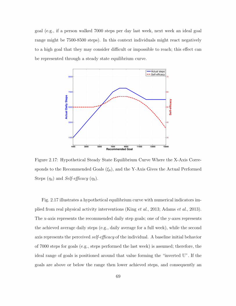
goal (e.g., if a person walked 7000 steps per day last week, next week an ideal goal

range might be 7500-8500 steps). In this context individuals might react negatively

to a high goal that they may consider difficult or impossible to reach; this effect can

be represented through a steady state equilibrium curve.

1000 3000 5000 7000 9000 11000 13000 15000

1000

3000

5000

7000

9000

Ac

tua

l D

aily

Ste

ps

1000 3000 5000 7000 9000 11000 13000 15000

30

40

50

60

70

Se

lf-e

ffic

ac

y

Recommended Goal

Actual stepsSelf-efficacy

Figure 2.17: Hypothetical Steady State Equilibrium Curve Where the X-Axis Corre-

sponds to the Recommended Goals (ξ8), and the Y-Axis Gives the Actual Performed

Steps (η4) and Self-efficacy (η3).

Fig. 2.17 illustrates a hypothetical equilibrium curve with numerical indicators im-

plied from real physical activity interventions (King et al., 2013; Adams et al., 2013).

The x-axis represents the recommended daily step goals; one of the y-axes represents

the achieved average daily steps (e.g., daily average for a full week), while the second

axis represents the perceived self-efficacy of the individual. A baseline initial behavior

of 7000 steps for goals (e.g., steps performed the last week) is assumed; therefore, the

ideal range of goals is positioned around that value forming the “inverted U”. If the

goals are above or below the range then lower achieved steps, and consequently an

69

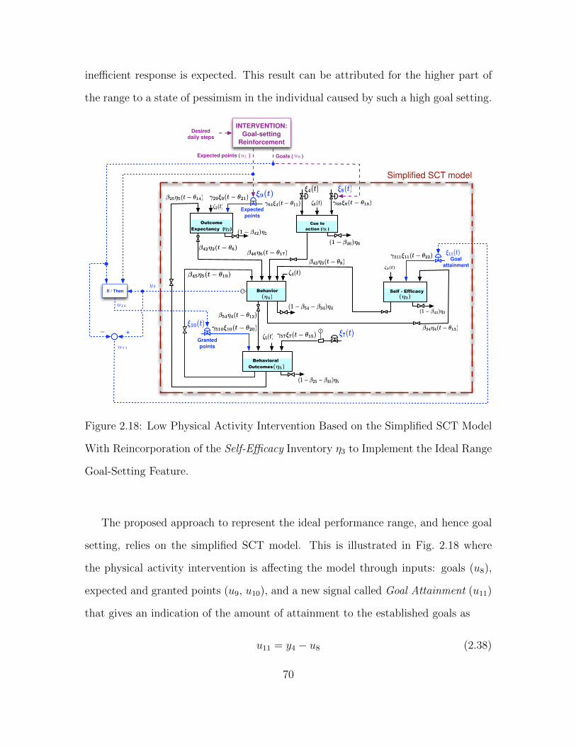
inefficient response is expected. This result can be attributed for the higher part of

the range to a state of pessimism in the individual caused by such a high goal setting.

Outcome

Expectancy ( )

Behavior

Behavioral

Outcomes

γ64ξ4(t − θ11)

Cue to

action ( )

γ57ξ7(t − θ15)

ξ4(t)

ξ7(t)

ζ2(t)

ζ4(t)

ζ5(t)

β42η2(t − θ6)

β54η4(t − θ12)

β25η5(t − θ14)

(1 − β54 − β34)η4

(1 − β42)η2

(1 − β25 − β45)η5

η2

(η4)

(η5)

ξ8(t)

γ68ξ8(t − θ18)ζ6(t)

(1 − β46)η6

β46η6(t − θ17)

η6

Fγ510ξ10(t − θ20)

β45η5(t − θ19)

γ29ξ9(t − θ21)

LT

Expected

points

Granted

points

INTERVENTION:

Goal-setting

Reinforcement

Goals ( )Expected points ( )

If / Then

Desired

daily steps

ξ9(t)

ξ10(t)

Self - Efficacy

ζ3(t)

β34η4(t − θ13)

β43η3(t − θ8)

(1 − β43)η3

(η3)

γ311ξ11(t − θ22)ξ11(t)

Goal

attainment

u11

u10

y4

u9 u8

Simplified SCT model

+_

Figure 2.18: Low Physical Activity Intervention Based on the Simplified SCT Model

With Reincorporation of the Self-Efficacy Inventory η3 to Implement the Ideal Range

Goal-Setting Feature.

The proposed approach to represent the ideal performance range, and hence goal

setting, relies on the simplified SCT model. This is illustrated in Fig. 2.18 where

the physical activity intervention is affecting the model through inputs: goals (u8),

expected and granted points (u9, u10), and a new signal called Goal Attainment (u11)

that gives an indication of the amount of attainment to the established goals as

u11 = y4 − u8 (2.38)

70

This signal is fed into the self-efficacy inventory such that if the individual fails to

reach a goal, a negative effect will be produced that ultimately will lead to a decrease

in performed behavior. The magnitude of this negative effect is quantified through

gains γ311 and parameter β43 .

To show the capability of the proposed approach to achieve an “inverted U”

and define the ideal range, a simulation was performed using the model depicted

in Fig. 2.18 with goals (u8) as the unique input, and considering θi = 0, ζj = 0

∀i, j. Performing the stability analysis described in Section 2.4.3 and considering the

effect from behavior (η4) to self-efficacy (η3), one of the sufficient stability conditions

detailed in (2.30) is

β34 < 1 (2.39)

Considering that the added signal u11 = y4 − u8 includes a linear dependency on the

inventory behavior (y4 = η4), the total effect from η4 to η3 is now β34 + γ311; hence

the previously discussed stability condition is modified as

β34 + γ311 < 1 (2.40)

Using the hypothetical representation from Fig. 2.17 and the semi-physical identi-

fication procedure described in Section 2.6, the following set of SCT model parameters

is selected to represent the ideal range of step-goals feature, and to satisfy the stability

sufficient conditions:

• τ2 = 28.26, τ3 = 876.07, τ4 = 20.19, τ5 = 25.98, τ6 = 0.06.

• γ29 = 1, γ64 = 1, γ68 = 1.01, γ33 = 1, γ510 = 1, γ57 = 1, γ35 = 1, γ36 = 1,

γ311 = 0.2.

• β25 = 0.12, β34 = 0.07, β42 = 0.27, β45 = 0.19, β46 = 0.13, β43 = 0.06, β54 = 0.01.

71

20 40 60 80 100 1200

5000

10000

15000

Time (days)

Ste

ps

Daily goals (u8=ξ

8)

Performed steps (y4=η

4)

20 40 60 80 100 120

-10000

-5000

0

Goal Attainment (ξ11

=u11

)

Ste

ps

20 40 60 80 100 12030

35

40

45

50

55

Self-efficacy (η3)

Level 0-1

00

Figure 2.19: Simulation Results for a Physical Activity Behavioral Intervention, Rep-

resenting the Ideal Range of Step-Goals Feature by Influencing Self-Efficacy (η3)

Through the Goal Attainment (u11) Signal.

72

Simulation results are shown in Fig. 2.19. During a few initial cycles, the per-

formed steps approximate the set goal. However, the magnitude of the difference

between the goal and the steps increases as observed in the goal attainment (u11)

signal, causing a considerable reduction in self-efficacy (η3) that eventually leads to a

considerable reduction of performed steps (y4 = η4). This approach must be carefully

verified via data obtained from system identification experiments, where it is cru-

cial to obtain well validated measurements for self-efficacy and the other SCT model

constructs.

2.8 Chapter Summary

This chapter describes how Social Cognitive Theory (SCT) can be represented as

a control systems model. Fluid analogy concepts were used to represent the dynamic

behavior portrayed in the theory; the analogy then was mathematically defined and

improved with the addition of a nonlinear section; after that, computational mod-

els were created to support visualization and validation efforts. Further, based on

the original narrative nature of the theory and the lack of specificity on some of the

interrelationships between constructs, especially over time, many challenges to the

creation of an effective control system model arose for determining the best represen-

tation of SCT from a control systems perspective. A path diagram from Structured

Equation Modeling (SEM) was also shown to present the ideas more clearly.

The simulations proved to be valuable for better specifying implicit assumptions

made within SCT to ensure better operationalization, for example the scenarios de-

picted the power of cue to action to strongly and rapidly influence behavior, much

more so than the cognitive constructs of SCT (e.g., self-efficacy, outcome expectan-

cies).

The comparison against the MILES data showed the ability of the model to depict

73

a real behavioral situation like physical activity. With an appropriate adaptation

process, the model could be extended beyond behavioral health scenarios.

Further studies are being developed to test the use and application of this model.

The structure of the model must be more thoroughly validated from experimental

data using semiphysical modeling principles. System identification techniques can be

used to better compare and contrast models; they should include an input design

stage that excites the most relevant components of the model.

The simulated scenarios proved the capability of the model to depict the habitu-

ation phenomena as it is described in the theory. There are some additional details

and approaches involved on the theory, such as overflow of reward structures (behav-

ioral outcomes), that could be described with the same strategy used for habituation;

furthermore both process could be modeled with more elaborate nonlinear schemes

that can improve the accuracy of the model.

A well identified feature for physical activity interventions, called the ideal range of

step goals, was incorporated into the model via a measurement of the goal achievement

that is directly fed into the self-efficacy inventory. Simulations helped to prove the

capability of this approach to represent the characteristic “inverted U” response when

this condition is activated.

74

Chapter 3

IDENTIFICATION TEST MONITORING PROCEDURE FOR

MULTIVARIABLE SYSTEMS

3.1 Overview

The accuracy of models obtained through system identification depends on the

quality of the gathered experimental data and the selected identification method.

The effect of external measurement conditions (e.g., noise) on model estimates can

be mitigated by judicious input signal design. One of the major challenges in system

identification is to obtain experiments that are sufficiently long and/or possess suf-

ficiently high signal to noise ratios such that system identification on the data leads

to useful models. Theoretical arguments favor experiments that are infinitely long

or have very high input magnitudes; however these conditions are in sharp contrast

to practical and economic constraints in real-life applications that demand shorter

experiments, constrained input signal magnitudes, and minimal manipulation of the

process actuators (Rivera et al., 2003). In particular, problems in process control and

adaptive interventions in behavioral health (Rivera, 2012) are application settings

where recognizing “plant-friendly” or “patient-friendly” concepts motivate system-

atic approaches to determining the necessary duration of identification experiments

(e.g., which can last months in the case of a behavioral health intervention).

To determine if the experimental data set is sufficiently informative, it is neces-

sary to define reliable indicators of the accuracy of the estimation process, such as

statistical uncertainties associated with the estimated parameters. Identification test

monitoring is a problem postulated by Rivera et al. (2003) that proposes an iterative

75

evaluation and refinement of input signals and experimental execution based on non-

parametric methods and uncertainty estimation. To obtain unbiased uncertainty de-

scriptions, periodic deterministic input signals are utilized, with the timespan defined

by one signal period defining an examination window for analysis of the identification

results. For system identification purposes, the Empirical Transfer Function Estima-

tion (ETFE) (Ljung, 1999) is used; it is an unbiased estimator for LTI systems subject

to periodic input signals. To compute statistical uncertainty regions for the ETFE

diverse methods have been proposed ((Bayard, 1993; Bayard and Hadaegh, 1994;

De Vries and Van den Hof, 1995)); these differ in the level of dependence on a priori

information available regarding the output noise structure, input design parameters,

and process dynamics.

In the first part of this chapter, a basic identification test monitoring procedure

is proposed from which the shortest possible experimental dataset resulting in an

acceptable model can be identified. The process is applied to a multivariable sys-

tem where the input signal is designed using a multisinusoidal “zippered” spectrum

(Rivera et al., 2009) to obtain independent-in-frequency inputs that enable the iden-

tification of individual transfer functions for each input-output combination. Each

period of the input signal is considered as the time window from which a statistical

uncertainty (using all data from initial to current time) is computed. Stopping cri-

teria for the experiment are defined based on the input-output element(s) of interest

and user-defined bounds. The final experimental duration will depend on pre-defined

design conditions (e.g., signal period, number of frequencies) and on external and

internal factors (e.g., measurement resolution, noise and system dynamics); hence

desirable (but not necessarily unique) results are obtained.

In the basic formulation, the outputs are measured after some time to account

for the transient effect. An estimate of the system’s transient response effect is not

76

considered because the number of cycles in a multisine signal is the only input de-

sign parameter that can be adjusted. Moreover the criterion utilized to stop the

experimental execution is solely based on percentage reduction in uncertainty during

consecutive iterations. To address these considerations the second part of the chap-

ter presents an enhanced identification test monitoring approach for MIMO systems

considering additional types of modifications in the input signal during experimental

execution. The additional modifications on the input signal are changes on the signal

amplitude and frequency content of the signals. To account for transient responses as

a result of changes in amplitude, the Local Polynomial Method (LPM) for periodic

signals (Pintelon et al., 2011) is utilized for computing transfer functions and uncer-

tainties. Two variations of the LPM are tested and contrasted: first to reduce the bias

in the estimation, the transient LPM (Monteyne et al., 2012) is applied over a set of

orthogonal-in frequency excited inputs constructed through the “zippered” spectral

design, secondly the fast LPM method (Pintelon et al., 2011) is applied over a set

of input signals with a full spectral design allowing a better frequency resolution but

increasing the bias on the estimate. The decision to make one or more of the spec-

ified modifications relies on operational constraints and user preferences. When the

input’s frequency content is re-defined, the new frequency grid makes use of harmonic

related values to retain a connection with previous estimates. To obtain a complete

estimate considering all the modifications performed during the experiment, an ag-

gregate estimator of the transfer functions and uncertainties is developed. Finally, a

stopping criterion for the experiment is presented that uses robust stability and ro-

bust performance metrics applied to the estimated uncertainty regions to guarantee

performance of a closed-loop system achievable from the identification data.

The chapter is organized as follows. Section 3.2 presents a basic identification test

monitoring procedure including the input signal design, an uncertainty estimation

77

procedure, and the proposed stopping criterion. Section 3.3 presents an enhanced

identification test monitoring procedure incorporating the possibility of modifications

in magnitude and harmonic frequency definition of the input signals. Additionally, an

enhanced stopping criterion based on robust control concepts is proposed. Section 3.4

is a simulation study that explores the proposed approaches on a heavy oil fractionator

plant model. Section 3.5 gives summary and conclusions of the chapter.

3.2 Basic Identification Test Monitoring Procedure Based on Statistical

Uncertainty Estimates

3.2.1 Background and Input Signal Design

Consider a sampled-data multiple-input multiple-output (MIMO) system with

nu ∈ N inputs and ny ∈ N outputs that can be described by

y(k) = G(q)u(k) + v(k) (3.1)

where u ∈ Rnu and y ∈ Rny are the input and output vectors respectively, v ∈ Rny

is the output disturbance vector and G(q) is the ny × nu transfer function matrix

representing the multivariable LTI plant. Each SISO transfer function G[m,n](q) rep-

resents the relationship between an input un and an output ym for m = 1 . . . ny, and

n = 1 . . . nu.

Using an output noise model as is illustrated in Fig. 3.1, any output ym can be

represented by the effect of all the nu inputs and the respective output noise vm as

ym(k) = G[m,1](q)u1(k) + · · ·+G[m,nu](q)unu(k) + vm(k), m = 1, . . . , ny (3.2)

Many identification approaches can be used to obtain the transfer function ma-

trix G(q), however frequency domain methods (Bayard, 1993; Bayard and Hadaegh,

1994) offer convenient properties that may result in an appropriate uncertainty es-

78

G[1,1](q)

G[Ly,1](q)

G[1,Lu](q)

G[Ly,Lu](q)+

+

+

+

++

u1

uLu

y1

yLy

+

+

+

+

vLy

v1

to G[2,1](q)

to G[Ly−1,Lu](q)

from G[1,2](q)

from G[Ly,Lu−1](q)

+

+

Figure 3.1: Block Diagram for the MIMO System Describing the Effect of an Indi-

vidual SISO Transfer Function G[m,n] Over the Outputs.

timation. Instead of running nu independent Single-Input Multiple-Output (SIMO)

experiments with nu different excitation signals, the proposed approach will consist

in one experiment where the inputs are acting simultaneously, but each one is excited

over an orthogonal grid of frequencies such that each G[m,n] can be independently

estimated.

For system identification, the averaged Empirical Transfer Function Estimation

(ETFE) method will be used. If the input signals are designed to be periodic (e.g.,

multisinusoidal signals), uncertainty bounds can be calculated using statistical ap-

proaches (Bayard, 1993; De Vries and Van den Hof, 1995; Pintelon and Schoukens,

2012). The general conditions for the existence of the averaged ETFE and the pro-

posed uncertainty bounds are

• The true plant G(q) is exponentially stable, linear and time invariant.

79

• Each output disturbance noise vm(k), m = 1, . . . , ny can be written as vm(k) =

Hm(q)am(k) where am(k) is a normalized white Gaussian zero-mean noise se-

quence, and Hm(q) is a linear filter that can be decomposed as Hm(q) =

σmHm(q) where σm <∞ is scalar and Hm(q) is an stable transfer function.

Multisine inputs are deterministic and periodic signals whose spectrum can be

directly specified by the designer. One period of the input un can be described by

un(k) = λn

Ns/2∑j=1

√2α[n,j] cos(ωjkTs + φ[n,j])

ωj = 2πjNsTs

, k = 1, . . . , Ns

(3.3)

where λn is the scaling factor, Ns is the signal period, Ts is the sampling time. For

each harmonic: α[n,j] is a factor used to specify the relative power of the harmonic, ωj

is the frequency, and φ[n,j] is the phase. The input signal will be repeated M cycles

such that the total length of the signal is

N = NsM (3.4)

The coefficients α[n,j] must be chosen to obtain input signals that are excited

orthogonally in frequency. Two signals are orthogonal if a nonzero Fourier coefficient

in a specific frequency of one signal implies a zero-valued Fourier coefficient at the

same frequency for the other signal; this is called a “zippered” spectra design and was

introduced by Rivera et al. (2009). If ns is defined as the total number of independent

excited sinusoids considering the nu inputs, the total number of harmonics nh can be

defined as

nh = ns (3.5)

The spectrum for each signal un, n = 1, . . . nu can be constructed by specifying each

80

2πNsTs

2πns

NsTs

πTs

Frequency

Fo

urie

r co

effi

cie

nts

(ω)

= u1= u2

Figure 3.2: Conceptual Representation for a nu = 2 Channel “Zippered” Spectra

Design With ns = 6 Independently Excited Sinusoids, Giving nh = 6 Harmonics and

Selecting Ns = 18.

α[n,j] as

α[n,j] =

1 if j = nu(i− 1) + n for i = 1, 2, . . . ns

0 otherwise

(3.6)

A conceptual representation of the zippered design for nu = 2 inputs is presented in

Fig. 3.2.

The signal period Ns must be carefully selected to meet the problem requirements;

it should be long enough to capture the dynamics of the system, but at the same as

short as possible since it will represent the resolution (time decision window) of the

monitoring process. A starting point can be to select the required number of sinusoids

per channel ns; if some information is available about the model order and since ns

81

represents the number of persistent excitation then

Model order ≤ ns (3.7)

The range of usable frequencies is given by (3.3) as

2π

NsTs≤ ω ≤ 2πns

NsTs<

π

Ts(3.8)

from where a bound for Ns can be derived as

Ns > 2ns (3.9)

therefore the total duration of the experiment N (in terms of sampling instants) is

N = NsM > 2nsM (3.10)

If no further information about the system is available, the minimum period Ns =

2ns + 1 can be selected. If some information is available about the dominant time

constants of the system τLdom and τHdom, frequency bounds ω∗ and ω∗ can be defined as

1

βsτHdom= ω∗ ≤ ω ≤ ω∗ =

αsτLdom

(3.11)

where αs and βs are parameters that respectively specify high and low ranges of

interest in the signal. Using a similar procedure to the one developed by Rivera et al.

(2009), the following bounds can be defined to confirm or modify the values of ns and

Ns

2π

NsTs≤ ω∗ ≤ ω ≤ ω∗ ≤ 2πns

NsTs<

π

Ts(3.12)

from where

Ns ≥2π

ω∗Tsand Ns ≤

2πnsω∗Ts

(3.13)

82

combining the two sides from (3.12) a bound for the bandwidth can be defined as

ω∗ − ω∗ ≤2π

NsTs(ns − 1) (3.14)

If Ns is replaced with the lower bound from (3.13) then

ω∗ − ω∗ ≤ ω∗(ns − 1) (3.15)

ω∗

ω∗− 1 ≤ ns − 1 (3.16)

Consolidating results from (3.16), (3.13), and (3.9) the final bounds can be ex-

pressed as

ns ≥ω∗

ω∗(3.17)

max

(2ns,

2π

ω∗Ts

)≤ Ns ≤

2πnsω∗Ts

(3.18)

One option for phase selection is to use the approach of Schroeder (1970), designed

to minimize peaking in the time domain as:

φ[n,j] = 2π

j∑ci=1

ci.α[n,ci] (3.19)

If low variability on the input signals is of special importance, a modification can be

used based on the crest factor (CF) index; CF is defined by the ratio of the Chebyshev

(infinity) norm versus the 2-norm:

CF (un) =`∞(un)

`2(un)(3.20)

The crest factor provides a measure of the distribution of the signal values over the

input span. A low crest factor indicates that most of the values are located near the

maximum and minimum of the sequence, thus avoiding infrequent and comparatively

high peak values.

Harmonic phases will be selected to minimize the crest factor of the signal using

the approach proposed by Guillaume et al. (1991), where an approximation of the

83

minimization of the Chebyshev norm is proposed by sequentially minimizing the `p

norm for p = 4, 8, 16, . . . based on Polya’s algorithm which states that:

limp→∞

pp = p∞ (3.21)

where p = [φ[n,1] φ[n,2] . . . φ[n,ns]]> is the phase vector for (3.3) and p∞ is the

minimax solution considering that the 2-norm remains invariant with respect to the

phases φ[n,j]. This is in general a nonlinear optimization problem and performs better

than other crest factor minimization techniques (Guillaume et al., 1991).

3.2.2 Uncertainty Description

3.2.2.1 Transfer Function Estimation

Since each un is designed orthogonally in frequency, it is possible to find inde-

pendent estimates for every transfer function element. Assume that M periods of

input/output data un(k), ym(k) are collected and denote the output data from the

lth period as

ylm(k) = ym(k + (l − 1)Ns)

k = 1 . . . Ns, l = 1 . . .M

(3.22)

The Discrete Fourier Transforms (DFT) for each input and output are defined by

Un(ωj) =1√Ns

Ns∑k=1

un(k)e−iωjkTs ; n = 1, . . . , nu (3.23)

Y lm(ωj) =

1√Ns

Ns∑k=1

ylm(k)e−iωjkTs ; m = 1, . . . , ny (3.24)

for ωj = 2πjNsTs

, j = 1, 2 . . . nsnu (3.25)

For periodic inputs the ETFE is an unbiased estimation and is defined only for a

fixed number of frequencies (Ljung, 1999). The averaged ETFE is computed as

G[m,n](ωni ) =

Ym(ωni )

Un(ωni )(3.26)

84

with Ym(ωni ) =1

M

M∑l=1

Y lm(ωni ) (3.27)

where ωni ∈ W n, and W n is the frequency grid defined by the zippered design for

input n as a subset of the complete grid shown in (3.25), specified by

W n = {ωni ∈ R | ωni = 2π[nu(i−1)+n]NsTs

, i = 1, 2, . . . , nsch} (3.28)

and nsch is the total number of harmonics excited per input channel defined as

nsch =nsnu

(3.29)

3.2.2.2 Survey of Statistical Uncertainty Computation Methods

Diverse approaches have been developed for the computation of statistical un-

certainties from the ETFE over periodic inputs; the main differences between these

are:

• Existence of a priori knowledge of the design parameters of the periodic input

signal, such that the Fourier coefficients of the spectrum can be derived.

• Existence of a priori knowledge of the noise coloring filter Hm(q).

• Requirement that data be collected at periodic steady-state

A first approach presented by Bayard (1993), relies on a simultaneous estimation

of the transfer function as a regression problem using a Gauss-Markov formulation,

where it is necessary to use the α[n,j] factors from the input spectral definition pre-

sented in (3.3). It is assumed that the data is taken at periodic steady-state. The

noise coloring filter Hm(q) is known, and σm may be either known or unknown. If σm

is unknown it can be estimated using the regression approach as

σ2m =

M∑l=1

ns∑i=1

∣∣Ym(ωni )− Y lm(ωni )

∣∣2Ns(NsM − 2nsch)

, ωni ∈W n (3.30)

85

ℓ1−ρa[m,n]

Re{G[m,n](ωni )}

Im{G[m,n](ωni )}

Figure 3.3: Conceptual Representation of the 100 × (1 − ρ)% Confidence Region

for G[m,n](ωni ) Over a Nyquist Frequency Response Plot for a Specific Frequency

ωni ∈W n.

The confidence region is conceptually illustrated in Fig. 3.3, where it can be seen

in a Nyquist plot as a circle centered in G[m,n](ωni ) of radius `1−ρ

a[m,n] equal to

[`1−ρa[m,n](ω

ni )]2

=2σ2

m|Hm(ωni )|2α[n,j]NsM

F1−ρ(2, NsM − 2nsch) (3.31)

where α[n,j] is given by (3.6), and F1−ρ(ν1, ν2) is the 100 × (1 − ρ)% percentile of a

Fisher distribution with ν1 and ν2 degrees of freedom such that

Prob{∣∣G[m,n](ω

ni )−G[m,n](ω

ni )∣∣ ≤ `1−ρ

a[m,n](ωni )}

= 1− ρ (3.32)

An extension for the MIMO case was presented by Bayard and Hadaegh (1994),

where an expression of the filter Hm(q) is no longer required. From a practical stand-

point this improvement is very important since precise knowledge of the noise struc-

ture may be difficult to obtain. However the price to be paid is that results are valid

only asymptotically. In this case an estimation of the output noise variance for each

86

frequency is given as

|Hm(ωni )|2 =

M∑l=1


∣∣2Ns(M − 1)

(3.33)

The resultant additive uncertainty norm-bound for a 100×(1−ρ)% confidence region

is

[`1−ρa[m,n](ω

ni )]2

=2|Hm(ωni )|2α[n,j]NsM

F1−ρ(2, 2M − 2) (3.34)

One minor drawback of this method is that still requires the use of the Fourier coef-

ficients α[n,j] from the multisine definition.

In this work, an uncertainty description that does not require specific knowledge

of the noise filter Hm(q) and the input spectral definition will be used. However,

it still requires periodic steady-state data. One uncertainty computation method

that includes effects of unmodeled dynamics and transient responses can be found in

(De Vries and Van den Hof, 1995). It incorporates hard error bounds to deal with

the transient response problems while making the estimation more conservative.

3.2.2.3 Additive Uncertainty Calculation

The proposed approach does not require a priori information about the input

spectra and the noise filter structure, but the data needs to be measured at periodic

steady-state. The noise variance is computed from transfer function estimation rather

than from the output measurement only. The following expressions are referred to

the frequency grid for ωni defined in (3.28). Under the specified conditions it can be

shown (Bayard, 1993; Pintelon and Schoukens, 2012) that

|G[m,n](ωni )−G[m,n](ω

ni )|2

σ2G[m,n]

(ωni )∼ F (2, 2M − 2) (3.35)

87

where F (ν1, ν2) denotes a Fisher distribution with ν1 and ν2 degrees of freedom, and

σ2G[m,n]

(ωni ) is the sample variance of the averaged ETFE.

Since the ETFE was obtained from an averaging procedure, and following standard

results from probability theory, its variance can be derived from the variance of the

real transfer function G[m,n] as

σ2G[m,n]

(ωni ) =σ2G[m,n]

(ωni )

M(3.36)

and using sample variances

σ2G[m,n]

(ωni ) =σ2G[m,n]

(ωni )

M(3.37)

the sample variance of G[m,n] can be estimated as

σ2G[m,n]

(ωni ) =1

M − 1

M∑l=1

|Ym(ωni )− Y lm(ωni )|2

|Un(ωni )|2 (3.38)

from here it follows that

σ2G[m,n]

(ωni ) =1

M(M − 1)

M∑l=1


|Un(ωni )|2 (3.39)

As was previously noted, the additional division by M is due to averaging in the

estimates (Pintelon and Schoukens, 2012).

For a duration of M periods, the 100 × (1 − ρ)% confidence region can be con-

structed as a circle with center G[m,n](ωni ) and radius `1−ρ

a[m,n](ωni ,M) where

[`1−ρa[m,n](ω

ni ,M)

]2= σ2

G[m,n](ωni )F1−ρ(2, 2M − 2) (3.40)

An explicit dependence on the period M in the uncertainty definition has been added

for use in the definition of the monitoring process. Estimated uncertainty bounds are

asymptotic; small values of M result in conservative estimates.

88

A multivariable uncertainty computation approach that involves all the transfer

function elements can also be specified (Bayard and Hadaegh, 1994); this will con-

stitute a more general but conservative estimate. Model uncertainty constituting the

maximum singular value at each frequency grid point with probability 1 − κ can be

characterized by

Prob{σ(G(ωni )−G(ωni )

)≤ ε1−κ(ωni )

}= 1− κ (3.41)

The well known Frobenious norm bound can be considered over the square of the

maximum singular value as

σ(G(ωni )−G(ωni )

)2 ≤ ‖G(ωni )−G(ωni )‖2f (3.42)

=nu∑n=1

ny∑m=1


ni )|2 (3.43)

Each of the terms in (3.43) can be overbounded to probability 1− ρ by

∣∣G[m,n](ωni )−G[m,n](ω

ni )∣∣2 ≤ [`1−ρ

a[m,n](ωni ,M)

]2(3.44)

with `1−ρa[m,n](ω

ni ,M) calculated in (3.40). The events in (3.43) are statistically inde-

pendent since each output is generated from a different Gaussian source and each

input is defined orthogonally in frequency; hence the event


)2 ≤nu∑n=1

ny∑m=1

[`1−ρa[m,n](ω

ni ,M)

]2,[ε1−κ(ωni ,M)

]2(3.45)

holds with probability

1− κ = (1− ρ)ny ·nu (3.46)

3.2.2.4 Extension to a Parallel Connected System

Consider that the system to be identified contains two transfer functions G[m,n] and

S[m,n] that operate in parallel over the output as shown in Fig. 3.4; assume also that

89

un ym

vm

G[m,n]

S[m,n](q)

G[m,n](q)+ +

+ +

Figure 3.4: Block Diagram of a Modified System Including the Effect of a Transfer

Function S[m,n](q) Connected in Parallel With G[m,n](q).

individual estimations for each transfer function are required. Regular identification

procedures are not able to process the information to obtain independent estimates of

G[m,n] and S[m,n]. Semi-physical identification methods (e.g., grey box) (Lindskog and

Ljung, 1995) can solve the problem by using a-priori known partial information of the

models, together with the experimental inputs and outputs. Under these conditions

it is interesting to check the validity of the calculated uncertainties as indicators of

the output noise effect over the estimation.

Considering the original system without the addition of S[m,n] and using (3.1)

ym(k) = G[m,n](q)un(k) + vm(k) (3.47)

Y lm(ωni ) = G[m,n](ω

ni )Un(ωni ) + V l

m(ωni ),

l = 1, . . . ,M

(3.48)

where V lm(ωni ) is the DFT for the lth period of the output noise signal vm(k). The

averaged DFT of the output is

Ym(ωni ) =1

M

M∑l=1

[G[m,n](ω

ni )Un(ωni ) + V l

m(ωni )]

(3.49)

Ym(ωni ) = G[m,n](ωni )Un(ωni ) + Vm(ωni ) (3.50)

90

where Vm(ωni ) =1

M

M∑l=1

V lm(ωni ) (3.51)

From (3.39)

σ2G[m,n]

(ωni ) =1

M(M − 1)

Hm(ωni )

|Un(ωni )|2 (3.52)

with Hm(ωni ) =M∑l=1

|Ym(ωni )− Y lm(ωni )|2 (3.53)

substituting (3.48) and (3.50) in (3.53)

Hm(ωni ) =M∑l=1

∣∣G[m,n](ωni )Un(ωni ) + Vm(ωni )−G[m,n](ω

ni )Un(ωni )− V l

m(ωni )∣∣2 (3.54)

Hm(ωni ) =M∑l=1

∣∣Vm(ωni )− V lm(ωni )

∣∣2 (3.55)

By replacing Hm(ωni ) in (3.52) and (3.40) it can be seen that the computed additive

uncertainty `1−ρa[m,n](ω

ni ,M) depends only on the effect of the output noise vm(k), and

not on G[m,n].

If the system depicted in Fig. 3.4 is now considered including S[m,n](q) the output

is

ym(k) = G[m,n](q)un(k) + S[m,n](q)un(k) + vm(k) (3.56)

Previous derivations are recomputed as

Y lm(ωni ) = G[m,n](ω

ni )Un(ωni ) + S[m,n](ω

ni )Un(ωni ) + V l

m(ωni ) (3.57)

˜Ym(ωni ) = G[m,n](ωni )Un(ωni ) + S[m,n](ω

ni )Un(ωni ) + Vm(ωni ) (3.58)

The variance of the ETFE is now

σ2˜G[m,n]

(ωni ) =1

M(M − 1)

Hm(ωni )

|Un(ωni )|2 (3.59)

with Hm(ωni ) =M∑l=1

| ˜Ym(ωni )− Y lm(ωni )|2 (3.60)

91

and

Hm(ωni ) =M∑l=1

∣∣∣[G[m,n](ωni ) + S[m,n](ω

ni )]Un(ωni ) + Vm(ωni )

−[G[m,n](ω

ni ) + S[m,n](ω

ni )]Un(ωni )− V l

m(ωni )∣∣∣2

(3.61)

Hm(ωni ) =M∑l=1

∣∣Vm(ωni )− V lm(ωni )

∣∣2 (3.62)

therefore

Hm(ωni ) = Hm(ωni ) (3.63)

This result shows once again that the computed uncertainty depends only on the

portion due to the output noise on ym. It can serve as a measurement of the output

noise effect on the capability of the experimental data set to identify the system

adequately.

3.2.2.5 Error-In-Variables Uncertainty Description

In this section the error-in-variables case (Soderstrom et al., 2007) is considered;

this scenario is depicted in Fig. 3.5 for an specific input-output element G[m,n], where

both inputs and outputs are corrupted by external noise as

un(k) = u0n(k) + xn(k) (3.64)

ym(k) = y0m(k) + vm(k) (3.65)

u0n and un are the designed input and the measured input respectively, while xn is the

input measurement noise. The measured output ym is defined as shown in (3.2) with

y0m(k) = G[m,1](q)u

01(k) + · · ·+G[m,nu](q)u

0nu(k) (3.66)

Such circumstances may exist when the input signal is not fully designed by the user,

but has an underlying periodic character and can be measured. Uncertainty bounds

92

G[m,n](q)+

+ +

+

un

ym+

vm

+

xn

u0n

y0m

++

Figure 3.5: Block Diagram Showing the Error-In-Variable Setting for Input n and

Output m of a MIMO System.

can still be computed; however, calculating the estimation variance must consider the

variability on the input measurement. The lth period of the nth measured input signal

is

uln(k) = un(k + (l − 1)Ns)

k = 1 . . . Ns, l = 1 . . .M

(3.67)

and its DTF is defined as

U ln(ωj) =

1√Ns

Ns∑k=1

uln(k)e−iωjkTs ; n = 1, . . . , nu

for ωj = 2πjNsTs

, j = 1, 2 . . . nsnu

(3.68)

for ωni ∈W n the mean value of Un is

Un(ωni ) =1

M

M∑l−1

U ln(ωni ) (3.69)

and the ETFE is now

G[m,n](ωni ) =

Ym(ωni )

Un(ωni )(3.70)

The sample variances and covariance of Un and Ym are

σ2Un(ωni ) =

1

M − 1

M∑l=1

∣∣Un(ωni )− U ln(ωni )

∣∣2 (3.71)

93

σ2Ym(ωni ) =

1

M − 1

M∑l=1


∣∣2 (3.72)

σ2YmUn(ωni ) =

1

M − 1

M∑l=1

[(Ym(ωni )− Y l

m(ωni ))·(Un(ωni )− U l

n(ωni ))]

(3.73)

It can be shown (Pintelon and Schoukens, 2012) that the sample variance of the

ETFE for this case can be computed as

σ2G[m,n]

(ωni ) =|G[m,n](ω

ni )|2

M

(σ2Ym

(ωni )

|Ym(ωni )|2 +σ2Un

(ωni )

|Un(ωni )|2 − 2 Re

{σ2YmUn

(ωni )

Ym(ωni )Un(ωni )

})(3.74)

and the additive uncertainty `1−ρa[m,n](ω

ni ,M) can be computed using (3.40) again.

Note that if no noise exists in the input (i.e., the input is measured as designed),

then Un(ωni ) = U ln(ωni )(l = 1, . . . ,M) = Un(ωni ); therefore σ2

Un(ωni ) = 0, σ2

YmUn(ωni ) =

0, and equation (3.74) is transformed into (3.39).

3.2.3 Derivation of a Monitoring Procedure

As noted in the Overview section, the goal is to find the shortest experiment

that is sufficiently informative based on a specified uncertainty level. The monitoring

procedure is performed by incrementing the number of periods M one at a time

(starting from M = 2 because of averaged ETFE), such that with each increment on

M the total duration of the experiment will be NsT time units longer.

Using a worst-case criterion, a maximum additive uncertainty is computed over

the frequency grid for ωni defined in (3.28) for each input/output element as

˜a[m,n](M) = max

ωni ∈Wn

[`1−ρa[m,n](ω

ni ,M)

], M = 2, 3 . . . (3.75)

Uncertainty values by themselves are not meaningful for the monitoring process,

instead percentages of reduction in ˜a[m,n](M) among successive values of M are cal-

94

culated

AV [m,n](M) =ã[m,n](M − 1)− ˜

a[m,n](M)

ã[m,n](2)

× 100 (3.76)

RV [m,n](M) =ã[m,n](M − 1)− ˜

a[m,n](M)

ã[m,n](M − 1)

× 100 (3.77)

M = 3, 4 . . .

where AV[m,n] is the absolute percentage reduction referred to the first estimate (M =

2), and RV[m,n] is the relative percentage reduction referred to the previous value of

M .

Depending on the system, the set of all the (m,n) elements of interest can be

defined as

O ={

(m ∈ N, n ∈ N) | 1 ≤ m ≤ ny, 1 ≤ n ≤ nu,

effect from input n to output m is of interest} (3.78)

This definition allows the use of one or more of the transfer function elements.

Using the worst case scenario criterion, maximum percentages of uncertainty re-

duction within all input-output directions are defined as

AV (M) = max(m,n)∈O

AV [m,n](M), M = 3, 4 . . . (3.79)

RV (M) = max(m,n)∈O

RV [m,n](M), M = 3, 4 . . . (3.80)

The stopping criterion will determine when the percentage changes on uncertain-

ties have reached a predefined minimum bound for a determined amount of continuous

iterations, and therefore the experiment can be stopped. If BAV and BRV are defined

as the maximum allowed percentages of reduction in the last nMi consecutive unitary

increments of M , then the stopping criterion can be

Stop at M = Q− 1 when

AV (Q− r) ≤ BAV and RV (Q− r) ≤ BRV

for r = 1, . . . , nMi consecutive iterations

(3.81)

95

Lower values of BAV and BRV , or a higher nMi, will result in more accurate but longer

experiments.

Maximum additive uncertainty for the general multivariable case can also be com-

puted using the bound ε1−κ(ωni ,M), defined in (3.45)

ε(M) = maxωni ∈W

n

[ε1−κ(ωni ,M)

], M = 2, 3 . . . (3.82)

and percentages of uncertainty reduction can be redefined for M = 3, 4 . . . as

AV (M) =ε(M − 1)− ε(M)

ε(2)× 100 (3.83)

RV (M) =ε(M − 1)− ε(M)

ε(M − 1)× 100 (3.84)

Based on the definitions in (3.83) and (3.84), the stopping criteria presented in (3.81)

can be used.

3.3 Enhanced Identification Test Monitoring Procedure Relying on Uncertainty

Estimates

3.3.1 Background

Consider the sampled-data multiple-input multiple-output (MIMO) system pre-

sented in Section 3.2.1 with nu ∈ N inputs and ny ∈ N outputs, and described by

y(k) = G(q)u(k) + v(k) (3.85)

where u ∈ Rnu and y ∈ Rny are the input and output vectors respectively, v ∈ Rny

is the output disturbance vector and G(q) is the ny × nu transfer function matrix

representing the multivariable LTI plant. Each SISO transfer function G[m,n](q) rep-

resents the relationship between an input un and an output ym for m = 1 . . . ny, and

n = 1 . . . nu.

96

To perform the proposed identification test monitoring procedure, uncertainties

are obtained through the computation of frequency domain transfer function esti-

mates. The conditions assumed for the validity of the proposed uncertainty compu-

tation method are repeated here for clarity:

• The true plant G(q) is exponentially stable, linear and time-invariant.

• The output disturbance noise vm(k), m = 1, . . . , ny can be written as vm(k) =

Hm(q)am(k) where am(k) is a normalized white Gaussian zero-mean noise se-

quence. Hm(q) is a linear filter that can be decomposed as Hm(q) = σmHm(q)

where σm <∞ is scalar and Hm(q) is a stable transfer function.

Random phase multisine input signals are used again as these allow direct speci-

fication of the frequency spectrum by the user, independent of the selected transfer

function computational method. The monitoring procedure considered in this section

allows changes on the input signals during experimental execution. These changes

can be in amplitude, and/or frequency content of the signals. The Empirical Transfer

Function Estimates (ETFE) method used in Section 3.2.2 did not account for tran-

sient effects due to the on-the-go input signal modifications, and hence this step has

to be re-examined.

3.3.1.1 The Local Polynomial Method

The Local Polynomial Method (LPM; Pintelon et al. (2010)) is used to compute

transfer functions in the frequency domain considering the system and noise transient

(leakage) errors as a function of the frequency. This is done by approximating locally

the frequency response function and the transient errors with a low degree polyno-

mial. If N samples of the system outputs, disturbed by filtered white noise v(k), are

measured with a sampling time Ts, then the basic assumption of the LPM for MIMO

97

systems is that the output spectra satisfy

Y (ωj) = G(ωj)U(ωj) + T (ωj) + V (ωj) (3.86)

where:

• Y (ωj) ∈ Rny is the discrete Fourier transform (DFT) of the noisy N samples of

the ny outputs.

• G(ωj) is the ny × nu true frequency response transfer function matrix of the

system.

• U(ωj) ∈ Rnu is the DFT of the true N samples of the nu inputs.

• T (ωj) ∈ Rny is the total system and noise transient term.

• V (ωj) ∈ Rny is the MIMO output noise.

• ωj = 2πjNTs

, j = 1, . . . , N .

Since the transient and the transfer function terms are assumed to be smooth func-

tions of the frequency, they can be locally approximated by low-order polynomials:

T (ωj+r) = T (ωj) +R∑s=1

ts(j)rs +OT (3.87)

G(ωj+r) = G(ωj) +R∑s=1

gs(j)rs +OG (3.88)

where OT = N−1/2O((r/N)R+1) and OG = O((r/N)R+1) are the remainders of the

Taylor series expansions around ωj of order R + 1 for T and G, as is explained with

more details in (Pintelon et al., 2010).

Two variants of the LPM are considered in the proposed monitoring process: LPM

for arbitrary excitations for transition cycles when only one period of the signals is

available, and LPM for periodic excitations when two or more periods of data are

available.

98

3.3.1.2 LPM for Arbitrary Excitations

This approach is used only immediately after a change (amplitude or frequency

content) on the input signal has occurred, and only one period of the signal is avail-

able. The vector of unknown parameters is

ΘA,j = [G(ωj) g1(j) · · · gR(j) T (ωj) t1(j) · · · tR(j)] (3.89)

where ΘA,j ∈ Cny×(R+1)(nu+1). To estimate G(ωj), the method considers nA neighbor-

ing frequencies around each side of wj, then by combining (3.86), (3.87) and (3.88)

the folowing expressions are derived:

Y A,j = ΘA,jKA,j + V A,j (3.90)

with Y A,j = [Y (ωj−nA) · · ·Y (ωj) · · ·Y (ωj+nA)] (3.91)

V A,j = [V (ωj−nA) · · ·V (ωj) · · ·V (ωj+nA)] (3.92)

KA,j =

p(−nA)⊗ U(ωj−nA)T p(−nA)

......

p(0)⊗ U(ωj)T p(0)

......

p(nA)⊗ U(ωj+nA)T p(nA)

T

(3.93)

V A,j = [V (ωj−nA) · · ·V (ωj) · · ·V (ωj+nA)] (3.94)

p(r) = [1 r1 · · · rR] (3.95)

where Y A,j,V A,j ∈ Cny×2nA+1, KA,j ∈ C(R+1)(nu+1)×2nA+1, and ⊗ is the operator for

the Kronecker product. Using a linear least squares (LLS) approximation an estimate

of ΘA,j at ωj is

ΘA,j = Y A,jKHA,j(KA,jK

HA,j)

−1 (3.96)

99

where XH denotes the Hermitian transpose of X. From here

G(ωj) = ΘA,j

Inu×nu

0R(nu+1)+1×nu

(3.97)

The number of frequency points used for the local estimation at each frequency

ωj is 2nA + 1, as can be observed in (3.91) – (3.94). This band becomes assymetrical

when ωj is close to the boundaries causing larger estimation errors (Pintelon et al.,

2010). For higher values of R, the matrix KA,j can become ill conditioned. Based on

the dimension of KA,j the number of degrees of freedom is defined as

dfA = 2nA + 1− (R + 1)(nu + 1) (3.98)

This term quantifies the number of independent noise residuals in

V A,j = Y A,j − ΘA,jKA,j (3.99)

from where an estimate of the noise covariance matrix can be found as

CV (ωj) =1

dfAV A,jV

H

A,j (3.100)

To compute uncertainty bounds a sufficient condition (Pintelon et al., 2010) is

dfA ≥ ny (3.101)

The parameters must be carefully selected to accomplish (3.101) using the minimum

possible nA and an acceptable value for R (R = 2 is often a good selection (Pintelon

et al., 2010)).

An estimate for the transfer function covariance matrix can be defined as

CG(ωj) = SHS ⊗ CV (ωj) (3.102)

where X represents the complex conjugate of X, and

S = KHA,j(KA,jK

HA,j)

−1

Inu×nu

0R(nu+1)+1×nu

(3.103)

100

3.3.1.3 LPM for Periodic Excitations

This approach is used during the monitoring process when M periods (M ≥ 2)

of the input signals are available. Because of the presence of more than one period,

the DFT of the output signals includes frequencies where the inputs are excited and

others non-excited. The main assumption is that the system and noise transient

errors are present at both excited and non-excited frequencies, while the steady state

system response is only present at the excited ones, as depicted in Fig. 3.6. Given the

assumed Gaussian nature of the noise and the smoothed-in-frequency nature of the

transient response, the method is divided in two parts: an estimation of the transient

response based on the non-excited lines, followed by the computation of the system

transfer function over the excited lines (Pintelon et al., 2011).

DFT

outputs

ω

Excited frequencies

ω1M ω2M ω3M

Figure 3.6: Excited and Non-Excited Frequency Components According to the Peri-

odic LPM, Where Solid Lines Correspond to the System Response and Dashed Lines

are the Transient and Noise Contributions.

Non-excited frequencies

Using the complete M periods for the DFT computation, the excited frequencies

correspond to ωjM for j = 1, · · · , N . The steady state system response is zero at

101

the non-excited frequencies ωjM+r for r = ±1, · · · ,±(M − 1), hence at those points

(3.86) can be reduced as

Y (ωjM+r) = T (ωjM+r) + V (ωjM+r) (3.104)

The transient term at those frequencies is approximated as

T (ωjM+r) = T (ωjM) +R∑s=1

ts(j)rs +OTne (3.105)

where OTne = (MN)−1/2O((r/(MN))R+1) is the remainder that is explained with

details in (Pintelon et al., 2011). The estimation is performed using 2nT non-excited

frequencies around the excited frequency ωjM , resulting in the following equations:

Y T,jM = ΘT,jMKT,jM + V T,jM (3.106)

with Y T,jM = [Y (ωjM−rnT ) · · ·Y (ωjM+rnT)] (3.107)

ΘT,jM = [T (ωjM) t1(jM) · · · tR(jM)] (3.108)

V T,jM = [V (ωjM−rnT ) · · ·V (ωjM+rnT)] (3.109)

KT,jM = [p(−rnT )T · · · p(rnT )T ] (3.110)

where Y T,jM ,V T,jM ∈ Cny×2nT , ΘT,jM ∈ Cny×R+1, KT,jM ∈ CR+1×2nT , and p(r)

as was defined in (3.95). Using the same LLS estimator the vector of unknowns is

approximated as

ΘT,jM = Y T,jMKHT,jM(KT,jMK

HT,jM)−1 (3.111)

from where the noise and system transient response is obtained as

T (ωjM) = ΘT,jM

1

0R×1

(3.112)

Based on the dimension of KT,jM the number of degrees of freedom is dfT = 2nT −

(R + 1). This term quantifies the number of independent noise residuals in

V T,jM = Y T,jM − ΘT,jMKT,jM (3.113)

102

from where an estimate of the noise covariance matrix can be found as

CVT (ωjM) =1

dfTV T,jM V

H

T,jM (3.114)

To ensure that the noise covariance estimate has the same rank as its real counterpart,

the condition

dfT ≥ ny + nu (3.115)

must be satisfied. With the derived estimates of the transient response at the excited

frequencies, a transient-free estimate of the output DFT at those frequencies can be

defined as

Y (ωjM) = Y (ωjM)− T (ωjM) (3.116)

The next step is to compute the transfer function response at the excited frequencies.

Two different approaches related to different input signal design methods are explored.

The choice between these depends on the operational conditions and constraints of

the system.

Excited frequencies using the fast method

The fast method (Pintelon et al., 2011; Pintelon and Schoukens, 2012) for com-

puting the frequency domain transfer function requires one single experiment with M

periods. The different input signals are uncorrelated but these can be excited at the

same frequencies. At any of the excited frequencies the system and noise transient

free output spectra can be represented as

Y (ωjM) = G(ωjM)U(ωjM) + V (ωjM) (3.117)

Since the transfer function matrix is a smooth function of the frequency, it can be

approximated at the excited frequencies as

G(ω(j+r)M) = G(ωjM) +R∑s=1

gs(j)rs +OGe (3.118)

103

where OGe = O((r/N)R+1). If 2nG + 1 frequencies are now considered around each

excited frequency, the estimation equations are

Y G,jM = ΘG,jMKG,jM + V G,jM (3.119)

Y G,jM = [Y (ω(j−nG)M) · · · Y (ωjM) · · · Y (ω(j+nG)M ] (3.120)

ΘG,jM = [G(ωjM) g1(jM) · · · gR(jM)] (3.121)

V G,jM = [V (ω(j−nG)M) · · ·V (ωjM) · · ·V (ω(j+nG)M)] (3.122)

KG,jM = [p(−nG)T ⊗ U(ω(j−nG)M) · · · p(nG)T ⊗ U(ω(j+nG)M)] (3.123)

where Y G,jM ,V G,jM ∈ Cny×2nG+1, ΘG,jM ∈ Cny×(R+1)nu , KG,jM ∈ C(R+1)nu×2nG+1,

and p(r) as was defined in (3.95). The LLS estimate of the unknown variables and

the correspondent transfer function matrix are

ΘG,jM = Y G,jMKHG,jM(KG,jMK

HG,jM)−1 (3.124)

G(ωjM) = ΘG,jM

Inu×nu0Rnu×nu

(3.125)

The number of degrees of freedom, the noise residuals and the noise covariance matrix

are

dfG = 2nG + 1− (R + 1)nu (3.126)

V G,jM = Y G,jM − ΘG,jMKG,jM (3.127)

CVG(ωjM) =1

dfGV G,jM V

H

G,jM (3.128)

The estimated covariance matrix of the transfer function computation is

CG(ωjM) = SHGSG ⊗ CVG(ωjM) (3.129)

SG = KHG,jM(KG,jMK

HG,jM)−1

Inu×nu0Rnu×nu

(3.130)

104

The definition of the matrix Y G,jM in (3.120) assumes that nG frequencies are

available around the estimated frequency, which is not the case at the left and right

borders of the frequency band. In those cases the required 2nG + 1 frequency points

are considered asymmetrically starting from the left or the right border respectively;

the problem is that now the frequency interval used for estimation is not centered in

the frequency of interest and hence the bias error at those frequencies is larger than

other cases as is shown in (Pintelon and Schoukens, 2012); this problem is called the

border effect.

Excited frequencies using the transient method

Both fast and transient methods estimate the noise and system transient response

assuming that it can be locally approximated by a polynomial around the non-excited

frequencies; however, the transient method (Monteyne et al., 2012) does not use a

polynomial approximation for the computation of the transfer function matrix at the

excited frequencies. The computation starts from the corrected value of the output

spectrum in (3.116), and relies on the ETFE for each input-output component as

G[m,n](ωjM) =Y[m](ωjM)

U[n](ωjM)

for n = 1, · · · , nu, m = 1, · · · , ny(3.131)

This method requires that each signal is defined in a frequency grid that is orthogonal

with respect to each of the other input signals. The estimated variance of each transfer

function computation is

σ2G[m,n]

(ωjM) =CVT [m,m](ωjM)

|U[n](ωjM)|2 (3.132)

with CVT (ωjM) calculated in (3.114). The main advantage of this method compared

to the robust LPM (Pintelon et al., 2011) is that it requires only one experiment, and

avoids the bias introduced by the polynomial assumption of the transfer function.

105

3.3.2 Input Signal Design

The experimental design relies on deterministic and periodic multisine signals.

The formulation includes the possibility to perform changes on the amplitude and/or

the fundamental frequency content of the signals. To accommodate these changes

each of the nu different input signals is constructed as sequence of multi-sinusoidal

signals where the amplitude, number of periods, and the fundamental frequency may

differ for each signal in the sequence. L is the number of signals in the sequence.

One period of the lth signal in the sequence for the nth input can be represented

for k = 1, · · · , Ns as

un,l(k) = λn,l

Ns/2∑j=1

√2αn,l,j cos(ωjkTs + φn,l,j)

ωj =2πj

NsTs, l = 1, · · · , L

(3.133)

where λn,l is the amplitude scaling factor for each signal, Ts is the sampling period,

Ns is the number of samples in one period, αn,l,j is a factor used to specify the relative

power at the frequency ωj, and φn,l,j is the phase for each harmonic. Additionally

ns is the total number of sinusoids excited considering all the inputs with ns ≤

Ns/2, and Ml is the number of periods in the lth signal. For the experimental design

focused on the monitoring process, it is assumed that the first signal in the sequence

(l = 1) represents the general fundamental frequency. Using the procedure shown in

Section 3.2.1, Ns and ns can be defined by

ns ≥ω∗

ω∗, max

(2ns,

2π

ω∗Ts

)≤ Ns ≤

2πnsω∗Ts

(3.134)

with

1

βsτHdom= ω∗ ≤ ω ≤ ω∗ =

αsτLdom

(3.135)

106

where τLdom and τHdom are the dominant time constants of the system, and αs and

βs are parameters that respectively specify high and low ranges of interest in the

signal. Harmonic phases φ[n,j] are selected to minimize the signal crest factor using

the approach proposed by Guillaume et al. (Guillaume et al., 1991).

Two different variations will be tested and contrasted. The first design incor-

porates an orthoghonal-in-frequency approach and is used in conjunction with the

transient LPM method. The second variation considers all the inputs excited at the

same frequencies and it relies on the fast LPM method for transfer function and

uncertainty computations.

3.3.2.1 Input Signals With “Zippered” Design

The transient method for computing transfer functions and uncertainties requires

input signals designed such that only one channel is excited at each frequency; this is

performed using an orthogonal-in-frequency “zippered” spectra design (Rivera et al.,

2009). Construction of this orthogonal spectra is done by carefully selecting the

Fourier coefficients αn,l,j, such that if one of them is nonzero for one input channel

at a given frequency, then all the coefficients for the other input channels at the

same frequency are equal to 0. This approach was tested for the basic monitoring

procedure in Section 3.2. Here the experimental design is augmented considering the

same “zippered” spectra but incorporating modifications on the harmonic frequency

content and the amplitude of the signals.

Changes on the amplitude of the signals

All the input signals must satisfy the following operational condition:

uminn ≤ un,l(k) ≤ umaxn

n = 1, · · · , nu l = 1, · · · , L(3.136)

107

According to the requirements of the monitoring process, and for the lth signal of the

sequence, the scale factor λn,l can be increased or decreased such that the condition

uminn,l ≤ un,l(k) ≤ umaxn,l (3.137)

is satisfied with

min (uminn,1 , · · · , uminn,L ) ≥ uminn (3.138)

max (umaxn,1 , · · · , umaxn,L ) ≤ umaxn (3.139)

for n = 1, · · ·nu.

Changes on the harmonic frequency content

This approach was previously presented for SISO systems in (Steenis and Rivera,

2010; Steenis, 2009), here it is extended for the MIMO case. In order to compute

transfer functions and uncertainties over a subset of the original frequency grid, a

harmonic relation must exist between the fundamental frequencies of the different

signals in the sequence. The number of samples per period of one of the inputs (in

our case unu) for each signal in the sequence is defined as Ns,l, and should be related to

Ns by a power of two; however to maintain the “zippered” definition of the spectra a

larger separation is required as is illustrated in Fig. 3.7 for nu = 2. Sh,l is the harmonic

reduction step between the initial (l = 1) and the lth signal in the sequence; the first

plot corresponds to the initial sequence with no harmonic reduction (Sh,l = 0), and

showing the zippered effect only.

Based on the desired harmonic reduction step at the lth signal of the sequence,

the theoretical number of samples per period for unu , and the number of independent

sinusoids excited per channel (ns,l) are

Ns,l =Ns

nu2Sh,l, ns,l =

nsnu2Sh,l

(3.140)

108

!1

!2

!3

!4

!5

!6

!7

!8

!9

!10

!11

!12

!13

!14

!15

!16

!17

!18

0

1

Sh;l = 0

!1

!2

!3

!4

!5

!6

!7

!8

!9

!10

!11

!12

!13

!14

!15

!16

!17

!18

0

1

Sh;l = 1

!1

!2

!3

!4

!5

!6

!7

!8

!9

!10

!11

!12

!13

!14

!15

!16

!17

!18

0

1

Sh;l = 2

u1

u2

Figure 3.7: Conceptual Representation of the Desired “Zippered” and Harmonic Re-

lated Spectra for nu = 2 Input Signals. The X-Axis Represents the Harmonic Fre-

quencies ωj While the Y-axis Represents the Fourier Coefficients αn,l,j.

From here the spectrum for each input signal un, n = 1, · · · , nu is constructed by

defining

αn,l,j =

1 if j = nu(2

Sh,li− 1) + n, for i = 1, · · · , ns,l

0 otherwise

(3.141)

It is important to notice that for the lth signal of the sequence, only the input

channel unu (nu = 2 in Fig. 3.7) maintains a specific harmonic relation to the funda-

mental frequency defined by Ns. The remaining input channels are constructed using

(3.141) that defines specific frequency shifts with respect to unu . Hence, the only way

of having a grid definition including all the utilized frequencies is to keep the total

number of samples fixed to Ns for all the signals in the sequence.

During the initial signal of the sequence, the scale factor λn,1 is computed such

109

that

uminn,1 ≤ un,1(k) ≤ umaxn,1 (3.142)

is satisfied. The lth signal of the sequence has the same number of samples Ns but less

frequencies excited per channel, hence the idea is to keep the power of the entire signal

constant with respect to the initial one; this is done by increasing the contribution

of the signal at the remaining frequencies. It can be shown that the power spectral

density of the multisine signal defined in (3.133) for the initial (l = 1) signal in the

sequence is

Pn,1 =ns∑j=1

λ2n,1β

2n,l,j

2= ns,1λ

2n,1 (3.143)

with βn,l,j =√

2αn,l,j and αn,l,j = 1 at the ns,1 excited frequencies. For the lth signal

of the sequence

Pn,l =

ns,l∑j=1

λ2n,lβ

2n,l,j

2= ns,lλ

2n,l (3.144)

Hence by considering Pn,1 = Pn,l and substituting (3.140) we obtain

λn,l = λn,1√

2Sh,l (3.145)

The computed inputs must satisfy the conditions imposed in (3.136) – (3.139).

3.3.2.2 Input Signals With Full Design

For this case the designed input signals and their respective outputs are used in

conjunction with the fast LPM approach. This method assumes that the transfer

function matrix can be approximated by a low order polynomial around the excited

frequencies. Given this basic structure, the “zippered” definition of the excited fre-

quencies for each input is no longer required. This condition opens the possibility of

110

a better frequency resolution, however the price to pay is the presence of bias in the

estimation since the ETFE is no longer utilized.

The multisine definition presented in (3.133) is still used, but now for k = 1, · · · , Ns,l

where Ns,l is the number of samples per period in the lth signal of the sequence. In-

dependent realizations of the different inputs un are required; this can be achieved by

using periodic shifted versions of the entries of one multisine realization, or the use of

Hadamard or orthogonal multisines as is explained in (Pintelon et al., 2011). Changes

on the amplitude of the signals are handled in the same way as was described for the

zippered signals in Section 3.3.2.1.

With this approach, reductions on the harmonic frequency content represent ac-

tual decreases on the length of the signal. If Sh,l is again the harmonic reduction

step for the lth signal of the sequence, then Ns,l is the number of samples per period

, and ns,l is the number of excited frequencies that are harmonically related to the

parameters from the initial signal; they are computed as

Ns,l =Ns

2Sh,l, ns,l =

ns2Sh,l

(3.146)

The spectrum of the harmonic related signals should consider frequencies excited at

the 2Sh,l harmonics of the fundamental signal. This is done by defining the Fourier

coefficients to be equal to 0 at the frequencies that does not correspond to the specified

harmonic reduction as is illustrated in Fig. 3.8. The Fourier coefficient are defined as

αn,l,j =

1 if j = 2Sh,li for i = 1, · · · , ns,l

0 otherwise

(3.147)

If the only modification of a new signal in the sequence is the harmonic frequency

contain (and hence its length), then the values of the parameters λn,l must be selected

to exhibit the same maximum and minimum amplitudes as the previous signal. In

this case the power of the signal is not held constant after the change.

111

!1

!2

!3

!4

!5

!6

!7

!8

!9

!10

!11

!12

!13

!14

!15

!16

0

1

Sh;l = 0

!1

!2

!3

!4

!5

!6

!7

!8

!9

!10

!11

!12

!13

!14

!15

!16

0

1

Sh;l = 1

!1

!2

!3

!4

!5

!6

!7

!8

!9

!10

!11

!12

!13

!14

!15

!16

0

1

Sh;l = 2

u1, u2

Figure 3.8: Conceptual Representation of the Desired Harmonic Related Spectra for

nu = 2 Input Signals With the Full Design. The X-Axis Represents the Harmonic

Frequencies ωj While the Y-Axis Represents the Fourier Coefficients αn,l,j.

3.3.3 Transfer Function and Uncertainty Computation

The lth signal of the sequence for l = 1, · · · , L is implemented using Ml periods,

and noisy samples of the ny outputs are collected. Uncertainty bounds rely on the

computation of the variance of the transfer function estimates computed with the

selected method.

“Zippered” Signals

Signals designed with the “zippered” power spectrum are analyzed and the transfer

functions for each input output component are obtained using the transient method

described in Section 3.3.1.3 . Equation (3.132) gives the estimated variance of each

transfer function computation. The transfer function estimates are valid for the

112

following frequency grid for each input and each signal of the sequence:

W zn,l = {ωn,l,i ∈ R | ωn,l,i = 2π[nu(2

Sh,l i−1)+n]NsTs

, i = 1, 2, . . . , ns,l} (3.148)

Full Signals

Transfer function matrices from signals with the full power spectrum are computed

using the fast method described in Section 3.3.1.3. The considered frequency grid for

these estimates is

W fn,l = {ωn,l,i ∈ R | ωn,l,i = 2π[2

Sh,l i]NsTs

, i = 1, 2, . . . , ns,l} (3.149)

Equation (3.129) gives the estimated covariance matrix of the transfer function

computation. This estimate is computed considering

CG(ωn,l,i) = Cov(vec(G(ωn,l,i)

))(3.150)

with vec(G(ωn,l,i)

)=

G[1,1]

G[2,1]

...

G[ny ,nu]

(3.151)

where vec(G(ωn,l,i)

)∈ Cnynu , and CG(ωn,l,i) ∈ Cnynu×nynu can be represented as

CG(ωn,l,i)| =

σ2G[1,1]

σG[1,1],G[2,1]· · · σG[1,1],G[ny,1]

σG[2,1],G[1,1]σ2G[2,1]

· · · σG[2,1],G[ny,1]

......

σG[ny,nu],G[1,1]σG[ny,nu],G[2,1]

· · · σ2G[ny,nu]

(3.152)

From where the estimated variance of the transfer function computation for each

input output component is

diag(|CG(ωn,l,i)|

)=(σ2G[1,1]

· · · σ2G[ny,nu]

)T(3.153)

113

The following definitions are valid for ωn,l,i ∈W n,l defined as

W n,l =

W z

n,l for signals with “zippered” spectra

W fn,l for signals with full spectra

(3.154)

The LPM method for periodic signals described in Section 3.3.1.3 assumes that

more than two periods of the input/output data are available. That is not the case

when a change in amplitude or frequency content, resulting from the monitoring

procedure, has just been applied and only data for one period is available. For these

transition cases the LPM method for arbitrary excitation described in Section 3.3.1.2

is applied for ωn,l,i ∈W n,l, and using (3.97) and (3.102) to find the estimated variance

of the transfer function with the same procedure described in (3.150) – (3.153).

Assuming that the signal-to-noise ratio of the inputs is larger than 20 dB (Pintelon

and Schoukens, 2012), then the circular 100× (1− ρ)% confidence region such that

Prob{∣∣G[m,n](ωn,l,i)− E{G[m,n](ωn,l,i)}

∣∣ ≤ `1−ρa[m,n](ωn,l,i)

}= 1− ρ (3.155)

can be constructed via a circular complex Gaussian approximation with a radius

`1−ρa[m,n](ωn,l,i) =

√− ln ρ σG[m,n]

(ωn,l,i) (3.156)

These estimates are asymptotically valid as the total length of the input NsMl in-

creases (Pintelon et al., 2010). A more general MIMO uncertainty bound can be

computed considering the maximum singular value at each frequency with a proba-

bility 1− κ such that

Prob{σ(G(ωn,l,i)−G(ωn,l,i)

)≤ ε1−κ(ωn,l,i)

}= 1− κ (3.157)

The bound can be computed relying on the Frobenious norm over the square of the

maximum singular values as was shown in Section 3.2.2.3 with

σ(G(ωn,l,i)−G(ωn,l,i)

)2 ≤nu∑n=1

ny∑m=1

[`1−ρa[m,n](ωn,l,i,Ml)

]2,[ε1−κ(ωn,l,i,Ml)

]2(3.158)

114

where a specific dependence on the number of periods Ml, for each signal of the

sequence, has been added. Since each source of output noise is assumed to come

from a different Gaussian realization and the inputs are excited independently the

probabilities are related by

1− κ = (1− ρ)nynu (3.159)

3.3.4 Identification Test Monitoring Procedure

The main idea for identification test monitoring is to assess the quality of the

data in terms of its capability for identification purposes after each cycle of a pe-

riodic signal. If a pre-specified stopping criterion is not satisfied, then the content

and character of the input for the next period might be altered depending on differ-

ent conditions. Assume that the total number of samples of the experiment has a

maximum bound

Ntotal =L∑l=1

NsMl ≤ Nmax (3.160)

for the “zippered” signals, and

Ntotal =L∑l=1

Ns,lMl ≤ Nmax (3.161)

for the full signals. Three different types of actions are considered:

1. Add an additional period of the identical signal. This is recommended

when the actual total number of samples is considerably less than Nmax.

2. Apply a signal with higher amplitude. An increase in the input signal

amplitude is recommended if the uncertainty is decreasing slowly, and the max-

imum bounds defined in (3.136) are still not reached.

115

3. Apply a signal with different harmonic related frequency content.

The harmonic content of the signal can be modified if a better understanding

of the system is achieved and the power of the input can be emphasized over

frequencies of interest. This step can be applied when uncertainty is decreasing

slowly and the maximum number of samples Nmax is close to be reached.

The action to be performed for the subsequent period must be judiciously selected for

each case depending on the operational constraints of the system, the level of noise

experienced, and user preferences.

3.3.4.1 Aggregate Computation of Uncertainty

The additive uncertainty bound defined in (3.156) is valid for the lth signal of

the sequence; hence an aggregate computation is needed considering all the L signals.

This computation is implemented over a common frequency grid among all the signals

in the sequence that is defined by the signal with the highest harmonic reduction step.

If we define

lagg = {1 ≤ l ≤ L | Sh,l = max (Sh,1, · · · , Sh,L)} (3.162)

then the frequency grid of the aggregate estimate is defined for each ωn,i ∈W n,lagg .

The total number of periods per each signal is

M =L∑l=1

Ml (3.163)

The transfer function estimate of the complete experiment can be represented by

a weighted sum of the different independent estimates G[m,n](ωn,l,i,Ml) for each signal

in the sequence as

G[m,n](ωn,i,M) =

L∑l=1

wl[m,n](ωn,l,i)G[m,n](ωn,l,i,Ml)

L∑l=1

wl[m,n](ωn,l,i)

(3.164)

116

where each wl[m,n](ωn,l,i) is a frequency dependent weight. By using the Lagrange

multipliers method, it can be shown that the weights that minimize the variance of

the total estimate are equal to the reciprocal of the variance of the estimate at the

specified frequency for the lth signal in the input sequence:

wl[m,n](ωn,l,i) =1

σ2G[m,n]

(ωn,l,i)(3.165)

The resultant variance of the weighted mean estimation (Hogg and Craig, 1978) is

σ2G[m,n]

(ωn,i) =1

L∑l=1

1σ2G[m,n]

(ωn,l,i)

(3.166)

Relying on (3.156) and (3.158), the resultant total uncertainty bounds are computed

as

`1−ρa[m,n](ωn,i,M) =


(ωn,i) (3.167)[ε1−κ(ωn,i,M)

]2=

nu∑n=1

ny∑m=1

[`1−ρa[m,n](ωn,i,M)

]2(3.168)

3.3.4.2 Stopping Criterion Based on Robustness Metrics

The purpose here is to define a stopping criterion that provides a basis to halt or

continue the test, based on robust control ideas. An unstructured additive uncertainty

La is assumed over the estimated plant transfer function G, connected in a closed

loop configuration with a controller C as is illustrated in Fig. 3.9, where d′ is a

disturbance input and wP is a performance scalar weight.

The bound ¯a is interpreted as a scalar weight on a normalized additive pertur-

bation ∆a(s), where the total perturbation La(s) is

La(s) = ¯a∆a(s), σ(∆a(ω)) ≤ 1 ∀ω (3.169)

117

G

LA

!a

+ ++ +

!aI

C

wP I

d!

dy!e

_

Figure 3.9: Closed-Loop Representation of the System Describing a Single Unstruc-

tured Additive Uncertainty.

The magnitude of the perturbation can be measured in terms of the bound over the

maximum singular values as

σ(La) ≤ ¯a(ω), ∀ω (3.170)

The estimated sensitivity E, and complementary sensitivity H of the system are

E = (I + GC)−1 (3.171)

H = GC(I + GC)−1 (3.172)

and E + H = I (3.173)

Considering the robust performance problem described by Morari and Zafiriou

(1989) for the system depicted in Fig. 3.9, a H∞ performance specification is presented

such that the controller is designed to minimize the worst normalized output error y

resulting from any disturbance input d through the sensitivity function E as

minC‖EwP‖∞ = min

Csupωσ(EwP

)(3.174)

where the weight wP can be designed to be low at low frequencies, to have a minimum

bandwidth, and to limit the magnitude of the sensitivity operator avoiding distur-

118

bance amplification. The H∞ performance requirement (Morari and Zafiriou, 1989)

is written as

σ(EwP

)< 1, ∀ω (3.175)

The sensitivity operator E can be expressed in terms of the estimated sensitivity E

and complementary sensitivity H as

E = E(I +LaG

−1H)−1

(3.176)

from where

σ(E(I +LaG

−1H)−1

wP

)< 1

σ(EwP

)σ(I +LaG

−1H)−1

< 1

Using the properties of the singular values (Skogestad and Postlethwaite, 2005) the

following expressions are obtained

σ(EwP

)< σ

(I +LaG

−1H)

σ(EwP

)< 1− σ

(LaG

−1H)

σ(EwP

)+ σ(LaG

−1H)< 1

Utilizing this result and the defined bound ¯a, a sufficient condition for robust per-

formance can be defined (Morari and Zafiriou, 1989) as

σ(EwP

)+ σ(G−1H)¯a < 1, ∀ω (3.177)

The performance weighting function wP is designed to shape the sensitivity E of

the closed-loop system using the following representation (Skogestad and Postleth-

waite, 2005):

wP =s/MP + ωBs+ ωBAP

(3.178)

119

Fig. 3.10 shows a typical plot of 1/|wP |, where the upper bound on the sensitivity

|E| is equal to AP ≤ 1 at low frequencies, and MP ≥ 1 at high frequencies. The

asymptotic response is equal to 1 at the frequency ωB.

MP

AP

ωB

1|wP |

|E(jω)|

ω(rad/s)

100

AP ωB MP ωB

Figure 3.10: Inverse Performance Weight 1/|wP | Used for Robust Performance Test

According to (3.178).

To obtain a general representation for the complementary sensitivity function, the

controller is defined using a multivariable Q-parametrization/Internal Model Control

(IMC) representation (Morari and Zafiriou, 1989) as

C = Q(I − GQ)−1 with Q = QF (3.179)

The values of Q and F are defined as follows: G can be factorized into an invertible

portion G− that is stable and causal, and a nononvertible part G+ as G = G+G−

from where Q = G−−1 is defined. For robustness purposes the controller is augmented

120

with a set of decoupled low-pass filters represented by F , whose basic structure is

F =

f1(s) 0 · · · 0

0 f2(s) · · · 0

......

. . ....

0 0 · · · fv(s)

(3.180)

where each filter can be defined using a Type 1 representation as

fi(s) =1

(λis+ 1)n, i = 1, · · · , v (3.181)

Using the IMC representation, and assuming a zero plant model mismatch, the

complementary sensitivity can be represented as

H = GQ = G+F (3.182)

from where the robust performance condition presented in (3.177) can be written as

σ(EwP

)+ σ(G−1G+F

)¯a(ω) ≤ 1, ∀ω (3.183)

If the system contains only minimum phase elements, then the matrix G+ in (3.183)

is unity, leading to a robust performance condition that only depends in the plant

estimate and the computed uncertainty bounds.

For the monitoring procedure the total plant estimate and the MIMO uncertainty

bound described in (3.164) and (3.168) are substituted as G and ¯a respectively in

(3.183), yielding to the following robust performance condition for M total periods

of experimental execution:

RPi(ωn,i,M) ≤ 1, ∀ωn,i ∈W n,lagg

RPi(ωn,i,M) = σ(EwP

)+ σ(G−1G+F

)ε1−κ(ωn,i,M)

with E = I −G+F

(3.184)

121

from which a stopping criterion can be defined as:

Stop after M total number of periods if

RPi(ωn,i,M) ≤ 1

∀ωn,i ∈W n,lagg , during the last nMi iterations.

(3.185)

The proposed criterion also incorporates a verification of the robust performance

condition accomplishment for more than one consecutive iteration. To improve the

closed loop response the tuning parameters λi, i = 1, · · · , v are selected for each

iteration as the values that minimize the maximum robust performance index among

all the frequencies, hence

λ1, · · · , λv = λ∗1, · · · , λ∗v (3.186)

where λ∗1, · · · , λ∗v are those values obtained after solving the following optimization

problem:

minλ1,··· ,λv

(max

ωn,i∈Wn,lagg

RPi(ωn,i,M))

(3.187)

3.4 Simulation Study

A linear time invariant 2 × 2 MIMO system, consisting of a subset of the Shell

Heavy-Oil Fractionator plant model (Prett and Garcia, 1988) is considered with the

following plant model:

G(s) =

4.0550s+1

e−27s 1.7760s+1

e−28s

5.3950s+1

e−18s 5.7260s+1

e−14s

(3.188)

where the physical inputs and outputs are

u(k) =

u1(k)

u2(k)

=

Top Draw

Side Draw

(3.189)

122

y(k) =

y1(k)

y2(k)

=

Top End Point

Side End Point

(3.190)

Bounds are imposed on the inputs such that

−0.5 ≤ un(k) ≤ 0.5

n = 1, 2 k = 1, . . . , Ns

(3.191)

The sampling time is fixed to T = 4 min; based on a priori knowledge of the system,

τHdom = τLdom = 60 and αs = 2, βs = 3 are considered. Using (3.11) ω∗ = 0.0056 radmin

and

ω∗ = 0.033 radmin

are obtained, and using (3.17) the following bound for ns is obtained

ns ≥ 6 (3.192)

To achieve an adequate persistence of excitation level ns = 32 is selected; using (3.18)

the following bounds for Ns are defined

282.74 ≤ Ns ≤ 1507.97 (3.193)

from where Ns = 512 is chosen.

3.4.1 Basic Identification Test Monitoring Procedure

In this section a simulation study is implemented to test the basic identification

test monitoring procedure presented in Section 3.2. Scaling factors λn are selected to

comply with (3.191), and phases φ[n,j] are estimated to minimize the crest factor using

Guillaume’s approach (Guillaume et al., 1991). For simulation purposes Gaussian

output noise is assumed for v1(k) and v2(k) with v1 ∼ N (0, 1) and v2 ∼ N (0, 0.3);

Fig. 3.11 depicts the designed inputs and the simulated outputs for M = 2 periods.

According to the basic identification test monitoring formulation it is assumed

that the direction of interest is from input u2 to output y1 hence

O ={

[1, 2]}

(3.194)

123

0 500 1000 1500 2000 2500 3000 3500 4000

-4

-2

0

2

4

Time(min)

y1

0 500 1000 1500 2000 2500 3000 3500 4000

-5

0

5

Time(min)

y2

0 500 1000 1500 2000 2500 3000 3500 4000

-0.4

-0.2

0

0.2

0.4

0.6

Time(min)

u1

0 500 1000 1500 2000 2500 3000 3500 4000

-0.4

-0.2

0

0.2

0.4

0.6

Time(min)

u2

Figure 3.11: Simulation Results for the Model Defined in (3.188) With M = 2 Periods

of Input Signals and Considering v1 ∼ N (0, 1) and v2 ∼ N (0, .3).

Transfer functions and statistical additive uncertainties for a 100 × (1 − ρ)% with

ρ = 0.5 confidence region, are computed following the procedure described in section

3.2.2. Data is considered after 75 samples to allow for transient response. Fig. 3.12

shows Nyquist frequency response plots of the ETFE in the direction [1, 2] for M = 15

periods. Uncertainty bounds are drawn as circles around each estimation, and 100

replications with different realizations of the same type of noise are plotted to verify

the computed uncertainties.

This simulation experiment was developed from a known definition of the plant

model. Hence for validation purposes the mean absolute error between the real plant

and the ETFE over the ns frequencies, and for each input-output direction can be

defined as:

e[m,n](M) =1

ns

ns∑i=1

∣∣G[m,n](ωni )− G[m,n](ω

ni ,M)

∣∣ (3.195)

124

-0.5 0 0.5 1 1.5 2

-1.4

-1.2

-1

-0.8

-0.6

-0.4

-0.2

0

0.2

0.4

0.6

G[1,2](ωni , M)

Real

Ima

g

Noiseless estimationAdditive uncertainty region100 replications

Figure 3.12: Additive Uncertainties `1−ρa[1,2](ω

ni ,M) Drawn as Circles Around the ET-

FEs for G[1,2], with ρ = 0.5, σ21 = 1, σ2

2 = 0.3, M = 15 Periods and Showing 100

Replications With Different Noise Realizations.

and expressed in percentage variation:

%e[m,n](M) =1

ns

ns∑i=1

∣∣G[m,n](ωni )− G[m,n](ω

ni ,M)

∣∣∣∣G[m,n](ωni )∣∣ × 100 (3.196)

Fig. 3.13 shows estimations of ˜a[m,n](M), AV[m,n](M), and RV[m,n](M) for M =

1, . . . 11 and for all the input-output elements. For validation purposes, the percent-

age mean error %e[m,n](M) is also shown. In both cases special emphasis is placed on

the specified direction of interest [1, 2].

The following stopping criterion according to (3.81) is proposed: the experiment

should finalize when the decrease in the additive uncertainty is consistently lower

than 2% with respect to the initial estimation and 15% with respect to the previous

iteration (BAV = 2% and BRV = 15%). These conditions should persist for at least

125

4396 6444 8492 10540 12588 14636 16684 18732 20780 228280

0.5

1

1.5

2

2.5

3

3.5

4

Experimental duration (min)

Additive uncertainties

M=3

AV=45.2%

RV=45.2%

M=4

AV=20.2%

RV=36.8%M=5

AV=9.1%

RV=26.3%

M=6

AV=3.8%

RV=15%

M=7

AV=3.5%

RV=16.1%

M=8

AV=2.6%

RV=14.5%

M=9

AV=0.6%

RV=3.6%

M=10

AV=1.6%

RV=10.5%

M=11

AV=1.2%

RV=8.6%

ℓa[1,1] ℓa[2,1] ℓa[1,2] ℓa[2,2]

4396 6444 8492 10540 12588 14636 16684 18732 20780 228280

20

40

60

80

Experimental duration (min)

Percentage mean error in the ETFE

33.51 %

%7e[1,1] %7e[2,1] %7e[1,2] %7e[2,2]

Figure 3.13: Illustration of the Monitoring Procedure With Estimates Made for

M = 1, . . . 11, m = 1, 2 and n = 1, 2 and Showing Values of ˜a[m,n](M), AV[m,n](M),

RV[m,n](M), and %e[m,n](M).

two iterations (nMi = 2). From Fig. 3.13, it can be observed that the conditions

are accomplished at M = 10 periods with a duration of 20780 minutes, resulting

in ˜a[1,2](10) = 0.545, AV[1,2](10) = 1.6%, RV[1,2](10) = 10.5%, and %e[1,2](10) =

33.51%. Fig. 3.14 shows the resultant ETFEs for all the input-output elements with

their respective percentage mean errors. If more accurate results are desired bounds

BAV and BRV should be reduced and/or nMi should be increased. This will cause

considerable increases in the final length of the experiment.

To test the repeatability of the monitoring process, the same experiment is repli-

cated 10 times with different realizations of the same Gaussian output noise. Results

are shown in Fig. 3.15 for the element of interest [1, 2], where a reduction trend can be

126

-1 0 1 2 3 4 5-3.5

-3

-2.5

-2

-1.5

-1

-0.5

0

0.5

Real

Imag

G[1,1](ωni) vs. G[1,1](ω

ni, M)

%7e[1,1](M = 10) = 16.88%

-1 0 1 2 3 4 5-3.5

-3

-2.5

-2

-1.5

-1

-0.5

0

0.5

Real

Imag

G[2,1](ωni) vs. G[2,1](ω

ni, M)

%7e[2,1](M = 10) = 11.52%

-1 0 1 2 3 4 5-3.5

-3

-2.5

-2

-1.5

-1

-0.5

0

0.5

Real

Imag

G[1,2](ωni) vs. G[1,2](ω

ni, M)

%7e[1,2](M = 10) = 33.51%

-1 0 1 2 3 4 5-3.5

-3

-2.5

-2

-1.5

-1

-0.5

0

0.5

Real

Imag

G[2,2](ωni) vs. G[2,2](ω

ni, M)

%7e[2,2](M = 10) = 9.01%

G[m,n](ωni , M)

G[m,n](ωni )

Figure 3.14: Nyquist Plots of ETFEs G[m,n](ωni ,M) for all the Input Output Elements

Compared to the Simulation Plant G[m,n](ωni ), Including the Percentage Mean Error

%e[m,n](M) After Stopping the Experiment at M = 10 Periods.

observed in both the uncertainties and the mean error with increments in the number

of periods M . With M = 10 cycles mean errors vary from 29.56% to 42.7%; slightly

improvements will occur with further increments of M .

The performance of the monitoring process over different types of noise will be

tested. Equation (3.197) is an autoregressive noise whose effect is specified by the

coefficients φ and σ2n.

vn(k) = φvn(k − 1) + at, at ∼ N (0, σ2n) (3.197)

A simulation using autoregressive noise is performed with σ21 = 0.2, σ2

2 = 0.1 and φ =

0.6. If the same stopping criterion is applied (BAV = 2%, BRV = 15%, and nMi = 2)

the experiment ends at M = 10 periods with %e[1,2](M) = 34.12%. However, if

the bound on the relative uncertainty decrease is reduced to BRV = 3% then the

127

2 4 6 8 10 12 140

1

2

3

4

5

M (number of periods)


ℓa[1,2](M)10 replications

2 4 6 8 10 12 1420

40

60

80

100

120



%7e[1,2](M)10 replications

Figure 3.15: Estimated Additive Uncertainties for 10 Replications of Gaussian Output

Noise With σ21 = 1 and σ2

2 = 0.3 for M = 2, . . . , 14. Percentage Mean Errors for Each

Case are Also Shown.

2 3 4 5 6 7 8 9 10 11 12 13 14 15 16 17 18 19 20 21 22 23 24 25 26 27 28 29 30 31 32 33 34 35 36 37 380

1

2

3

4

M (Number of periods)

AUTOREGRESSIVE NOISE: σ2

1 = 0.2, σ

2

2 = 0.1, φ = 0.6


M=10AV=0.12%

RV=10.74%

M=30AV=0.01%RV=2.45%

ℓa[1,1] ℓa[2,1] ℓa[1,2] ℓa[2,2]

2 3 4 5 6 7 8 9 10 11 12 13 14 15 16 17 18 19 20 21 22 23 24 25 26 27 28 29 30 31 32 33 34 35 36 37 380

20

40

60

80



34.12 %

23.44 %

%7e[1,1] %7e[2,1] %7e[1,2] %7e[2,2]

Figure 3.16: Monitoring Procedure Assuming an Autoregressive Output Noise With

σ21 = 0.2, σ2

2 = 0.1 and φ = 0.6, Including Uncertainty Estimates and Percentage

Mean Error Computations.

128

2 3 4 5 6 7 8 9 10 11 12 13 14 15 16 17 18 19 20 21 22 23 24 25 26 27 28 29 30 31 32 33 34 35 36 37 380

2

4

6

8

10

12

14


INTEGRAL NOISE: σ2

1 = 0.2, σ

2

2 = 0.1, φ = 0.9


M=9AV=0.51%

RV=11.12%M=32

AV=0.05%RV=2.9%

ℓa[1,1] ℓa[2,1] ℓa[1,2] ℓa[2,2]

2 3 4 5 6 7 8 9 10 11 12 13 14 15 16 17 18 19 20 21 22 23 24 25 26 27 28 29 30 31 32 33 34 35 36 37 380

50

100

150



69.52 %

40.49 %

%7e[1,1] %7e[2,1] %7e[1,2] %7e[2,2]

Figure 3.17: Monitoring Procedure Assuming an Integral Output Noise With σ21 =

0.2, σ22 = 0.1, and φ = 0.9 Including Uncertainty Estimations and Percentage Mean

Error Computations.

experiment stops at M = 30 periods with %e[1,2](M) = 23.44%, as can be observed

in Fig. 3.16.

A more autoregressive noise structure, resembling integrative effects, is tested by

using (3.197) with σ21 = 0.2, σ2

2 = 0.1 and φ = 0.9 to reproduce the random walk effect.

Results are shown in Fig. 3.17. If BRV = 15% is considered, the experiment stops

at M = 9 with an error of %e[1,2](M) = 69.52%; using BRV = 3% the experiment

stops at M = 32 with %e[1,2](M) = 40.49%. Better results can be achieved with

lower values of BRV , however the mean error still remains high. To complement the

performance analysis, Fig. 3.18 shows uncertainty estimates and mean errors for 10

different replications of the autoregressive and integral noise for M = 2, 12, 22, . . . , 62.

Considerable reductions in both uncertainty levels and mean errors can be observed

as M increases.

129

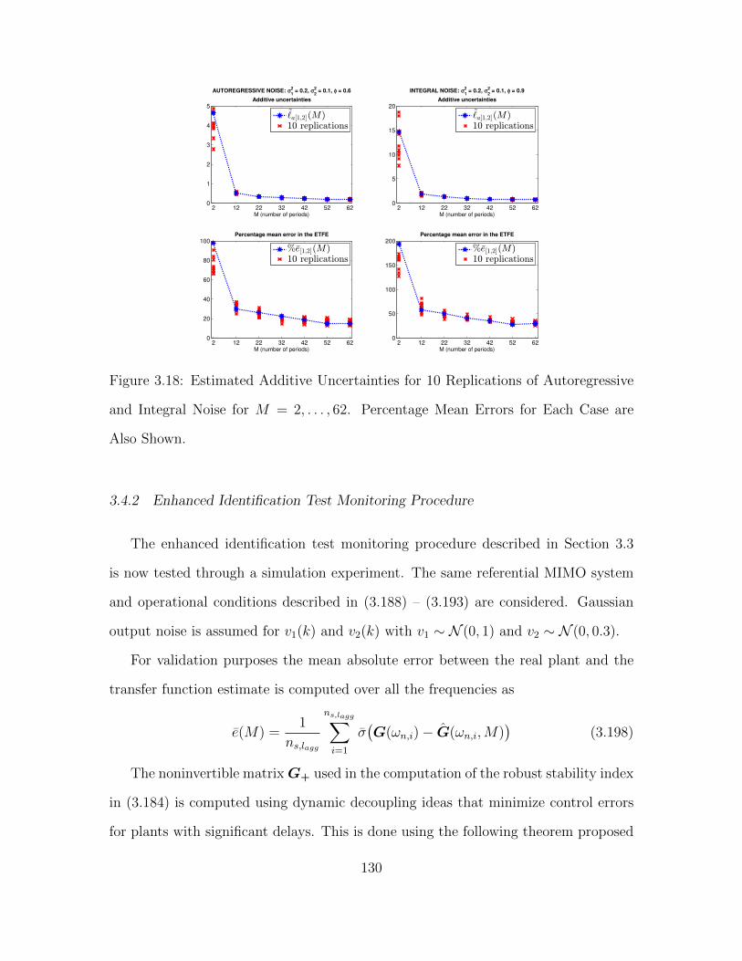
2 12 22 32 42 52 620

1

2

3

4

5


AUTOREGRESSIVE NOISE: σ2

1 = 0.2, σ

2

2 = 0.1, φ = 0.6



2 12 22 32 42 52 620

20

40

60

80

100




2 12 22 32 42 52 620

5

10

15

20


INTEGRAL NOISE: σ2

1 = 0.2, σ

2

2 = 0.1, φ = 0.9



2 12 22 32 42 52 620

50

100

150

200




Figure 3.18: Estimated Additive Uncertainties for 10 Replications of Autoregressive

and Integral Noise for M = 2, . . . , 62. Percentage Mean Errors for Each Case are

Also Shown.

3.4.2 Enhanced Identification Test Monitoring Procedure

The enhanced identification test monitoring procedure described in Section 3.3

is now tested through a simulation experiment. The same referential MIMO system

and operational conditions described in (3.188) – (3.193) are considered. Gaussian

output noise is assumed for v1(k) and v2(k) with v1 ∼ N (0, 1) and v2 ∼ N (0, 0.3).

For validation purposes the mean absolute error between the real plant and the

transfer function estimate is computed over all the frequencies as

e(M) =1

ns,lagg

ns,lagg∑i=1

σ(G(ωn,i)− G(ωn,i,M)

)(3.198)

The noninvertible matrixG+ used in the computation of the robust stability index

in (3.184) is computed using dynamic decoupling ideas that minimize control errors

for plants with significant delays. This is done using the following theorem proposed

130

by Holt and Morari (1985):

Theorem 1 The diagonal Gd+ matrix with the smallest delay terms such that the

multivariable IMC controller Q = G−1− = G−1G+ is realizable has the form

Gd+ = diag(rii, · · · , rjj, · · · , rnn) (3.199)

where

rjj = e−smaxi

(max(

0,(qij−pij)))

(3.200)

and pij is the minimum delay in the numerator of element ij of G−1, and qij is the

minimum delay in the denominator of element ij of G−1.

Using Theorem 1 with the model described in (3.188), and assuming that a priori

information about the delays is available, the resultant matrix and filter are

G+ =

e−27s 0

0 e−14s

, F =

1λ1s+1

0

0 1λ2s+1

(3.201)

The maximum robust stability indexes among all frequencies for each cycle are

computed as

RPimax(M) = maxωn,i∈Wn,lagg

RPi(ωn,i,M) (3.202)

To find the values for the parameters λ1 and λ2 according to (3.187) a simple exhaus-

tive search is performed varying each λi from 10 to 100 with increments of 2 units,

and then finding the values of λ∗1 and λ∗2 that combined result in the minimum value

for RPimax(M). An example of the proposed search process is illustrated in Fig. 3.19.

The performance weighting function wP is defined using (3.178) considering AP =

10−3 and MP = 2. By observing the defined asymptotic frequency bands in Fig. 3.10,

131

100

80

60

61

40

20

3D plot

00

20

40

62

60

80

1.8

1.9

1.2

1.3

1.1

1.4

1.5

1.6

1.7

100

RP

i ma

x

Contour plot

61

10 20 30 40 50 60 70 80 90 100

62

10

20

30

40

50

60

70

80

90

100

Minimum point: 61

*=68, 6

2

*=82

Figure 3.19: Illustration of the Proposed Simple Search Procedure for the Values λ∗1

and λ∗2 That Minimizes RPiMax.

and considering again the dominant time constant of τdom = 60 then

MPωb ≈1

τdom, ωb =

1

MP τdom= 0.0083 (3.203)

The simulation is performed, input-output data is analyzed, uncertainty bounds

are computed with ρ = 0.05, and κ = 0.1855 giving a confidence level of 81.45% using

(3.159) for the MIMO estimate. Two different simulation studies are performed and

contrasted to evaluate the “zippered” and full spectral input signal design structures.

3.4.2.1 Simulation Results Using “Zippered” Signals

The “zippered” input signal design procedure described in Section 3.3.2.1 is ap-

plied. Fig. 3.20 illustrates the resulting input and output signals for M = 2 cycles.

Uncertainty computations are performed using the transient LPM, assuming R =

132

Time(min)

0 500 1000 1500 2000 2500 3000 3500 4000

y1

-5

0

5

Time(min)

0 500 1000 1500 2000 2500 3000 3500 4000

y2

-5

0

5

Time(min)

0 500 1000 1500 2000 2500 3000 3500 4000

u1

-0.5

0

0.5

Time(min)

0 500 1000 1500 2000 2500 3000 3500 4000

u2

-0.5

0

0.5

Figure 3.20: Simulation of Input Signals Designed With the “Zippered” Method and

the Resulting Output Signals for M = 2 Cycles With σ21 = 1 and σ2

2 = 0.3.

Real

-2 -1 0 1 2 3 4 5

Imag

-4

-3

-2

-1

0

1

2

G[1;1]

Real

-1.5 -1 -0.5 0 0.5 1 1.5 2

Imag

-2

-1.5

-1

-0.5

0

0.5

1

G[1;2]

Real

-2 -1 0 1 2 3 4 5 6

Imag

-4

-3

-2

-1

0

1

G[2;1]

Real

-2 -1 0 1 2 3 4 5 6

Imag

-4

-3

-2

-1

0

1

G[2;2]

Real plant

Additive uncertainty region

100 replications

Figure 3.21: Additive Uncertainties for the “Zippered” Design Drawn as Circular

Regions Around Each Real Transfer Function Response, Showing Different Transfer

Function Estimates for 100 Realizations of the Same Gaussian Noise.

133

2, and nT = 6 resulting in dfT = 5. Fig. 3.21 illustrates the computed additive

uncertainty regions drawn as circles around the real values of the transfer functions.

New estimates of the transfer functions for each frequency are also presented using

100 different realizations of the same type of noise.

Results for a maximum of M = 16 periods of the same input signals with no

modifications are shown in Fig. 3.22. The upper plot shows results for the robust

performance test while the lower plot shows a validation perspective through the

computation of the mean error. The proposed stopping criterion described in (3.185)

is evaluated considering nMi = 2 consecutive iterations. It can be observed that the

desired conditions are met, and the experiment can be stopped after M = 11 periods

with a total length of 22528 minutes. The mean error at that point is e(11) = 0.31

what represents a reduction of 48% compared to the error estimate at M = 2 cycles.

Different types of modifications in the input signals are tested. Fig. 3.23 and

Fig. 3.24 present simulation results including changes on the amplitude and the fun-

damental frequency of the inputs signals for M = 3 cycles.

Results for the monitoring procedure are shown in Fig. 3.25 where the dotted line

represents increments on the amplitude of the signals after M = 6 cycles considering

umin1 = umin2 = −1, and umax1 = umax2 = 1. If the same stopping criterion is considered,

the test is now accomplished earlier and the experiment can be stopped after M = 8

cycles with a total duration of 16384 minutes. This type of modification assumes

that the amplitude operational constraints of the signals have not been reached yet.

The dashed line in Fig. 3.25 represents a change on the frequency harmonic content

of the input signals after M = 6 cycles, considering a harmonic step reduction of

Sh,l = 1. If the stopping criterion is evaluated again, the experiment can be halted

after M = 9 cycles with a total duration of 18432 minutes. The type of modification in

134

Number of cycles M

2 3 4 5 6 7 8 9 10 11 12 13 14 15 160.8

1

1.2

1.4

1.6Robust performance test

RPimax(M )Test bound

Number of cycles M

2 3 4 5 6 7 8 9 10 11 12 13 14 15 160.2

0.3

0.4

0.5

0.6

0.7Mean error

7e(M )

Stopping point

Figure 3.22: Illustration of the Monitoring Process for M = 1, · · · , 16 Cycles of the

Same Input Signals With no Modifications. Uncertainties and Robust Performance

Indexes Are Computed for ρ = 0.05

Time(min)

0 1000 2000 3000 4000 5000 6000

y1

-5

0

5

Time(min)

0 1000 2000 3000 4000 5000 6000

y2

-5

0

5

Time(min)

0 1000 2000 3000 4000 5000 6000

u1

-1

0

1

Time(min)

0 1000 2000 3000 4000 5000 6000

u2

-1

0

1

Figure 3.23: Simulation of the “Zippered” Experiment Considering a Total of M = 3

Cycles, and Including a Change on the Input Amplitude After M = 2 Cycles.

135

Time(min)

0 1000 2000 3000 4000 5000 6000

y1

-5

0

5

Time(min)

0 1000 2000 3000 4000 5000 6000

y2

-5

0

5

Time(min)

0 1000 2000 3000 4000 5000 6000

u1

-0.5

0

0.5

Time(min)

0 1000 2000 3000 4000 5000 6000

u2

-0.5

0

0.5

Figure 3.24: Simulation of the “Zippered” Experiment Considering a Total of M = 3

Cycles, and Including a Change on the Fundamental Frequency of the Inputs After

M = 2 Cycles.

the input signals depends on the available resources and user preferences; however all

modifications lead to improvements in the useful for identification of the experiment.

The performance of the proposed monitoring process is tested through the appli-

cation of 10 independent realizations of the same Gaussian noise with v1 ∼ N (0, 1)

and v2 ∼ N (0, 0.3). Results are shown in Fig. 3.26 where each simulation exhibits in-

formation regarding the robust stability test and validation through the computation

of the mean error when only the number of cycles is increased.

Fig. 3.27 depicts results using an autoregressive noise structure represented by

vn(k) = φvn(k − 1) + at, at ∼ N (0, σ2n) (3.204)

The left-side plots represent a full autoregressive structure considering φ = 0.6, σ21 =

0.2, and σ22 = 0.1. The right-side plots represent a more integral noise action with

a higher autoregressive factor of φ = 0.9 , σ21 = 0.2, and σ2

2 = 0.1. As expected the

136

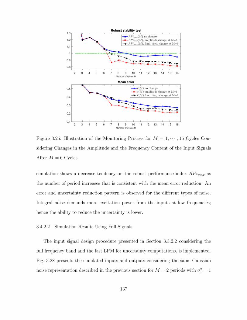
Number of cycles M

2 3 4 5 6 7 8 9 10 11 12 13 14 15 16

0.8

0.9

1

1.1

1.2

1.3Robust stability test

RPimax(M ) no changes

RPimax(M ), amplitude change at M=6

RPimax(M ), fund. freq. change at M=6

Number of cycles M

2 3 4 5 6 7 8 9 10 11 12 13 14 15 160.1

0.2

0.3

0.4

0.5

Mean error

7e(M ) no changes

7e(M ) amplitude change at M=6

7e(M ) fund. freq. change at M=6

Figure 3.25: Illustration of the Monitoring Process for M = 1, · · · , 16 Cycles Con-

sidering Changes in the Amplitude and the Frequency Content of the Input Signals

After M = 6 Cycles.

simulation shows a decrease tendency on the robust performance index RPimax as

the number of period increases that is consistent with the mean error reduction. An

error and uncertainty reduction pattern is observed for the different types of noise.

Integral noise demands more excitation power from the inputs at low frequencies;

hence the ability to reduce the uncertainty is lower.

3.4.2.2 Simulation Results Using Full Signals

The input signal design procedure presented in Section 3.3.2.2 considering the

full frequency band and the fast LPM for uncertainty computations, is implemented.

Fig. 3.28 presents the simulated inputs and outputs considering the same Gaussian

noise representation described in the previous section for M = 2 periods with σ21 = 1

137

Number of cycles

2 3 4 5 6 7 8 9 10 11 12 13 14 15 160.5

1

1.5

2

2.5

3

10 realizations of RPimax

Test bound

Number of cycles

2 3 4 5 6 7 8 9 10 11 12 13 14 15 160.2

0.3

0.4

0.5

0.6

0.7

0.8

10 realizations of 7e(M )

Figure 3.26: Ten Computations of the Robust Performance Index and the Absolute

Mean Error Relying on the “Zippered” Design Generated From Different Realizations

of Gaussian Noise With σ21 = 1, and σ2

2 = 0.3.

and σ22 = 0.3. Uncertainty computations are performed using the fast LPM approach,

considering R = 2, nT = 4, and dfT = 5 for the non-excited frequencies, and R = 3,

nG = 6, and dfG = 5 for the excited frequencies. Fig. 3.29 illustrates the computed

additive uncertainties drawn as circular regions over a Nyquist plot and including

100 replications utilizing the same noise structure but with different realizations for

M = 11 cycles. Considerable bias and higher variability, especially at the border

frequencies can be observed as expected. To avoid problems due the border effect

described in Section 3.3.1.3, the uncertainties computed for the two shorter and the

two higher frequencies in the grid are neglected as is illustrated in Fig. 3.30.

The monitoring process is performed and results for a maximum of M = 16 cycles

are shown in Fig. 3.31, where the upper plot again represents the robust performance

index contrasted with test bound presented in (3.185). The lower plot presents vali-

138

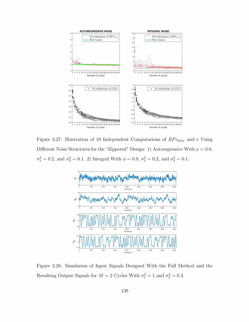
Number of cycles

2 4 6 8 10 12 14 16 18 20 22 24 26 28 30 32 34 36 38 400

1

2

3

4

5

6AUTOREGRESSIVE NOISE


Test bound

Number of cycles

2 4 6 8 10 12 14 16 18 20 22 24 26 28 30 32 34 36 38 400.2

0.3

0.4

0.5

0.6

0.7

0.8

0.9

10 realizations of 7e(M)

Number of cycles

2 4 6 8 10 12 14 16 18 20 22 24 26 28 30 32 34 36 38 400

2

4

6

8

10

12

14

16INTEGRAL NOISE


Test bound

Number of cycles

2 4 6 8 10 12 14 16 18 20 22 24 26 28 30 32 34 36 38 400.2

0.4

0.6

0.8

1

1.2

1.4

1.6

1.8

2


Figure 3.27: Illustration of 10 Independent Computations of RPiMax and e Using

Different Noise Structures for the “Zippered” Design: 1) Autoregressive With φ = 0.6,

σ21 = 0.2, and σ2

2 = 0.1. 2) Integral With φ = 0.9, σ21 = 0.2, and σ2

2 = 0.1.

Time(min)

0 500 1000 1500 2000 2500 3000 3500 4000

y1

-5

0

5

Time(min)

0 500 1000 1500 2000 2500 3000 3500 4000

y2

-5

0

5

Time(min)

0 500 1000 1500 2000 2500 3000 3500 4000

u1

-0.5

0

0.5

Time(min)

0 500 1000 1500 2000 2500 3000 3500 4000

u2

-0.5

0

0.5

Figure 3.28: Simulation of Input Signals Designed With the Full Method and the

Resulting Output Signals for M = 2 Cycles With σ21 = 1 and σ2

2 = 0.3.

139

Real

-3 -2 -1 0 1 2 3 4 5

Imag

-4

-3

-2

-1

0

1

2

3

G[1;1]

Real

-3 -2 -1 0 1 2 3

Imag

-2

-1

0

1

2

3

G[1;2]

Real

-4 -2 0 2 4 6

Imag

-4

-3

-2

-1

0

1

2

G[2;1]

Real

-4 -2 0 2 4 6 8

Imag

-4

-3

-2

-1

0

1

2

G[2;2]

Real plant


100 replications

Figure 3.29: Additive Uncertainties for the Full Design Drawn As Circular Regions

Around Each Real Transfer Function Response, Showing Different Transfer Function

Estimates for 100 Realizations of the Same Gaussian Noise.

dation results through the computation of the absolute mean error using (3.198). It

can be observed that using the proposed stopping criterion considering accomplish-

ment of the test for nMi = 2 consecutive iterations, the experiment can be halted

after M = 12 iterations with a total duration of 24576 minutes, and a mean error

of e(12) = 0.314. The same experiment is repeated utilizing 10 different realizations

of the same Gaussian noise; results are presented in Fig. 3.32 where the reduction

tendency can be observed with higher variability. The different types of input signal

modifications are again tested for the full design, including changes on the amplitude

and the fundamental frequency content. Results are presented in Fig. 3.33 depicting

changes in the amplitude of the input signals to umin1 = umin2 = −1, umax1 = umax2 = 1,

and a harmonic step reduction to Sh,l = 1. Best results in both the robust perfor-

140

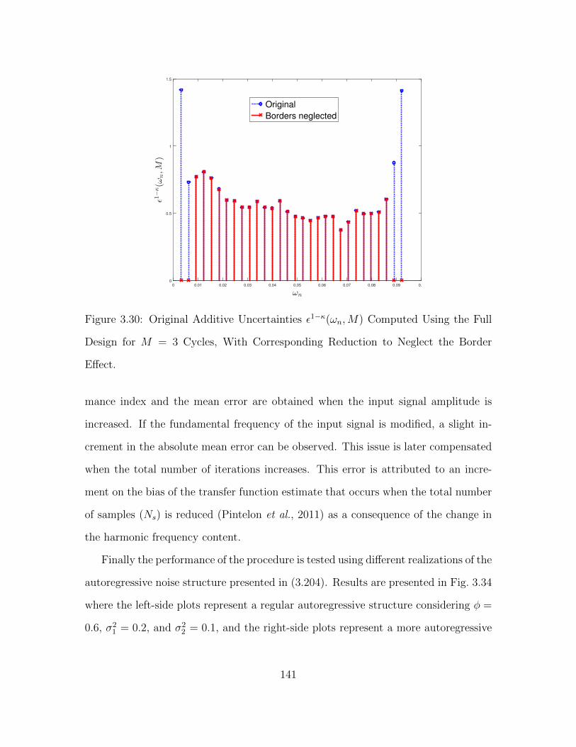
!n

0 0.01 0.02 0.03 0.04 0.05 0.06 0.07 0.08 0.09 0.1

01!5(!

n;M

)

0

0.5

1

1.5

Original

Borders neglected

Figure 3.30: Original Additive Uncertainties ε1−κ(ωn,M) Computed Using the Full

Design for M = 3 Cycles, With Corresponding Reduction to Neglect the Border

Effect.

mance index and the mean error are obtained when the input signal amplitude is

increased. If the fundamental frequency of the input signal is modified, a slight in-

crement in the absolute mean error can be observed. This issue is later compensated

when the total number of iterations increases. This error is attributed to an incre-

ment on the bias of the transfer function estimate that occurs when the total number

of samples (Ns) is reduced (Pintelon et al., 2011) as a consequence of the change in

the harmonic frequency content.

Finally the performance of the procedure is tested using different realizations of the

autoregressive noise structure presented in (3.204). Results are presented in Fig. 3.34

where the left-side plots represent a regular autoregressive structure considering φ =

0.6, σ21 = 0.2, and σ2

2 = 0.1, and the right-side plots represent a more autoregressive

141

Number of cycles M

2 3 4 5 6 7 8 9 10 11 12 13 14 15 160.9

1

1.1


RPimax(M )Test bound

Number of cycles M

2 3 4 5 6 7 8 9 10 11 12 13 14 15 160.3

0.4

0.5

0.6

0.7Mean error

7e(M )

Stopping point

Figure 3.31: Illustration of the Monitoring Process for M = 1, · · · , 16 Cycles of the

Same Input Signals With No Modifications. Uncertainties and Robust Performance

Indexes Are Computed for ρ = 0.05.

Number of cycles

2 3 4 5 6 7 8 9 10 11 12 13 14 15 160.5

1

1.5

2

2.5

3

3.5


Test bound

Number of cycles

2 3 4 5 6 7 8 9 10 11 12 13 14 15 160.2

0.3

0.4

0.5

0.6

0.7

0.8

10 realizations of 7e(M )

Figure 3.32: Ten Computations of the Robust Performance Index and the Absolute

Mean Error Relying on the Full Design Generated From Different Realizations of

Gaussian Noise With σ21 = 1, and σ2

2 = 0.3.

142

2 3 4 5 6 7 8 9 10 11 12 13 14 15 16

0.8

0.9

1

1.1

1.2

1.3

RPimax(M ) no changes

RPimax(M ), amplitude change at M=6

RPimax(M ), fund. freq. change at M=6

2 3 4 5 6 7 8 9 10 11 12 13 14 15 160.2

0.25

0.3

0.35

0.4

0.45

0.5

0.55

7e(M ) no changes

7e(M ) amplitude change at M=6

7e(M ) fund. freq. change at M=6

Number of cycles M (top scale : original and amp. change / bottom scale : change in fund. freq.)

2 3 4 5 6 7 8 9 10 11 12 13 14 15 16 17 18 19 20 21 22 23 24 25 26

Number of cycles M (top scale : original and amp. change / bottom scale : change in fund. freq.)

2 3 4 5 6 7 8 9 10 11 12 13 14 15 16 17 18 19 20 21 22 23 24 25 26

Figure 3.33: Illustration of the Monitoring Process for M = 1, · · · , 16 Cycles Con-

sidering Changes in the Amplitude and the Frequency Content of the Input Signals

After M = 6 Cycles.

Number of cycles

2 4 6 8 10 12 14 16 18 20 22 24 26 28 30 32 34 36 38 400.5

1

1.5

2

2.5



Test bound

Number of cycles

2 4 6 8 10 12 14 16 18 20 22 24 26 28 30 32 34 36 38 400.2

0.3

0.4

0.5

0.6

0.7

0.8

0.9


Number of cycles

2 4 6 8 10 12 14 16 18 20 22 24 26 28 30 32 34 36 38 400

5

10

15INTEGRAL NOISE


Test bound

Number of cycles

2 4 6 8 10 12 14 16 18 20 22 24 26 28 30 32 34 36 38 400.2

0.4

0.6

0.8

1

1.2

1.4

1.6

1.8

2


Figure 3.34: Illustration of 10 Independent Computations of RPiMax and e Using

Different Noise Structures for the Full Design: 1) Autoregressive With φ = 0.6,

σ21 = 0.2, and σ2

2 = 0.1. 2) Integral With φ = 0.9, σ21 = 0.2, and σ2

2 = 0.1.

143

(integrative) noise action with φ = 0.9 , σ21 = 0.2, and σ2

2 = 0.1. For the regular

autoregressive case it can be observed that the test bound is accomplished in most

of the cases after 25 cycles with a considerable reduction in the mean error. For the

integral case there is a reduction in the error and in the performance index, however

the test conditions are hardly barely satisfied. A modification of performance weights

or a relaxation on the test conditions may be needed.

3.5 Chapter Summary

This chapter presents an identification test monitoring procedure that determines

the shortest possible experiment in terms of the problem definitions (e.g., Ns, ns), and

at the same time with data that is sufficiently informative for identification purposes.

Different formulations of the problem are presented and contrasted.

A basic approach that assumes data measured at steady state is initially pre-

sented. Simulations show that bounds BAV , BRV , and nMi cannot be rigidly defined;

user intervention is important for their adjustment in real time. Because of the mul-

tivariable nature of the system and the use of “zippered” power spectrums, the total

duration of the experiment N is affected by the number of inputs nu as was shown

in (3.10); however the same dependence would have existed, if nu independent SIMO

experiments had been designed instead. The uncertainty computation method can be

applied to different situations where no a priori knowledge of the noise structure is

available, and also when the input signal is not designed by the user but is periodic in

nature and can be measured. Multivariable uncertainty computation leads to results

that are valid for all the input/output elements. In practical applications and for

identification purposes the worst case scenario criterion may give acceptable results,

as the simulation results suggest. The disadvantage of the basic method is that it

requires output signals measured at steady state to account for transient responses;

144

hence no modifications can be performed to the input signals during the experimental

execution.

An enhanced identification test monitoring methodology was also proposed. An

evaluation is accomplished after each input period, from which three possible actions

are proposed: increasing the length of the experiment (by adding another cycle), in-

creasing the amplitude of the signal, or adjusting the frequency content of excitation

in the signal. To account for the transient effect caused by these modifications, the

Local Polynomial Method (LPM) was adopted for the transfer function and uncer-

tainty computation. Two variants of the LPM were tested, first the transient LPM

using “zippered” multisine input signals, and the fast LPM method using input sig-

nals defined for the full frequency band of interest. There is a trade between these

approaches: the zippered design offers a less conservative and more accurate definition

of uncertainties and robust performance index, while the full method offers a better

frequency resolution and hence possible smaller time intervals. Simulations proved

that the “zippered” design exhibits a better performance in terms of bias error and

variability of the estimation. The experiment ends when a predefined criterion based

on robust performance metrics is satisfied.

Simulations demonstrated the ability of the identification test monitoring proce-

dure to identify an appropriate moment to halt the experiment. Increasing the am-

plitude of the input signal is a effective means for improving the experiment; however

because of operational constraints this is not always possible. A second alternative is

to modify how power is distributed over frequency in the input signal, increasing its

contribution at some frequencies while keeping the total power constant. This was

accomplished in the paper by redistributing harmonic excitation content. Ultimately,

the decision to take after each evaluation point will depend on operational constraints

and user preferences.

145

Chapter 4

DESIGN OF OPEN-LOOP BEHAVIORAL INTERVENTIONS RELYING ON

SYSTEM IDENTIFICATION IDEAS

4.1 Overview

As noted in Chapter 1, physical inactivity is a serious behavioral problem that

contributes to a high number of mortalities in the U.S. each year (Mokdad et al.,

2004). The use of emerging technologies, such as smartphones and wearable sensors,

is enabling the application of novel mobile and wireless (mHealth) interventions (Hek-

ler et al., 2013b) that lend themselves to a systematic and mathematically rigorous

approach. The results are interventions that rely on highly intensive measurement

of outcomes of interest to make decisions on intervention treatment components and

dosages that are opportunely delivered; hence these interventions are referred to in

the literature as Intensively Adaptive Interventions (IAI; Riley et al. (2015b)).

In order to design optimal interventions through the use of effective feedback

(and/or feedforward) controllers, it is necessary to obtain an adequate model that

properly represents the dynamical nature of the system. As noted in Chapter 2, Social

Cognitive Theory (SCT) (Bandura, 1977, 1986) is a highly prevalent and generally

well-regarded conceptual framework within behavioral science that has been used to

design a variety of behavioral interventions. The developed dynamical model of SCT

will be used to represent the dynamic nature of the low physical activity behavioral

problem.

In this work, the term “plant” refers to a human behavioral system defined as a dy-

namical model based on SCT. IAIs can address the problem of low physical activity in

146

sedentary individuals, using SCT as the conceptual framework. If these interventions

are to be based on control systems engineering principles, then an appropriate esti-

mation of the behavioral dynamics should be obtained first. A semi-physical system

identification procedure is proposed to search and refine the individual SCT model

parameters. One important goal of the experimental input design is to satisfy iden-

tification requirements such as persistent excitation and at the same time keep the

variations within user-defined, “patient-friendly” (Deshpande et al., 2012) constraints.

An additional challenge in behavioral intervention settings is to obtain outputs that

are consistent with the goals and the practical demands of the intervention.

In this chapter an input signal design will be proposed, together with an estima-

tion procedure, that provides an adequate plant model and at the same time enables

accomplishing desired behavioral outcomes during the course of the experiment. The

proposed strategy will consider the construction of two open-loop experiments with

different inputs. The first one is referred to as an informative experiment. It is de-

signed based on a priori knowledge from behavior change theory and previous expe-

rience with behavioral interventions. This experiment will provide basic preliminary

information on the dynamics of the system and lead to an initial model.

Two different alternatives for the informative experiment will be presented; the

first one relies on random signals generated within user-defined bounds, with the goal

to achieve the required amount of daily steps per week (e.g., 10,000). The second

alternative will propose a design procedure with the shortest possible duration, that

correspondingly allows inferring the important dynamical properties of the system.

This will be done using the approach presented in Chapter 3 testing both, the basic

and enhanced identification test monitoring methods. This result has important

practical implications in behavioral interventions, given that systematic approaches

for determining experimental duration in single-subject /“idiographic” experiments

147

are not well-understood. Under the assumption that noise in the signals is the major

source of uncertainty in the estimation, a deterministic periodic input signal can be

employed to analyze and extract frequency domain information that can be used

in the computation of probabilistic uncertainty descriptions. In the basic method

the required uncertainty bounds are estimated relying on a non-parametric averaged

Empirical Transfer Function Estimates (ETFE). The enhanced approach relies on the

Local Polynomial Method (LPM) to compute transfer functions and uncertainties,

allowing the incorporation of changes in the amplitude or the frequency content of

the input signals. To obtain independent computations of each input-output transfer

function of the MIMO system for both methods, the input design will consider a

multisinusoidal “zippered” spectra (Rivera et al., 2009) and will include a “patient-

friendly” selection of phases.

The second experiment is an optimized experiment that will use the results from

the informative experiment, to shape the behavioral outcomes to a desired pattern. It

is designed by solving a formal optimization problem that searches for the best inputs,

considering the estimated preliminary model and expected performance requirements.

Both experimental designs will consider internal logic conditions that are present in

a behavioral situation, and will be properly specified.

The chapter is organized as follows: Section 4.2 presents a description of the com-

ponents and decision algorithms that form part of the physical activity intervention.

It also describes general design constraints, and details about the proposed grey-box

estimation. Section 4.3 describes the design of the informative experiment, including

input signal generation through pseudo-random signals and using an identification

test monitoring procedure. Section 4.4 explore the design of the optimized experi-

ment as a constrained optimization problem. Section 4.5 shows a simulation study

and results using the proposed procedure. Section 4.6 gives summary and conclusions

148

of the chapter.

4.2 Description of the Physical Activity Intervention and the System Identification

Problem

The main purpose of the intervention is to promote physical activity, e.g., walk-

ing/running, among inactive adults age 21 years and older, with a specific goal of

reaching 10,000 steps per day on average per week. Social Cognitive Theory (SCT;

Bandura (1986)) can be used to represent this problem. SCT is an extensively used

conceptual and theoretical framework for behavioral interventions, including physical

activity (Bandura, 1998).

4.2.1 Simplified SCT Model

In Chapter 2, a dynamical interpretation of SCT was developed, based on a fluid

analogy that describes the interrelationships among psychosocial variables. SCT de-

scribes a human agency perspective of behavior (η4) in which individuals proactively

self-reflect, self-regulate, and self-organize (Bandura, 1989). The intervention is fo-

cused on one of the internal loops within the SCT model, that represents a “behavior-

ist” articulation of the determinants of behavior (Ferster, 1970; Baum, 2011). This is

depicted in Fig. 4.1, through a simplified version of the SCT model where coefficients

ξi represent the main inputs, ηi are the outputs, γij and βij represent the interrelation

among the different constructs, ζi are external disturbances, and θi are delay times.

For the simplified version of the SCT model, applied to the physical activity prob-

lem, the most important constructs include behavior (η4) that is the action of interest

(e.g., amount of performed daily steps), outcome expectancy (η2) that is the perceived

likelihood that performing a given behavior will result in certain behavioral outcomes

(η5) (e.g., weight reduction); these outcomes are greatly influenced by the environ-

149

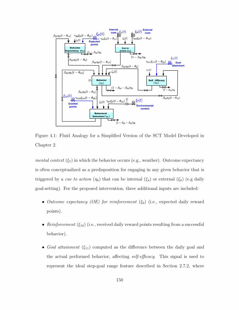
Outcome

Expectancy ( )

Behavior

Behavioral

Outcomes

γ64ξ4(t − θ11)

Cue to

action ( )

γ57ξ7(t − θ15)

ξ4(t)

ξ7(t)

ζ2(t)

ζ4(t)

ζ5(t)

β42η2(t − θ6)

β54η4(t − θ12)

β25η5(t − θ14)

(1 − β54 − β34)η4

(1 − β42)η2

(1 − β25 − β45)η5

η2

(η4)

(η5)

ξ8(t)

γ68ξ8(t − θ18)ζ6(t)

(1 − β46)η6

β46η6(t − θ17)

η6

Fγ510ξ10(t − θ20)

β45η5(t − θ19)

γ29ξ9(t − θ21)

LT

Expected

points

Granted

points

ξ9(t)

ξ10(t)

Self - Efficacy

ζ3(t)

β34η4(t − θ13)

β43η3(t − θ8)

(1 − β43)η3

(η3)

γ311ξ11(t − θ22)ξ11(t)

Goal

attainment

Environmental

context

Internal

cuesExternal

cues

Figure 4.1: Fluid Analogy for a Simplified Version of the SCT Model Developed in

Chapter 2.

mental context (ξ7) in which the behavior occurs (e.g., weather). Outcome expectancy

is often conceptualized as a predisposition for engaging in any given behavior that is

triggered by a cue to action (η6) that can be internal (ξ4) or external (ξ8) (e.g daily

goal-setting). For the proposed intervention, three additional inputs are included:

• Outcome expectancy (OE) for reinforcement (ξ9) (i.e., expected daily reward

points).

• Reinforcement (ξ10) (i.e., received daily reward points resulting from a successful

behavior).

• Goal attainment (ξ11) computed as the difference between the daily goal and

the actual performed behavior, affecting self-efficacy. This signal is used to

represent the ideal step-goal range feature described in Section 2.7.2, where

150

individuals might react negatively to too high a goal that they consider difficult

to reach.

Based on the described analogy and assuming first-order dynamics for each inven-

tory, the following equations for the simplified SCT model are developed:

τ2dη2

dt= γ29ξ9(t− θ21) + β25η5(t− θ14)− η2(t) + ζ2(t) (4.1)

τ3dη3

dt= γ311ξ11(t− θ22) + β34η4(t− θ13)− η3(t) + ζ3(t) (4.2)

τ4dη4

dt=β42η2(t− θ6) + β43η3(t− θ8) + β46η6(t− θ17) + β45η5(t− θ19)

− η4(t) + ζ4(t)

(4.3)

τ5dη5

dt= γ57ξ7(t− θ15) + γ510ξ10(t− θ20) + β54η4(t− θ12)− η5(t) + ζ5(t) (4.4)

τ6dη6

dt= γ64ξ4(t− θ11) + γ68ξ8(t− θ18)− η6(t) + ζ6(t) (4.5)

As was described in Chapter 2, it is possible (based on data or prior knowledge) to

use higher-order differential equations to describe the behavior, or to add nonlinear

features (such as habituation).

IAI components can be delivered by decision algorithms (i.e., controllers) to influ-

ence behavior and, consequently, the other SCT constructs. The goal in this chapter is

to formulate an intervention that can be designed beforehand in an open-loop setting

for identification purposes.

4.2.2 Intervention Components

In order to design effective intervention controllers, a “sufficiently good”/adequate

plant model is required. Since the main hypothesis of this work is that physical

activity interventions can be represented through SCT, the use of a dynamical model

per Section 4.2 as a priori structural information is assumed. Fig. 4.2 depicts the

interaction of the open-loop intervention over the simplified SCT model through the

151

following components:

η4

ξ4

ξ9

ξ10

Simplified

SCT

Model

ξ7

Goals

Intervention


Desireddaily steps

u8

Expected points

If / Then

Grantedpoints

u9

u10 Behavioral outcomes

Behavior (steps)

η5

y4+

_

ξ11

Goalattainment

u11

Self-efficacyη3

Outcome expectancy

η2

Steps self-regulatorvia internal cues

+

_

csr

u7

Figure 4.2: Conceptual Diagram for the Proposed Intervention to Influence Behav-

ior and Other Constructs Represented by the Simplified SCT Model. Input/output

Symbols ξi and ηi are Used for Modeling and Simulation, While ui and yi are Used

for Formulations of the Informative and Optimized Experiments.

• Daily goals (u8), to establish the desired amount of daily steps (e.g., 10,000).

• Expected points (u9), as an outcome expectancy for reinforcement (ξ9) that lets

the participant know the daily expected reward points.

• Granted points (u10), as a reinforcement (ξ10) through an “If/Then” block that

delivers the announced expected points (u10 = u9) only if the performed steps

(y4) are greater or equal than the specified goal (u8).

The intervention is implemented using an SCT model enhanced with individual-

ized self-regulation via internalized cues. In the work of Carver and Scheier (1998)

self-regulation mechanisms for human behavior are expressed as feedback control sys-

tems, where individuals take self-corrective adjustments to stay on track for a defined

goal. To represent self-regulation process we rely on a controller that makes adjust-

ments to internal cues (ξ4) based on the discrepancies between the set goal (u8) and

152

the measured outcome (y4). The controller must allow for a partial level of setpoint

tracking that allows the rest of the intervention components (e.g., points) to also in-

fluence for changes in the output. Internal model control (IMC; Morari and Zafiriou

(1989)) is used to formulate a self-regulator via internalized cues relying on the trans-

fer function p44 from input ξ4 to output η4 computed from the SCT model. Fig. 4.3

is the block diagram representing the IMC design structure, where p44 is the plant,

p44 is the nominal model, d is an external disturbance, pd is the disturbance model,

and qsr is the self-regulator (expressed in q-parametrization form).

u8 y4p44qsr+

++

+

p44

pd

ξ4 η4

d

_Goals Steps

Feedback controller csr

+

Figure 4.3: Block Diagram Representing the IMC Design Structure for the Self-

Regulator Via Internalized Cues.

The closed-loop relationships between variables in Fig. 4.3 are given by

y4 =p44qsr

1 + (p44 − p44)qsru8 +

(1− p44qsr)pd1 + (p44 − p44)qsr

d (4.6)

ξ4 =qsr

1 + (p44 − p44)qsru8 −

pdqsr1 + (p44 − p44)qsr

d (4.7)

In the absence of plant-model mismatch (p44 = p44) these reduce to

y4 = p44qsru8 + (1− p44qsr)pdd (4.8)

ξ4 = qsru8 − pdqsrd (4.9)

153

Assuming that the dominant effect on the output is obtained from the time constant

of the behavior inventory (τ4), the nominal model is considered as

p44 =β46γ64

τ4s+ 1≈ η4

ξ4

(4.10)

It is desirable to have a controller that makes the process output follow its setpoint

and reject all disturbances. According to the IMC formulation, the self-regulator is

defined as

qsr = p−144 fsr = p−1

44

Ksr

λs+ 1(4.11)

where a Type I filter fsr is used to ensure properness of the final control system. The

representation of the self-regulator as a classical feedback controller is

csr =qsr

1− p44qsr=

Ksr

β46γ64

τ4s+ 1

λs+ 1−Ksr

(4.12)

The performance of the self-regulator is characterized by the value of the parameter

λ that reflects the closed-loop speed of response, and the parameter Ksr that ranges

from 0 to 1, with 1 representing perfect integral action.

The proposed intervention considers only variables that are potentially measurable

in a preliminary study, hence internal cues (ξ4), outcome expectancy (η2), and cue

to action (η6) are not considered. Based on previous experimental studies using

smartphones (King et al., 2013; Adams et al., 2013), measurements will be taken daily.

The basic choice of inputs and outputs for identification corresponds to those that

will be used by the intervention as was depicted in Fig. 4.2. The inputs (e.g., goals,

reward points) should be delivered to the participant through the smartphone and

the outputs will also be collected in the phone (e.g., steps via the internal pedometer).

Proper measurement is crucial for success of the identification procedure, and the

following steps must be followed to guarantee reliability of the information: observa-

tional studies, equipment selection, software development, prototyping, test design,

154

among others. In behavioral health, this activity falls under the topic of ecological

momentary assessment (Shiffman et al., 2008).

4.2.3 Grey-Box Parameter Estimation

Parameter estimation is done through semi-physical modeling, a technique that

takes into account physical insight about the system (Lindskog and Ljung, 1995).

In this sense a grey-box parameter estimation procedure (Ljung, 1999) should be

applied, where input-output data from an experiment under real-life circumstances

must be collected. Grey-box parameter estimation relies on two sources of information

to estimate the required model: prior knowledge of the system (in this case the SCT

dynamical model), and experimental data (Lindskog and Ljung, 1995; Bohlin, 1994).

This technique allows the use of a specific state space structure, where the value of a

set of unknown model parameters must be estimated.

To find a state space representation of the system for identification purposes,

differential Equations (4.1) - (4.5) are used together with the representation of the

self-regulator csr that adds a new state referred as η7. Considering only signals from

Fig. 4.2 with no disturbances or delays (ζi = 0, θi = 0, ∀i), the following structure is

obtained:

xp(t) = A(θp)xp(t) +B(θp)up(t) +Ke(t)

yp(t) = Cxp(t) + v(t)

(4.13)

where e and v are uncertainties, xp is the state vector, up the input vector, yp the

output vector and θp is a vector of the unknown model parameters defined as

xp = [η2 η3 η4 η5 η6 η7]> (4.14)

up = [u7 u8 u9 u10]> (4.15)

yp = [y2 y3 y4 y5]> (4.16)

155

θp = [τ2 τ3 τ4 τ5 τ6 β25 β34 β42 β43 β45 β46 β54

γ57 γ64 γ29 γ510 γ311 Ksr λ]> (4.17)

Considering that the goal attainment signal can be represented within the state

space representation via u11 = y4 − u8, the state-space system matrices are

A(θp) =

− 1τ2

0 0 β25

τ20 0

0 − 1τ3

β34+γ311

τ30 0 0

β42

τ4

β43

τ4− 1τ4

β45

τ4

β46

τ40

0 0 β54

τ5− 1τ5

0 0

0 0 −γ64Msrτ4τ6

0 − 1τ6

γ64Msr(1−Nsrτ4)τ6

0 0 −1 0 0 −Nsr

(4.18)

B(θp) =

0 0 γ29

τ20

0 −γ311

τ30 0

0 0 0 0

γ57

τ50 0 γ510

τ5

0 γ64Msrτ4τ6

0 0

0 1 0 0

(4.19)

C =

1 0 0 0 0 0

0 1 0 0 0 0

0 0 1 0 0 0

0 0 0 1 0 0

(4.20)

with Msr =Ksr

γ64β46λ, and Nsr =

1−Ksr

λ.

The actual dimensions of theC matrix depend on the available measurement outputs.

To estimate θp the well-known prediction-error identification methods (PEM; Ljung

156

(1999)) will be used. The one-step ahead prediction error of the system is

ε(t,θp) = yp(t)− yp(t|t− 1,θp) (4.21)

where yp(t|t− 1,θp) is the predicted output based on estimated models.

4.2.4 General Design Constraints

In the ensuing formulations, N ∈ N will be referred as the number of measurements

in days and signals un ∈ RN and ym ∈ RN as vectors containing the design inputs

and outputs respectively, where n and m are the considered input and output indexes.

For input signal design, only a subset of the inputs and outputs used for subsequent

parameter estimation will be considered. The design inputs are goal-setting (u8) and

expected points (ξ9 = u9), Environmental context (ξ7) will not be used because it is

an external variable that, while measurable, cannot be manipulated by the user. The

input design procedure must consider the presence of an “If/Then” decision block as

was depicted in Fig. 4.2, which delivers daily points (i.e., makes ξ10 = u10 = u9) only if

the actual behavior (y4 = η4) meets or exceeds the daily goal (u8). For the optimized

experiment, the main interest is to shape the participant’s “behavior” (y4 = η4).

Therefore, it will be the only output considered in this formulation, however other

outputs are also considered for identification purposes.

Input design must be implemented under strict clinical constraints (also called

“patient friendly”). Therefore, the following general constraints must be considered:

1. Bounds must be imposed on the magnitude of the intervention components

uminn (k) ≤ un(k) ≤ umaxn (k), k = 1, . . . , N (4.22)

where uminn ,umax

n ∈ RN are vectors containing the minimum and maximum

allowed daily value for each input, where in absence of any additional constraint

uminn (k) = Zminn , k = 1, . . . , N (4.23)

157

umaxn (k) = Zmaxn , k = 1, . . . , N (4.24)

2. The inputs are constrained to have a maximum move size MSn that may depend

on the type of intervention

∆un(k) =∣∣un(k)− un(k − 1)

∣∣, k = 2, . . . , N (4.25)

∆un(k) ≤MSn, k = 2, . . . , N (4.26)

3. A minimum switching time Tsw ∈ N can also be imposed to the system to avoid

excessive changes in the intervention components

un(k)− un(k + j) = 0, j = 1, . . . , Tsw − 1

∀k = 1 + l.Tsw, l = 0, 1, ...

k + Tsw − 1 ≤ N

(4.27)

4. In addition, any input un can be constrained for a late start at day Dn as

un(k) = 0, k = 1, . . . , Dn − 1 (4.28)

4.3 Informative Experimental Design

The primary goal of the informative experiment is to gain insights about the basic

dynamics of the system. Two different approaches are tested: first an input signal

design using a randomized signal generation strategy, and a design using deterministic

multisine input signals aimed to the application of identification test monitoring ideas

presented in Chapter 3.

4.3.1 Randomized Signal Generation

Since little is currently known a priori regarding the dynamical system proper-

ties of a physical activity IAI, an initial approach would be to use constrained yet

158

standard input signals (i.e., random, RBS, PRBS, multisine) with sufficient excita-

tion. However, this could cause undesired variations on the participant’s behavior.

Therefore, an initial judicious experiment will be developed; the proposed inputs will

rely on an a priori study (King et al., 2013; Adams et al., 2013), designed to produce

data according to an expected profile, combined with the mentioned standard in-

put signals that will facilitate capturing the dynamical relationships among variables.

The input signals to be designed are goal-setting (u8) and available points (u9), the

signal granted points (u10) will be internally generated by the “if/then” block, as was

described in Fig. 4.2.

Assuming that the individual starts the experiment with an average value of daily

steps called baseline (Bs), the vector goal-setting (u8), will take samples from a

discrete uniform distribution, that represents an increment of 0%, 20%, 40%, 60%,

80% or 100% of Bs, such that

W = {w1, . . . , w6} = {Bs, 1.2Bs, 1.4Bs, 1.6Bs, 1.8Bs, 2Bs} (4.29)

P (u8(k) = wi) =1

6, ,∀wi ∈ W, k = 1, . . . , N (4.30)

where P (·) represents an event probability. The vector available points (u9) will take

a set of random uniform values from 100, 300 or 500 such that

Z = {z1, z2, z3} = {100, 300, 500} (4.31)

P (u9(k) = zi) =1

3, ,∀zi ∈ Z, k = 1, . . . , N (4.32)

The inputs must comply with the constraints described by Equations (4.22) - (4.28).

The randomization of the variables supports the orthogonal delivery of information

required by the identification technique. Having specified these input signals, the

informative experiment must be executed. The collected input-output data will be

used in the grey-box parameter estimation procedure described in Section 4.2.3. As a

159

result, an initial informative model with all the parameter values defined, is obtained

which represents a preliminary version of the system’s model, and forms the basis for

subsequent optimization.

4.3.2 Multisine Signal Generation

A second approach for the design of the informative experiment will attempt to

obtain input signals with the shortest possible duration, and at the same time with

sufficient information for identification purposes. As was described in Chapter 3,

this process relies on uncertainty bounds computations based on transfer function

estimates. It is important to highlight that semi-physical methods (i.e., grey box)

will be still used to identify the SCT model parameters; transfer function estimates

will be used only for uncertainty computations to determine the effect of noise over

the estimation process.

The proposed uncertainty bounds will be calculated using frequency domain meth-

ods, and multisinusoidal signals will be employed. The design procedure was com-

pletely described in Chapter 3, some details are repeated here for clarity. Two of

the presented approaches are adapted for the physical activity intervention: the basic

identification test monitoring method using ETFE, and the enhanced method using

the transient LPM for transfer function computations.

4.3.2.1 Basic Identification Test Monitoring Method

This approach relies on uncertainty computations from transfer function estimates

obtained using the Empirical Transfer Function Estimate (ETFE) method and mul-

tisinusoidal signals with a “zippered” frequency spectrum. Multisine inputs are de-

terministic, periodic signals whose spectrum can be directly specified by the designer.

160

The input un (n = 8, 9) can be described as

un(k) = λn

Ns/2∑j=1

√2α[n,j] cos(ωjkTs + φ[n,j])

ωj = 2πjNsTs

, k = 1, . . . , Ns

(4.33)

where λn is the scaling factor, Ns is the period, Ts is the sampling time. For each

harmonic: α[n,j] is a factor used to specify the relative power of the harmonic, ωj is

the frequency, and φ[n,j] is the phase. Coefficients λn are chosen based on the input

constraints described in (4.22).

Factors α[n,j] are chosen to obtain input signals that are excited orthogonally in

frequency. If nu is the number of design inputs (nu = 2 for this case), and ns is the

total amount of independently excited sinusoids, then the total number of harmonics

is ns and the “zippered” spectrum for each signal un can be constructed by specifying

α[n,j] =

1 if j = nu(i− 1) + (n− 7), for i = 1, 2, . . . ns

0 otherwise

(4.34)

The resulting bound for Ns is

Ns ≥ 2ns (4.35)

The input signals will be repeated for M cycles such that the total duration of the

experiment is Ns M days. The period Ns represents the decision time window for the

monitoring process that is expected to be as short as possible; therefore, the bound

defined in (4.35) can be used to estimate Ns assuming an initial guess for ns. If a

priori information is available about the system dynamics, it can be used to refine the

estimates of ns and Ns as was described in Section 3.2.1. Phases φ will be selected

to minimize the crest factor of the signal using the approach proposed by Guillaume

et al. (1991).

161

Transfer Function and Uncertainty Estimation

The proposed estimation procedure considers a multivariable system subject to

output noise, where the effect of each independent transfer function is given by

y∗(k) = P ∗(q)u∗(k) + v∗(k) (4.36)

where u∗(k) and y∗(k) are any given pair of inputs and outputs, P ∗(q) is the respective

sampled-data transfer function, and v∗(k) is the output noise.

Uncertainty bounds are calculated from an averaged Empirical Transfer Function

Estimate (ETFE). In the work of Bayard (1993), a statistical uncertainty computation

is developed; however it requires a priori knowledge of the noise structure which can

be difficult to obtain in behavioral settings. The uncertainty computation used in this

work (Pintelon and Schoukens, 2012) does not require prior knowledge of the noise

structure. The price to be paid for this flexibility is that the uncertainty bounds are

only valid asymptotically. The conditions for the existence of the averaged ETFE

and the proposed uncertainty bounds are:

• Each true plant P ∗(q) is exponentially stable, linear and time invariant.

• Disturbance v∗(k) can be written as filtered white noise with finite order mo-

ments, and is independent from the input u∗(k) and the output y∗(k).

To obtain the ETFEs it is necessary to represent the individual transfer func-

tions for the identification problem described in section 4.2.2. Fig. 4.4 represents an

equivalent block diagram for the behavioral intervention based on the simplified SCT

model and the proposed self-regulation block considering the design inputs u8, u9,

and assuming that the only measured outputs are y4 and y5. Transfer functions from

each input n to each output m are represented by P[m,n](q).

162

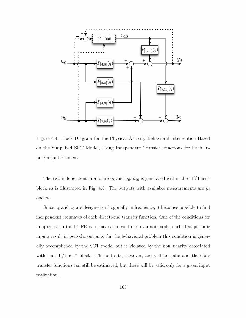
P[4,8](q)

P[5,8](q)

P[4,9](q)

P[5,9](q)

P[4,10](q)

P[5,10](q)

If / Then

++

++

+

+

++

+

u8

u9

y4

y5

u10

Figure 4.4: Block Diagram for the Physical Activity Behavioral Intervention Based

on the Simplified SCT Model, Using Independent Transfer Functions for Each In-

put/output Element.

The two independent inputs are u8 and u9; u10 is generated within the “If/Then”

block as is illustrated in Fig. 4.5. The outputs with available measurements are y4

and y5.

Since u8 and u9 are designed orthogonally in frequency, it becomes possible to find

independent estimates of each directional transfer function. One of the conditions for

uniqueness in the ETFE is to have a linear time invariant model such that periodic

inputs result in periodic outputs; for the behavioral problem this condition is gener-

ally accomplished by the SCT model but is violated by the nonlinearity associated

with the “If/Then” block. The outputs, however, are still periodic and therefore

transfer functions can still be estimated, but these will be valid only for a given input

realization.

163

u9

+

+u8

y4

u10

−umax9

−umax9

−1

−1+

+

+x1 x2 x3

"If / Then" block

Relay Dead zone

Figure 4.5: Representation of the “If/Then” Block, Using Relay-Type and Dead-Zone

Nonlinearities.

In this work semi-physical identification will be used to obtain the model param-

eters, hence transfer functions are computed only as means to estimate uncertainties,

which computation is based mostly in the variability due to the output noise v∗(k)

and not in the transfer function dependent term P ∗(q)u∗(k) resulting in adequate

uncertainty bounds as was demonstrated in Section 3.2.2.4. The periodicity of the

outputs can be verified from Fig. 4.5: y4 can be assumed periodic, then the input to

the relay (y4− u8) is periodic and the signal x1 is also periodic; by the same analysis

x2, x3 and u10 are also periodic and considering the linearity of the SCT model, y5

and y4 are confirmed to be periodic.

Consider that M periods of input/output data un(k), ym(k) are collected and

denoting the output data from the lth period as

ylm(k) = ym(k + (l − 1)Ns)

k = 1 . . . Ns, l = 1 . . .M

(4.37)

The output noise setting described in (4.36) can be represented by

ym(k) = G[m,n](q)un(k) + vm(k) (4.38)

164

P[4,8](q)

P[4,10](q)If / Then

+

+

u8 y4

u10

+

G[4,8](q)

Figure 4.6: Block Diagram for the Transfer Function G[4,8](q) From u8 to y4 Neglecting

the Effect of u9.

where vm(k) is the output disturbance noise, n = 8, 9 m = 4, 5, and each G[m,n](q) is

the total SISO equivalent transfer function from input n to output m including the

“If/Then” block as is illustrated in Fig. 4.6 for the transfer function G[4,8](q).

The averaged ETFE is computed as

G[m,n](ωni ) =

Ym(ωni )

Un(ωni )(4.39)

with Ym(ωni ) =1

M

M∑l=1

Y lm(ωni ) (4.40)

where ωni ∈ W n, and W n is the frequency grid defined by the zippered design for

input n as a subset of the complete frequency grid, specified by

W n = {ωni ∈ R | ωni = 2π[nu(i−1)+(n−7)]NsTs

, i = 1, 2, . . . , ns} (4.41)

Un(ωj) and Y lm(ωj) are the DFTs for one period of the input un and the lth period of

the output ylm, respectively.

The following expressions refer to the frequency grid for ωni defined in (4.41).

Under the specified conditions it can be shown (Bayard, 1993; Pintelon and Schoukens,

2012) that


ni )|2

σ2G[m,n]

(ωni )∼ F (2, 2M − 2) (4.42)

165

where F (ν1, ν2) denotes a Fisher distribution with ν1 and ν2 degrees of freedom, and

σ2G[m,n]

(ωni ) is the sample variance of the averaged ETFE approximated by

σ2G[m,n]

(ωni ) =1

M(M − 1)

M∑l=1


|Un(ωni )|2 (4.43)

the additional division by M is due to the averaging effect in the estimation (Pintelon

and Schoukens, 2012). The 100× (1− ρ)% confidence region can be constructed as a

circle with center G[m,n](ωni ) and radius `1−ρ

a[m,n](ωni ,M) where

[`1−ρa[m,n](ω

ni ,M)

]2= σ2

G[m,n](ωni )F1−ρ(2, 2M − 2) (4.44)

F1−ρ(2, 2M−2) is the 100×(1−ρ)% percentile of an F (2, 2M−2)-distributed random

variable such that

Prob{∣∣G[m,n](ω

ni )−G[m,n](ω

ni )∣∣ ≤ `1−ρ

a[m,n](ωni ,M)

}= 1− ρ (4.45)

These estimated uncertainty bounds are asymptotic for M ; for low values of M can

be considered as conservative estimates.

Monitoring procedure

The goal is to find the shortest experiment that is sufficiently informative based

on the estimated uncertainties. The monitoring procedure described in Section 3.2.3

is performed by incrementing the number of periods M one at a time, starting from

M = 2 (because of averaged ETFE), such that with each increment on M the total

duration of the experiment will be Ns days longer. For each input-output direction

a maximum additive uncertainty is computed over the frequency grid for ωni defined

in (4.41)

˜a[m,n](M) = max

ωni ∈Wn

(`1−ρa[m,n](ω

ni ,M)

),M = 2, 3 . . . (4.46)

166

Percentage reduction in ã[m,n](M) among consecutive values of M is calculated as:

AV [m,n](M) =ã[m,n](M − 1)− ˜

a[m,n](M)

ã[m,n](2)

× 100 (4.47)

RV [m,n](M) =ã[m,n](M − 1)− ˜

a[m,n](M)

ã[m,n](M − 1)

× 100 (4.48)

M = 3, 4 . . .

where AV[m,n] is the absolute percentage reduction referred to the first estimation,

and RV[m,n] is the relative percentage reduction referred to the previous value of M .

Depending on the type of intervention the set of all the input-output directions

of interest is

O = {(m,n) | effect from input n to output m is of interest} (4.49)

The maximum percentages of uncertainty reduction are

AV (M) = max(m,n)∈O

AV [m,n](M), M = 3, 4 . . . (4.50)

RV (M) = max(m,n)∈O

RV [m,n](M), M = 3, 4 . . . (4.51)

The stopping criterion will determine when the uncertainties have reached pre-

defined bounds in the last nMi consecutive iterations, and therefore the experiment

can be stopped. If BAV and BRV are defined as the maximum allowed percentages of

reduction, then the stopping criterion can be posed as




(4.52)

Lower values of BAV and BRV , or a higher nMi, will result in more accurate but longer

experiments.

167

A more general but conservative MIMO approach can also be specified. Model

uncertainty constituting the maximum singular value at each frequency grid point

with probability 1− κ can be characterized by

Prob{σ(G(ωni )−G(ωni )

)≤ ε1−κ(ωni )

}= 1− κ (4.53)

By using the Frobenious norm, the bounds can be computed as


)2 ≤nu∑n=1

ny∑m=1

[`1−ρa[m,n](ω

ni ,M)

]2,[ε1−κ(ωni ,M)

]2(4.54)

that holds with probability

1− κ = (1− ρ)ny ·nu (4.55)

From here a maximum additive uncertainty for the MIMO case is computed as

ε(M) = maxωni ∈W

n

[ε1−κ(ωni ,M)

], M = 2, 3 . . . (4.56)

Percentages of uncertainty reduction are redefined as

AV (M) =ε(M − 1)− ε(M)

ε(2)× 100 (4.57)

RV (M) =ε(M − 1)− ε(M)

ε(M − 1)× 100 (4.58)

Based on these definitions, the stopping criteria presented in (4.52) can still be used.

4.3.2.2 Enhanced Identification Test Monitoring Method

The main idea of the enhanced formulation for the identification test monitoring

procedure is to incorporate on-the-go modifications of the input signal content to

improve the performance of the identification process. The allowed modifications

are in the amplitude and harmonic frequency content of the input signals. This is

possible through the application of the Local Polynomial Method (LPM) to estimate

168

frequency domain transfer functions and uncertainties taking into account the natural

transient effect of the system.

To accommodate the proposed modifications, each of the nu = 2 different input

signals is constructed as sequence of multi-sinusoids where the amplitude, number of

periods, and the fundamental frequency may differ for each signal in the sequence. L

is the number of signals in the sequence. One period of the lth signal in the sequence

for the input un (n = 8, 9) can be represented for k = 1, · · · , Ns as

un,l(k) = λn,l

Ns/2∑j=1

√2αn,l,j cos(ωjkTs + φn,l,j)

ωj =2πj

NsTs, l = 1, · · · , L

(4.59)

where λn,l is the amplitude scaling factor for each signal, Ts is the sampling period,

Ns is the number of samples in one period, αn,l,j is a factor used to specify the relative

power at the frequency ωj, and φn,l,j is the phase for each harmonic. Additionally ns

is the total number of sinusoids excited considering all the inputs with ns ≤ Ns/2,

and Ml is the number of periods in the lth signal. For the experimental design focused

on the monitoring process, it is assumed that the first signal in the sequence (l = 1)

represents the fundamental frequency. Harmonic phases φ[n,j] are selected to minimize

the signal crest factor using the approach proposed by Guillaume et al. (1991).

Transfer functions and uncertainties computed utilizing the transient method with

“zippered” spectra (because of its reduced estimation bias properties) were discussed

in Chapter 3. The experimental design is augmented considering the same “zippered”

spectra but incorporating modifications on the harmonic frequency content and the

amplitude of the signals.

169

Changes on the amplitude of the signals

Input signals must satisfy the following operational condition:

uminn ≤ un,l(k) ≤ umaxn

n = 8, 9 l = 1, · · · , L(4.60)

According to the requirements of the monitoring process, and for the lth signal of the

sequence, the scale factor λn,l can be increased or decreased such that the condition

uminn,l ≤ un,l(k) ≤ umaxn,l (4.61)

is satisfied with

min (uminn,1 , · · · , uminn,L ) ≥ uminn (4.62)

max (umaxn,1 , · · · , umaxn,L ) ≤ umaxn (4.63)

for n = 8, 9.

Changes on the harmonic frequency content

A harmonic relation must exist between the fundamental frequencies of the dif-

ferent signals in the sequence. For the input u9 the number of samples per period

for the lth signal in the sequence is defined as Ns,l. To have a harmonic relation, this

quantity should be related to Ns by a power of two; however to maintain the “zip-

pered” definition of the spectra an additional frequency shift must be implemented

as was illustrated in Fig. 3.7. Sh,l is the harmonic reduction step between the initial

(l = 1) and the lth signal in the sequence; hence Sh,1 = 0.

Based on the desired harmonic reduction step at the lth signal of the sequence,

the theoretical number of samples per period for unu , and the number of independent

sinusoids excited per channel (ns,l) are

Ns,l =Ns

nu2Sh,l, ns,l =

nsnu2Sh,l

(4.64)

170

where the division by nu was included to create additional frequency space for the

“zippered” definition of signals. From here the spectrum for each input signal un,

n = 8, 9 is constructed by defining

αn,l,j =

1 if j = nu(2

Sh,li− 1) + n− 7

for i = 1, · · · , ns,l

0 otherwise

(4.65)

It is important to notice that for the lth signal of the sequence only the input

channel u9 maintains a specific harmonic relation to the fundamental frequency de-

fined by Ns. The remainder input channels are constructed using (4.65) that defines

specific frequency shifts with respect to u9. Hence, the only way of having a grid

definition including all the utilized frequencies is to keep the total number of samples

Ns for all the signals in the sequence.

For the physical activity behavioral intervention problem the sampling time is one

day (Ts = 1). For an effective experiment, the time decision window (i.e., number

of samples per period Ns) must not be too long, hence the total number of excited

frequencies ns must be short too. In Section 3.3.2.1 the scale factors λn,l were chosen

to keep constant the power of the signal after a change in the harmonic content.

For this case that action is not practical given the proposed low number of excited

frequencies (ns); hence the scale factors are chosen to maintain the minimum and

maximum values established in the previous signal of the sequence as

Choose λn,l such that uminn,l = uminn,l−1, umaxn,l = umaxn,l−1, for n = 8, 9 (4.66)

Transfer Function and Uncertainty Computation

Signals designed with the “zippered” power spectrum are analyzed and the trans-

fer functions for each input output component are obtained using the transient

171

method described in Section 3.3.1.3, where the transient estimate of the output DFT

Y[m](ωn,l,i) is computed using (3.104) – (3.116). The transfer function estimate for

the nth input and mth output element is

G[m,n](ωn,l,i) =Y[m](ωn,l,i)

U[n](ωn,l,i)

for n = 1, · · · , nu, m = 1, · · · , ny(4.67)

with the following estimated variance for each transfer function computation:

σ2G[m,n]

(ωn,l,i) =CVT [m,m](ωn,l,i)

|U[n](ωn,l,i)|2(4.68)

where CVT [m,m] is defined in (3.114). The complete procedure is described in Sec-

tion 3.3.1.3.

The transfer function estimates are valid for the following frequency grid for each

input and each signal of the sequence:

W n,l = {ωn,l,i ∈ R | ωn,l,i = 2π[nu(2Sh,l i−1)+n−7]NsTs

, i = 1, 2, . . . , ns,l}, n = 8, 9 (4.69)

Assuming that the signal-to-noise ratio of the inputs is larger than 20 dB, then

the circular 100 × (1 − ρ)% confidence region (Pintelon and Schoukens, 2012) such

that

Prob{∣∣G[m,n](ωn,l,i)− E{G[m,n](ωn,l,i)}

∣∣ ≤ `1−ρa[m,n](ωn,l,i)

}= 1− ρ (4.70)

can be constructed via a circular complex Gaussian approximation with a radius



(ωn,l,i) (4.71)

A more general MIMO uncertainty bound can be computed considering the maximum

singular value at each frequency with a probability 1− κ such that

Prob{σ(G(ωn,l,i)−G(ωn,l,i)

)≤ ε1−κ(ωn,l,i)

}= 1− κ (4.72)

172

The bound can be computed relying on the Frobenious norm over the square of the


σ(G(ωn,l,i)−G(ωn,l,i)

)2 ≤nu∑n=1

ny∑m=1


]2,[ε1−κ(ωn,l,i,Ml)

]2(4.73)

Since each source of output noise is assumed to come from a different Gaussian

realization and the inputs are excited independently the probabilities are related by

1− κ = (1− ρ)nynu (4.74)

Computation of a Robust Performance Index

The stopping criterion is designed relying on robust control ideas and utilizing

the structure presented in Section 3.3.4.2. The closed loop representation shown in

Fig. 3.9 yields to the definition of the estimated sensitivity E, and complementary

sensitivity H of the system as

E = (I + GC)−1 (4.75)

H = GC(I + GC)−1 (4.76)

and E + H = I (4.77)

The magnitude of the perturbation can be measured in terms of the bound over the


σ(La) ≤ ¯a(ω), ∀ω (4.78)

The controller is designed to minimize the worst normalized output error resulting

from any disturbance input in the H∞ sense, through the sensitivity function E as

minC‖EwP‖∞ = min

Csupωσ(EwP

)(4.79)

The H∞ performance requirement (Morari and Zafiriou, 1989) is usually written as

σ(EwP

)< 1, ∀ω (4.80)

173

from where the following expression can be derived as was shown in Section 3.3.4.2:

σ(EwP

)+ σ(LaG

−1H)< 1 (4.81)

Utilizing this result and the defined bound ¯a, a sufficient condition for robust per-

formance can be defined (Morari and Zafiriou, 1989) as

σ(EwP

)+ σ(G−1H)¯a < 1, ∀ω (4.82)

The performance weighting function wP is designed to shape the sensitivity E of the

closed-loop system using the following representation (Skogestad and Postlethwaite,

2005):

wP =s/MP + ωBs+ ωBAP

(4.83)

For the closed loop proposed structure the controller is defined using a multivari-

able Q-parametrization/Internal Model Control (IMC) representation (Morari and

Zafiriou, 1989) as

C = Q(I − GQ)−1 with Q = QF (4.84)

The values of Q and F are defined as follows: G can be factorized into an invertible

portion G− that is stable and causal, and a nononvertible part G+ as G = G+G−

from where Q = G−−1 is defined. For robustness purposes the controller is augmented

with a set of low-pass filters F , whose basic structure is

F = diag{f1(s), · · · , fv(s)} (4.85)

where each filter can be defined using a Type 1 representation as

fi(s) =1

(λis+ 1)n(4.86)

174

Using the IMC representation, and assuming a zero plant model mismatch, the com-

plementary sensitivity can be represented as

H = GQ = G+F (4.87)

from where the robust performance condition presented in (4.82) can be written as

σ(EwP

)+ σ(G−1G+F

)¯a(ω) ≤ 1, ∀ω (4.88)

If the system contains only minimum phase elements, then the matrix G+ in (4.88)

is unity, leading to a robust performance condition that only depends in the plant

estimate and the computed uncertainty bounds.

By substituting the computed transfer function and uncertainties for the lth sig-

nal in the sequence, the following robust performance condition for Ml periods of

experimental execution is obtained:

RPi(ωn,l,i,Ml) ≤ 1, ∀ωn,l,i ∈W n,l

RPi(ωn,l,i,Ml) = σ(EwP

)+ σ(G−1G+F

)ε1−κ(ωn,l,i,Ml)

with E = I −G+F

(4.89)

The tuning parameters λi, i = 1, · · · , v are selected for each iteration as the values

that minimize the maximum robust performance index among all the frequencies as

was shown in Section 3.3.4.2.

Aggregate response for all the L signals in the sequence

Consider that the total number of samples of the experiment is

Ntotal =L∑l=1

NsMl ≤ Nmax (4.90)

After the application of one input signal period, three different types of actions are

considered:

175

1. Add an additional period of the identical signal. This is recommended

when the actual total number of samples is considerably less than Nmax.

2. Apply a signal with higher amplitude. An increase in the input signal

amplitude is recommended if the uncertainty is decreasing slowly, and the max-

imum bounds defined in (4.60) are still not reached.

3. Apply a signal with different harmonic related frequency content.

The harmonic content of the signal can be modified if a better understanding

of the system is achieved and the power of the input can be emphasized over

frequencies of interest. This step can be applied when uncertainty is decreasing

slowly and the maximum number of samples Nmax is close to be reached.

The action to be performed for the subsequent period must be judiciously selected for

each case depending on the operational constraints of the system, the level of noise

experienced, and user preferences.

The additive uncertainty bound defined in (4.73), and the robust performance

index from (4.89) are valid for the lth signal of the sequence; hence an aggregate

computation is needed considering all the L signals in the sequence. This computation

is implemented over a common frequency grid among all the signals in the sequence

that is defined by the signal with the highest harmonic reduction step. If we define

lagg = {1 ≤ l ≤ L | Sh,l = max (Sh,1, · · · , Sh,L)} (4.91)

then the frequency grid of the aggregate estimate is defined for each ωn,i ∈W n,lagg .

The total number of periods of the experiment is

M =L∑l=1

Ml (4.92)

The transient LPM to compute frequency domain transfer functions utilizes an

ETFE approach for the excited frequencies. In Section 4.3.2.1 the block diagram for

176

the physical activity behavioral problem was described in terms of a non-linear rep-

resentation of the “If/Then” block that is active for each of the input-output transfer

function elements. Even in the presence of the specified nonlinearity, the transfer

function response remained the same while the inputs were unaltered. That is not

the case for the enhanced method which incorporates sequential changes on the input

signal content. Hence the computation of a single and unique aggregate transfer func-

tion is not meaningful from the physical standpoint; however the computed additive

uncertainty bounds are still valid, since under the assumed conditions the transient

LPM approach is an unbiased transfer function estimator (Monteyne et al., 2012).

To prove that the computation of the proposed bounds ε1−κ(ωn,l,i,Ml) is indepen-

dent of the values of the computed transfer functions G[m,n](ωn,l,i), the equations used

for additive uncertainties are shown again

[ε1−κ(ωn,l,i,Ml)

]2=

nu∑n=1

ny∑m=1


]2(4.93)



(ωn,l,i) (4.94)

from here is clear that additive uncertainty estimates depend on the values of the

sample variances of the estimated transfer functions σG[m,n](ωn,l,i) for m = 4, 5, and

n = 8, 9, that are computed using

σ2G[m,n]

(ωn,l,i) =CVT [m,m](ωn,l,i)

|U[n](ωn,l,i)|2(4.95)

where CVT [m,m](ωn,l,i) is the (m,m) element of the noise covariance matrix from the

non-excited frequency analysis of the LPM for periodic excitations method presented

in Section 3.3.1.3, using a Taylor series expansion of order R + 1 and using 2nT

non-excited frequencies ω∗j around each excited frequency ωn,l,i. Hence the sample

177

variance of the transfer function estimate is now

σ2G[m,n]

(ωn,l,i) =

1dfT

2nT∑j=1

|Y[m](ω∗j )− Y[m](ω

∗j )|2

|U[n](ωn,l,i)|2(4.96)

where dfT = 2nT − (R+ 1) is the number of degrees of freedom of the LPM estimate,

U[n], Y[m], and Y[m] are the DFT of the input un, output ym and the estimate of ym

respectively at the specified frequencies. Considering the “zippered” definition of the

inputs, the DFT of the sampled output ym at the non-excited frequencies can be

written as

Y[m](ω∗j ) = T[m](ω

∗j ) + V[m](ω

∗j ) (4.97)

where T[m](ω∗j ) is the system and noise transient term, and V[m](ω

∗j ) is the output noise

component. According to the LPM formulation the estimated DFT of the output ym

at the non-excited points is

Y[m](ω∗j ) = T[m](ω

∗j ) (4.98)

hence by replacing (4.97) and (4.98) in (4.96), the following expression is obtained

σ2G[m,n]

(ωn,l,i) =

1dfT

2nT∑j=1

|(T[m](ω∗j )− T[m](ω

∗j )) + V[m](ω

∗j )|2

|U[n](ωn,l,i)|2(4.99)

Under the LPM specified conditions T[m] is an unbiased estimator of the system

transient and noise term T[m] (Pintelon and Schoukens, 2012), hence the sample vari-

ance of the transfer function estimate can be reduced to

σ2G[m,n]

(ωn,l,i) ≈1dfT

2nT∑j=1

|V[m](ω∗j )|2

|U[n](ωn,l,i)|2(4.100)

Therefore the estimated additive uncertainty bounds shown in (4.93) do not depend

on the values of the estimated transfer functions, and they can still be used in the

178

monitoring process. Utilizing this result, the resultant aggregate variance of the

transfer function estimation considering all the L signals in the sequence is

σ2G[m,n]

(ωn,i) =1

L∑l=1

1σ2G[m,n]

(ωn,l,i)

(4.101)

Relying on (4.93) and (4.94), the resultant total uncertainty bounds are computed as

`1−ρa[m,n](ωn,i,M) =


(ωn,i) (4.102)[ε1−κ(ωn,i,M)

]2=

nu∑n=1

ny∑m=1

[`1−ρa[m,n](ωn,i,M)

]2(4.103)

Monitoring Procedure

The general stopping criterion is defined using the same ideas described in Sec-

tion 4.3.2.1 for the basic identification test monitoring case. For each input-output

element a maximum MIMO additive uncertainty is computed for ωn,i ∈W n,lagg

ε(M) = maxωn,i∈Wn,lagg

[ε1−κ(ωn,i,M)

], M = 2, 3 . . . (4.104)

Percentages of uncertainty reduction among consecutive values of M are calculated

as

AV (M) =ε(M − 1)− ε(M)

ε(2)× 100 (4.105)

RV (M) =ε(M − 1)− ε(M)

ε(M − 1)× 100 (4.106)

for M = 2, 3, · · ·

where AV (M) is the absolute percentage reduction referred to the first estimation

(M = 2), and RV (M) is the relative percentage reduction referred to the previous

value of M . With these definitions the stopping criterion can be posed as




(4.107)

179

where BAV and BRV are the predetermined required bounds over the absolute and

relative variations, and nMi is the number of consecutive iterations where the previous

condition must be accomplished.

When more than two signals in the sequence are present (L ≥ 2) robust per-

formance ideas cannot be applied directly in the definition of the stopping criterion,

because each signal in the sequence results in a different transfer function G[m,n]. How-

ever an intuitive weighted mean of the computed robust performance index for the

different L signals in the sequence can be defined. For the lth signal of the sequence

the robust performance index RPi is

RPi(ωn,l,i,Ml) = σ(EwP

)+ σ(Gl

−1G+F

)ε1−κ(ωn,l,i,Ml) (4.108)

where a specific dependence on l in Gl has been added to highlight the fact that

the transfer function estimates are not the same for the different l signals of the

sequence, due to the performed changes on their input signal content. The computed

MIMO additive uncertainty bound ε1−κ(ωn,l,i,Ml) from (4.93) is directly influenced by

the additive uncertainty bounds for each input output element whose computation

is independent of the estimated transfer function; hence the following weights are

proposed for ωn,l,i ∈W n,l:

wRP (ωn,l,i,Ml) =1

[ε1−κ(ωn,l,i,Ml)]2(4.109)

from where the approximate aggregated robust performance index for ωn,i ∈W n,lagg

is computed as

RP i(ωn,i,M) =

L∑l=1

wRP (ωn,l,i,Ml)RPi(ωn,l,i,Ml)

L∑l=1

wRP (ωn,l,i,Ml)

(4.110)

180

from where the stopping criterion can be redefined as

Stop after M total number of periods if

RP i(ωn,i,M) ≤ 1

∀ωn,i ∈W n,lagg , during the last nMi iterations.

(4.111)

This stopping criterion can be accurately used when there is one signal in the sequence

(L = 1) and only additional periods of the identical signal were added. When changes

in the input signal content are applied (L ≥ 2) the stopping criterion presented in

(4.107) is a more accurate representation, however (4.111) is a rational intuitive option

that can be considered too.

4.4 Design of the Optimized Experiment

The primary goal of the optimized experiment is to delineate a judiciously-selected

protocol for allowing intervention features to be systematically activated, deactivated

and reactivated, taking into account an improved understanding of the behavior

change process brought about by the informative experiment. The inputs will be

optimally designed to follow a weekly set point which inherently will include some

variations. One of the challenges in the optimized input signal design is to consider

the natural feedback involved in the reinforcement strategy, represented by the “If /

Then” block showed in Fig. 4.2.

Only a subset of the inputs and outputs used in the semi-physical identification

will be used in this formulation. The considered inputs correspond to the independent

signals: goals (u8), available reward points (u9), and the resultant signal (through the

“If/Then” block) reward points (u10). The final interest of the behavioral interven-

tion is to shape the participant’s behavior, therefore y4 will be the unique considered

output. To account for this new input/output profile the following state space repre-

181

sentation is used:

xO(t) = AOxO(t) +BOuO(t)

yO(t) = COxO(t) +DOuO(t)

(4.112)

where xO is the state vector, uO is the input vector, and yO is the output vector

defined as

xO = [η2 η3 η4 η5 η6 η7]> (4.113)

uO = [u8 u9 u10 y4ini − u8ini]> (4.114)

yO = y4 (4.115)

Variables y4ini and u8ini are the initial values for the inputs y4 and u8 respectively,

that must be considered in the definition of the output using a transfer function, and

in the construction of the signal u11.

The state-space system matrices are

AO =

− 1τ2

0 0 β25

τ20 0

0 − 1τ3

β34+γ311

τ30 0 0

β42

τ4

β43

τ4− 1τ4

β45

τ4

β46

τ40

0 0 β54

τ5− 1τ5

0 0

0 0 −γ64Msrτ4τ6

0 − 1τ6

γ64Msr(1−Nsrτ4)τ6

0 0 −1 0 0 −Nsr

(4.116)

BO =

0 γ29

τ20 0

−γ311

τ30 0 γ34

τ3

0 0 0 0

0 0 γ510

τ50

γ64Msrτ4τ6

0 0 0

1 0 0 0

(4.117)

182

0 50 100 150 200 2504000

5000

6000

7000

8000

9000

10000

11000

Desired behavior (ydes

)

Time (days)

Po

ints

Figure 4.7: Realization of the Desired Behavior (ydes) to be Used in the Formulation of

the Optimized Experiment, With a Starting Baseline of 5, 000 Steps, and a Duration

of 273 Days.

CO =

(0 0 1 0 0 0

)(4.118)

DO =

(0 0 0

)(4.119)

with Msr =Ksr

γ64β46λ, and Nsr =

1−Ksr

λ.

To formulate the optimization problem for N ∈ N days, u8,u9,u10 ∈ RN repre-

sent the intervention inputs, ydes ∈ RN is a vector containing the desired set point

for behavior (i.e., number of daily steps per each week) that is generated using an

increment of 350 steps every six days starting from the baseline, until the main goal of

10,000 daily steps is achieved, after which a variation of ± 500 steps from the 10,000

mark is applied. A realization of this signal for 273 days with a starting baseline of

5,000 steps is shown in Fig. 4.7.

183

The signal y4 ∈ RN represents the output “behavior” (η4), if uT ∈ R3N =

[u8> u9

> u10>]> is considered, then y4 can be generated by a linear time-invariant

system as

y4 = G · uT + yini (4.120)

where G ∈ RN×3N is the Toeplitz matrix of system impulse responses that was

estimated using the state space structure defined in Equations (4.112) - (4.119) with

the model parameters obtained from the informative experiment, and yini ∈ RN is a

vector with all its elements equal to the initial value of the output signal.

The problem statement is as follows:

minu8,u9,u10

N∑k=1

[y4(k)− ydes(k)

]2(4.121)

subject to constraints per Equations (4.22) - (4.28) and per Equations (4.122) - (4.129)

next described. Bounds must be imposed to the output y4

ymin4 ≤ y4(k) ≤ ymax4 , k = 1, . . . , N (4.122)

To force the condition imposed by the “If/Then” block (meaning that at a given

day k, the points are delivered only when the output y4(k) is greater than the ap-

plied goal u8(k)), a big-M reformulation (Williams, 2013) is applied where a carefully

selected constant is added to convert a logic constraint to another one describing the

same feasible set. A set of auxiliary binary variables δ is introduced such that

δ(k) ∈ {0, 1}, k = 1, . . . , N (4.123)

where δ(k) = 1 represents that the goal for the day k has been accomplished. To

represent the dependence of δ on y4 and u8 at every day k, the following constraints

are added:

y4(k)− u8(k) ≤ δ(k)[ymax4 − umin8 (k)] (4.124)

184

y4(k)− u8(k) ≥ [1− δ(k)][ymin4 − umax8 (k)] (4.125)

k = 1, . . . , N

If the goal is achieved, y4(k) is greater than u8(k) and the difference is a positive

number less than ymax4 − umin8 (k), therefore the only way to accomplish Equation

(4.124) is by making δ(k) = 1. On the other hand if the goal is not achieved y4(k)−

u8(k) is a negative number greater than ymin4 −umax8 (k) therefore the condition δ(k) =

0 must be imposed to satisfy Equation (4.125).

At day k + 1 the granted points must be equal to available points the day before

(u10(k + 1) = u9(k)), if the goal was achieved (δ(k) = 1)

u9(k)− u10(k + 1) ≤ [1− δ(k)][umax9 (k)− umin10 (k + 1)] (4.126)

u9(k)− u10(k + 1) ≥ [1− δ(k)][umin9 (k)− umax10 (k + 1)] (4.127)

k = 1, . . . , N − 1

The following constraints state that at day k + 1 the input u10(k + 1) must be

zero, if the goal was not achieved the day before (δ(k) = 0):

u10(k + 1) ≥ δ(k)umin10 (k + 1) (4.128)

u10(k + 1) ≤ δ(k)umax10 (k + 1) (4.129)

k = 1, . . . , N − 1

The proposed constrained optimization problem must be solved as a mixed integer

quadratic problem (MIQP). The experiment must be executed with the new designed

inputs and new data should be collected. Since prior insight of the system was

used during the optimization, the output is expected to exhibit a shape of increasing

activity more in line with a designed physical activity intervention and also a better

approximation of the real plant is expected.

185


The proposed system identification procedure will be tested over a reference “sim-

ulation plant” for the physical activity behavioral situation based on the SCT model,

which parameters are selected to resemble results from a previous intervention devel-

opment experiment using intensive data and mobile devices (King et al., 2013; Adams

et al., 2013). The selected SCT model parameters are

• τ2 = 40, τ3 = 30, τ4 = 0.8, τ5 = 2, τ6 = 0.5

• γ29 = 2.5, γ311 = 0.4, γ57 = 1, γ510 = 0.6, γ68 = 1, γ64 = 1.5

• β25 = 0.5, β34 = 0.2, β42 = 0.3, β43 = 0.9, β45 = 0.5, β46 = 0.9, β54 = 0.6

• Ksr = 0.8, λ = 1

Delays (θi) are considered zero, environmental context (ξ7) is considered as an

autoregressive signal described by

ξ7(k) = φ7ξ7(k − 1) + a(k), a(k) ∼ N (0, σ27) (4.130)

with φ7 = 0.7 and σ27 = 9. Uncertainties (ζi) in all the inventories are represented

as Gaussian signals with ζi(k) ∼ N (0, 10), ∀i. Output measurement noises are

Gaussian with v4(k) ∼ N (0, σ24), v5(k) ∼ N (0, σ2

5), and considering σ24 = 300000,

σ25 = 500.

4.5.1 Fixed Time Random Signal Experiments

Fixed duration of the experiment is assumed in this section, therefore the infor-

mative experiment will be implemented using the randomized generation described

in Section 4.3.1.The simulation will be projected for 273 days (Prochaska and Di-

Clemente, 1983), (approx. 9 months) to obtain sufficient data for analysis. Based

186

on previous studies (King et al., 2013; Adams et al., 2013) and the desired goal of

achieving 10,000 daily steps, a baseline (Bs) of 5,000 steps is selected, and signals u8

and u9 are computed as was described in equations (4.29) - (4.32). Design constraints

described in Equations (4.22) through (4.28) are considered with the values listed in

Table 4.1.

Table 4.1: Constant Values of Design Constraints for Informative and Optimized

Experiments.

Input Min. value Max. value Start day Max. move

un Zminn Zmax

n Dn MSn

u8 5000 10000 8 5000

u9 100 500 15 500

u10 0 500 15 500

Tsw = 1

A realization of these signals is shown in Fig. 4.8 as well as the output signal be-

havior (ysim = y4) obtained by evaluating the simulation plant. Since this experiment

occurs in open-loop, the resulting behavior exhibits an initial increment and later a

non-settling pattern with random elements that does not achieve the main goal of

10,000 steps during the whole experiment.

With the resulting data, the described grey-box parameter estimation procedure

is implemented in MATLAB via the functions idgrey and greyest. The following

conditions are included in the estimation based on considerations from the SCT model

(βi) and general assumed bounds (τi and γi):

0.1 ≤ τi ≤ 200, ∀τ (4.131)

187

0 50 100 150 200 2500

1000

2000

3000

4000

5000

6000

7000

8000

9000

10000

Time (days)

Ste

ps

Goals (u8)


)

Behavior (ysim

=y4

sim)

0 50 100 150 200 2505000

10000

Ste

ps

Goals (u8)

0 50 100 150 200 2500

200

400P

oin

ts

Outcome Expectancy for Reinforcement (Available points ξ9=u

9)

0 50 100 150 200 2500

200

400

Poin

ts

Reinforcement (Granted Points ξ10

=u10

)

Figure 4.8: Input/output Data for the Fixed Time Informative Experiment Using

Random Inputs Within Clinical Constraints.

0.1 ≤ βi ≤ 0.9, ∀β (4.132)

0.1 ≤ γi ≤ 100, ∀γ (4.133)

with the following specific constraints:

β34 ≤ 0.3, γ311 ≤ 0.3 (4.134)

enforced by the stability condition presented in (2.40). Conditions for the parameters

of the self-regulator visa internalized cues are

0.01 ≤ Ksr ≤ 1, 0.1 ≤ λ ≤ 50 (4.135)

For crossvalidation purposes a different set of inputs shown in Fig. 4.9a is generated

and evaluated in the simulation plant for a period of 90 days. These inputs are applied

188

to the identified model and the goodness of fit for each output is calculated via

%fitm = 100

(1− ‖ym − ym‖‖ym −mean(ym)‖

)(4.136)

where ym ∈ RN is the evaluated output (m = 4, 5) from the simulation plant (real

model) and ym ∈ RN is the simulated output value from the identified model. Fitting

results are 39.94% for behavior and 61.49% for behavioral outcomes as is shown in

Fig. 4.9b.

The informative preliminary model then serves as a basis for an optimized exper-

iment with the purpose of both getting a better estimate of the plant while satisfy-

ing “participant-friendly” experimental conditions. Values for the optimization con-

straints described in Equations (4.22) - (4.28), are listed in Table 4.1; the constraints

defined in Equations (4.122) through (4.129) are also considered with ymin4 = 0 and

ymax4 = 11, 000.

The optimization algorithm is coded in MATLAB with a YALMIP (J. Lofberg,

2004) interface and solved via a MIQP problem using CPLEX (ILOG CPLEX Op-

timization Studio, 2013) as the solver. Fig. 4.10 shows the estimated optimized

inputs together with the output of the system, when these inputs are applied to the

reference simulation plant. The pattern of the resulting behavior is now following

a similar shape to the set point; however responses from the simulation plant are

skewed because of the errors in the model from the informative experiment.

A new grey-box parameter estimation procedure is conducted with this new set of

data, using the same conditions declared in Equations (4.131) - (4.133) and using the

parameter values obtained in the informative identification as the initial values. The

obtained fits are 44.09% for behavior and 64.18% for behavioral outcomes. Cross-

validation results for both the informative and optimized experiment are shown in

Fig.4.11.

189

0 10 20 30 40 50 60 70 80 900

2000

4000

6000

8000

10000

Time(days)

Ste

ps

External Cue (Goals ξ8)

0 10 20 30 40 50 60 70 80 900

100

200

300

400

500

Time(days)

Po

ints

Outcome Expectancy for Reinforcement (Available points ξ9)

(a) Cross-Validation Input Signals.

0 10 20 30 40 50 60 70 80 902000

4000

6000

8000

10000

12000

Time(days)

Ste

ps

Behavior (y4)

0 10 20 30 40 50 60 70 80 90-100

0

100

200

300

400

500

Time(days)

leve

l o

f B

O

Behavioral Outcomes (y5)

Simulation plant

Identified model

%fit4 = 39.94%

%fit5 = 61.49%

(b) Cross-Validation Output Signals.

Figure 4.9: Cross-Validation Results Comparing the Simulation Plant With the Iden-

tified Model From the Informative Experiment.

190

0 50 100 150 200 2500

2000

4000

6000

8000

10000

Time (days)

Ste

ps

Goals (u8)


)

Behavior (ysim

=y4

sim)

0 50 100 150 200 2500

2000

4000

6000

Ste

ps

Goals (u8)

0 50 100 150 200 2500

200

400P

oin

ts


9)

0 50 100 150 200 2500

200

400

Poin

ts

Reinforcement (Points ξ10

=u10

)

Figure 4.10: Input/output Data for the Fixed Time Optimized Experiment.

To assess the “patient-friendly” requirements for both experiments a series of

metrics are computed. The move sizes of the designed inputs ∆u8 and ∆u9 are

calculated using Equation (4.25); the particular interest is in their mean (∆un) and

standard deviation (S∆un)

∆un =1

N − 1

N∑k=2

∆un(k) (4.137)

S∆un =

√√√√√ N∑k=2

[∆un(k)−∆un]2

N − 2(4.138)

The signal u10 is not considered because during simulation it is internally generated

by the model. To measure the goodness of the simulated behavior compared to the

191

0 10 20 30 40 50 60 70 80 902000

4000

6000

8000

10000

12000

Time(days)

Ste

ps

Behavior (y4)

0 10 20 30 40 50 60 70 80 90-100

0

100

200

300

400

500

Time(days)

leve

l o

f B

O


Simulation plant

Informative model

Optimized model

%fit4(Inf.) = 39.94%

%fit5(Inf.) = 61.49%

%fit4(Opt.) = 44.09%

%fit4(Opt.) = 64.18%

Figure 4.11: Cross-Validation Results Comparing the Simulation Plant With the

Identified Model From the Informative and Optimized Experiments.

desired steps for each experiment, the simulation error is defined as

esim(k) = |ydes(k)− ysim(k)|, k = 1, . . . , N (4.139)

where ydes and ysim are taken from the simulation results of each experiment for the

output behavior (y4) as was shown in Figs. 4.8 and 4.10 respectively. The deviation

of the simulation error with respect to zero can also be computed as

Sesim =

√√√√√ N∑k=1

[esim(k)]2

N − 1(4.140)

Values of the specified metrics from the informative and optimized experiments are

shown in Table 4.2. It can be observed that input signals from the optimized experi-

ment exhibit less variability and lower mean values than those from the informative

experiment; furthermore, the error mean and standard deviation are lower in the op-

192

timized case, signifying that the optimized experiment achieved an output that more

closely resembles the desired behavior.

Table 4.2: Performance Metrics Comparison of Input/output Signals From Informa-

tive and Optimized Experiments.

Metric Informative Optimized

∆u8 (steps) 1875.5 575.92

S∆u8 (steps) 1475 605.08

∆u9 (points) 184.98 161.83

S∆u9 (points) 177.69 171.63

esim (steps) 2262.8 519.25

Sesim (steps) 2472.6 666.86

4.5.2 Monitoring Process

The identification test monitoring process will be performed over the simulation

plant defined in Section 4.5 with daily measurements (Ts = 1). Disturbances and

output noises have the same definitions with ζi(k) ∼ N (0, 10) ∀i, v4(k) ∼ N (0, σ24),

v5(k) ∼ N (0, σ25), with σ2

4 = 300000 and σ25 = 500.

4.5.2.1 Basic Identification Test Monitoring Procedure

Multisinusoidal signals will be generated for u8 and u9 using (4.33). The sampling

time of the process is one day; hence the number of frequencies and samples per

period cannot be large to avoid a long decision window for the monitoring process.

With that in mind and assuming that none a priori information about the plant

193

is available ns = 8 is chosen; using (4.35) the period is selected as Ns = 18 days.

Coefficients α[n,j] will be computed via (4.34), λn coefficients are computed according

to the bounds described in (4.22) and Table 4.1. For phase selection the minimum

crest factor method (Guillaume et al., 1991) is used. Simulation results are shown in

Fig. 4.12 for M = 5 periods.

0 10 20 30 40 50 60 70 80 90 1000

1000

2000

3000

4000

5000

6000

7000

8000

9000

10000

Time (days)

Ste

ps

Goals (u8)


)

Behavior (ysim

=y4)

0 10 20 30 40 50 60 70 80 90 1000

5000

10000

Ste

ps

Goals (u8)

0 10 20 30 40 50 60 70 80 90 1000

200

400

Poin

ts


9)

0 10 20 30 40 50 60 70 80 90 1000

200

400

Poin

ts


)

Figure 4.12: Simulation Results Using the “Simulation Plant” and the Designed

Multisine With “Zippered” Spectra Signals for M=5 Periods.

Identification data is considered starting from day 15 to allow for transient effects.

Uncertainty bounds with 95% of confidence (ρ = 0.05) are calculated as was described

on Section 4.3.2.1. Fig. 4.13 shows the estimated Nyquist plots for the transfer

functions G[4,8], G[4,9], G[5,8], and G[5,8] defined in Section 4.3.2.1, where circumferences

of radius `1−ρa[m,n](ω

ni ) are drawn around each frequency transfer function estimate to

illustrate additive uncertainties. One hundred replications of each G[m,n] with different

194

-0.4 -0.2 0 0.2

-0.6

-0.5

-0.4

-0.3

-0.2

-0.1

0

0.1

0.2

G[4,8](ω)

Real

Ima

g

-0.4 -0.2 0 0.2

-0.6

-0.5

-0.4

-0.3

-0.2

-0.1

0

0.1

0.2

G[5,8](ω)

Real

Ima

g-0.4 -0.2 0 0.2

-0.6

-0.5

-0.4

-0.3

-0.2

-0.1

0

0.1

0.2

G[4,9](ω)

Real

Ima

g

-0.4 -0.2 0 0.2

-0.6

-0.5

-0.4

-0.3

-0.2

-0.1

0

0.1

0.2

G[5,9](ω)

Real

Ima

g

Noiseless estimation

Additive uncertainty

100 replications

Figure 4.13: Nyquist Plot of G[m,n](ω) (n = 8, 9 and m = 4, 5) for Ns = 18, ns = 8 and

M = 50 Periods, With 95% Additive Uncertainty Bounds Drawn as Circumferences

Over Each Frequency Estimate and Showing 100 Replications.

noise realizations are plotted to observe the asymptotic properties of the uncertainty

estimates for M = 50 periods.

For this behavioral intervention the main modeling interest is in the effect of “goal

settings” (u8) to “steps” (y4), therefore O is defined as:

O = {(4, 8)} (4.141)

To evaluate the monitoring process Fig. 4.14 shows additive uncertainties for an in-

creasing number of periods M . Plots for ˜a[m,n](M) for the four possible input-output

elements are shown with special emphasis in ˜a[4,8](M). The figure also shows the per-

centage of fit of the model to the same cross-validation data set used in Section 4.5.1

computed according to (4.136). Percentages of reduction AV[4,8](M) and RV[4,8](M)

195

51 69 87 105 123 141 159 177 195 213 231 249 267 285 30335

40

45

50

55

60

Experimental duration (days)

Fit to cross-validation data

40.77 % 40.41 %

%-t y4

%-t y5

51 69 87 105 123 141 159 177 195 213 231 249 267 285 3030

0.2

0.4

0.6

0.8

1

1.2

Experimental duration (days)


M=7

AV=3.7%

RV=15.1%

M=8

AV=2.8%

RV=13.1%

M=9

AV=1.9%

RV=10.3%

M=10

AV=1.8%

RV=10.8%

M=11

AV=1%

RV=6.8%

ℓa[4,8]

ℓa[5,8]

ℓa[4,9]

ℓa[5,9]

Figure 4.14: Additive Uncertainty Bound Estimates ˜a[m,n](M) With Percentages of

Variation for M = 3, . . . , 16. Percentages of fit to a Cross-Validation Data set for y4

and y5 are Also Plotted. Results are Computed Only for the Input/output Direction

of Interest [4, 8].

for some values of M are shown in the graphic; a complete list of these values for all

the iterations is shown in Table 4.3.

The stopping criterion defined in (4.52) is evaluated considering BAV = 2%,

BRV = 15% and nMi = 2, that are the same values used in Section 3.4; from here it can

be concluded that the experiment could be stopped at M = 10 with AV[4,8] = 1.8%,

RV[4,8] = 10.8% giving a %fit4 = 40.41% and a total duration of 195 days. If more

relaxed bounds are selected (e.g., BAV = 5%), BRV = 20% and nMi = 2), the mon-

itoring process is stopped at M = 8 with AV[4,8] = 2.8%, RV[4,8] = 13.1%, and a

196

Table 4.3: Monitoring Indexes of the Informative Experiment for the Input/output

Direction of Interest [4, 8].

M 3 4 5 6 7 8 9

AV[4,8](%) 58.4 1.8 9 6.1 3.7 2.8 1.9

RV[4,8](%) 58.4 4.3 22.5 19.8 15.1 13.1 10.3

M 10 11 12 13 14 15 16

AV[4,8](%) 1.8 1 1.1 1 -0.1 0.8 0

RV[4,8](%) 10.8 6.8 8 7.9 -0.9 6.8 6

%fit4 = 40.77% with a total duration of 159 days; this indicates, as was mentioned

earlier, that by relaxing the bounds shorter experiments are obtained.

To demonstrate the repeatability of the process, Fig. 4.15 shows estimates of

˜a[4,8](M) and %fit4 for a set of 10 different realizations of the same output Gaussian

noise for y4 and y5 with σ24 = 300000, σ2

5 = 500. A reduction tendency in the

uncertainty estimation variability, and an increment in the percentage of fit can be

observed. The stopping criterion resulting in M = 8 and 159 days will give acceptable

estimates with higher fits for different noise realizations. In Table 4.3 some negative

values are observed in the percentages of uncertainty reduction; these are caused

by increments in the additive uncertainty estimation resulting from the randomized

nature of the noise signals; however the expected decreasing trend in the uncertainty

estimation can be clearly observed in Fig. 4.15.

To evaluate the performance of the uncertainty estimation over different noise

conditions, Fig. 4.16 shows plots of the uncertainty estimates for increments on M

with 10 replications of two different structures of noise based on an autoregressive

197

2 3 4 5 6 7 8 9 10 11 1210

15

20

25

30

35

40

45

50



%-t y410 replications

2 3 4 5 6 7 8 9 10 11 120

0.2

0.4

0.6

0.8

1

1.2



ℓa[4,8]

10 replications

Figure 4.15: Estimates of ˜a[4,8](M) and %fit4 for a set of 10 Different Realizations

of Output Gaussian Noise v4(k) and v5(k) With σ24 = 300000, σ2

5 = 500.

form represented by

v4(k) = φv4(k − 1) + at, at ∼ N (0, σ24) (4.142)

A more integral representation of noise is obtained when the value of φ is closer to

1. Simulations include different realizations of noise, considering only the output y4

(v5(k) = 0). Considering the noise structure of (4.142), first autoregressive noise is

tested with σ24 = 300000 and φ = 0.7, and then integral noise is also evaluated with

σ24 = 300000, and φ = 0.9. In both cases the asymptotic properties in the uncertainty

estimations can be observed. Fits to cross-validation data exhibit more variability

than the Gaussian case. In general reducing uncertainty for integral noise is a more

difficult task to accomplish, and requires more input power.

Finally, results obtained from the informative experiment derived using the basic

monitoring process are used to construct an optimized experiment. The total dura-

198

2 5 8 11 14 17 20 2310

20

30

40

50




2 5 8 11 14 17 20 230

0.2

0.4

0.6

0.8

1

1.2


AUTOREGRESSIVE NOISE


ℓa[4,8]

10 replications

2 5 8 11 14 17 20 2310

20

30

40

50




2 5 8 11 14 17 20 230

0.2

0.4

0.6

0.8

1

1.2


INTEGRAL NOISE


ℓa[4,8]

10 replications

Figure 4.16: Estimates of ˜a[4,8](M) and %fit4 for a set of 10 Different Realizations

of two Types of Noise for v4(k): Autoregressive With σ24 = 300000, φ = 0.7, and

Integral With σ24 = 300000, and φ = 0.9.

tion of the optimized experiment is set for 273 days since there are no guarantees that

the new experiment with non-periodic inputs exhibits the same properties on uncer-

tainties compared to the one obtained through the monitoring procedure. The same

parameters defined in Section 4.5.1 are used and the obtained input-output signals

are shown in Fig. 4.17. The same set of cross-validation data is used and resulting

fits are 45.4% for behavior and 60.56% for outcome expectancy; validation plots for

both informative and optimized experiments are shown in Fig. 4.18.

The statistical metrics defined in equations (4.137) – (4.140) are computed and

shown in Table 4.4. The optimized input signals again show less variability and the

output resembles more to the desired output.

199

0 50 100 150 200 2500

2000

4000

6000

8000

10000

12000

Time (days)

Ste

ps

Goals (u8)


)

Behavior (ysim

=y4)

0 50 100 150 200 2505

10

x 104

Ste

ps

Goals (u8)

0 50 100 150 200 2500

200

400

Poin

ts


9)

0 50 100 150 200 2500

200

400

Poin

ts


=u10

)

Figure 4.17: Input/output Data for the Optimized Experiment Derived From the

Basic Monitoring Procedure.


tive and Optimized Experiments Resulting From the Basic Monitoring Process.


∆u8 (steps) 2283.4 612.29

S∆u8 (steps) 1299.2 572.51

∆u9 (points) 145.64 153.68

S∆u9 (points) 96.96 175.97

esim (steps) 4837.8 3802.6

Sesim (steps) 4768.5 3914.5

200

0 10 20 30 40 50 60 70 80 902000

4000

6000

8000

10000

12000

Time(days)

Ste

ps

Behavior (y4)

0 10 20 30 40 50 60 70 80 90-100

0

100

200

300

400

500

Time(days)

leve

l o

f B

O


Simulation plant

Informative model

Optimized model

%fit4(Inf.) = 40.38%

%fit5(Inf.) = 56.88%

%fit4(Opt.) = 45.40%

%fit4(Opt.) = 60.56%


Identified Model From the Informative and Optimized Experiments Resulting From

the Basic Monitoring Process.

4.5.2.2 Enhanced Identification Test Monitoring Procedure

In this section the enhanced identification test monitoring process is tested through

a simulation study. Input signals u8 and u9 are designed as multisinusoidal elements

according to (4.59), and relying on the “zippered” definition of the frequency grid

presented in (4.65) for the L different signals in the sequence for each input. The

total number of signals in the sequence L depends on the number of implemented

changes in the input signal content. Input design parameters are selected using the

same criteria of the basic monitoring simulation study, resulting in ns = 8, Ns = 18

and λn computed to satisfy the conditions described in (4.22) and Table 4.1. Noise

conditions are those described at the beginning of Section 4.5.2. Fig. 4.19 shows a

simulation of the designed inputs and resultant outputs for M = 5 periods of the

201

0 10 20 30 40 50 60 70 80 90

4000

5000

6000

7000

8000

9000

10000

11000

Time (days)

Ste

ps

Goals (u8)


)

Behavior (ysim

=y4)

0 10 20 30 40 50 60 70 80 905000

10000

Ste

ps

Goals (u8)

0 10 20 30 40 50 60 70 80 900

200

400

Poin

ts


9)

0 10 20 30 40 50 60 70 80 900

200

400

Poin

ts


)

Figure 4.19: Simulation Results Using the “Simulation Plant” and the Designed Mul-

tisine With “Zippered” Spectra Signals for M=5 Periods to be Used in the Enhanced

Monitoring Process.

same input signals.

Transfer functions and additive uncertainties are computed using the transient

LPM approach with 95% of confidence (ρ = 0.05) . To test the reliability of these

uncertainty computations, Fig. 4.20 shows the additive uncertainties `a[m,n](ωn,l,i) for

each input-output element drawn as circular regions centered in the noiseless estimate

of the transfer function for each frequency ωn,l,i of the grid. 100 replications of the

estimation process are performed with different realizations of the same Gaussian

noise definition.

The enhanced monitoring process is tested initially for the case when only addi-

tional periods of the same signal are applied at the end of each cycle, with no changes

202

Real

-0.2 0 0.2 0.4 0.6

Ima

g

-0.4

-0.2

0

0.2

0.4

G[4;9]

Real

-0.2 0 0.2 0.4 0.6

Ima

g

-0.4

-0.2

0

0.2

0.4

G[4;8]

Real

-0.2 0 0.2 0.4 0.6

Ima

g

-0.4

-0.2

0

0.2

0.4

G[5;9]

Real

-0.2 0 0.2 0.4 0.6

Ima

g

-0.4

-0.2

0

0.2

0.4

G[5;8]

Noiseless estimate


100 replications

Figure 4.20: Additive Uncertainties `a[m,n](ωn,l,i) Correspondent to Each Frequency

Transfer Function Estimate, Drawn as Circular Regions Around Each Noiseless Esti-

mate, With 100 Replications of the Same Gaussian Noise (σ24 = 300000 and σ2

5 = 500)

for the Enhanced Monitoring Process.

in amplitude or frequency content. In this case the approximate robust performance

index is an accurate estimate (RPi = RP i); hence the stopping criterion based on

robust performance metrics is utilized. Assuming that no delays are present, the

considered matrices G+, and F in (4.108) are

G+ =

1 0

0 1

, F =

1λ1s+1

0

0 1λ2s+1

(4.143)

Values of tuning parameters λ1 and λ2 are found by solving

minλ1,λ2

(max

ωn,l,i∈Wn,l

RPi(ωn,l,i,Ml))

(4.144)

203

This is performed through a simple exhaustive search, where each λi varies from 10

to 100 with increments of 2 units. For testing purposes, the maximum approximate

robust performance index among all frequencies is computed as

RP imax(M) = maxωn,i∈Wn,lagg

RP i(ωn,i,M) (4.145)

Results are shown in Fig. 4.21 where the stopping criterion from (4.111) is accom-

plished after M = 12 cycles with a duration of 216 days and a cross-validation fit of

39.25%.

Number of cycles M

2 3 4 5 6 7 8 9 10 11 12 13 14 15 160.5

1

1.5

2


gRPimax(M ) = RPimax(M )

Test bound

Number of cycles M

2 3 4 5 6 7 8 9 10 11 12 13 14 15 1630

35

40

45

39.25 %

Cross-validation fit to y4

%fity4(M )

Stopping point

Figure 4.21: Evaluation of the Enhanced Identification Test Monitoring Process for

a Simulation Plant With no Changes in the Amplitude and/or Frequency Content of

the Input Signals, at Each Cycle M = 1, · · · , 16.

The method is tested for the two different types of modifications on the input signal

content: higher amplitude, and different harmonic related frequency content, under

204

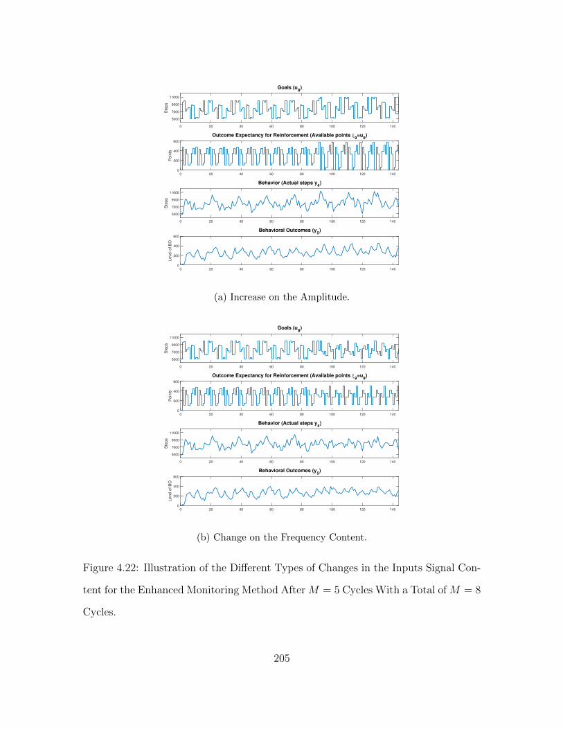
0 20 40 60 80 100 120 140

Ste

ps

5000

7000

9000

11000

Goals (u8)

0 20 40 60 80 100 120 140

Poin

ts0

200

400

600

Outcome Expectancy for Reinforcement (Available points 99=u

9)

0 20 40 60 80 100 120 140

Ste

ps

5000

7000

9000

11000

Behavior (Actual steps y4)

0 20 40 60 80 100 120 140

Level of B

O

0

200

400

600


(a) Increase on the Amplitude.

0 20 40 60 80 100 120 140

Ste

ps

5000

7000

9000

11000

Goals (u8)

0 20 40 60 80 100 120 140

Poin

ts

0

200

400

600


9)

0 20 40 60 80 100 120 140

Ste

ps

5000

7000

9000

11000

Behavior (Actual steps y4)

0 20 40 60 80 100 120 140

Level of B

O

0

200

400

600


(b) Change on the Frequency Content.

Figure 4.22: Illustration of the Different Types of Changes in the Inputs Signal Con-

tent for the Enhanced Monitoring Method After M = 5 Cycles With a Total of M = 8

Cycles.

205

realistic constraints. The first case represents an increase in the amplitude of the input

signals after M = 5 cycles. The maximum daily goal is incremented to 11000 steps

per day, the minimum number of available points is now 0 and the maximum number

of points is increased to 600 as is illustrated in Fig. 4.22a for a total of M = 8 cycles.

The second case represents a change on the harmonic related frequency content of

the inputs signals. For both inputs the consider harmonic reduction step after M = 5

cycles is from Sh,1 = 0 to Sh,2 = 1 for L = 2, as was defined in (4.64) – (4.66). A

simulation of the input-output signals for M = 8 cycles is shown in Fig. 4.22b.

Monitoring results are presented in Fig. 4.23 for the two mentioned cases and

the initial case with no modifications in the signals. The first plot represents the

maximum additive uncertainty ε(M) as is computed in (4.104). The second plot

presents computations of the approximate robust performance index and its respective

test according to (4.110) – (4.111), and the third plot presents again fits to a different

cross-validation data set.

The increment on amplitude represents the best improvement for identification

purposes. The maximum additive uncertainty is reduced and the robust performance

test is now accomplished after M = 8 cycles. Checking cross-validation results it can

be observed that percentage fits increase at higher rates and they reach the desired

values faster. If the stopping criterion from (4.107) is now considered with BAV = 2%,

BRV = 15%, and nMi = 2 the experiment can be halt after M = 11 cycles as is shown

in Table 4.5.

When modifications in the harmonic frequency content of the input signals are

implemented, improvements on identification results are also observed. Now the

robust performance test indicates that the experiment can stop after M = 9 cycles,

with better percentages of fit. Also the stopping criterion from (4.107) considering

BAV = 2%, BRV = 15%, and nMi = 2 indicates that the experiment can be halted

206

Number of cycles M

2 3 4 5 6 7 8 9 10 11 12 13 14 15 160

0.5

Additive uncertainty

~0(M) no changes

~0(M), amplitude change at M=5

~0(M), fund. freq. change at M=5

Number of cycles M

2 3 4 5 6 7 8 9 10 11 12 13 14 15 16

1

1.5

2Approximate robust stability test

gRPimax(M) no changesgRPimax(M), amplitude change at M=5gRPimax(M), fund. freq. change at M=5

Number of cycles M

2 3 4 5 6 7 8 9 10 11 12 13 14 15 1630

35

40

Cross-validation fit to y4

%fity4(M) no changes

%fity4(M) amplitude change at M=5

%fity4(M) fund. freq. change at M=5

Figure 4.23: Illustration of the Enhanced Identification Test Monitoring Method,

Testing all the Possible Actions Over the Input Signals After M = 5 Cycles: no

Changes, Increments on the Amplitude, and Changes on the Harmonic Related Fre-

quencies for M = 1, · · · , 16.

after M = 13 cycles as is detailed in Table 4.6. The stopping criterion based on

percentage uncertainty reductions is more conservative since it computes a MIMO

metric based on singular values, and it uses the maximum value over all the frequency

grid.

The performance of the process is tested now utilizing 10 replications of different

noise structures: The original Gaussian noise with σ24 = 300000, σ2

5 = 500 , and the

autoregressive structure of (4.142). Initially the pure autoregressive case is considered

207

Table 4.5: Percentages of Uncertainty Reduction According to (4.105) – (4.106) for

Increments on the Amplitude of the Input Signals.

M 3 4 5 6 7 8 9

AV (%) -23.39 44.97 14.27 6.32 17.5 2.85 5

RV (%) -23.39 36.44 18.2 9.85 30.26 7.07 13.34

M 10 11 12 13 14 15 16

AV (%) 0.16 1.39 1.52 1.11 1.71 1.36 0.9

RV (%) 0.5 4.31 4.92 3.76 6.03 5.1 3.55

Table 4.6: Percentages of Uncertainty Reduction According to (4.105) – (4.106) for

Changes on the Frequency Content of the Input Signals.

M 3 4 5 6 7 8 9

AV (%) -23.39 44.97 14.27 11.93 10.35 1.67 4.86

RV (%) -23.39 36.44 18.2 18.6 19.81 3.98 12.08

M 10 11 12 13 14 15 16

AV (%) 1.69 4.04 1.66 1.16 0.76 0.24 -0.25

RV (%) 4.79 11.99 5.59 4.15 2.84 0.93 -0.98

208

with σ24 = 300000 and φ = 0.7, then a more integral noise configuration with σ2

4 =

300000, and φ = 0.9 is applied. Results are shown in Fig. 4.24a and Fig. 4.24b. For

all cases the robust performance test is eventually accomplished after some iterations.

The percentage fits are more variable for the autoregressive and integral cases that

demand more power from the inputs.

With the obtained informative model utilizing M = 12 cycles, the optimized

experiment is implemented again with a fixed duration of 273 days. The obtained

inputs and the resultant simulated outputs are shown in Fig. 4.25. The same set of

cross-validation data is used and resulting fits are 42.41% for behavior and 64.65% for

outcome expectancy; validation plots for both informative and optimized experiments

are shown in Fig. 4.26.

Patient-friendlessness indexes from inputs-output data are again computed an

tabulated in Table 4.7 according to equations (4.137) – (4.140). Once again improve-

ments resulting from the optimized experiment can be observed in percentage fits and

in the reduced variability of input-output data.

4.6 Chapter Summary

In this chapter a system identification procedure has been described which includes

both experimental (input signal) design and grey-box (semi-physical) parameter es-

timation for a physical activity intervention described by a dynamical systems model

for Social Cognitive Theory (SCT). Input signal design is performed in two stages:

one called the informative where signals are designed using either a randomized tech-

nique or an identification test monitoring process, and an optimized experiment where

signals are designed to improve the response of the intervention from a behavioral

standpoint, and to obtain an acceptable model for the system.

In the informative stage different input signal design strategies were presented.

209

Number of cycles

2 3 4 5 6 7 8 9 10 11 12 13 14 15 160

2

4

6

8

10


Test bound

Number of cycles

2 3 4 5 6 7 8 9 10 11 12 13 14 15 1630

35

40

45

50

10 realizations of %fity4(M )

(a) Gaussian Noise.

Number of cycles

2 4 6 8 10 12 14 16 18 20 22 24 26 28 30 32 34 36 38 400

2

4

6

8

10

12

14



Test bound

Number of cycles

2 4 6 8 10 12 14 16 18 20 22 24 26 28 30 32 34 36 38 4028

30

32

34

36

38

40

42

44

46

10 realizations of %fity4(M)

Number of cycles

2 4 6 8 10 12 14 16 18 20 22 24 26 28 30 32 34 36 38 400

5

10

15

20

25INTEGRAL NOISE


Test bound

Number of cycles

2 4 6 8 10 12 14 16 18 20 22 24 26 28 30 32 34 36 38 4028

30

32

34

36

38

40

42

44

10 realizations of %fity4(M)

(b) Autoregressive and Integral Noise.

Figure 4.24: Ten Replications of the Enhanced Monitoring Process for Different Noise

Structures, Including Gaussian With σ24 = 300000, σ2

5 = 500, Autoregressive With

σ24 = 300000 and φ = 0.7, and Integral With σ2

4 = 300000, and φ = 0.9.

210

0 50 100 150 200 2500

2000

4000

6000

8000

10000

12000

Time (days)

Ste

ps

Goals (ξ8=u

8)


)

Behavior (ysim

=η4

sim)

0 50 100 150 200 2505

10

x 104

Ste

ps

External cues (Goals ξ8=u

8)

0 50 100 150 200 2500

200

400

Poin

ts


9)

0 50 100 150 200 2500

200

400

Poin

ts


=u10

)

Figure 4.25: Input/output Data for the Optimized Experiment Derived From the

Enhanced Monitoring Process.


tive and Optimized Experiments Resulting From the Enhanced Monitoring Process.


∆u8 (steps) 1684.6 958.72

S∆u8 (steps) 1534.7 934.57

∆u9 (points) 184.84 54.526

S∆u9 (points) 104.85 124.16

esim (steps) 4810.6 3681.8

Sesim (steps) 4748.4 3787

211

0 10 20 30 40 50 60 70 80 902000

4000

6000

8000

10000

12000

Time(days)

Ste

ps

Behavior (y4)

0 10 20 30 40 50 60 70 80 90-100

0

100

200

300

400

500

Time(days)

leve

l o

f B

O


Simulation plant

Informative model

Optimized model

%fit4(Inf.) = 40.06%

%fit5(Inf.) = 51.74%

%fit4(Opt.) = 42.41%

%fit4(Opt.) = 64.65%


Identified Model From the Informative and Optimized Experiments Resulting From

the Enhanced Monitoring Process.

First a fixed time randomized generation of input signals subject to operational am-

plitude constraints. As a second alternative, a monitoring approach is designed to

find the shortest possible experiment that is “good enough” for identification pur-

poses; this was done through the computation of asymptotic statistical uncertainties

that are accurate for a large number of periods M , and conservative otherwise. Ini-

tially a basic monitoring procedure was proposed where an evaluation of the signal

quality is performed every period yielding to the decision to halt the experiment or

to aggregate an additional period of the same signal. This transfer function based

estimation procedure enabled the specification of input-output directions of interest

for the identification problem. Finally and enhanced monitoring method is presented

which incorporates the possibility to perform changes in the amplitude or in the har-

212

monic frequency content of the input signals. The proposed experimental stopping

criterion relies on robust performance ideas. For the optimized experiment it was

shown that the design of the required inputs within practical operating limitations

can be formulated as a feasible constrained optimization problem.

Independent simulation studies are presented for each input signal design ap-

proach. For the fixed time case, an acceptable percentage of fit can be observed,

even in the presence of external disturbances. In the informative experiment a set of

data exhibiting high variability is obtained (Fig. 4.8); in the optimized experiment

the variability in the data is reduced (Fig. 4.10) while obtaining a model that dis-

plays a higher level of predictive ability. It is important to highlight the fact that the

input/output signals from the optimized experiment showed a better performance in

terms of “patient-friendliness” and desired behavior tracking, as could be observed in

Table 4.2. The resultant behavior from the optimized experiment strongly depends

on the initial results from the informative stage. If the informative estimation results

are biased then the optimized output is also expected to be biased, however if the

informative experiment succeeds in predicting the variability of the system, a pattern

similar to the desired one is expected in the optimized output.

For the basic monitoring process input magnitudes were held constant while the

length of the experiment was under periodic evaluation. The simulation study con-

sidered the simultaneous effect of noise in all the measured outputs and the presence

of disturbance inputs, to resemble a more realistic situation. Simulation results il-

lustrated how by applying the monitoring process, a shorter informative experiment

could be defined that still captures the dynamics of the system. Acceptable fits could

be obtained (Fig. 4.18) and again good signals in terms of “patient-friendliness” were

derived in the optimized stage as is observed in Table 4.4.

Finally the enhanced monitoring process is simulated considering two possible

213

additional modifications in the input signal content after each periodic evaluation:

increments in the amplitude, and changes in the harmonic related frequency content.

The proposed stopping criterion incorporates robust performance ideas; however if

one of the specified modifications on the input signal content is applied, then a more

general criterion based on percentage change of MIMO additive uncertainties can

be used. Fig. 4.27 shows a comparison between the basic and the enhanced MIMO

uncertainty computation index ε(M) using (4.56) and (4.104), considering the same

“zippered” input signal. As expected the enhanced method provides a more con-

servative measurement of uncertainties; both methods present similar uncertainty

reduction tendencies when the length of the experiment is increasing. One advan-

tage of the enhanced method is that it does not require to wait until the signal has

reached its steady state; hence the evaluation can be started earlier. The use of the

enhanced method also enables the possibility of on-the-go modifications in the input

signal content.

214

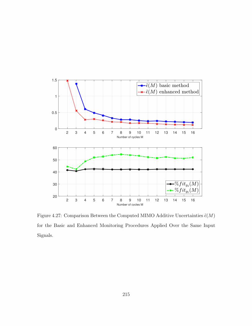
Number of cycles M

2 3 4 5 6 7 8 9 10 11 12 13 14 15 160

0.5

1

1.5

~0(M ) basic method~0(M ) enhanced method

Number of cycles M

2 3 4 5 6 7 8 9 10 11 12 13 14 15 1620

30

40

50

60

%fity4(M )%fity5(M )

Figure 4.27: Comparison Between the Computed MIMO Additive Uncertainties ε(M)

for the Basic and Enhanced Monitoring Procedures Applied Over the Same Input

Signals.

215

Chapter 5

DESIGN OF CLOSED-LOOP BEHAVIORAL INTERVENTIONS USING

HYBRID MODEL PREDICTIVE CONTROL

5.1 Overview

A variety of serious health conditions, among them breast and colon cancer, obe-

sity, diabetes, and cardiovascular disease, are linked to physical inactivity (McGin-

nis et al., 2002). For breast cancer in particular, estimates suggest that the risk

of developing this disease can be reduced by 20-30% by engaging in 30-60 minutes

of moderate-intensity physical activity (PA) per day (Clague and Bernstein, 2012).

However, most researcher-developed mHealth PA interventions have only been evalu-

ated in short-term pilots (e.g., 4 weeks to 6 months) with modest effects (Payne et al.,

2015) and require an assessment of their effectiveness under real-world conditions that

include maintenance. There is a need for interventions that can cost-effectively scale,

adapt to each person’s changing needs, and provide support as long as needed. Most

evidence-based PA interventions are delivered by a person, thus limiting scalability,

data-driven adaptability, and long-term use (Marcus et al., 2006). Almost all inter-

ventions, including digital ones, are designed for fixed durations, which is problematic

when circumstances, health conditions, or goals change. Previous evidence supports

the notion that PA is a highly variable behavior, with the general trend of individuals

moving towards less PA (Rauner et al., 2015). There is a need for interventions that

provide treatment when necessary, quietly monitor when not needed, and re-emerge

when a relapse is imminent.

In previous chapters a dynamical model for Social Cognitive Theory (SCT) (Ban-

216

dura, 1986) was developed using fluid analogies to represent the different constructs

of the theory and their interactions. Using an open-loop PA intervention as a refer-

ence, a set of system identification experiments at an idiographic (i.e., single subject)

level have been designed to search and refine the model parameters and for validation

purposes. Relying on these ideas a pilot mHealth intervention called “Just Walk” is

currently being tested (Hekler, 2015), this intervention provides daily “ambitious but

doable” step goals and reinforcements (i.e., points) for achieving goals.

In this chapter, the purpose is to develop a decision algorithm for a closed-loop

mHealth Intensively Adaptive Intervention (IAI; Riley et al. (2015b)) to promote PA

(measured in terms of daily steps) among sedentary adults. To achieve successful

outcomes of the intervention in the long term, two phases are included: a behavioral

initiation training stage where individuals are progressively driven to a healthy status

through the introduction of daily step goals and rewards, and a maintenance train-

ing phase where rewards are gradually decreased based on the enhanced capacity of

individuals to continuing engaging in the required behavior. The decision framework

for the intervention relies on a Hybrid Model Predictive Control (HMPC) formula-

tion (Nandola and Rivera, 2013); in general model predictive controllers have proved

their effectiveness on multivariable problems with operational constraints in diverse

application areas. HMPC-based solutions have recently been considered in behavioral

health settings (Deshpande et al., 2014a; Dong et al., 2013; Timms et al., 2014d). As

the basis for decision policies, they enable optimization of intervention dosages in the

presence of interaction between continuous and discrete signals that are commonplace

in behavioral interventions.

The HMPC-based decision policy presented here relies on a mixed logical dynami-

cal (MLD) framework to describe discrete sets of goals and rewards as the intervention

components. It is also used to represent the logical process of awarding rewards only

217

if daily goals are achieved. The formulation employs a three degree-of-freedom modal-

ity to independently adjust the speeds of set-point tracking, measured disturbance

rejection and unmeasured disturbance rejection. Controller reconfiguration through

the manipulation of penalty weights is proposed to address the transition between

the initiation and maintenance phases. Simulation results showing a hypothetical

scenario for a PA intervention are presented to illustrate the benefits of the proposed

approach in addressing the hybrid nature of the system, set point tracking, distur-

bance rejection, and the transition between the two stages of the intervention.

This chapter is organized as follows. Section 5.2 describes the different components

and conditions of the intervention. Section 5.3 presents details about the formula-

tion of the HMPC based adaptive intervention, including the discrete and logical

constraints and the controller reconfiguration to support the maintenance stage. Sec-

tion 5.4 presents a simulation study to test the performance of the controller under

conditions of disturbances. Section 5.5 gives a summary and conclusions of the chap-

ter.

5.2 Adaptive Closed-Loop Behavioral Intervention Based on SCT

The main purpose of the proposed intervention is to promote physical activity

among sedentary individuals, with the specific goal of achieving 10,000 steps per day

(or +3,000 steps/day more than baseline) on a weekly average. The goal will be

reached via the design and implementation of an effective intervention for behavior

change that is theoretically grounded on Social Cognitive Theory (SCT) (Bandura,

1986). In Chapter 4 a dynamical model of SCT for the low physical activity prob-

lem was developed relying on a fluid analogy that depicts the constructs and their

interrelationships described by the theory. As in the open-loop case, the closed-loop

intervention relies on the simplified version of the SCT model representing a “be-

218

haviorist” articulation of the determinants of behavior (Ferster, 1970), depicted in

Fig. 4.1. Assuming first order dynamics, the model is described by the set of differ-

ential equations (4.1) – (4.5).

The proposed closed-loop behavioral adaptive intervention is depicted in Fig. 5.1,

where the amount of performed daily steps is measured by the signal y4. It relies on

the systematic delivery of the following components, based on the actual performance

of individuals:

• Daily goals u8, to establish in a quantitative form the desired behavior (e.g.,

10, 000 steps per day).

• Expected points u9, the announced daily reward points that will be granted to

individuals if they achieve the daily goal.

• Granted points u10, given every day if individuals reach the set goal; this fea-

ture is represented by the “If/Then” block. Points can later be exchanged for

tangible rewards (e.g., gift cards).

η4

ξ4

ξ9

ξ10

Simplified

SCT

Model

ξ7

Goals

Decisionalgorithm


Desireddaily steps

u8

Expected points

If / Then

Grantedpoints

u9

u10 Behavioral outcomes

Behavior (steps)

η5

y4+

_

ξ11

Goalattainment

u11

Self-efficacyη3

Outcome expectancy

η2

Steps self-regulatorvia internal cues

+

_

csr

Figure 5.1: Conceptual Representation of the Closed-Loop Behavioral Adaptive In-

tervention, Based on the Simplified Version of the SCT Model in Fig. 4.1

219

The intervention is implemented using an SCT model enhanced with individual-

ized self-regulation via internalized cues as was described in Section 4.2.2. Relying

on the internal model control approach (IMC; Morari and Zafiriou (1989)) the self-

regulator is represented in a classical feedback controller form as

csr =qsr

1− p44qsr=

Ksr

β46γ64

· τ4s+ 1

λs+ 1−Ksr

(5.1)

where β46, γ64, and τ4 are part of the SCT model parameters, the transfer function

p44 represents the effect from input ξ4 to output η4, and qsr is the self-regulator

expressed in q-parametrization form. The performance of the system is characterized

by the value of the parameter λ that reflects the closed-loop speed of response and the

parameter Ksr that ranges from 0 to 1, with 1 representing perfect integral action.

The signal goal attainment (u11) is computed as the difference between the daily

goal and the actual performed behavior, affecting self-efficacy. This signal is used

to represent the ideal step-goal range feature presented in Section 2.7.2, where in-

dividuals might react negatively to too high a goal that they consider difficult to

reach.

5.3 Formulation of the HMPC-Based Adaptive Intervention

The purpose of the adaptive intervention is to have individuals achieve a desired

level of daily steps, while considering some important physical and operational con-

straints such as:

• Maximum and minimum values for goals and points (u8, u9 and u10) depending

on physical conditions (e.g., maximum and minimum daily step goals for an

individual). Financial limitations lead to bounds on the expected reward points,

since these have a direct conversion into monetary value.

• Goals and reward points must be drawn from discrete sets of integer values that

220

may represent meaningful effects on the intervention. As prior physical activity

experiments have pointed (King et al., 2013; Adams et al., 2013) having a fixed

set of goals and points could be important to analyze specific aspects of interest

on the intervention.

• The intervention may be configured in different stages where some of the inputs

may be deactivated or partially activated. For instance, when the behavior has

reached the desired level and is successfully sustained, a gradual decrease on

rewards may be activated.

The ensuing subsections describe the detailed formulation of the HMPC-based deci-

sion policy.

5.3.1 Use of the HMPC framework

The control strategy for intervention design must incorporate the defined re-

quirements and constraints for the physical activity behavioral intervention. A Hy-

brid Model Predictive Control strategy (HMPC; Nandola and Rivera (2013)) will

be further studied and applied to this problem since it incorporates hybrid dynam-

ics through mixed logical dynamical (MLD) representations (Bemporad and Morari,

1999); this feature can be used to represent the natural constraints of the problem.

Hybrid dynamical systems consider discrete and continuous events simultaneously;

they can be represented by differential (or difference) equations and logical condi-

tions describing their categorical or binary response. The aim of the control design

will be directed to the following tasks:

• Setpoint tracking: Goals and expected reward points are assigned to obtain

the desired amount of daily steps following continuous and discrete constraints.

221

• Measured disturbance rejection: The controller manipulates goals and ex-

pected points to mitigate the effect from measured external disturbances (e.g.,

environmental context) using the subsection of the identified SCT model that

is related to those signals. For instance if some environmental event (e.g., bad

weather) is known a priori, then goals or rewards can be adjusted to compensate

for that disturbance.

• Unmeasured disturbance rejection: Inputs are manipulated to mitigate

the effect of unknown and possibly unmodeled external influences. For example,

any unexpected situation that may impact the disposition of the individual for

physical activity (e.g., sickness of a family member, sudden party invitation)

can be mitigated by adjustments on goals or points by the controller.

Model predictive control (MPC; Camacho and Bordons (2004)) is a controller

formulation where the current values of the manipulated variables (i.e., inputs) are

determined in real time as the solution of an optimal control problem over a horizon

of given length. The optimization problem is solved for a move horizon using a model

(e.g., the identified SCT model) from where a new set of control moves are obtained;

outputs from the system are then computed over the prediction horizon with the

current plant state estimate (i.e., output measurement) assumed as the initial state.

Only the first calculated moves are applied at each instant; the whole process is then

repeated and new control moves are obtained. This receding horizon control strategy

is depicted in Fig. 5.2 considering set goals (u8) as the manipulated variable, actual

steps (y4) as the controlled variable, and environmental context (d7) as measured

disturbance.

The HMPC controller relies on the MLD structure that describes a hybrid linear

system including real and integer states, inputs and constraints, and is represented

222

Prediction Horizon

Forecasted Environmental Context Report d(k+i) (if available)

Predictedsteps f

Prior steps Report (Measured Outcome)

Future Step Goals a

Prior Environmental Context Report

(Measured Disturbance)

Prior Step Goals

k k+1 k+m k+p

Move Horizon

Desired steps (Setpoint rr )

Dis

turb

.

Vari

ab

le

Co

ntr

olled

Vari

ab

le

Man

ipu

late

d

Vari

ab

le

Past Future

Time (days)

y4(k + i)

d7(k + i)

u8(k + i)umax

8

umin8

y4r(k + i)

Figure 5.2: Conceptual Application of the Receding Horizon Control Strategy to

the Physical Activity Behavioral Problem Considering Step Goals (u8) as the In-

put, Actual Steps (y4) as the Output, and Environmental Context (d7) as Measured

Disturbance.

as

x(k + 1) = Ax(k) +B1u(k) +B2δ(k) +B3z(k) +Bdd(k) (5.2)

y(k + 1) = Cx(k + 1) + d′(k + 1) + v(k + 1) (5.3)

E2δ(k) ≤ E5 + E4y(k) + E1u(k)− E3z(k)− Edd(k) (5.4)

where in general x = [xTc xTd ]T , xc ∈ Rncx , xd ∈ {0, 1}ndx , and u = [uTc uTd ]T , uc ∈

Rncu , ud ∈ {0, 1}ndu are systems states and inputs with continuous and discrete ele-

ments; y ∈ Rny is the vector of outputs; d, d′, and v are measured disturbances,

223

unmeasured disturbances, and measurement noise respectively. δ ∈ {0, 1}nδ and

z ∈ Rnz are discrete and continuous auxiliary variables that are introduced in order

to convert logical and discrete decisions into their equivalent linear inequality con-

straints represented in (5.4). Variables nx = ncx + ndx, nu = ncu + ndu, ndist, and ny are

the total number of states, inputs, measured disturbances, and outputs, respectively.

Dimensions of auxiliary variables and the number of linear constraints in (5.4) depend

on the specific character of the discrete and logical decisions in the particular hybrid

system.

A standard quadratic cost function is used to calculate the decision vector for the

optimization problem as

J ,p∑i=1

‖y(k + i)− yr‖2Qy +

m−1∑i=0

‖∆u(k + i)‖2Q∆u

+m−1∑i=0

‖u(k + i)− ur‖2Qu

+

p−1∑i=0

‖δ(k + i)− δr‖2Qδ

+

p−1∑i=0

‖z(k + i)− zr‖2Qz

(5.5)

where p is the prediction horizon, m is the control (or move) horizon. The matrices

Qy, Q∆u, Qu, Qδ, and Qz are the penalty weights on the error, move size, control

signal, auxiliary binary variables, and auxiliary continuous variables respectively. The

weighted norm of a vector r = [r1 · · · rn]T can be defined as:

‖r‖2Qr = rT ·Qr · r (5.6)

with Qr =

wr1 0 · · · 0

0 wr2 · · · 0

......

. . ....

0 0 · · · wrn

(5.7)

where each wri is the correspondent weight or relative importance of the element ri.

The problem is formulated as a tracking control system where yr, ur, δr, and zr are the

references for output, input, discrete and continuous auxiliary variables respectively.

224

The optimization problem consists of finding the sequences of control actions u(k)

,.., u(k +m− 1), δ(k) ,.., δ(k + p− 1), and z(k) ,.., z(k + p− 1) that minimize J as

min{[u(k+i)]m−1

i=0 ,[δ(k+i)]p−1i=0 ,[z(k+i)]p−1

i=0 }J (5.8)

subject to the mixed integer constraints described in (5.4) and the following various

process constraints:

ymin ≤ y(k + i) ≤ ymax, 1 ≤ i ≤ p (5.9)

umin ≤ u(k + i) ≤ umax, 0 ≤ i ≤ m− 1 (5.10)

∆umin ≤ ∆u(k + i) ≤ ∆umax, 0 ≤ i ≤ m− 1 (5.11)

Unmeasured disturbances d′ are described as general non-stationary stochastic

signals by

xw(k) =Awxw(k − 1) +Bww(k − 1) (5.12)

d′(k) =Cwxw(k) (5.13)

where w(k) is a vector of integrated white noise. In this formulation single integrating

disturbances are assumed, hence Bw = Cw = I and Aw = 0ny×ny are assumed. These

results yields to an augmented representation of the system as

X(k) =AX(k − 1) + B1∆u(k − 1) + B2∆δ(k − 1) + B3∆z(k − 1)

+ Bd∆d(k − 1) + Bw∆w(k − 1)

(5.14)

y(k) = CX(k) + ν(k) (5.15)

where

X(k) =

(∆xT (k) ∆xTw(k) yT (k)

)T(5.16)

A =

A 0 0

0 Aw 0

CA Aw I

(5.17)

225

Bi =

Bi

0

CBi

, i = 1, 2, 3, d; Bw =

0

I

I

; C =

(0 0 I

)(5.18)

These equations are used to build a filtered observation X(k/k) and a prediction

Y(k + 1) for p steps into the future where

Y(k + 1) =

(yT (k + 1) yT (k + 2) · · · yT (k + p)

)T(5.19)

A detailed explanation about the formulation of the algorithm including the definition

of all the scalar and vectorial coefficients is presented in (Nandola and Rivera, 2013).

The HMPC formulation relies on a three degree-of-freedom tuning process, where

setpoint tracking, measured and unmeasured disturbance rejections can be adjusted

independently by varying parameters αjr, αld and f ja from 0 to 1, for j = 1, · · · , ny,

and l = 1, · · · , ndist. This process is depicted in Fig. 5.3, where P and Pd are the

multivariable plant and disturbance models, respectively. For setpoint tracking the

filter matrix F (q, αr) is

F (q, αr) =

f(q, α1r) 0 · · · 0

0 f(q, α2r) · · · 0

......

. . ....

0 0 · · · f(q, αnyr )

(5.20)

where each f(q, αjr) is a Type-I discrete-time filter (Morari and Zafiriou, 1989) defined

as

f(q, αjr) =(1− αjr)qq − αjr

, j = 1, · · · , ny (5.21)

The speed of setpoint tracking can be adjusted by manipulating coefficients αjr from

0 to 1. The smaller the value for αjr, the faster the output response for setpoint

tracking.

226

P

PddiF (q,!r)

F (q,!d)

+ + +

+

unu!1

yrny!1

yny!1

dndist!1

d!ny"1

vny!1

+

++min!

JY(k + 1)

X(k/k), Kf

Figure 5.3: Block Diagram Depicting the Three Degree-of-Freedom Tuning Within

the HMPC Formulation. P and Pd Are the System Plant Models, X(k/k), Kf is the

Observer Block, Y(k + 1) is the Predictor Block, F (q, αx), x = r, d are the Filters for

Reference and Measured Disturbance Signals, and the Block Referred as “min J” is

the Optimizer Where ρ is the Vector of Decision Variables.

For measured disturbance rejection the formulation relies on an externally gener-

ated forecast that is processed through the filter F (q, αd). In this work Type-I filters

are considered

F (q, αd) =

f(q, α1d) 0 · · · 0

0 f(q, α2d) · · · 0

......

. . ....

0 0 · · · f(q, αndistd )

(5.22)

f(q, αld) =(1− αld)qq − αld

, l = 1, · · · , ndist (5.23)

however a Type-II filter structure should be used if the integrating system dynamics

are present (Nandola and Rivera, 2013). Coefficients αld are used to adjust the speed

of measured disturbance rejection. These parameters must have values lying between

0 and 1; the lower the value of each αld, the faster the speed of disturbance rejection.

227

The optimizer uses the model and current measurements y(k) to compute future

states through an observer/filter. To achieve the full three degree-of-freedom feature

it is necessary to decouple the effects of measured and unmeasured disturbance, hence

the augmented state estimator is computed as

Xflt(k|k) = Xflt(k|k − 1) +Kf

(y(k)− CX(k|k − 1)

)(5.24)

where Xflt is computed considering the filtered measured disturbance, whileX utilizes

the unfiltered measured disturbance such that the second term in (5.24) represents

the effect of unmeasured disturbance only. The term

PE = y(k)− CX(k|k − 1) (5.25)

is the prediction error. The process is described with details by Nandola and Rivera

(2013).

The observer weights the effect of the unmeasured disturbances through the gain

matrix Kf . The optimal value of Kf is computed using the parametrization shown in

Lee et al. (1994) and Lee and Yu (1994) that enables the independent specification of

unmeasured disturbance rejection for each output channel. The closed-loop response

of the system is affected by the tuning method, creating a direct link with robust

stability and robust performance ideas (Morari and Zafiriou, 1989). Kf is defined as

Kf = [0 F Tb F T

a ]T (5.26)

where

Fa =

f 1a 0 · · · 0

0 f 2a · · · 0

......

. . ....

0 0 · · · fnya

(5.27)

228

Fb =

(f 1a )2 0 · · · 0

0 (f 2a )2 · · · 0

......

. . ....

0 0 · · · (fnya )2

(5.28)

Equation (5.28) is formulated under the assumption of white noise. Each f ja ,

j = 1, · · · , ny is a tuning parameter that lies between 0 and 1, affecting how the

controller reacts to unmeasured disturbances that are present at each output. If one

of these coefficients approaches 0, then for that particular output the controller ignores

the prediction error correction, and decisions are done mainly based in the model and

the controller structure. If parameters f ja are close to 1, the controller relies more

on prediction errors, which are affected by unmeasured disturbance and unmodeled

dynamics, and its action over the inputs can become very aggressive. The clear effect

of Fa on the sensitivity and complementary sensitivity functions is discussed in Lee

and Yu (1994).

For the closed-loop physical activity intervention the considered input and output

vectors are

u = [u8 u9 u10]T , nu = 3 (5.29)

y = [y2 y3 y4 y5]T , ny = 4 (5.30)

Environmental context is considered as the measured disturbance d = ξ7, the unmea-

sured disturbance is assumed Gaussian and affecting only performed daily steps (i.e.,

output y4 = η4).

5.3.2 Discrete and Logical Constraints

Discrete and logical features of the physical activity behavioral intervention can

be described using the MLD framework. Intervention components take their val-

229

ues from discrete sets of events, the possible set of step goals is defined as u8(k) ∈

U8 = {Cv1, · · · , Cvnu8}, and the possible set of available points is u9(k) ∈ U9 =

{Cvnu8+1, · · · , Cvnu8+nu9}, hence the following logical and continuous auxiliary vari-

ables are defined as

δj(k) = 1⇔ zj(k) = Cvj, j = 1, · · · , nu8 + nu9 (5.31)

This condition is enforced by

zj(k) = Cvjδj(k), j = 1, · · · , nu8 + nu9 (5.32)

To assure that only one value can be assigned to u8 and u9 at each sampling time it

is necessary to add the following constraints:

nu8∑j=1

δj(k) = 1, u8(k) =

nu8∑j=1

zj(k) (5.33)

nu8+nu9∑j=nu8+1

δj(k) = 1, u9(k) =

nu8+nu9∑j=nu8+1

zj(k) (5.34)

The effect of all the inputs at any given day will be reflected on the outputs at the

following day, hence the number of performed steps y4(k) is resultant from the goals

and points from the previous day u8(k − 1), u9(k − 1), and u10(k − 1). According

to the proposed intervention depicted in Fig. 5.1, the “If/Then” block is responsible

for determining if the points are granted, depending on the fulfillment of daily goals.

The auxiliary logical variable δ10 is set as true when the performed steps are greater

or equal than the goal set the previous day

δ10(k) = 1⇔ y4(k) ≥ u8(k − 1) (5.35)

A big-M reformulation is applied to convert logical constraints to a set of linear

conditions with the same feasible set. To assign the corresponding value of δ10 the

230

following constraints are considered:

y4(k)− u8(k − 1) ≤ δ10(k)[ymax4 − umin8 ] (5.36)

y4(k)− u8(k − 1) ≥ [1− δ10(k)][ymin4 − umax8 ] (5.37)

The auxiliary variable z10 is used to represent the granted points, hence

u10(k) = z10(k) (5.38)

At the beginning of every day, goal attainment is verified; if the goals have been met,

the points announced the previous day are granted (u10 = u9). This is imposed by

u9(k − 1)− z10(k) ≤ [1− δ10(k)][umax9 − umin10 ] (5.39)

u9(k − 1)− z10(k) ≥ [1− δ10(k)][umin9 − umax10 ] (5.40)

If the goals are not achieved, no points are given that day (u10 = 0)

z10(k) ≥ δ10(k)umin10 (5.41)

z10(k) ≤ δ10(k)umax10 (5.42)

The constraints described by (5.31) - (5.42) are incorporated to the system presented

in (5.4) by defining the values for matrices E1, E2, E3, E4, E5, and Ed. This is per-

formed using the Hybrid Systems Description Language (HYSDEL; Torrisi and Be-

mporad (2004)), which is a software tool that helps to the construction of the MLD

representation matrices, using a high level description of the logical inputs, states,

outputs, and other logical rules.

5.3.3 Maintenance Training Stage

Once the desired goal has been reached and sustained for a predetermined num-

ber of days, a maintenance training stage of the intervention is initiated. Here the

231

HMPC algorithm must be reconfigured so as to maintain the daily performed steps

in spite of a reduction of the number of points, and, if needed, reactivating the use of

points if a significant relapse occurs. To adapt the HMPC performance to these new

considerations, the penalty weights in the objective function are adjusted during the

course of the intervention.

During the initiation phase, the main goal is to achieve the required daily steps.

The reference output set point is yr = [yr2 yr3 yr4 yr5]T , where yr4 is the desired

amount of daily steps (e.g., 10000). Considering vectors u and y defined in (5.29)

– (5.30) the following weight matrices Qu and Qy are considered in the objective

function (5.5) to impose a set point tracking only on the variable y4 (daily steps)

Qu =

0 0 0

0 0 0

0 0 0

, Qy =

0 0 0 0

0 0 0 0

0 0 1 0

0 0 0 0

(5.43)

The remaining weight matrices in (5.5) are considered zero-valued.

The maintenance stage is enabled when the goal has been achieved and sustained

at least nm − 2 times during the last nm days. The goal is considered achieved

when the difference between the actual steps and the reference is within a predefined

tolerance tol4. A new auxiliary logical variable δgoal(k), that is not included in the

general HMPC formulation per (5.2)-(5.4), is defined as

δgoal(k − i) = 1⇔ |y4(k − i)− yr4 | ≤ tol4

i = 0, · · · , nm − 1

(5.44)

hence the second phase is activated at the sample time k if

nm−1∑i=0

δgoal(k − i) ≥ nm − 2 (5.45)

232

During this phase it is necessary to reconfigure the controller to target a low use of

points (u9). If the target inputs are: ur = [ur8 ur9 ur10 ]T , an appropriate value for

ur9 must be selected (e.g., ur9 = 0 points) and the weight matrix Qu is changed to

Qu =

0 0 0

0 wu9 0

0 0 0

(5.46)

The value of wu9 depends on the expected performance of the set point tracking versus

the input targeting. The matrix Qy remains as was defined in (5.43) and the rest of

the weight matrices are zero-valued. If at any time k the condition specified in (5.45)

is not accomplished (e.g., a relapse), the initiation phase is reactivated.


The simulation results presented in this section assume a hypothetical individual

with a sedentary lifestyle, performing an average (i.e., baseline) of 5000 steps per day

with an intervention starting at day zero. This simulation scenario is considered to

resemble the performance observed on previous physical activity interventions with

similar components (King et al., 2013). The assumed model parameters are

• τ2 = 40, τ3 = 30, τ4 = 0.8, τ5 = 2, τ6 = 0.5

• γ311 = 0.4, γ29 = 2.5, γ57 = 1, γ510 = 0.6, γ64 = 1.5

• β25 = 0.5, β34 = 0.2, β42 = 0.3, β43 = 0.9, β45 = 0.5, β46 = 0.9, β54 = 0.6

Delays (θi) and internal disturbance parameters (ζi) are considered zero. The self-

regulator via internalized cues described in (4.12) is considered with Ksr = 0.8 and

λ = 1. Parameters for the HMPC are as follows: the sampling time is Ts = 1 day, the

controller horizons are p = 7 and m = 5 days, maximum and minimum bounds are

umin =[5000 0 0]T

233

umax =[10000 500 500]T

∆umin =[−1000 − 500 − 500]T

∆umax =[1000 500 500]T

ymin =[0 0 0 0]T

ymax =[10000 10000 12000 10000]T

The weight matrices are defined as is shown in (5.43) including the reconfigured matrix

Qu described in (5.46) with wu9 = 0.005. The categorical values of the intervention

components are defined by the sets

U8 ={5000, 6000, 7000, 8000, 9000, 10000}

U9 ={100, 200, 300, 400, 500}

with nu8 = 6 and nu9 = 5. The unmeasured disturbance is assumed Gaussian with

d′(k) ∼ N (0, 40000).

Considering the input/output definitions for this problem, the vectors representing

the different tuning parameters according to (5.20), (5.22), and (5.27) are expressed

as

αr = [α2r α3

r α4r α5

r ]T (5.47)

αd = α4d (5.48)

fa = [f 2a f 3

a f 4a f 5

a ]T (5.49)

To allow for a progressive increase on the performed steps and a fast disturbance

rejection the considered tuning parameters are αr = [0 0 0.96 0]T , αd = 0.1,

fa = [0 0 0.3 0]T .

Initial simulation results are shown in Fig. 5.4 where no plant-model mismatch is

assumed. Goals (u8) and available points (u9) are generated by the HMPC algorithm.

234

Time (days)

0 10 20 30 40 50 60 70 80 90 100 110 120 130 140 150

Ste

ps

0

2000

4000

6000

8000

10000

Maintenance phase

Step goals (u8)


)

Daily steps (y4=2

4)

Goals (u8)

0 10 20 30 40 50 60 70 80 90 100 110 120 130 140 150

Ste

ps

5000

10000


9)

0 10 20 30 40 50 60 70 80 90 100 110 120 130 140 150P

oin

ts

0200400

0 10 20 30 40 50 60 70 80 90 100 110 120 130 140 150

Po

ints

0200400

Reinforcement (Granted Points 910

=u10

)

0 10 20 30 40 50 60 70 80 90 100 110 120 130 140 150

205080

Measured disturbance (Environmental context (d=97)

Figure 5.4: Simulation Results for the HMPC Based Adaptive Intervention for a

Participant With low Physical Activity, Considering d′(K) ∼ N (0, 40000), wu9 =

0.005, αr = [0 0 .96 0]T , αd = 0.1, and fa = [0 0 0.3 0]T .

It is observed that the value for granted points (u10) is taken from the available points

only when the previous day goal is achieved, as was enforced by the MLD constraints.

The maintenance stage of the intervention is illustrated via a shaded region; this phase

starts when the goal has been achieved for at least 4 times during the last nm = 6 days

with a tolerance of tol4 = 700 steps. During this stage a reduction in the amount of

available and granted points can be observed. The impact of measured disturbances

(e.g., environmental context) is tested via a downward pulse starting at the day 110,

and lasting for 15 days, as a result participants tend to reduce their steps and the

controller reacts by deactivating the maintenance phase and hence using the points

back to compensate any deviation.

235

0 50 100 150

Ste

ps

5000

6000

7000

8000

9000

10000

11000

Goals (u8)

0 50 100 150

Poin

ts

0

200

400

600

Available points (u9)

0 50 100 150

Poin

ts

0

200

400

600

Granted Points (u10

)

0 50 100 150

Dis

turb

an

ce

s

-50

0

50

100

Measured (env. context)

Unmeasured

Time (days)

0 50 100 150

Inte

rna

l c

ue

s (9

4)

100

200

300

400

500

600

700

800

Time (days)

0 50 100 150

Da

ily

ste

ps

(y

4)

2000

4000

6000

8000

10000

Desired behavior

Time (days)

0 50 100 150

Se

lf-e

ffic

ac

y (2

3)

-50

0

50

100

HMPC based intervention

Internalized cues only

Figure 5.5: Performance of the HMPC Physical Activity Intervention Versus a Self-

Regulation via Internalized Cues Case With a Pre-Defined Set of Incremental Step

Goals.

Fig. 5.5 shows a comparison between the performance of the HMPC intervention

against a second scenario where a set of incremental goals is the only defined input. In

this scenario individuals try to attain their goals through the internal self-regulation

via internalized cues process. The HMPC intervention displays a better tracking

to the final desired behavior of 10, 000 steps; this is achieved through an increase

of the individual’s self-efficacy via the offered and granted rewards. In the HMPC

case the higher self-efficacy lets the individual require less internal cues compared

to the internalized cues-only case, and allows the use of fewer points during the

236

maintenance phase. In both scenarios the self-regulation block tries to compensate

differences and/or disturbances by increasing the internal cues of individuals.

Time (days)

0 10 20 30 40 50 60 70 80 90 100 110 120 130 140 150

Ste

ps

0

2000

4000

6000

8000

10000

Maintenance

Step goals (u8)


)

Daily steps (y4=2

4)

Goals (u8)

0 10 20 30 40 50 60 70 80 90 100 110 120 130 140 150

Ste

ps

5000

10000


9)

0 10 20 30 40 50 60 70 80 90 100 110 120 130 140 150

Po

ints

0200400

0 10 20 30 40 50 60 70 80 90 100 110 120 130 140 150

Po

ints

0200400


=u10

)

0 10 20 30 40 50 60 70 80 90 100 110 120 130 140 150

205080



Participant With low Physical Activity, Considering d′(K) ∼ N (0, 200000), wu9 =

0.005, αr = [0 0 .96 0]t, αd = 0.1, and fa = [0 0 0.3 0]T .

The performance of the controller is tested under more aggressive conditions for

unmeasured disturbance. Fig. 5.6 shows simulation results using the same conditions

and tuning parameters of the previous simulation, with the exception of the unmea-

sured disturbance that is now Gaussian with d′(k) ∼ N (0, 200000). Good tracking

results can be observed with a slighter deviation from the maintenance phase due to

the increased level of perturbations. There is an observable increment on the number

of available points used to compensate the increased disturbances.

237

Actual steps (Behavior (y4=2

4))

Time (days)0 10 20 30 40 50 60 70 80 90 100 110 120 130 140 150

Ste

ps

0

2000

4000

6000

8000

10000

wu9= 0:05

wu9= 0:0005

Desired behavior (ydes)

Goals (u8)

0 10 20 30 40 50 60 70 80 90 100 110 120 130 140 150

Ste

ps

5000

10000


9)

0 10 20 30 40 50 60 70 80 90 100 110 120 130 140 150

Poi

nts

0200400

0 10 20 30 40 50 60 70 80 90 100 110 120 130 140 150

Poi

nts

0200400


=u10

)

205080



Participant With low Physical Activity, Considering d′(K) ∼ N (0, 40000), αr =

[0 0 .96 0]T , αd = 0.1, fa = [0 0 .3 0]t, and two Different Cases for wu9 :

wu9 = 0.05, and wu9 = 0.0005.

The configuration of the maintenance phase is evaluated through the manipulation

of the parameter wu9 . Results are shown in Fig. 5.7 for two cases: wu9 = 0.05, and

wu9 = 0.0005. With wu9 = 0.0005, an almost total suppression of reward points

can be observed during the maintenance phase that starts around day 50. On the

other hand, with wu9 = 0.05 there is not a considerable reduction of points. In

both cases the performance in terms of the output y4 is similar. Fig. 5.8 shows a

detailed comparison between these two cases considering only the interval of time

where the maintenance phase is activated for the first name. For the manipulated

238

Goals (u8)

60 70 80 90 100 110S

teps

7000

8000

9000

10000


9)

60 70 80 90 100 110

Poi

nts

0

200

400


=u10

)

60 70 80 90 100 110

Poi

nts

0

200

400

Actual steps (Behavior (y4=2

4))

Time (days)60 70 80 90 100 110

Ste

ps

8000

9000

10000

wu9 = 0:05

wu9 = 0:0005

ku8k2 = 74195:69ku8k2 = 72512:07

ku9k2 = 200:00ku9k2 = 2170:25

ku10k2 = 509:90ku10k2 = 1900:00

ky4 ! y4rk2 = 3541:76ky4 ! y4rk2 = 3095:75

Figure 5.8: More detailed comparison of results from Fig. 5.7 considering only the

time interval where the first maintenance phase occurs, and including the computation

of 2-norms (‖un‖2) for the manipulated inputs and the output behavior (u8, u9, u10,

and y4) for each value of wu9 .

inputs and the output y4, 2-norms (‖un‖2 =√uTnun) are computed to contrast the

effect of wu9 in terms of provided rewards. As expected, a considerable reduction in

the 2-norm of available and granted points can be observed for the case of a higher

penalty weight (wu9 = 0.05). The performance of the system in term of set goals (u8)

and actual steps (y4) is similar for both values of wu9 ; however, the response of y4

shows less offset with respect to the reference set point for the case of a lower penalty

weight (wu9 = 0.0005). The manipulation of parameter wu9 enables the definition

of the level of point reductions during the maintenance phase, without affecting the

239

final behavior. Reinforcing point reductions goes more in the direction of perpetual

interventions that is the ultimate goal of the proposed behavioral approach.

0 10 20 30 40 50 60 70 80 90 100 110 120 130 140 150

Ste

ps

4000

6000

8000

10000

SCENARIO 1

Desired Behavior (ydes)

Daily steps (y4) ,3r = 0:96

Daily steps (y4) ,3r = 0:9

0 10 20 30 40 50 60 70 80 90 100 110 120 130 140 150

Ste

ps

4000

6000

8000

10000

SCENARIO 2


Daily steps (y4) ,d = 0:1

Daily steps (y4) ,d = 0:99

Time (days)

0 10 20 30 40 50 60 70 80 90 100 110 120 130 140 150

Ste

ps

4000

6000

8000

10000

SCENARIO 3


Daily steps (y4) f 3a = 0:3

Daily steps (y4) f 3a = 0:99

Figure 5.9: Evaluation of the Three Degree-of-Freedom Tuning Procedure Over the

Output y4, Considering Three Different Scenarios.

The three degree-of-freedom tuning procedure is tested in Figures 5.9 and 5.10

All simulations assume the specified general conditions with d′(k) ∼ N (0, 40000).

Manipulations are performed on the tuning parameters only, considering their initial

values equal to αr = [0 0 0.96 0]T , αd = 0.1, and fa = [0 0 0.3 0]T from

where α3r = 0.96, and f 3

a = 0.3 are specified. Three different scenarios are constructed

as follows:

1. Scenario 1: The reference trajectory and setpoint tracking effect is manipu-

lated by reducing the filter constant α3r from 0.96 to 0.9. As a result the output

240

0 10 20 30 40 50 60 70 80 90 100 110 120 130 140 150u

8 (

ste

ps)

5000

10000

SCENARIO 1

,3r = 0:96

,3r = 0:9

0 10 20 30 40 50 60 70 80 90 100 110 120 130 140 150

u9 (

po

ints

)

0

500

0 10 20 30 40 50 60 70 80 90 100 110 120 130 140 150

u8 (

ste

ps)

5000

10000

SCENARIO 2

,d = 0:1

,d = 0:99

0 10 20 30 40 50 60 70 80 90 100 110 120 130 140 150

u9 (

po

ints

)

0

500

0 10 20 30 40 50 60 70 80 90 100 110 120 130 140 150

u8 (

ste

ps)

5000

10000

SCENARIO 3

f 3a = 0:3

f 3a = 0:99

Time (days)

0 10 20 30 40 50 60 70 80 90 100 110 120 130 140 150

u9 (

po

ints

)

0

500

Figure 5.10: Evaluation of the Three Degree-of-Freedom Tuning Procedure Over the

Inputs u8 and u9, Considering Three Different Scenarios.

response for setpoint tracking now acts faster as can be observed in Fig. 5.9.

This is achieved through faster changes over the inputs u8 (step goals) and u9

(available points) as Fig. 5.10 illustrates.

2. Scenario 2: The measured disturbance rejection is now molded by increasing

the filter parameter αd from 0.1 to 0.99. As expected the speed of disturbance

rejection is reduced as can be observed on the values of input u9 at day 110

in Fig. 5.10. The system response, with and without changing αd, remains the

same until the change (downward step) in the measured disturbance appears.

This suggests that parameter αd acts over measured disturbance rejection in-

dependently of setpoint tracking and unmeasured disturbance rejection.

241

3. Scenario 3: Now the unmeasured disturbance rejection effect is tested by

increasing f 3a from 0.3 to 0.99. The result is an increment on the effect of

the prediction error (PE) over the model in the computation of the predicted

output utilizing the observer/filter X(k) as was described in (5.24). This effect

can be observed in Fig. 5.10 via more aggressive changes in the inputs u8 and

u9 to deal with the same level of unmeasured disturbance.

Time (days)

0 10 20 30 40 50 60 70 80 90 100 110 120 130 140 150

Ste

ps

4000

5000

6000

7000

8000

9000

10000

11000

Daily steps (y4)

No mismatch

+50% parameter mismatch


Time (days)

0 10 20 30 40 50 60 70 80 90 100 110 120 130 140 150

Ste

ps

-400

-300

-200

-100

0

100

200

300

400

500Prediction Error (PE)

No mismatch



Figure 5.11: Performance of the HMPC Based Intervention for Different Scenarios of

Positive Plant-Model Mismatch, With no Unmeasured Disturbance Considered.

Finally the performance of the system under different conditions of plant-model

mismatch is tested. Plant-model mismatch is considered in the form of parameter

uncertainty within a fixed structure. Unmodeled/unstructured uncertainty is not

considered. Results are shown in Figures 5.11 – 5.13. The unmeasured disturbance

is assumed to be zero (d′(k) = 0,∀k). In the ensuing formulation the considered

model parameters “MP” (MP = τi, βi, γi, Ksr, orλ) are labeled as MPp for the real

242

Time (days)

0 10 20 30 40 50 60 70 80 90 100 110 120 130 140 150S

teps

4000

5000

6000

7000

8000

9000

10000

11000

Daily steps (y4)

No mismatch

-50% parameter mismatch


Time (days)

0 10 20 30 40 50 60 70 80 90 100 110 120 130 140 150

Ste

ps

-400

-300

-200

-100

0

100

200

300

400


No mismatch




Negative Plant-Model Mismatch, With no Unmeasured Disturbance Considered.

process (plant), and MPm for those utilized in the controller formulation (model).

The following parameter modifications are considered:

• MPm = MP p: no plant-model mismatch,

• MPm = (1± 0.5)MP p: changes of 50% in the value of each model parameter,

• MPm = (1± 0.9)MP p: changes of 90% in the value of each model parameter.

Fig. 5.11 illustrates these cases for positive mismatch only, Fig. 5.12 for negative only,

and Fig. 5.13 for simultaneous positive and negative mismatch. In general, results

on the controlled output y4 show that, for the 50% mismatch case, the performance

of the controller has not changed considerably compared to the no-mismatch case.

If the mismatch increases up to the 100% level, then more noticeable variations and

setpoint deviations in the controlled output y4 can be observed.

243

Time (days)

0 10 20 30 40 50 60 70 80 90 100 110 120 130 140 150S

teps

4000

5000

6000

7000

8000

9000

10000

11000

Daily steps (y4)

No mismatch

±50% parameter mismatch


Time (days)

0 10 20 30 40 50 60 70 80 90 100 110 120 130 140 150

Ste

ps

-400

-300

-200

-100

0

100

200

300

400


No mismatch




Positive/negative Plant-Model Mismatch, With no Unmeasured Disturbance Consid-

ered.

As was specified in (5.25) the prediction error term (PE) computes the differences

between the predicted and the actual controlled outputs. These differences can be

caused either by modeling errors or unmeasured disturbances. Here plant-model

mismatch is the only source of such type of differences. The HMPC formulation is

robust enough to admit some level of modeling errors, by using the prediction error

in the computation of the future states, and hence in the definition of the new set

of inputs. It is observed that for the positive 50% mismatch case the level of PE is

small enough to sustain the controller action; however for the 100% mismatch case

the increment on PE makes the setpoint tracking to be less effective, and hence a

re-identification of the plant model might be required.

244

Time (days)

0 10 20 30 40 50 60 70 80 90 100 110 120 130 140 150S

teps

4000

5000

6000

7000

8000

9000

10000

11000

Daily steps (y4)

No mismatch



Time (days)

0 10 20 30 40 50 60 70 80 90 100 110 120 130 140 150

Ste

ps

-400

-300

-200

-100

0

100

200

300

400

500

Prediction Error (PE)

No mismatch




Positive/negative Plant-Model Mismatch, With αd = 0.9 and f 3a = 0.01.

Values of HMPC tuning parameters also affect how the system reacts to plant-

model mismatch. Measured and unmeasured disturbance rejection effects are mod-

ified by manipulating the tuning parameters αd from 0.1 to 0.9 and f 3a from 0.3 to

0.01. Simulations are performed for simultaneous positive and negative mismatch of

50% and 90%, and results are shown in Fig. 5.14. Set point tracking is considerable

reduced for both cases. The speeds of measured and unmeasured disturbance rejec-

tion were reduced by manipulating the tuning parameters; hence the system, which

structure has not changed, is responding slowly to mismatch causing increased errors.

These results yield to the idea that the tuning procedure plays an important role in

the overall performance of the HMPC formulation.

245

5.5 Chapter summary

In this chapter an HPMC formulation is proposed to design a behavioral physical

activity intervention, including the discrete and logical characteristics of the problem

that are incorporated by taking advantage of the MLD framework. Many features of

HMPC are used to represent particular aspects of the problem, such as the use of a

predefined categorical set of values for the inputs, the three degree-of-freedom tuning

property to enable adjusting the set point tracking and disturbance rejection modes

independently, and the use of penalty weights to influence the effect of intervention

components in controller performance.

As the intervention progresses, the individual will gain confidence, and hence

reward points are reduced and eventually removed. This feature was effectively rep-

resented through controller reconfiguration achieved via the use of penalty weights on

points to discourage their use. During this maintenance stage the targeted behavior

is accomplished by increases in self-efficacy of the participant, which allows the use

of fewer points.

Simulation results demonstrate a good performance of the HMPC algorithm,

with tight setpoint tracking and acceptable disturbance rejection. When the goal

is achieved, the system is able to sustain behavior even with the point reduction im-

posed in by the maintenance stage. In the presence of significant disturbances and/or

relapses the behavioral initiation training phase is reactivated. Results from simula-

tion also provide a way to test some of the most important aspects of the HMPC such

as the independent tuning effect imposed by the three degree-of-freedom formulation,

and the robustness of the controller against different levels of plant-model mismatch

in the form of parameter variations.

246

Chapter 6

SUMMARY AND FUTURE WORK

6.1 Summary of the Dissertation

This dissertation has demonstrated how control engineering principles can be ap-

plied to the design of intensively adaptive behavioral interventions, with emphasis

on interventions to address low physical activity. Health behaviors are increasingly

being acknowledged as the primary risk factors for disease worldwide. To date, there

are many behavioral interventions that largely function as static interventions for

promoting behavior change. While there is evidence that these interventions can

promote positive changes during their active period, they often do not result in sus-

tained behavior change. Smartphones and wearable sensors, such as physical activity

monitors, have the potential to help individuals improve their lives through behavior

change by monitoring individual’s physical activity and then using that information

to provide the most appropriate customized interventions when it would be most

beneficial for that person. Control system engineering principles offer a systematic

approach that considers the dynamic nature involving human behavior. Previous

work has been developed to incorporate these concepts to the design of behavioral

interventions (Rivera, 2012; Deshpande et al., 2014a; Timms et al., 2014b). This

dissertation extends these ideas to low physical activity behavioral problems.

The first proposed step is the construction of a dynamical mathematical model

of human behavior that provides the insights for making decisions about how an

intensively adaptive mHealth physical activity intervention (IAI) should take place.

Creating this dynamical behavioral model is a challenging problem that requires in-

247

sights from different disciplines, behavioral science and control systems engineering

in particular. Behavioral science provides insights regarding what to measure, and

behavioral intervention strategies that could be used dynamically. Social Cognitive

Theory (SCT; Bandura (1986)) is a well-recognized framework that has been used as

a basis of many behavioral interventions (Lopez et al., 2011). Control systems engi-

neering provides a methodology for creating dynamical models and decision-making,

relying on the application of fluid analogies that are able to represent the interconnec-

tions between the different constructs as these are described by SCT. The postulated

model is evaluated via reconciliation with data from an actual low physical activity

study, and through the construction of some simulation scenarios that illustrate the

most common features of SCT. By considering low physical activity problems, the

model is enhanced through the incorporation of additional features, such as a nonlin-

ear feature called habituation, and the ideal step-goal range effect. Both features are

tested through the development of different simulation scenarios.

Another research goal is the formulation of effectively designed system identifica-

tion experiments, with the goal of obtaining values for SCT model parameters, and

keeping the intervention within “patient-friendly” (Deshpande et al., 2012) condi-

tions. This is achieved through the development of open-loop Intensively Adaptive

Interventions (IAI) with the purpose of having individuals walking/running 10,000

steps per day as a weekly average. Two intervention components are defined: a goal-

setting strategy, and a reinforcement scheme using points that later are exchanged for

tangible rewards (e.g, gift cards). Points are given to participants when they achieve

the set goal each day. This effect is incorporated to the model via the definition of

an “If/Then” Block; this block is constructed as a nonlinear element, and it deserves

special considerations in the remaining formulations. Two different open-loop system

identification experiments are formulated: first an informative experiment with the

248

purpose of obtaining basic insights about the model parameters, and then an opti-

mized experiment designed to refine and search the best model parameters using a

formal optimization problem.

Since very little is known a priori about the dynamical properties of the system,

the initial approach uses fixed-time random input signals, generated under opera-

tional constraints over the magnitude of the signals. Given the natural properties

of behavioral health interventions, the duration of experiments plays an important

role, affecting operational and economic aspects; hence a second approach is pro-

posed using identification test monitoring, an idea presented by Rivera et al. (2003),

that attempts to find the shortest possible experiment with sufficient information

for system identification purposes. To represent how informative is an experiment,

the formulation relies on the computation of transfer functions and uncertainties in

frequency domain. The procedure utilizes multisinusoidal input signals that are con-

structed including user-defined properties at the frequencies of interest. To allow

the independent estimation of transfer functions, the signals are designed using an

orthogonal-in-frequency “zippered” formulation (Rivera et al., 2009). Two different

strategies are developed to compute uncertainties and to define a stopping criterion

for the monitoring procedure.

The first strategy uses the Empirical Transfer Function Estimates (ETFE) method

with an averaging procedure applied to sampled data for a given number of periods

M according to the multisine formulation. These results are used at each frequency

to compute additive uncertainties that are statistically valid for a predefined level

of accuracy. These results can be extended to parallel connected systems, and to

error-in-variables descriptions as is detailed in Section 3.2.2. The computed statis-

tical uncertainties are then utilized to define a specific stopping criterion relying on

percentage variations of uncertainties during consecutive iterations, and for input-

249

output elements of interest. At each iteration a stopping criterion is evaluated to

decide if the experiment is halted, or if another period of similar input-output data

is considered.

The purpose of the second approach to identification test monitoring is to incor-

porate the possibility of additional modifications to the input signals at every periodic

evaluation. The allowed modifications are in the amplitude and harmonic frequency

content of input signals. The Local Polynomial Method (LPM) is now applied for the

computation of transfer functions in the frequency domain. This method accounts

for transient responses that occur in dynamical systems; hence there is no necessity

of considering data after steady state. This enables the presence of changes in the

input signal content between iterations. Two different LPM variations are tested:

the fast and transient methods; these are described in Section 3.3.2. Depending on

which LPM variation is utilized, different configurations of spectral content are con-

sidered for the multisine design. The use of LPM yields to a different method for

computation of asymptotically valid statistical additive uncertainties. Estimates of

general MIMO additive uncertainties for each frequency are developed relying on sin-

gular value ideas. When one or more of the specified input signal modifications are

applied, total uncertainties are obtained by aggregating the different signals, before

and after changes, via a weighted approximation in terms of the estimated variance

of each segment. In this case the presence of the nonlinear “If/Then” block imposes

some obstacles for the computation of valid transfer functions; however uncertainties

are proved to remain the same under specific conditions. The monitoring procedure is

based on a new stopping criterion that is defined relying in robust performance ideas,

and assuming an unstructured additive uncertainty representation in the closed-loop.

Simulation scenarios are developed for each case, assuming a hypothetical physical

activity behavioral intervention relying on previous similar interventions.

250

The optimized experiment relies on model parameters obtained from the informa-

tive experiment, and using semiphysical identification routines. A formal optimization

problem is developed with the objective to follow a specified behavioral profile under

operational constraints. These constraints are over the magnitude, move size, and

switching time of input signals, and output magnitudes. The output of the system

(i.e., actual steps) is predicted using the informative model. A big-M reformulation is

utilized to represent the effect of the “If/Then” block. The experiment is performed

under “patient-friendly” conditions that are enforced by the optimization routine. A

new set of model parameters is obtained via input-output sampled data from the

optimized experiment and relying again on semiphysical identification procedures.

Simulations are developed with the same referential plant model, and some metrics

are computed to test the “patien-friendliness” of results.

Finally, a closed-loop IAI is developed relying in model parameters obtained via

system identification experiments. The purpose of this intervention is to dynamically

adjust values of intervention components (i.e., manipulated inputs) to achieve the

required amount of daily steps, using an ambitious but doable goal strategy, and

supporting a sustained change in behavior. The intervention is designed using Hybrid

Model Predictive Control (HMPC) ideas; the categorical nature of the intervention

components is incorporated via the Mixed Logical Dynamical (MLD) framework of

HMPC. The effect of the “If/Then” block is also included in the MLD formulation.

The HMPC framework considers a three degree-of-freedom tuning strategy, which

allows the independent regulation of set point tracking, measured and unmeasured

disturbance rejections. The formulation includes the definition of a maintenance

phase were participants achieve their goals by using their improved abilities, reinforced

by the initial part of the intervention; during this phase, rewards are progressively

reduced or eliminated. The transition to the maintenance phase is incorporated via

251

a reconfiguration of some HMPC parameters; here, input weight matrices in the

objective function are manipulated to discourage the use of reward points. The

transition to the maintenance phase occurs when the required level of daily steps has

been achieved continuously during a predetermined number of days.

0 1014 20 30 40 50 60 70 80 90 100 110 120 130 140 150 160 170 180 190 200 210 220 230 240 250 260 270

Ex

tern

al

dis

turb

an

ce

0

500

1000

0 1014 20 30 40 50 60 70 80 90 100 110 120 130 140 150 160 170 180 190 200 210 220 230 240 250 260 270

Ste

p

go

als

0

5000

10000

0 1014 20 30 40 50 60 70 80 90 100 110 120 130 140 150 160 170 180 190 200 210 220 230 240 250 260 270

Av

ail

ab

le

po

ints

0

200

400

0 1014 20 30 40 50 60 70 80 90 100 110 120 130 140 150 160 170 180 190 200 210 220 230 240 250 260 270

Gra

nte

d

po

ints

0

200

400

0 1014 20 30 40 50 60 70 80 90 100 110 120 130 140 150 160 170 180 190 200 210 220 230 240 250 260 270

Le

ve

l o

f

Se

lf-e

ffic

ac

y

20

60

100

Days

0 1014 20 30 40 50 60 70 80 90 100 110 120 130 140 150 160 170 180 190 200 210 220 230 240 250 260 270

Ste

ps

pe

r d

ay

4000

6000

8000

10000

Identification testing

Initiation

Maintenance

Actual steps

Intervention objective

Figure 6.1: Comprehensive Illustration of a Representative Time Series Resulting

From the “Just Walk” Intervention That Features Three Phases: Identification Test-

ing, Initiation and Maintenance.

This work forms part of a series of innovative applications of system identifica-

tion and control engineering concepts that have been performed as part of the “Just

Walk” intervention at Arizona State University (Hekler, 2015). Fig. 6.1 illustrates

the comprehensive nature of the proposed study: the first stage is an identification

procedure where multisine signals and semi-physical parameter estimation using the

252

SCT model are applied to generate personalized system models. The second stage

is an initiation phase where HMPC is used to make daily predictions and decisions

from the system model, and then test the quality of those based on ground truth data

gathered each day. Finally during the maintenance phase, based on an increase in

the participant’s self-efficacy, the HMPC algorithm decisions are directed for reduc-

ing the use of goals, points, and, if needed, reactivating them when a relapse occurs.

These conditions eventually will lead to a complete suppression of points to conclude

the intervention.

6.2 Directions for Future Work

This dissertation has presented some formative results and initial directions on

the development of intensively adaptive behavioral interventions for physical activity

using control engineering principles. There are many research opportunities that will

lead to improvements and extensions of the proposed approach.

6.2.1 “Just in Time” Adaptive Interventions

“Just in time” adaptive interventions, offers transcendental possibilities for fa-

cilitating behavior change (Nahum-Shani et al., 2015). These interventions provide

support only when needed, that is, during a Just In Time (JIT) state when a person

has both the opportunity to engage in a behavior and is receptive to support. This

support adapts to the changing needs of each individual to enable specific bouts (e.g.,

helping to not smoke one cigarette) to accumulate into meaningful health targets

(e.g., remaining smoke free). Specifically, context-relevant computational models of

behavior could improve safety by translating what appear to be noise (e.g., fluctuat-

ing activity) into more predictable signals (e.g., predictions on if, when, and where

a person will engage in a health behavior). The JIT states are defined during differ-

253

ent moments of the day; hence the design procedure turns into a multiple timescales

problem to accommodate the within day JIT states and daily behavior change accord-

ing to the SCT model. State estimation techniques as Model on Demand (Stenman,

1999), can be used to infer the values of states (i.e., latent constructs) on the basis of

available measurements and models.

The closed-loop intervention presented in this dissertation uses a daily timescale.

In the proposed approach, this intervention is influenced by the JIT block that works

at a momentary timescale (e.g., minutes or hours). The proposed conceptual block is

presented in Fig. 6.2. Based on exogenous measurements, JIT states can be estimated

using Model on Demand predictors such that periods of opportunity and receptivity

for an action can be obtained. A JIT decision algorithm can be designed to deliver or

not intervention components depending on the estimated states. At the daily level the

accumulation of these components can be translated as contextual external cues to

the SCT model. This research activity involves the design of new system identification

experiments that requires the development of informative databases using different

approaches (e.g., micro-randomization; Klasnja et al. (2015)).

6.2.2 Enhancements to System Identification Experiments

Some of the ideas presented in this dissertation yielded to the implementation of

a study called “Just Walk” (Hekler, 2015) covering the design of an open-loop IAI

for system identification purposes. The following ideas are derived from analysis of

preliminary results, to improve future experimental designs:

• Some of the metrics used for measuring SCT model variables must be reconfig-

ured or redefined. For instance, self-efficacy and outcome expectancy invento-

ries need the definition of more sensitive metrics that approximate continuous

measurements, allowing the existence of more variability in the sampled data

254

Pe

rce

ptio

ns o

f th

e

syste

m

Co

nte

xtu

al e

na

ble

rs/

ba

rrie

rs

Inte

rna

l e

na

ble

rs/

ba

rrie

rs

JIT

sta

te

esti

mato

r

Op

po

rtu

nity

Re

ce

ptivity

JIT

inte

rve

nti

on

d

ec

isio

n

alg

ori

thm

Sit le

ss n

ow

Pla

n t

o s

it le

ss la

ter

Wa

lk m

ore

no

w

Pla

n t

o w

alk

m

ore

la

ter

JIT

inte

rve

nti

on

a

cc

um

ula

tor

(da

ily

le

ve

l)

Co

nte

xtu

al

cu

es (

fro

m J

IT)

En

vir

on

me

nta

l c

on

tex

ta

cc

um

ula

tor

(da

ily

le

ve

l)

En

viro

nm

en

tal

co

nte

xt

(estim

ate

d)

De

sire

d

ste

ps

Daily s

tep

go

al

decis

ion

alg

ori

thm

(HM

PC

)

Da

ily

go

als

Gra

nte

d

rew

ard

p

oin

tsS

CT

mo

del

Be

ha

vio

r(a

ctu

al ste

ps)

Se

lf-e

ffica

cy

Ou

tco

me

e

xp

ecta

ncy

Se

lf-m

an

ag

em

en

t skill

s

{{

Mo

me

nta

ry t

ime

sc

ale

Da

ily

tim

es

ca

le

Figure 6.2: Conceptual Block Diagram Representation of a Multi-Timescales JIT

Adaptive Intervention.

255

destined for system identification.

• The signal environmental context is composed of numerous exogenous signals

that needs to be more deeply analyzed and specified. Different available external

signals can be considered in this category (e.g., weather, busyness, and week-

end); however proper metrics and scaling factors must be considered to combine

them as a single environmental context signal. It is necessary to explore also

the possibility to define additional dynamical elements (e.g., additional tanks in

the fluid analogy) to represent the effect of each of the additional sub-signals.

• Preliminary step responses have been obtained using intervention data and Au-

toRegresive with eXternal input (ARX) models (Ljung, 1999). From results, it

can be observed that input signals need to be designed with more low frequency

content. This can be achieved by incrementing the number of samples per cycle

Ns, and the number of excited frequencies ns. An analysis must be performed

to determine what are the required minimum low frequency elements of interest

(i.e., for how long changes on one construct affect the outputs), versus how short

the decision time between each iteration in the monitoring process, is required

to be. These considerations will also help make the multisines appear more

pseudo-random, which is a practical aspect of the intervention.

• To improve estimation fits to a subsection of the SCT mode, goal setting can be

used as a single intervention component. From an analytical point of view this

will alleviate some of the constraints in the formulation, since the “If/Then”

block will no longer be active and transfer function estimates will be unbiased

for any method. The robust performance based stopping criterion presented in

Section 4.3.2.2 can also be used with no further approximations. These results

can serve as initial steps to facilitate the formulation of a complete intervention

256

reincorporating the reward mechanism if needed.

6.2.3 Improvements to the Identification Test Monitoring Procedure

In Section 3.3.4.2, a stopping criterion for identification test monitoring was de-

rived relying on robust performance ideas. This criterion cannot be applied directly

for the open-loop behavioral intervention, because of the nonlinear effect inherently

present in the “If/Then” block. When an input signal is modified, the resultant

transfer function is different from the previous one; hence there is no physical sense

on estimating the aggregated version of the transfer function that is required for the

computation of the robust performance index in (3.184).

P[4,8](q)

P[5,8](q)

P[4,9](q)

P[5,9](q)

P[4,10](q)

P[5,10](q)

If / Then

++

++

+

+

++

+

u8

u9

y4

y5

u10

Figure 6.3: Block Diagram for the Physical Activity Behavioral Considering Indepen-

dent Transfer Functions for Each Input/output Element.

Fig. 6.3 is a block diagram that illustrates the different transfer functions and

elements involved in the intervention. When input signals are designed with a “zip-

257

pered” spectra, u8 and u9 are the only inputs that can be considered for transfer

function estimates. These signals are designed orthogonally-in-frequency allowing

the computation of independent transfer functions from any of them to each output.

In this case the “If/then” block is always affecting each transfer function estimate.

One solution is the use of the fast LPM that does not require the use of “zippered”

signals. This will allow the incorporation of input signal u10 in the computation of

transfer functions, and hence avoiding the effect of the nonlinear “If/then” block. As

is mentioned in Chapter 3 the fast LPM is a more conservative method that usually

produces biased results. There is a need for more research to contrast and compare

the benefits of each approach according to the goals of the behavioral intervention.

6.2.4 Reconfiguration of the Semiphysical Identification Procedure

In Section 4.2.3 a grey-box parameter estimation procedure was proposed as the

semiphysical identification strategy to find values for the SCT model parameters.

Routines are executed in MATLAB using the system identification toolbox as well

as the idgrey and greyest commands. After judiciously selection of scales and trend

removal strategies, routines worked very well for most of the simulation scenarios.

One particular case occurs when only maximum values are incremented for some

input signals in the sequence during the identification test monitoring procedure; for

example changing (min,max) from (0, 500) to (0, 700). In this case reductions in the

percentage of fit are observed even in the presence of longer data sets. One reason

for this estimation bias is the different average value of each signal with different

amplitudes for inputs and outputs. Depending on the type of intervention, these

types of amplitude increments may be required; hence a more robust solution in this

sense is required. If the configuration options for MATLAB routines do not allow

improvement in this sense, some other alternatives must be explored, as: definition

258

of an aggregated semiphysical estimation procedure, or construction of a redefined

algorithm properly designed to account for this problem.

6.2.5 General Ideas

Looking to the future, the work from this dissertation can be modularized for

use in health settings that require behavioral improvements in physical activity (e.g.,

the artificial pancreas, cardiovascular health, breast cancer prevention). These con-

trol system interventions can form part of novel cyberphysical systems for medical

applications (Huyett et al., 2015; Lee et al., 2012; Costanzo et al., 2016).

259

REFERENCES

Adams, M. A., J. F. Sallis, G. J. Norman, M. F. Hovell, E. B. Hekler and E. Perata,“An adaptive physical activity intervention for overweight adults: A randomizedcontrolled trial”, PloS one 8, 12, e82901 (2013).

Ajzen, I. and T. J. Madden, “Prediction of goal-directed behavior: Attitudes, inten-tions, and perceived behavioral control”, Journal of Experimental Social Psychology22, 5, 453–474 (1986).

Anderson-Bill, E. S., R. A. Winett and J. R. Wojcik, “Social cognitive determinantsof nutrition and physical activity among web-health users enrolling in an onlineintervention: The influence of social support, self-efficacy, outcome expectations,and self-regulation”, Journal of Medical Internet Research 13, 1, e28 (2011).

Bandura, A., “Self-efficacy: toward a unifying theory of behavior change”, Psycho-logical Review 84, 191–215 (1977).

Bandura, A., Social Foundations of Thought and Action: A Social Cognitive Theory(Prentice-Hall series in social learning theory, 1986).

Bandura, A., “Human agency in social cognitive theory”, The American psychologist44, 9, 1175–1184 (1989).

Bandura, A., “Health promotion from the perspective of social cognitive theory”,Psychology & Health 13, 4, 623–649 (1998).

Bandura, A., “Health promotion by social cognitive means”, Health Education &Behavior 31, 2, 143–164 (2004).

Bandura, A. and R. H. Walters, Social Learning and Personality Development (NewYork : Holt, Rinehart and Winston, 1963).

Baum, W. M., “What is radical behaviorism? a review of jay moore’s conceptualfoundations of radical behaviorism”, Journal of the experimental analysis of be-havior 95, 1, 119–126 (2011).

Bayard, D., “Statistical plant set estimation using Schroeder-phased multisinusoidalinput design”, Applied Mathematics and Computation 58, 2-3, 169–198 (1993).

Bayard, D. S. and F. Y. Hadaegh, “Multivariable plant set estimation using multisi-nusoidal input designs”, in “Proceedings of the 10th IFAC Symposium on SystemIdentification”, pp. 509 – 513 (1994).

Bemporad, A. and M. Morari, “Control of systems integrating logic, dynamics, andconstraints”, Automatica 35, 3, 407–427 (1999).

Bohlin, T., “A case study of grey box identification”, Automatica 30, 2, 307–318(1994).

260

Bohlin, T., Practical Grey-box Process Identification: Theory and Applications, Ad-vances in Industrial Control (Springer, 2006).

Bollen, K. A., Structural Equations with Latent Variables (New York : Wiley, 1989),1st edn.

Camacho, E. F. and C. Bordons, Model Predictive Control (Springer-Verlag LondonLimited, 2004), 2nd edn.

Carver, C. S. and M. F. Scheier, On the Self Regulation of Behavior (CambridgeUniversity Press, 1998).

Clague, J. and L. Bernstein, “Physical activity and cancer”, Current Oncology Re-ports 14, 6, 550–558 (2012).

Collins, L. M., “Unpacking the black box: engineering more potent behavioral in-terventions to improve public health”, in “Evan G. and Helen G. Pattishall Out-standing Research Achievement Award”, (Penn State University, State College,PA, 2012).

Conn, V. S., A. R. Hafdahl and D. R. Mehr, “Interventions to increase physicalactivity among healthy adults: meta-analysis of outcomes”, American Journal ofPublic Health 101, 4, 751–758 (2011).

Costanzo, A., A. Faro, D. Giordano and C. Pino, “Mobile cyber physical systemsfor health care: Functions, ambient ontology and e-diagnostics”, in “Proceedingsof 13th IEEE Annual Consumer Communications & Networking Conference”, pp.972–975 (2016).

De Vries, D. K. and P. M. Van den Hof, “Quantification of uncertainty in transferfunction estimation: a mixed probabilistic-worst-case approach”, Automatica 31,4, 543–557 (1995).

Deshpande, S., Optimal input signal design for data-centric identification and con-trol with applications to behavioral health and medicine, Ph.D. thesis, ElectricalEngineering, Arizona State University (2014).

Deshpande, S., N. N. Nandola, D. E. Rivera and J. W. Younger, “Optimized treat-ment of fibromyalgia using system identification and hybrid model predictive con-trol”, Control Engineering Practice 33, 1, 161–173 (2014a).

Deshpande, S., D. E. Rivera and J. Younger, “Towards patient-friendly input signaldesign for optimized pain treatment interventions”, Proceedings of the 16th IFACSymposium on System Identification pp. 1311–1316 (2012).

Deshpande, S., D. E. Rivera, J. W. Younger and N. N. Nandola, “A control systemsengineering approach for adaptive behavioral interventions: illustration with a fi-bromyalgia intervention”, Translational behavioral medicine 4, 3, 275–289 (2014b).

261

Dong, Y., A novel control engineering approach to designing and optimizing adaptivesequential behavioral interventions, Ph.D. thesis, Chemical Engineering, ArizonaState University (2014).

Dong, Y., S. Deshpande, D. E. Rivera, D. S. Downs and J. S. Savage, “Hybridmodel predictive control for sequential decision policies in adaptive behavioral in-terventions”, in “Proceedings of the American Control Conference”, pp. 4198–4203(2014).

Dong, Y., D. E. Rivera, D. S. Downs, J. S. Savage, D. M. Thomas and L. M. Collins,“Hybrid model predictive control for optimizing gestational weight gain behavioralinterventions”, in “Proceedings of the American Control Conference”, pp. 1973 –1978 (2013).

Dong, Y., D. E. Rivera, D. M. Thomas, J. E. Navarro-Barrientos, D. S. Downs, J. S.Savage and L. M. Collins, “A dynamical systems model for improving gestationalweight gain behavioral interventions”, in “Proceedings of the American ControlConference”, pp. 4059–4064 (2012).

Eysenbach, G., “What is e-health?”, Journal of medical Internet research 3, 2, E20(2001).

Ferster, C. B., “Schedules of reinforcement with Skinner”, in “Festschrift for B. F.Skinner”, edited by P. B. Dews, Century psychology series, pp. 37–46 (New York,Appleton-Century-Crofts, 1970).

Godin, G., P. Valois and L. Lepage, “The pattern of influence of perceived behav-ioral control upon exercising behavior: An application of ajzen’s theory of plannedbehavior”, Journal of Behavioral Medicine 16, 1, 81–102 (1993).

Grant, A. M. and B. Schwartz, “Too much of a good thing: The challenge andopportunity of the inverted U”, Perspectives on Psychological Science 6, 1, 61–76(2011).

Guillaume, P., J. Schoukens, R. Pintelon and I. Kollar, “Crest-factor minimizationusing nonlinear Chebyshev approximation methods”, IEEE Transactions on Instru-mentation and Measurement 40, 6, 982–989 (1991).

Hanneman, R., Computer-assisted Theory Building: Modeling Dynamic Social Sys-tems (Sage Publications, 1988).

Hekler, E. B., “Just walk study”, http://justwalkstudy.weebly.com/, [Online;accessed September-23-2015] (2015).

Hekler, E. B., M. P. Buman, N. Poothakandiyil, D. E. Rivera, J. M. Dzierzewski,A. A. Morgan, C. S. McCrae, B. L. Roberts, M. Marsiske and P. R. Giacobbi,“Exploring behavioral markers of long-term physical activity maintenance: A casestudy of system identification modeling within a behavioral intervention”, HealthEducation & Behavior 40, 1, 51S–62S (2013a).

262

http://justwalkstudy.weebly.com/

Hekler, E. B., C. M. Castro, M. P. Buman and A. C. King, “The CHOICE study: A“taste-test” of utilitarian vs. leisure walking among older adults”, Health Psychol-ogy 31, 1, 126–129 (2012).

Hekler, E. B., P. Klasnja, W. T. Riley, M. P. Buman, J. Huberty, D. E. Rivera andC. A. Martın, “Agile science: creating useful products for behavior change in thereal world”, Translational Behavioral Medicine 6, 2, 317–328 (2016).

Hekler, E. B., P. Klasnja, V. Traver and M. Hendriks, “Realizing effective behavioralmanagement of health: the metamorphosis of behavioral science methods”, IEEEPulse 4, 5, 29–34 (2013b).

Hogg, R. V. and A. T. Craig, Introduction to Mathematical Statistics (Macmillan,New York, 1978), 4th edn.

Holt, B. R. and M. Morari, “Design of resilient processing plants – V: The effect ofdeadtime on dynamic resilience”, Chemical Engineering Science 40, 7, 1229–1237(1985).

Huyett, L. M., E. Dassau, H. C. Zisser and F. J. Doyle, “The impact of glucose sensingdynamics on the closed-loop artificial pancreas”, in “Proceedings of the AmericanControl Conference”, pp. 5116–5121 (2015).

ILOG CPLEX Optimization Studio, version 12.6.0.0 (IBM Corporation, Armonk,New York, 2013).

J. Lofberg, “YALMIP : a toolbox for modeling and optimization in MATLAB”,Proceedings of the IEEE International Symposium on Computer Aided ControlSystems Design pp. 284–289 (2004).

King, A. C., E. B. Hekler, L. A. Grieco, S. J. Winter, J. L. Sheats, M. P. Buman,B. Banerjee, T. N. Robinson and J. Cirimele, “Harnessing different motivationalframes via mobile phones to promote daily physical activity and reduce sedentarybehavior in aging adults”, PLoS ONE 8, 4, e62613 (2013).

Klasnja, P., E. Hekler, S. Shiffman, A. Boruvka, D. Almirall, A. Tewari and S. Mur-phy, “Microrandomized trials: An experimental design for developing just-in-timeadaptive interventions”, HEALTH PSYCHOLOGY 34, Suppl, 1220–1228 (2015).

Lee, I., O. Sokolsky, S. Chen, J. Hatcliff, E. Jee, B. Kim, A. King, M. Mullen-Fortino,S. Park, A. Roederer and K. K. Venkatasubramanian, “Challenges and researchdirections in medical cyber-physical systems”, Proceedings of the IEEE 100, 1,75–90 (2012).

Lee, J. H., M. Morari and C. E. Garcia, “State-space interpretation of model predic-tive control”, Automatica 30, 4, 707–717 (1994).

Lee, J. H. and Z. H. Yu, “Tuning of model predictive controllers for robust perfor-mance”, Computers and Chemical Engineering 18, 1, 15–37 (1994).

263

Lindskog, P. and L. Ljung, “Tools for semiphysical modelling”, International Journalof Adaptive Control and Signal Processing 9, 6, 509–523 (1995).

Ljung, L., System Identification : Theory for the User (Upper Saddle River, NJ :Prentice Hall PTR, 1999), 2nd edn.

Lopez, L. M., E. E. Tolley, D. A. Grimes and M. Chen-Mok, “Theory-based in-terventions for contraception”, The Cochrane database of systematic reviews 3,CD007249 (2011).

Marcus, B., D. Williams, P. Dubbert, J. Sallis, A. King, A. Yancey, B. Franklin,D. Buchner, S. Daniels and R. Claytor, “Physical activity intervention studies -what we know and what we need to know - a scientific statement from the ameri-can heart association council on nutrition, physical activity, and metabolism (sub-committee on physical activity); council on cardiovascular disease in the young;and the interdisciplinary working group on quality of care and outcomes research”,CIRCULATION 114, 24, 2739–2752 (2006).

Marsland, S., “Using habituation in machine learning”, Neurobiology of Learning andMemory 92, 2, 260–266 (2009).

Martın, C. A., S. Deshpande, E. B. Hekler and D. E. Rivera, “A sys-tem identification approach for improving behavioral interventions based onSocial Cognitive Theory”, in “Proceedings of the American Control Conference”,pp. 5878–5883 (2015a).

Martın, C. A., D. E. Rivera and E. B. Hekler, “Design of informative identifica-tion experiments for behavioral interventions”, in “Proceedings of the 17th IFACSymposium on System Identification”, pp. 1325–1330 (2015b).

Martın, C. A., D. E. Rivera and E. B. Hekler, “An identification test monitoring pro-cedure for MIMO systems based on statistical uncertainty estimation”, in “Pro-ceedings of the 54th IEEE Conference on Decision and Control”, pp. 2719–2724(2015c).

Martın, C. A., D. E. Rivera and E. B. Hekler, “A decision framework for an adaptivebehavioral intervention for physical activity using hybrid model predictive control”,in “Proceedings of the American Control Conference”, pp. 3576–3581 (2016a).

Martın, C. A., D. E. Rivera and E. B. Hekler, “An enhanced identification test mon-itoring procedure for MIMO systems relying on uncertainty estimates”, in “Sub-mitted to the 55th IEEE Conference on Decision and Control”, (2016b).

Martın, C. A., D. E. Rivera, W. T. Riley, E. B. Hekler, M. P. Buman, M. A. Adamsand A. C. King, “A dynamical systems model of Social Cognitive Theory”, in “Pro-ceedings of the American Control Conference”, pp. 2407–2412 (2014).

McGinnis, J. M., P. Williams-Russo and J. R. Knickman, “The case for more activepolicy attention to health promotion”, Health Affairs 21, 2, 78–93 (2002).

264

McMahon, S., M. Vankipuram, E. B. Hekler and J. Fleury, “Design and evaluation oftheory-informed technology to augment a wellness motivation intervention”, Trans-lational Behavioral Medicine 4, 1, 95–107 (2014).

Mokdad, A. H., J. S. Marks, D. F. Stroup and J. L. Gerberding, “Actual causes ofdeath in the United States, 2000”, The Journal of the American Medical Associa-tion (JAMA) 291, 10, 1238–1245 (2004).

Monteyne, G., D. Ugryumova and G. Vandersteen, “Extension of local polynomialmethod for periodic excitations”, in “Proceedings of the 16th IFAC Symposium onSystem Identification”, pp. 61–65 (2012).

Morari, M. and E. Zafiriou, Robust Process Control (Prentice-Hall International,1989).

Nahum-Shani, I., E. B. Hekler and D. Spruijt-Metz, “Building health behavior mod-els to guide the development of just-in-time adaptive interventions: A pragmaticframework”, Health Psychology 34, suppl, 1209–1219 (2015).

Nandola, N. N. and D. E. Rivera, “An improved formulation of hybrid model predic-tive control with application to production-inventory systems”, IEEE Transactionson Control Systems Technology 21, 1, 121–135 (2013).

Navarro-Barrientos, J. E., D. E. Rivera and L. M. Collins, “A dynamical model fordescribing behavioural interventions for weight loss and body composition change”,Mathematical and Computer Modelling of Dynamical Systems 17, 2, 183–203(2011).

Nilsen, W. J. and M. Pavel, “Moving behavioral theories into the 21st century: Tech-nological advancements for improving quality of life”, IEEE Pulse 4, 5, 25–28(2013).

Norman, G. J., M. F. Zabinski, M. A. Adams, D. E. Rosenberg, A. L. Yaroch andA. A. Atienza, “A review of eHealth interventions for physical activity and dietarybehavior change”, American Journal of Preventive Medicine 33, 4, 336–345.e16(2007).

Norman, P., M. Conner and R. Bell, “The theory of planned behaviour and exer-cise: Evidence for the moderating role of past behaviour”, Journal of BehavioralMedicine 5, 3, 249–261 (2000).

Payne, H. E., C. Lister, J. H. West and J. M. Bernhardt, “Behavioral functionalityof mobile apps in health interventions: A systematic review of the literature”,JMIR mHealth and uHealth 3, 1, e20 (2015).

Pintelon, R. and J. Schoukens, System Identification: A Frequency Domain Approach(Wiley ; IEEE Press, 2012), 2nd edn.

Pintelon, R., J. Schoukens, G. Vandersteen and K. Barbe, “Estimation of nonparamet-ric noise and FRF models for multivariable systems – Part I: Theory”, MechanicalSystems and Signal Processing 24, 3, 573–595 (2010).

265

Pintelon, R., G. Vandersteen, J. Schoukens and Y. Rolain, “Improved(non-)parametric identification of dynamic systems excited by periodic signals –the multivariate case”, Mechanical Systems and Signal Processing 25, 8, 2892–2922 (2011).

Powers, W. T., “Feedback: Beyond behaviorism”, Science 179, 4071, 351–356 (1973).

Prett, D. M. and C. E. Garcia, Fundamental Process Control (Butterworth, 1988),1st edn.

Prochaska, J. O. and C. C. DiClemente, “Stages and processes of self-change of smok-ing: Toward an integrative model of change”, Journal of Consulting and ClinicalPsychology 51, 3, 390–395 (1983).

Rankin, C. H., T. Abrams, R. J. Barry, S. Bhatnagar, D. F. Clayton, J. Colombo,G. Coppola, M. A. Geyer, D. L. Glanzman, S. Marsland, F. K. McSweeney, D. A.Wilson, C.-F. Wu and R. F. Thompson, “Habituation revisited: an updated andrevised description of the behavioral characteristics of habituation”, Neurobiologyof learning and memory 92, 2, 135–138 (2009).

Rauner, A., D. Jekauc, F. Mess, S. Schmidt and A. Woll, “Tracking physical activityin different settings from late childhood to early adulthood in Germany: the MoMolongitudinal study”, BMC Public Health 15, 1, 391 (2015).

Riley, W. T., C. A. Martın and D. E. Rivera, “The importance of behavior theory incontrol system modeling of physical activity sensor data”, in “Proceedings of the36th Annual International Conference of the IEEE Engineering in Medicine andBiology Society”, pp. 6880 – 6883 (2014).

Riley, W. T., C. A. Martın, D. E. Rivera, E. B. Hekler, M. A. Adams, M. P. Bu-man, M. Pavel and A. C. King, “Development of a dynamical systems modelof social cognitive theory”, Translational Behavioral Medicine: Practice, Policyand Research pp. 1 – 13, URL http://link.springer.com/article/10.1007/s13142-015-0356-6, published online: 09 November 2015 (2015a).

Riley, W. T., D. E. Rivera, A. A. Autienza, W. Nilsen, S. Allison and R. Mermelstein,“Health behavior models in the age of mobile interventions: are our theories upto the task?”, Translational Behavioral Medicine: Practice, Policy, Research 1, 1,53–71 (2011).

Riley, W. T., K. J. Serrano, W. Nilsen and A. A. Atienza, “Mobile and wireless tech-nologies in health behavior and the potential for intensively adaptive interventions”,Current Opinion in Psychology 5, 67–71 (2015b).

Rivera, D. E., “Optimized behavioral interventions: What does system identifica-tion and control engineering have to offer?”, in “Proceedings of the 16th IFACSymposium on System Identification”, pp. 882 – 893 (2012).

Rivera, D. E., H. Lee, M. W. Braun and H. D. Mittelmann, “Plant-friendly systemidentification: a challenge for the process industries”, Proceedings of the 13th IFACSymposium on system identification SYSID pp. 917–922 (2003).

266

http://link.springer.com/article/10.1007/s13142-015-0356-6

http://link.springer.com/article/10.1007/s13142-015-0356-6

Rivera, D. E., H. Lee, H. D. Mittelmann and M. W. Braun, “Constrained multisineinput signals for plant-friendly identification of chemical process systems”, Journalof Process Control 19, 4, 623–635 (2009).

Rivera, D. E., M. D. Pew and L. M. Collins, “Using engineering control principles toinform the design of adaptive interventions: a conceptual introduction”, Drug andalcohol dependence 88, 2, S31–S40 (2007).

Schroeder, M. R., “Synthesis of low-peak-factor signals and binary sequences with lowautocorrelation”, IEEE Transactions on Information Theory 16, 1, 85–89 (1970).

Schroeder, S. A., “We can do better - improving the health of the American people”,The New England Journal of Medicine 357, 12, 1221–1228 (2007).

Schwartz, J. D., W. Wang and D. E. Rivera, “Simulation-based optimization of pro-cess control policies for inventory management in supply chains”, Automatica 42,8, 1311–1320 (2006).

Shiffman, S., A. A. Stone and M. R. Hufford, “Ecological momentary assessment”,Clinical Psychology 4, 1, 1–32 (2008).

Skogestad, S. and I. Postlethwaite, Multivariable feedback control: analysis and design(Wiley, Chichester, New York, 2005), 2nd edn.

Soderstrom, T., Reglerteknik, U. universitet, M. datavetenskapliga sektionen, I. forinformationsteknologi, A. fr systemteknik and T. naturvetenskapliga vetenskap-somradet, “Errors-in-variables methods in system identification”, Automatica 43,6, 939–958 (2007).

Spruijt-Metz, D., E. Hekler, N. Saranummi, S. Intille, I. Korhonen, W. Nilsen, D. E.Rivera, B. Spring, S. Michie, D. A. Asch, A. Sanna, V. T. Salcedo, R. Kukakfaand M. Pavel, “Building new computational models to support health behaviorchange and maintenance: new opportunities in behavioral research”, TranslationalBehavioral Medicine 5, 3, 335–346 (2015).

Steenis, R., Plant-friendly input signal design for system identification and robustcontrol performance, Ph.D. thesis, Electical Engineering, Arizona State University(2009).

Steenis, R. and D. E. Rivera, “Probabilistic uncertainty description for an ETFEestimated plant using a sequence of multi-sinusoidal signals”, in “Proceedings ofthe American Control Conference”, pp. 3722 – 3728 (2010).

Stenman, A., “Model on demand: Algorithms, analysis and applications”, Tech. rep.,ISBN 91-7219-450-2. N. Bergman (1999).

Thompson, R. F. and W. A. Spencer, “Habituation: A model phenomenon for thestudy of neuronal substrates of behavior”, Psychological Review 73, 1, 16–43(1966).

267

Timms, K. P., C. A. Martın, D. E. Rivera, E. B. Hekler and W. T. Riley, “Leveragingintensive longitudinal data to better understand health behaviors”, in “Proceedingsof the 36th Annual International Conference of the IEEE Engineering in Medicineand Biology Society”, pp. 6888 – 6891 (2014a).

Timms, K. P., D. E. Rivera, L. M. Collins and M. E. Piper, “Continuous-time systemidentification of a smoking cessation intervention,”, International Journal of Control87, 7, 1423–1437 (2014b).

Timms, K. P., D. E. Rivera, L. M. Collins and M. E. Piper, “A dynamical systemsapproach to understanding self-regulation in smoking cessation behavior change”,Nicotine and Tobacco Research, Special Issue on New Methods for Advancing Re-search on Tobacco Dependence Using Ecological Momentary Assessments 16, Suppl2, S159–S168 (2014c).

Timms, K. P., D. E. Rivera, M. E. Piper and L. M. Collins, “A hybrid model predictivecontrol strategy for optimizing a smoking cessation intervention”, in “Proceedingsof the American Control Conference”, pp. 2389 – 2394 (2014d).

Torrisi, F. D. and A. Bemporad, “HYSDEL–a tool for generating computationalhybrid models for analysis and synthesis problems”, IEEE Transactions on ControlSystems Technology 12, 2, 235–249 (2004).

Villanti, A. C., H. S. McKay, D. B. Abrams, D. R. Holtgrave and J. V. Bowie,“Smoking-cessation interventions for U.S. young adults: A systematic review”,American Journal of Preventive Medicine 39, 6, 564–574 (2010).

Williams, H. P., Model Building in Mathematical Programming (John Wiley & Sons,2013), 5th edn.

268

A System Identi cation and Control Engineering … System Identi cation and Control Engineering...

Documents

Transcript of A System Identi cation and Control Engineering … System Identi cation and Control Engineering...