A System for Simulation of Store Separation Including ...

American Institute of Aeronautics and Astronautics

1

A System for Simulation of Store Separation Including Unsteady Effects

Kevin Roughen* Xiaojian Wang† Oddvar Bendiksen‡ Myles Baker §

As aerospace systems progress toward increased performance, new challenges exist in the store clearance process. Successful prediction of the store separation trajectory involves not only the dynamic and aerodynamic properties of the store, but also the interaction of the store aerodynamics with the aerodynamic flow field of the vehicle. Numerous test and analytical methods exist for computing store trajectories, however new operational requirements continue to create demand for reliable prediction of a broad range of configurations. This demand for advance predictive methods is critical, as the risk of collision of stores with aircraft must be mitigated before any performance enhancement can be incorporated. This paper describes a system for simulating store separation trajectories using databases of steady and unsteady aerodynamic information. The unsteady and steady aerodynamic content is combined to create ensembles of trajectory realizations each representing different release time with respect to the unsteady flow field. Probability distributions of significant events are then calculated. This method has been developed into a software system referred to as the Rapid Unsteady Store Analysis Tool (RUSAT).

I. Introduction Decades of engineering research, development, and application have led to the development of valuable methods for predicting store separation trajectories. Methods exist for progressing along a separation trajectory using aerodynamic data relevant at each state along that trajectory[1]. While this is adequate for many configurations, some configurations have been found susceptible to unsteady flows. These cases cannot be accurately predicted with steady methods, and require collection of time-accurate unsteady data. An excellent review of evidence of the significance of unsteady aerodynamics as well as the methods available for predicting their effect is presented by Johnson et al[2].

One method for simulation of store separation in the presence of unsteady flow involves the use of time accurate Computational Fluid Dynamic (CFD) analysis coupled with 6-DOF simulation[3-4]. The time accurate CFD analyses used in this approach require significant resources. When the number of combinations of attitude, position, and flight condition required in a store certification analysis are considered, the resources required for gathering such high-fidelity time-accurate data is substantial. Approximate methods have been applied to the store separation problem, and unsteady effects have been shown significant based on lower fidelity analyses[5]. A capability for accurately predicting store trajectories using fewer test and computational resources is required.

Recently, significant gains have been made in systems that apply multi-fidelity and stochastic methods to aerospace vehicle applications. An excellent example of such a system is the Integrated Hypersonic Aeromechanics Tool (IHAT)[6]. Multi-fidelity analysis is a key capability required for advanced store trajectory simulation. Using the multi-fidelity approach within IHAT, an engineer can correct a database of low-fidelity aerodynamic results based on a limited amount of high-fidelity data. With this approach, a large aerodynamic database can be populated with relatively few high-fidelity results. Additionally, collection of high-fidelity data can be focused at conditions of most uncertainty. In this development, the multi-fidelity approach will be expanded to address an aerodynamic database that represents position dependence and is composed of both a steady response and an unsteady increment.

* Vice President of Engineering, M4 Engineering, 4020 Long Beach Blvd., Long Beach, CA, Member AIAA. † Senior Engineer, M4 Engineering, 4020 Long Beach Blvd., Long Beach, CA, Member AIAA. ‡ Professor, University of California, Los Angeles. § Chief Engineer, M4 Engineering, 4020 Long Beach Blvd., Long Beach, CA, Member AIAA.

47th AIAA Aerospace Sciences Meeting Including The New Horizons Forum and Aerospace Exposition5 - 8 January 2009, Orlando, Florida

AIAA 2009-549

Copyright © 2009 by M4 Engineering, Inc. Published by the American Institute of Aeronautics and Astronautics, Inc., with permission.


2

Store separation in the unsteady aerodynamic flow field of an aircraft can be considered a non-deterministic process. This unsteady flow field influences the store trajectory in a manner that varies among launches[7-8]. Due to this effect, Monte Carlo simulation is used to determine the probability distribution of the minimum aircraft clearance across a range of time domain combinations of the unsteady environment. In order to apply this approach to the store separation problem, a technique has been developed to create time domain realizations of unsteady aerodynamic data that have random combinations of the content in the unsteady aerodynamic database. This technique makes use of an Autoregressive Moving Average process[9].

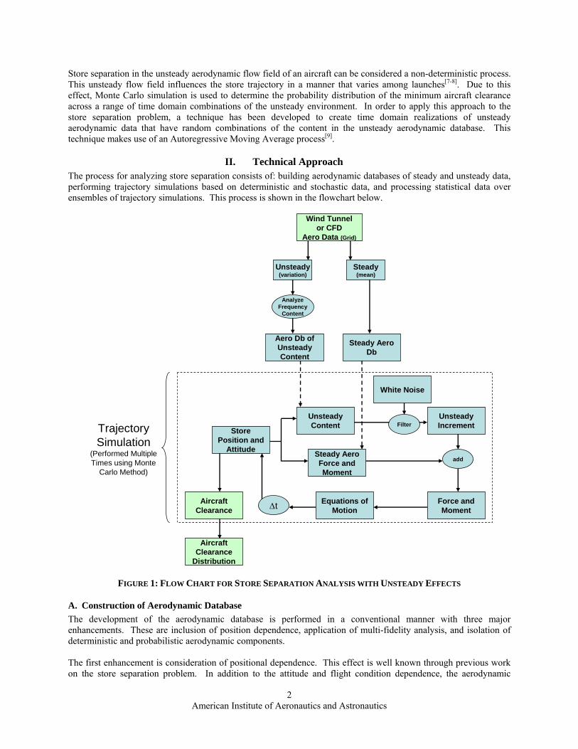
II. Technical Approach The process for analyzing store separation consists of: building aerodynamic databases of steady and unsteady data, performing trajectory simulations based on deterministic and stochastic data, and processing statistical data over ensembles of trajectory simulations. This process is shown in the flowchart below.

Wind Tunnelor CFD

Aero Data (Grid)

Unsteady(variation)

Steady(mean)

Steady Aero Db

AnalyzeFrequency

Content

Unsteady Increment

Force and Moment

Aircraft Clearance

Aero Db of Unsteady Content

Trajectory Simulation

(Performed Multiple Times using Monte

Carlo Method)

Aircraft Clearance

Distribution

Store Position and

Attitude

Unsteady Content

Steady Aero Force and Moment

∆t

White Noise

add

Equations of Motion

Filter

FIGURE 1: FLOW CHART FOR STORE SEPARATION ANALYSIS WITH UNSTEADY EFFECTS

A. Construction of Aerodynamic Database The development of the aerodynamic database is performed in a conventional manner with three major enhancements. These are inclusion of position dependence, application of multi-fidelity analysis, and isolation of deterministic and probabilistic aerodynamic components. The first enhancement is consideration of positional dependence. This effect is well known through previous work on the store separation problem. In addition to the attitude and flight condition dependence, the aerodynamic


3

response is dependent on the position of the store relative to the aircraft flow field. This dependence is captured through performing test and analysis through a grid of store positions. The inclusion of position dependence multiplies the number of data points needed by the number of position samples. While these data points could theoretically all be generated through an exhaustive survey of test points and time accurate CFD runs, a practical consideration shows that the resources required for this type of approach make it infeasible. This leads to a demand for multi-fidelity analysis to make use of limited high-fidelity data gathered from the wind tunnel or high-order CFD analysis along with a comprehensive survey of low-fidelity analyses from empirical methods or potential flow analysis to efficiently construct an aerodynamic database that adequately represents the relevant physics. Additionally, the probabilistic effects should be isolated in this data so that they can be combined using a stochastic method. More detailed description of the proposed methods for multi-fidelity analysis and probabilistic methods are included below.

The aerodynamic database is stored as an Aerodynamic Database Object. This object includes all the tabulated analysis results (both low-fidelity and high-fidelity) at all flight conditions analyzed. Furthermore, the Aerodynamic Database object includes methods that can automatically apply the required high fidelity corrections to the low fidelity data, and interpolate all data across the flight envelope in order to estimate the aerodynamic forces at any possible flight condition. This is a crucial capability, as the aerodynamic database is used to calculate forces due to trimmed flight conditions across a trajectory.

Det

erm

inis

tic T

erm

sPr

obab

ilist

ic T

erm

s

Significant Hi-Fi

Some Hi-Fi Likely Neglected

Very Likely NeglectedSignificant Lo-Fi

Some Lo-Fi

Significant Multi-Fi

Some Multi-Fi

⎪⎪⎪⎪⎪⎪⎪

⎭

⎪⎪⎪⎪⎪⎪⎪

⎬

⎫

⎪⎪⎪⎪⎪⎪⎪

⎩

⎪⎪⎪⎪⎪⎪⎪

⎨

⎧

∆∆∆∆∆∆∆∆∆∆∆

⎥⎥⎥⎥⎥⎥⎥⎥

⎦

⎤

⎢⎢⎢⎢⎢⎢⎢⎢

⎣

⎡

∂∂∂∂∂∂∂∂∂∂∂∂

∂∂∂∂∂∂∂∂∂∂∂∂

∂∂∂∂∂∂∂∂∂∂∂∂

∂∂∂∂∂∂∂∂∂∂∂∂∂∂∂∂∂∂∂∂∂∂∂∂∂∂∂∂∂∂∂∂∂∂∂∂∂∂∂∂∂∂∂∂∂∂∂∂∂∂∂∂∂∂∂∂∂∂∂∂∂∂∂∂∂∂∂∂∂∂∂∂∂∂∂∂∂∂∂∂∂∂∂∂∂∂∂∂∂∂∂∂∂∂∂∂

=

⎪⎪⎪⎪

⎭

⎪⎪⎪⎪

⎬

⎫

⎪⎪⎪⎪

⎩

⎪⎪⎪⎪

⎨

⎧

∆

∆∆∆

∆∆

∞

∞

∞

∞

∞

∞

∞

qMzyxrqp

qMqMqMqFqFqF

MMMMMMMFMFMF

zMzMzMzFzFzF

yMxMrMqMpMMMMyMxMrMqMpMMMMyMxMrMqMpMMMMyFxFrFqFpFFFFyFxFrFqFpFFFFyFxFrFqFpFFFF

M

MMF

FF

z

y

x

z

y

x

z

y

x

z

y

x

z

y

x

z

y

x

zzzzzzzz

yyyyyyyy

xxxxxxxx

zzzzzzzz

yyyyyyyy

xxxxxxxx

z

y

x

z

y

xφβα

φβαφβαφβαφβαφβαφβα

//////

//////

//////

////////////////////////////////////////////////

⎪⎪⎪⎪⎪⎪⎪

⎭

⎪⎪⎪⎪⎪⎪⎪

⎬

⎫

⎪⎪⎪⎪⎪⎪⎪

⎩

⎪⎪⎪⎪⎪⎪⎪

⎨

⎧

∆∆∆∆∆∆∆∆∆∆∆

⎥⎥⎥⎥⎥⎥⎥⎥

⎦

⎤

⎢⎢⎢⎢⎢⎢⎢⎢

⎣

⎡

∂∂∂∂∂∂∂∂∂∂∂∂

∂∂∂∂∂∂∂∂∂∂∂∂

∂∂∂∂∂∂∂∂∂∂∂∂

∂∂∂∂∂∂∂∂∂∂∂∂∂∂∂∂∂∂∂∂∂∂∂∂∂∂∂∂∂∂∂∂∂∂∂∂∂∂∂∂∂∂∂∂∂∂∂∂∂∂∂∂∂∂∂∂∂∂∂∂∂∂∂∂∂∂∂∂∂∂∂∂∂∂∂∂∂∂∂∂∂∂∂∂∂∂∂∂∂∂∂∂∂∂∂∂

+

∞

∞

∞

∞

∞

∞

∞

qMzyxrqp

qMqMqMqFqFqF

MMMMMMMFMFMF

zMzMzMzFzFzF

yMxMrMqMpMMMMyMxMrMqMpMMMMyMxMrMqMpMMMMyFxFrFqFpFFFFyFxFrFqFpFFFFyFxFrFqFpFFFF

z

y

x

z

y

x

z

y

x

z

y

x

z

y

x

z

y

x

zzzzzzzz

yyyyyyyy

xxxxxxxx

zzzzzzzz

yyyyyyyy

xxxxxxxx

φβα

φβαφβαφβαφβαφβαφβα

//////

//////

//////

////////////////////////////////////////////////

FIGURE 2: AERODYNAMIC DATABASE ILLUSTRATING POSITION DEPENDENCE, MULTI-FIDELITY ANALYSIS, AND

PROBABILISTIC TERMS. NOTE THAT LINEARIZED TERMS ARE SHOWN FOR CLARITY WHILE THE ACTUAL DATABASE IS NON-LINEAR.

B. Representing Unsteady Aerodynamic Behavior In order to represent unsteady aerodynamic behavior in the simulation, it needs to be stored in a database as a function of flight condition, attitude, and position for a given time. This time domain realization of the unsteady aerodynamic data must be obtained from frequency domain data since that is the form in which it is stored based on test or CFD data. In order to perform this conversion to the frequency domain in a manner that allows for random combination of the frequency content of the data, an Autoregressive Moving Average (ARMA) Process is used to


4

create linear causal filters. This allows simulations to be performed on aerodynamic conditions with a given frequency content. The filters used are of the form:

∑

∑

=

−

=

−

+== p

k

kk

q

k

kk

za

zb

zAzBzH

1

0

1)()()( .

These filters convert white noise to aerodynamic data using the equation:

∑∑==

−=−+q

kk

p

kk knwbknxanx

01)()()(

where n is the current sample, x(n) is the aerodynamic data of interest and w(n) is the while noise sequence. This data has the same frequency content as the measured data, and includes randomness in the superposition of the frequency content. The fact that this type of filter includes previous response data points allows for autoregressive behavior that avoids non-physical deviations from the preceding time history. It should be noted that these filters are created across the range of available flight conditions creating a database of filters as a function of attitude, position, and flight condition (α, β, φ, x, y, z, M, q).

C. Stochastic Trajectory Simulation With the aerodynamic databases defined, the simulation of a given trajectory becomes a relatively straightforward task. The trajectory is simulated by looking up the forces and moments based on the attitude, position, flight condition, and time. These forces lead to accelerations which are integrated to update the vehicle position and velocity for use in the next time step. This process is iterated through the trajectory. The entire trajectory process is then repeated over an ensemble of combinations of the frequency content of the unsteady data. Once this ensemble of realizations is completed, the mean and standard deviation of the output data are computed. These statistics are taken quantities including the minimum clearance between the store and aircraft to characterize the behavior and uncertainty associated with store separation at a given condition.

III. Demonstration of Unsteady Aerodynamic Representation

A. Initial Verification and Validation Once the filter generation software was written, initial verification and validation was performed on an example frequency response function. In order to perform this initial validation, the frequency response chosen was relatively simple. This included two prominent modes (a narrow mode at 80 Hz and a wider mode at 200 Hz) along with white noise between 0 and 500 Hz. This data was stored with a frequency resolution of 1 Hz. This frequency response function is shown in Figure 3.


5

FIGURE 3: EXAMPLE FREQUENCY RESPONSE FUNCTION.

The example frequency response function was input to the filter development software. The filter was chosen and time domain datasets were obtained by applying the filter to white noise. Time domain results for a high order (p=64) filter are shown in Figure 4 through Figure 6. Figure 5 has been annotated to illustrate evidence of energy at the two prominent modes of the target frequency response function. Note that each of the realizations shown exhibits random behavior with respect to the phasing of the frequency content. Time domain realizations were converted to the frequency domain to verify the accuracy of the frequency content in these datasets. Figure 7 shows a result converted to the frequency domain using Welch’s method of spectral estimation with 1,000 FFTs Hanning windowed with 90% overlap. Note that frequency content of the dataset generated by the filter demonstrates excellent correlation with the target frequency response function. This result was replicated for several realizations of the random sequence.

FIGURE 4: A 200 SEC DATASET GENERATED BY ARMA FILTER.


6

FIGURE 5: A 0.3 SEC EXCERPT ANNOTATED TO HIGHLIGHT ENERGY AT 80 AND 200 HZ.

FIGURE 6: TWO TIME HISTORY EXCERPTS FROM THE SAME FILTER DEMONSTRATING STOCHASTIC BEHAVIOR.

(80 Hz)-1

(200 Hz)-1


7

FIGURE 7: COMPARISON OF FREQUENCY RESPONSE FUNCTION FROM ARMA FILTER TO TARGET

DEMONSTRATING EXCELLENT CORRELATION.

B. Application of Filter to CFD Data The applicability of the ARMA filter method has been tested for use on CFD data for the configuration described below. Lift and moment coefficient data were converted to the frequency domain and filters were designed to fit this data. These filters were verified by developing time domain simulations (at a constant z value) based on these filters. These time histories were then converted to the frequency domain and compared to the frequency response data generated directly from CFD. These results are shown in Figure 8. Excellent correlation is observed between the frequency response functions from the filters and the CFD results. This is an indication that this method is applicable for representing the unsteady aerodynamic data on the store for various positions.


8

Figure 8: Frequency domain comparison of simulation with filters to CFD data.


9

IV. Example Problem Based on MK-82 JDAM Small Scale Drop Testing from a Generic Rectangular Bay

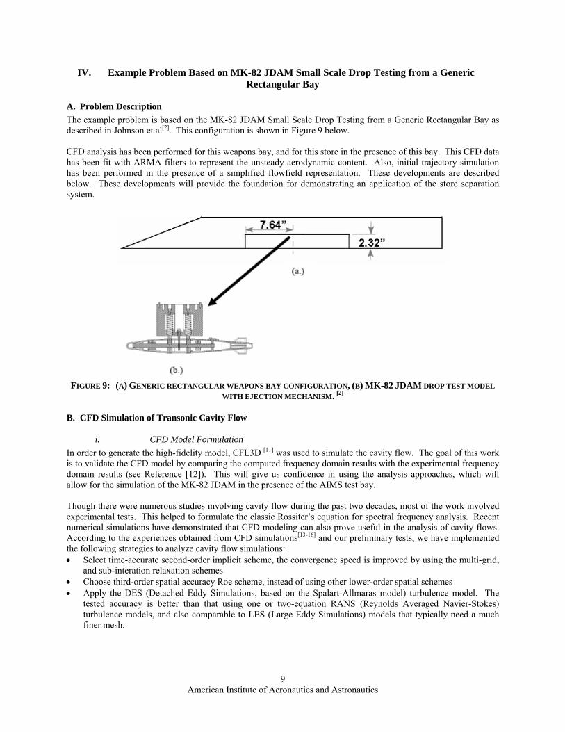
A. Problem Description The example problem is based on the MK-82 JDAM Small Scale Drop Testing from a Generic Rectangular Bay as described in Johnson et al[2]. This configuration is shown in Figure 9 below. CFD analysis has been performed for this weapons bay, and for this store in the presence of this bay. This CFD data has been fit with ARMA filters to represent the unsteady aerodynamic content. Also, initial trajectory simulation has been performed in the presence of a simplified flowfield representation. These developments are described below. These developments will provide the foundation for demonstrating an application of the store separation system.

FIGURE 9: (A) GENERIC RECTANGULAR WEAPONS BAY CONFIGURATION, (B) MK-82 JDAM DROP TEST MODEL

WITH EJECTION MECHANISM. [2]

B. CFD Simulation of Transonic Cavity Flow

i. CFD Model Formulation In order to generate the high-fidelity model, CFL3D [11] was used to simulate the cavity flow. The goal of this work is to validate the CFD model by comparing the computed frequency domain results with the experimental frequency domain results (see Reference [12]). This will give us confidence in using the analysis approaches, which will allow for the simulation of the MK-82 JDAM in the presence of the AIMS test bay. Though there were numerous studies involving cavity flow during the past two decades, most of the work involved experimental tests. This helped to formulate the classic Rossiter’s equation for spectral frequency analysis. Recent numerical simulations have demonstrated that CFD modeling can also prove useful in the analysis of cavity flows. According to the experiences obtained from CFD simulations[13-16] and our preliminary tests, we have implemented the following strategies to analyze cavity flow simulations: • Select time-accurate second-order implicit scheme, the convergence speed is improved by using the multi-grid,

and sub-interation relaxation schemes • Choose third-order spatial accuracy Roe scheme, instead of using other lower-order spatial schemes • Apply the DES (Detached Eddy Simulations, based on the Spalart-Allmaras model) turbulence model. The

tested accuracy is better than that using one or two-equation RANS (Reynolds Averaged Navier-Stokes) turbulence models, and also comparable to LES (Large Eddy Simulations) models that typically need a much finer mesh.


10

ii. Test Detail

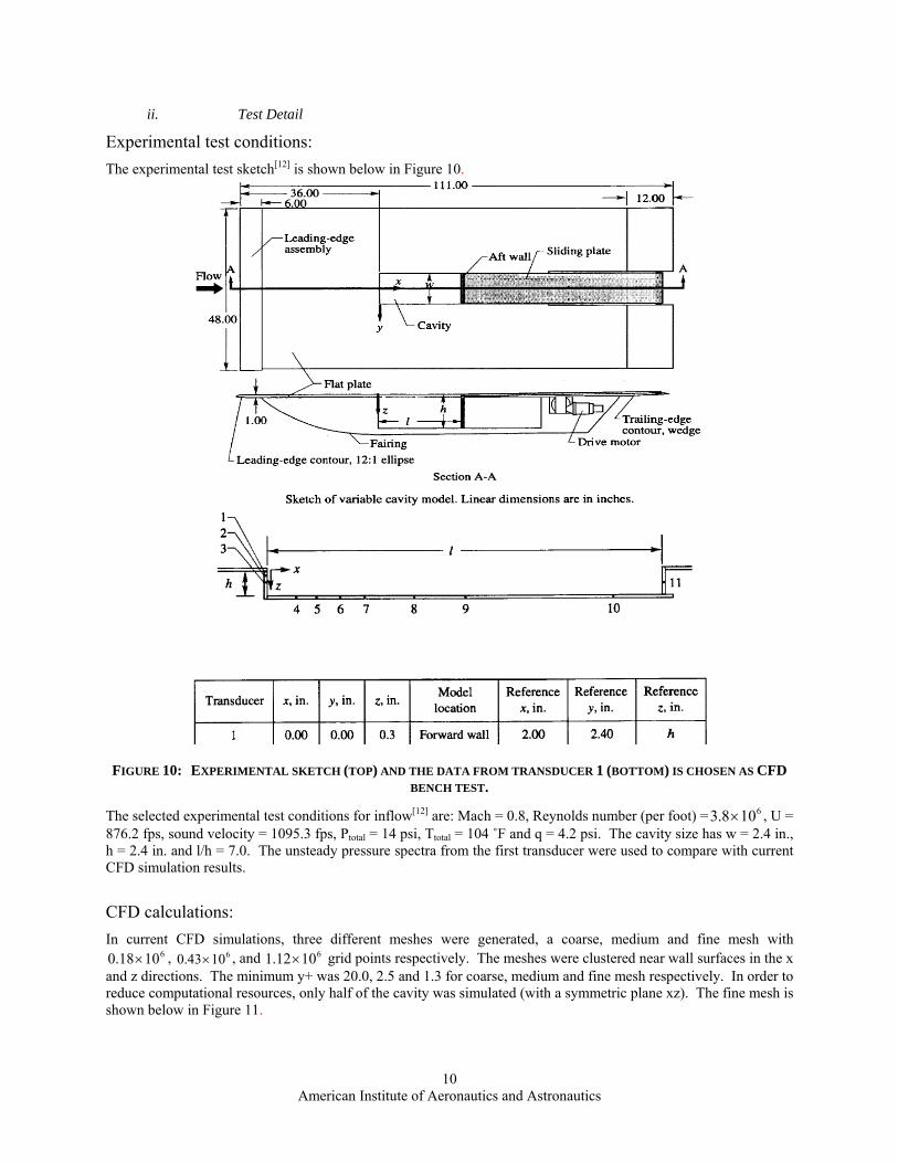
Experimental test conditions: The experimental test sketch[12] is shown below in Figure 10.

FIGURE 10: EXPERIMENTAL SKETCH (TOP) AND THE DATA FROM TRANSDUCER 1 (BOTTOM) IS CHOSEN AS CFD BENCH TEST.

The selected experimental test conditions for inflow[12] are: Mach = 0.8, Reynolds number (per foot) = 6108.3 × , U = 876.2 fps, sound velocity = 1095.3 fps, Ptotal = 14 psi, Ttotal = 104 ˚F and q = 4.2 psi. The cavity size has w = 2.4 in., h = 2.4 in. and l/h = 7.0. The unsteady pressure spectra from the first transducer were used to compare with current CFD simulation results.

CFD calculations: In current CFD simulations, three different meshes were generated, a coarse, medium and fine mesh with

61018.0 × , 61043.0 × , and 61012.1 × grid points respectively. The meshes were clustered near wall surfaces in the x and z directions. The minimum y+ was 20.0, 2.5 and 1.3 for coarse, medium and fine mesh respectively. In order to reduce computational resources, only half of the cavity was simulated (with a symmetric plane xz). The fine mesh is shown below in Figure 11.


11

FIGURE 11: CFD FINE MESH DISTRIBUTION

The estimations in Reference [16] for a DES model indicated that the minimum allowable grid spacing should be 5/λ=∆ , where λ is the sound wave length to capture, and the time step is max/Ut ∆=∆ . These parameters

have been successfully applied to cavity flow simulations as seen in References [13] and [14]. In current numerical

simulations, the wavelength 2000

1095.3== ∞f

aλ = 0.547 ft, and 1094.05/ ==∆ λ ft. The mesh size

requirement has easily satisfied this requirement to secure simulated frequency up to 2000 Hz. Furthermore, the required time step is 4

max 1025.1 876.2/1094.0// −∞ ×==∆=∆=∆ UUt seconds. In order to increase sub-iteration

stability of the unsteady flow simulations, a t∆ of 5100432.3 −× seconds was selected for use in all of the following test cases.

iii. Numerical Test Results The CFD numerical tests have been performed on three levels of mesh densities to examine the results in the frequency domain from transducer 1. The comparison between CFD simulation on the fine mesh and NASA wind tunnel test data[12] is shown in Figure 12.

The numerical test results indicate that the mode frequencies of NASA’s tests are generally well captured in present simulations from coarse to fine meshes except slightly large difference exists in the first mode frequency. The sound pressure level (SPL) spectra from fine mesh in the first six modal frequencies give the best estimations of the SPL data of the experimental tests (see Figure 12), though the medium mesh also presents a good agreement in general. The coarse mesh does not capture the SPL spectra well, especially in the region of high frequencies. The pressure extracted at point 1 from CFD simulation is shown in Figure 13 in the time domain. The midspan plane pressure, Mach number, and vorticity contours at two specified time points (t = 0.055 and t = 0.06 sec) indicated by red dash lines in Figure 13) are shown in Figure 14 through Figure 16 on mid-span plane. Significant differences in pressure and Mach number distributions are observed at the two time points. At t = 0.055 a large recirculation zone exists within the cavity. In Figure 16, the non-dimensional vorticity contours on the mid-span plane at two time points are presented, the vortices (in red color) generated from leading edge shear layer of the cavity are small compared with the cavity size which are shed at the leading edge of the cavity mouth and dissipate at the rear of the cavity. The cavity flow demonstrates a broadband spectrum and a more complicated mechanism than a simple shear layer mode. This phenomenon corresponds well to the numerical flow results[13].


12

FIGURE 12: SPL VS. FREQUENCY (FINE MESH)

FIGURE 13: PRESSURE VS. TIME FROM TEST POINT 1 (FINE MESH)


13

FIGURE 14: PRESSURE (PSI) CONTOURS AT TIME = 0.055 SEC (UPPER)

AND TIME = 0.060 SEC (BOTTOM)

FIGURE 15: MACH NUMBER CONTOURS AT TIME = 0.055 SEC (UPPER)



14

FIGURE 16: VORTICITY (NORMALIZED) CONTOURS AT TIME = 0.055 SEC (UPPER)


To perform cross validations, a semi-empirical method, known as the Rossiter equation, was examined. The modified version of Rossiter’s equation, which is valid for a wide range of March numbers is expressed as:

vkMM

mfreq1)

211( 2/12 +

−+

−=

−∞∞

γξ

where m = 1,2,3, … for each mode, and ξ , a function of l/h and vk , varies with the ∞M (= 0.4 – 1.2); from Reference [24] the ξ vs. l/h relation is given in Table 1. In current test case we choose γ = 1.4, ξ = 0.46 and

vk = 0.57.

TABLE 1: ξ VS. L/H

l/h 4 6 8 10 ξ 0.25 0.38 0.54 0.58

The Rossiter equation, based on two-dimensional cavity flow assumption, can only predict possible frequencies; it does not predict the amplitudes of the mode or identify the dominant mode. The estimations of modal frequencies, based on current flight conditions and cavity size, are listed in Table 2. The frequencies, except the first mode, compare reasonably well with the experimental test results. The SPL magnitude data, tabulated in Table 3, is also in good agreement with experimental results.


15

TABLE 2: MODEL FREQUENCY (HZ) COMPARISON

Mode 1 2 3 4 5 6 Experiment 115 390 710 980 1230 1550 CFD fine 70.0 394 723 1051 1281 1577 CFD medium 97.0 340 777 1020 1312 1555 CFD coarse 68.6 377 687 1039 1236 1510 Rossiter 139.0 398.0 657 915 1174 1433

TABLE 3: MODEL SPL (DB) COMPARISON

Mode 1 2 3 4 5 6 Experiment 138 134 132 130 128 125 CFD fine 147 139 134 132 129 127 CFD medium 150 137 139 138 130 125 CFD coarse 157 131 129 115 101 95 Rossiter NA NA NA NA NA NA

iv. Conclusion Regarding Transonic Cavity Flow Analysis Comparison studies among experimental, analytical and numerical tests have proven current CFD implementation as an effective tool for high-fidelity cavity flow modeling. The CFD tests provided both frequencies and amplitudes in good agreement with experimental test results. In the next section, we will further examine the unsteady flow interaction between cavity and store. This will include aerodynamics forces on the store at various locations within the cavity flow field.

C. CFD Simulation of Forces on Store in Presence of Transonic Cavity Flow

i. CFD Model Formulation In this section, the store aerodynamic loads, in the presence of the cavity flow field will be examined. The same CFD simulation strategies and parameters implemented in previous section have been chosen. This includes the time-accurate second-order implicit scheme, the third-order spatial accuracy Roe scheme and the DES turbulence model. In order to facilitate the numerical simulations of the store at various positions below the cavity, a parametric mesh generator for the model scale MK82-JDAM configuration has been developed. This provides the user with a powerful tool, which reduces the turn-around time associated with moving the store to other test positions, generating the new meshes and preparing CFD input files. In order to test current CFD program, we employed the MK-82 JDAM small scale wind tunnel model[2][10] as a bench test model. The meshes were generated with 22 blocks are illustrated in Figure 17, in which center of gravity (Zcg) of the store is located at z = 1.4 in relative to the test bay, where z is in the wind tunnel coordinate system (z positive down). This is consistent with the wind tunnel test data. 61061.1 × grid points were used for the test at z = 1.4 in. The grid points were increased up to 6102.2 × for the z = 6.4 in test.


16

FIGURE 17: MK-82 JDAM WIND TUNNEL MODEL: CFD VOLUME MESHES (LEFT) AND SURFACE MESHES OF

CAVITY AND STORE (RIGHT), ONLY A HALF OF CONFIGURATION SIMULATED

ii. MK-82 JDAM Test Results To compare with the wind tunnel test results, the inflow conditions in CFD simulations have been extracted from wind tunnel test conditions in Table 11 and 14 of Reference [10]. They are listed below: • Mach number: 0.8 • Re (1/ inch): 0.2025E+06 • T(R): 560.00 • Sref (in^2): 0.9076 • Cref (in): 1.0750 • Bref (in): 1.0750 • Xmc (in): 27.860 (=Xcg) • Ymc (in): 0.0 (=Ycg) • Zmc (in): 1.4 to 6.4 (=Zcg) • Angle of attack: 0.0

The CFD simulations were performed at different z locations, below the cavity, using the same conditions as in the wind tunnel tests. The time step for unsteady flow simulation, which was chosen based on the previous cavity flow simulations, was set to be 5108722.2 −×=∆t . This corresponds to the non-dimensional dt = 0.4 in running CFL3D. In all simulations the sting is not included in the CFD model. The CFD numerical test results for the zero angle of attack store model are plotted (see Figure 18) against the wind tunnel tests[10] and numerical tests from BCFD (Boeing’s CFD tests[10]). The CFD results, which are based on the mean results (time averaged) of the unsteady forces/moments, compare well with the wind tunnel tests (red line). This provides a good estimation in both trends and quantities for the normal force and the pitching moment (Cn and Cm) on the store at the different locations. As demonstrated in Reference [10], Boeing’s numerical tests using BCFD (black line), which use a quasi-steady assumption, yield poor estimations of the wind tunnel measurements (Cn and Cm). This suggests that the quasi-steady state assumption is insufficient for a flow field simulation which includes store separation. The differences of Cm between the CFD simulations and wind tunnel tests are observed in Figure 18. One possible source of error results from the CFD model which does not include the protuberance on the aft portion of the MK-82 JDAM and the canards on the front surface of the store (see Figure 17 and Figure 19). Another potential influence may come from the sting in wind tunnel tests. The numerical tests at zero angle of attack (pitch angle 0.0) from Boeing’s BCFD indicate the differences were not significant. However, as the BCFD results are inaccurate, it is difficult to determine what the effect of the sting is on the store loads, see Reference [10], section 3.3.3 for more details.


17

FIGURE 18: COMPARISONS OF PRESENT CFD TESTS (CN AND CM VS. Z) WITH THE WIND TUNNEL

AND BCFD RESULTS

FIGURE 19: PRESSURE DISTRIBUTION CONTOURS (PSI) AND STREAMLINES: Z =1.4 IN (LEFT) AND Z =6.4 IN (RIGHT)

In Figure 19 the streamlines and pressure contours (psi) of the store (on the x-z symmetric plan) are shown at two different locations z = 1.4 in and z = 6.4 in. This shows that the store has a strong influence on the flow field near the bay and does not have a strong influence far from the bay. Also note that the rear fins (stabilizers) are invisible as they are located on the planes 45 degrees away from the x-z symmetric plane. The results, which illustrate the Cn and Cm vs. time history are plotted in Figure 20 (for z = 1.4 in and 6.4 in). As mentioned above, the mean (time-averaged) Cn and Cm results from Figure 20 have been plotted in Figure 18. This compares well with the wind tunnel tests. These variation histories include Cn, Cm, and Cd (not shown) vs. time are vital and will be used to further trajectory predictions for the store separation.


18

FIGURE 20: CN AND CM VS. TIME FOR THE STORE AT Z =1.4 IN (UPPER) AND Z =6.4 IN (BOTTOM)

Finally, in order to quantitatively analyze the variation of the Cn and Cm magnitudes in their whole time history, we collected the data from test cases in Figure 20, and plotted the probability density functions and the cumulative distribution functions in Figure 21. The normal probability distributions of the forces and moments (by curve fitting) are shown in red lines. The data at z = 1.4 in. does not fit well using a normal distribution. In Figure 21 we can easily indentify the differences of µ (mean values) and σ (standard deviations) between z = 1.4 in and 6.4 in. The values of µ and σ decrease with increasing z. If choosing the 6σ as the range of probability distribution, at z = 1.4 in. the Cm and Cn are in the range of -1.08 to 3.755 and -0.85 to 0.376 respectively. These variations are significant compared to the mean values of Cm (1.34) and Cn (-0.242). The µ and σ values at different locations also provide useful information, which may be used in future trajectory predictions.


19

CN AT Z=1.4: µ =- 0.242, σ = 0.206 CM AT Z = 1.4: µ = 1.34, σ = 0.805

CN AT Z = 6.4: µ = - 0.153, σ = 0.0695 CM AT Z = 6.4: µ = 0.506, σ = 0.286

FIGURE 21: CN AND CM PROBABILITY DISTRIBUTIONS AT Z =1.4 IN (UPPER) AND Z =6.4 IN (BOTTOM)

iii. Conclusion Regarding Unsteady Store Forces In this section, the CFD model was validated against the available wind tunnel measurements in the presence of store in cavity flow. The good correlation between CFD and wind tunnel tests indicate that the proposed strategies are reasonable, though the sources of error need to be identified in the future work. This includes the CFD model accuracy and the effect of sting. It can be concluded that the steady-state assumption for CFD simulations, which was adopted by Boeing[10] is unsuitable to simulate the strong unsteady flow with the interaction between cavity (bay) and store. The steady-state method generally uses schemes without considering time-accuracy, such as the large time steps, various local time steps, furthermore, the first order time schemes may result in information losses and the suppression of the flow property variations. So far, the numerical tests were performed on the CFD models with the structured mesh, however the unstructured mesh model is not out of our version. The major issue is that we generally have more confidence on the turbulence model implemented in structured mesh than that in unstructured mesh. In order to choose a reliable turbulence model, it is suggested that any CFD code with either structure mesh or unstructured mesh needs to perform a bench test, such as the cavity flow case without the store in previous section. The current numerical simulations can be further applied to supplement or replace wind tunnel tests for the mean results (time averaged) of the forces and moments, and moreover provide their variations (µ and σ) along the time histories, which are not available from wind tunnel tests. The applications of CFD test results in predicting the stochastic trajectories will be given in the following section.


20

D. Stochastic Trajectory Simulation Initial demonstration of stochastic trajectory simulation has been performed. The simulations combined a freestream aerodynamic database with aerodynamic increments due to both steady and unsteady bay effects. The unsteady bay effects were determined using time accurate CFD analysis. The simulation results are compared among solutions with no unsteady effects and an ensemble of 100 realizations solved with unsteady aerodynamic effects (Figure 22,23). These results are compared to the test data from Reference [2] in Figure 24. Reasonable correlation is observed, however the simulation results are consistently lower than the test data. This is likely due to inaccuracy in the steady aerodynamic database. Other possible explanations include the use of an insufficient number of unsteady aerodynamic data points. As an initial validation of the unsteady content in the simulation, the frequency response data in two of the simulations are compared to the spectral data in the unsteady aerodynamic database. This comparison is shown in Figure 25 and shows spectral data on the same order as the points in the database.

FIGURE 22: STOCHASTIC SIMULATION OF EXAMPLE PROBLEM


21

FIGURE 23: STOCHASTIC SIMULATION OF EXAMPLE PROBLEM - ALPHA VS TIME

Comparison of RUSAT to Wind Tunnel

-15

-10

-5

0

0 5 10 15

X (in)

Z (in

)

Run 1 - 6D Photo Run 2 - 6D PhotoRun 3 - 6D Photo Run 4 - 6D PhotoRun 11 - 6D Photo Run 1 - 3D PhotoRun 2 - 3D Photo Run 3 - 3D PhotoRun 4 - 3D Photo Run 11 - 3D PhotoSteady RUSAT result RUSAT 2RUSAT 4

FIGURE 24: COMPARISON OF RUSAT SIMULATION TO TEST DATA


22

0.1

1

10

100

0 200 400 600 800 1000 1200 1400 1600 1800 2000

Freq

uency Respon

se Fu

nction

(CM)

Frequency (Hz)

Comparison of Frequency Response Magnitudes

z=1.4

z=3.4

z=5.4

z=6.4

Run1

Run2

FIGURE 25: COMPARISON OF SPECTRAL CONTENT FROM SIMULATION TO UNSTEADY DATABASE

V. Identification of example configurations susceptible to store separation bifurcations due to unsteady flow

An objective of this system is identification of example configurations susceptible to store separation bifurcations due to unsteady flow. As an initial study, this is accomplished by performing a sensitivity study for the JDAM MK-82 example problem. This sensitivity investigates the effect of variation in the vehicle CG on the likelihood of collision with a notional parent bay. For this example case, collision is defined as any point in the trajectory with z greater than zero for values of x between 5 and 20. An ensemble of 50 simulations was run for each of the vehicle configurations (CG locations) in this study. It is acknowledged that this is a relatively simple example problem, however it is an important capability demonstration of the type of study that can be performed using RUSAT. The results of this study are shown in Figure 26. As expected, stores with CG locations further aft are found to be more likely to collide with the parent bay.

0102030405060708090

100

0 0.1 0.2 0.3 0.4 0.5 0.6

Likelihoo

d of Collision (%

)

Change in CG Relative to Baseline (calibers) (+ aft)

Effect of CG Location on Likelihood of Collision in Unsteady Flow Enviroment for Example Problem

FIGURE 26: LIKELIHOOD OF COLLISION AS A FUNCTION OF CG LOCATION FOR EXAMPLE PROBLEM


23

VI. Conclusion A new method has been developed for analyzing the response of a store to steady and unsteady aerodynamic effects. This method considers an ensemble of trajectories with random release time relative to the state of the unsteady aerodynamic flow field. This method has been demonstrated on an example application and significant deviation in store trajectories has been observed. These demonstration results have been compared to test data. Reasonable correlation has been observed and possible explanations for discrepancies have been identified. The method has been developed into a software system known as the Rapid Unsteady Store Analysis Tool (RUSAT).

VII. Acknowledgement Funding for this development has been provided by the Weapons Integration Team of the Air Vehicles Directorate at the Air Force Research Laboratory. The Air Force technical monitor is Rudy Johnson.

VIII. References

1. Arnold, R. J. and Epstein, C. S., “AGARD Flight Test Techniques Series. Volume 5. Store Separation Flight Testing,” AGARD-AG-300-VOL-5, Advisory Group for Aerospace Research and Development, Neuilly-Sur-Seine, France, Apr 1986. Available online from DTIC, ADA171301.

2. Johnson, R., Stanek, M. and Grove , J. “Store Separation Trajectory Deviations due to Unsteady Weapons Bay Aerodynamics,” AIAA-2008-188, 46th AIAA Aerospace Sciences Meeting and Exhibit, Reno, Nevada, Jan. 7-10, 2008.

3. Freeman, J. A., “Applied Computational Fluid Dynamics for Aircraft-Store Design, Analysis and Compatibility,” 44th AIAA Aerospace Sciences Meeting and Exhibit, AIAA 2006-456, 9 - 12 January 2006, Reno, Nevada.

4. Murman, S. M., Aflosmis, M. J. and Berger, M. J., “Simulations of Store Separation from an F/A-18 with a Cartesian Method,” Journal of Aircraft. Vol. 41, no. 4, pp. 870-878. July-Aug. 2004.

5. Jordan, J. K. and Denny, A. G., “Approximation Methods for Computational Trajectory Predictions of a Store Released from a Bay,” AIAA-1997-2201, Applied Aerodynamics Conference, Atlanta, GA, June 1997.

6. Baker, M. L., Munson, M. J., Hoppus, G. W., and Alston, K. Y., “Integrated Hypersonic Aeromechanics Tool (IHAT), Build 4,” AIAA Multidisciplinary Analysis and Optimization Conference, Albany, NY Sept 2004.

7. Johnson, R. A., Stanek, M. J. and Grove, J. E., “Store Separation Trajectory Deviations Due to Unsteady Weapons Bay Aerodynamics,” The Dayton-Cincinnati Aerospace Sciences Symposium, Dayton, OH, March 6, 2007.

8. Coleman, L. A., “F-111/Small Smart Bomb Trajectory Predictions for Safe Separation Analysis using Computational Fluid Dynamics,” Aircraft-Stores Compatibility Symposium, Destin, FL, March 5 - 8, 2001.

9. Proakis, J. G., and Manolakis, D. K., Digital Signal Processing, Prentice Hall, 4th Edition, 2006. 10. Cary, A. C. and Wesley, L. P., “Airframe Integration of Modern Stores (AIMS), Delivery Order 0031: Phase II

& III Analytical Predictions & Validation Testing,” Air Force Research Lab, Dayton, OH, January 2006, AFRL-VA-WP-TR-2006-3079.

11. “CFL3D (Version 5.0) User's Manual,” NASA Langley Research Center. and CFL3D Version 6.4 - General Usage and Aeroelastic Analysis - NASA/TM-2006-214301, April 2006.

12. Maureen B. T. and Plentovich, E.B., “Cavity Unsteady-Pressure Measurements at Subsonic and Transonic Speeds,” NASA TP 3996, December 1997.

13. Li, Z. and Hamed, A., “Numerical Simulation of Sidewall Effects on the Acoustic Field in Transonic Cavity,” AIAA paper 2007-1456, Jan., Reno, NV.

14. Hamed, A., Basu, D. and Das, K., “Assessment of Hybrid Turbulence Models for Unsteady High Speed Separated Flow Prediction,” AIAA paper 2004 - 0684, Jan., Reno, NV.

15. Nayyar, P., Barakos, G.N. and Badcock, K.J., “CFD Analysis of Transonic Cavity Flow using DES and LES,” CFD Laboratory, University of Glasgow, Symposium on Hybrid RANS-LES Methods, Stockholm, July 2005.

16. Spalart, P.R., “Young-Person’s Guide to Detached-Eddy Simulation Grids,” NASA CR 2001-211032.

A System for Simulation of Store Separation Including ...

Documents

Transcript of A System for Simulation of Store Separation Including ...