The Pennsylvania State University

The Graduate School

Department of Geography

A SYNOPTIC CLIMATOLOGY OF CONTRAIL OUTBREAKS AND ASSOCIATED

SURFACE TEMPERATURE IMPACTS FOR TWO SUB-REGIONS OF THE

CONTINENTAL UNITED STATES

A Thesis in

Geography

by

Jase E. Bernhardt

2013 Jase E. Bernhardt

Submitted in Partial Fulfillment

of the Requirements

for the Degree of

Master of Science

May 2013

The thesis of Jase Bernhardt was reviewed and approved* by the following:

Andrew Carleton

Professor of Geography

Thesis Advisor

Brent Yarnal

Professor of Geography & Associate Department Head

Karl Zimmerer

Professor of Geography

Head of the Department of Geography

*Signatures are on file in the Graduate School

iii

ABSTRACT

The artificial cloudiness, or “contrail cirrus,” that results from multiple jet contrail

outbreaks can last for several hours and alter the radiation budget and, thereby, surface

temperatures. An extensive database of satellite-derived “clear-sky” contrail outbreaks over two

regions of the continental United States – the South and the Midwest – for two mid-season

months of 2008 and 2009 was used to determine the potential climatic impact of contrail

outbreaks on surface temperature. Events spanning at least one half of the diurnal cycle of

temperature and covering at least 10,000 km2 were selected for study. The aggregated impact of

outbreaks on maximum and minimum temperatures and on the diurnal temperature range (DTR)

was determined by comparing the departures at stations overlain by outbreaks with those at

adjacent stations having similar synoptic and land surface conditions, but not experiencing

contrail cloudiness. A synoptic climatology (i.e., composite average) of upper troposphere (UT)

variables (temperatures, specific humidity, horizontal winds, and vertical lapse rate) for these

longer-lasting jet contrail outbreaks was also developed to link the impacts of contrail outbreaks

with conditions favorable for their formation. The results at the South stations during the month

of January and the Midwest stations during the month of April both indicate a statistically

significant suppression of DTR at outbreak stations versus adjacent non-outbreak stations. The

South outbreaks generally covered a larger area, occurred in conjunction with an anomalously

cooler UT, and were more likely to take place in a region of warm air advection. Moreover, large

wind shear values and strong gradients of the aforementioned UT variables across the outbreak

box, symptomatic of a baroclinic environment, characterize the formation of the long-lived

contrail outbreaks. The results of this study demonstrate the impact jet contrails have on short-

term weather and climate through the reduction of DTR. The findings can also be used to assist

iv

with the development of a system for real-time forecasting of jet contrails based on the UT

conditions present.

v

TABLE OF CONTENTS

LIST OF FIGURES ................................................................................................................. vi

LIST OF TABLES ................................................................................................................... viii

ACKNOWLEDGMENTS ....................................................................................................... viiii

Chapter 1 Introduction ............................................................................................................ 1

Formation and Observation of Jet Contrail Outbreaks ..................................................... 1

Potential Climatic Impacts of Jet Contrail Outbreaks ...................................................... 5

Chapter 2 Data and Methodologies ......................................................................................... 10

The Outbreaks .................................................................................................................. 10

Selection of Station Pairs for DTR Comparison .............................................................. 16

NARR Data and Development of the Composite Synoptic Environmental Conditions .. 18

Chapter 3 DTR Impacts of Longer-Lived Jet Contrail Outbreaks .......................................... 23

Chapter 4 Synoptic Climatology of Longer-Lived Jet Contrail Outbreaks ............................ 27

The South January 2008 and 2009 Jet Contrail Outbreaks .............................................. 27

The Midwest April 2008 and 2009 Jet Contrail Outbreaks ............................................. 37

Comparison of the January South and April Midwest Outbreak UT Conditions ............ 46

Chapter 5 Summary, Discussion, and Conclusions ................................................................ 49

Appendix A Sample 500 mb Geopotential Height Imagery ................................................... 57

Appendix B Sample Upper Tropospheric Wind Shear Imagery ............................................. 60

vi

LIST OF FIGURES

Figure 1-1: September 11th – 14

th, 2001 DTR anomalies (a) and mean frequency of

contrails for October 1977-79 and 2000-01 (b) ............................................................... 3

Figure 1-2: Satellite-derived changes in contrail frequency between 1977-79 and 2000-

02, normalized to every 100 images ................................................................................ 8

Figure 2-1: Regions of higher contrail outbreak frequency, January 2000-02 ........................ 11

Figure 2-2: Regions of higher contrail outbreak frequency, April 2000-02 ........................... 12

Figure 2-3: January 2009 outbreak frequency anomaly (departure from January 2000-02

averages) ......................................................................................................................... 12

Figure 2-4: April 2009 outbreak frequency anomaly (departure from April 2000-02

averages) ......................................................................................................................... 13

Figure 2-5: Starting times of jet contrail outbreaks selected .................................................. 15

Figure 2-6: Locations of bounding boxes for January 2008 and 2009 longer-lived

outbreaks ......................................................................................................................... 16

Figure 2-7: Locations of bounding boxes for April 2008 and 2009 longer-lived outbreaks .. 17

Figure 2-8: Locations of central outbreak box for January 2008 and 2009 outbreaks in

relation to all outbreak bounding boxes ........................................................................... 21

Figure 2-9: Locations of central outbreak box for April 2008 and 2009 outbreaks in

relation to all outbreak bounding boxes ........................................................................... 22

Figure 4-1: 250 mb temperature composite for January South region outbreaks. .................. 30

Figure 4-2: 250 mb temperature composite anomaly for January South region outbreaks ..... 30

Figure 4-3: 250 mb zonal wind composite for January South region outbreaks...................... 31

Figure 4-4: 250 mb zonal wind composite anomaly for January South region outbreaks. ...... 31

Figure 4-5: 250 mb specific humidity composite anomaly for January South region

outbreaks. ......................................................................................................................... 32

Figure 4-6: Sample 200 mb temperature gradient for 1/8/09 outbreak .................................... 33

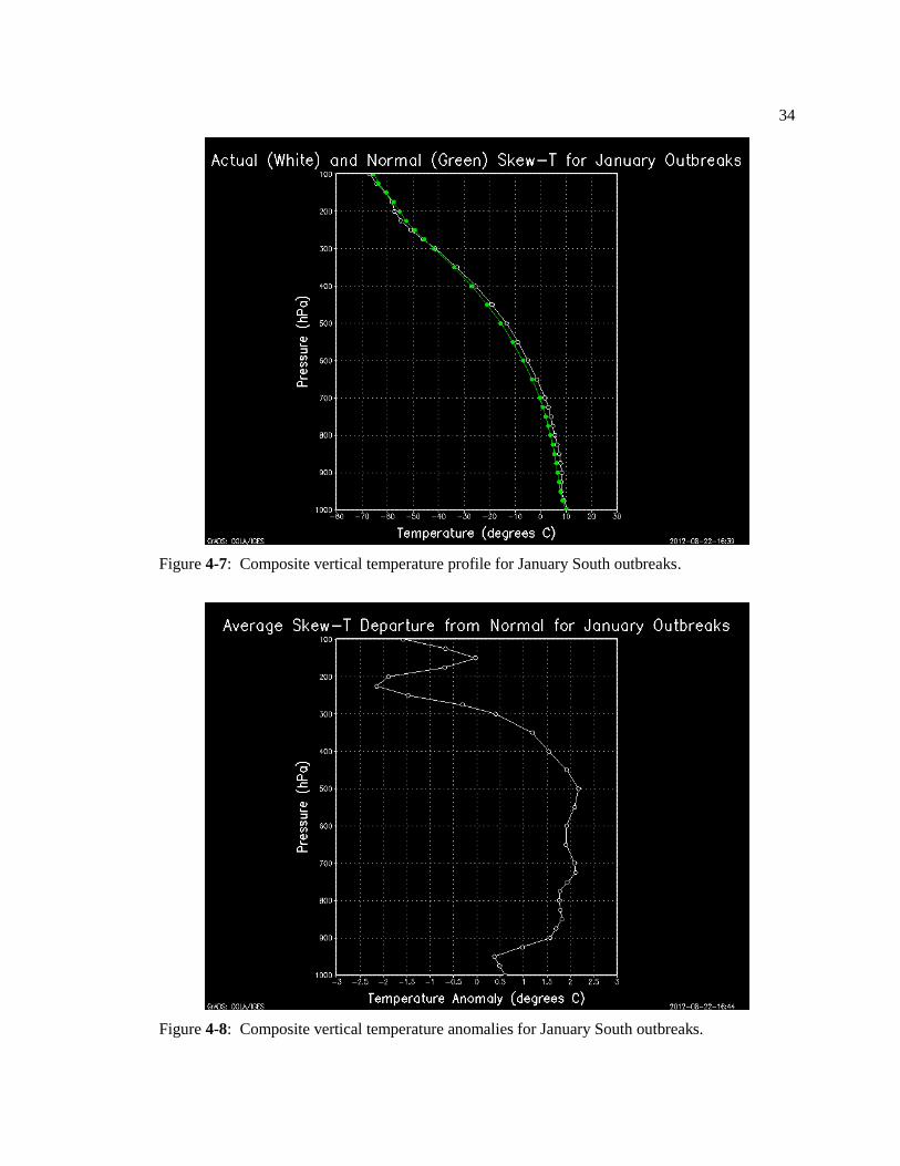
Figure 4-7: Composite vertical temperature profile for January South outbreaks. .................. 34

vii

Figure 4-8: Composite vertical temperature anomalies for January South outbreaks ............. 34

Figure 4-9: Composite vertical zonal wind profile for January South outbreaks. ................... 35

Figure 4-10: Composite vertical zonal wind anomalies for January South outbreaks. ............ 35

Figure 4-11: 250 mb temperature composite for April Midwest region outbreaks. ............... 40

Figure 4-12: 250 mb temperature composite anomaly for April Midwest region outbreaks ... 40

Figure 4-13: 250 mb zonal wind composite for April Midwest region outbreaks. .................. 41

Figure 4-14: 250 mb zonal wind composite anomaly for April Midwest region outbreaks. ... 41

Figure 4-15: 250 mb specific humidity composite anomaly for April Midwest region

outbreaks. ......................................................................................................................... 42

Figure 4-16: Composite vertical temperature profile for April Midwest outbreaks. ............... 43

Figure 4-17: Composite vertical temperature anomalies for April Midwest outbreaks ........... 44

Figure 4-18: Composite vertical zonal wind profile for April Midwest outbreaks. ................. 44

Figure 4-19: Composite vertical zonal wind anomalies for April Midwest outbreaks. ........... 45

viii

LIST OF TABLES

Table 2-1: Information for the selected longer-lived jet contrail outbreaks analyzed in

this study .......................................................................................................................... 14

Table 3-1: DTR impacts of longer-lived jet contrail outbreaks. ............................................. 24

Table 3-2: Composite DTR impacts of jet contrail outbreaks ................................................ 26

Table 3-3: Composite DTR Impacts of days before and after jet contrail outbreaks .............. 26

Table 4-1: Composite horizontal gradients of UT variables for January South region

outbreaks .......................................................................................................................... 32

Table 4-2: Composite station UT data for January South region outbreaks ........................... 33

Table 4-3: Synoptic analysis of January South outbreaks ...................................................... 36

Table 4-4: Composite horizontal gradients of UT variables for April Midwest region

outbreaks .......................................................................................................................... 42

Table 4-5: Composite station UT data for April Midwest region outbreaks .......................... 43

Table 4-6: Synoptic analysis of April Midwest outbreaks ...................................................... 45

ix

ACKNOWLEDGMENTS

I am deeply indebted to my advisor, Andrew Carleton, for his close guidance throughout

the process of completing this thesis. I would also like to thank the other members of my

committee, Brent Yarnal and Paul Knight, for their valuable insights, as well as Sonia Miller for

her technical assistance. Partial funding for this research was provided by National Science

Foundation grants 0819396 and 0819416.

Chapter 1

Introduction

Particularly since the Industrial Revolution, humans have exerted a significant influence

on global climate. The most important anthropogenic influence on surface temperature has been

the emissions of greenhouse gases, as well as of various types of aerosols. However, society has

also had other, more subtle – but still detectable – effects on Earth’s climate system. Among these

additional impacts are land use- land cover changes and jet aviation contrails. Aviation wields a

dual influence on climate, as planes emit greenhouse gases and also initiate artificial cirrus-like

clouds known as contrails (Lee et al. 2009). Although the impacts of contrails are not as well

understood or studied as greenhouse gases, it is generally accepted that they contribute to

regional-scale and global warming. In addition, numerous papers have suggested that contrails

reduce diurnal temperature range (DTR), which could have both beneficial and detrimental

influences on society. This chapter summarizes the impacts of jet contrails on the climate system.

The discussion identifies the key gaps in our understanding of contrail-climate impacts, including

those lacunae that form the basis of this thesis research.

Formation and Observation of Jet Contrail Outbreaks

Contrails are the condensation trails left by jet engines as they release heated, moist

particles and water vapor into the far colder ambient upper troposphere (UT). The plane’s engines

create turbulence, mixing these two types of air together. If the ambient atmosphere is sufficiently

humid, contrails form in narrow lines following the path of the jet. When the atmosphere is

relatively humid, contrails have the potential to last for several hours, slowly spreading due to the

shear associated with the jet stream. In a less humid UT, contrails may last only briefly, or not be

2

produced at all. Hence, jet contrails can be an indicator of the general state of the UT. If contrails

do not form, then there is likely dry air and stable conditions present in the UT, but if they do

form and persist, the UT is likely at or near saturation and less stable, sometime in conjunction

with a trough or cyclone. Contrails are not unique to one geographical area as they can form just

about anywhere, although they are obviously more common in areas of frequent jet traffic, such

as portions of the United States (U.S.) and Europe (National Weather Service, 2011).

A few case studies have shown that contrails have been of historical importance (e.g.,

Ryan et al. 2011; Travis et al. 2004). One of the first examples of widespread jet contrails

occurred during World War II. At that time, commercial air travel was not common, so the high

number of military aircraft involved in allied bombing raids over Europe was highly anomalous.

When synoptic weather conditions were favorable, extensive contrails were observed over

southeastern England, which served as the launching pad for these bombing missions. The

contrails remained for up to several hours, which resulted in a suppressed diurnal temperature

range (DTR) at the surface. This statistically significant reduction in DTR was only found in

locations overflown by a high volume of aircraft, showing that contrails were responsible (Ryan

et al. 2011).

Another instance of historic events playing a role in contrails research, particularly the

potential role in suppressing DTR, was the grounding of commercial aviation in the U.S. after the

attacks of September 11th, 2001. The lack of flights was especially significant over heavily

trafficked regions of the U.S., such as the Midwest. Although tragic, this event presented an ideal

opportunity for climate researchers (Travis et al. 2004). During the three days after the attacks

when no flights occurred, conditions favorable for contrail development existed over the Midwest

and other U.S. sub-regions. Indeed, in the absence of contrails, a statistically significant increase

in DTR was observed not only in this region, but also in portions of the Northeast and

3

Intermountain West (Figure 1-1) – all areas that would have seen contrails had planes been flying

as normal. Interestingly, in the post-9/11 case, it was found that maximum temperatures were

more affected by the lack of contrails than were minimum temperatures. This finding seems

logical as air traffic frequencies are highest during the day, so the lack of any contrails would

result in a larger impact than at night. Daytime temperatures would further be increased due to the

reduction in planetary albedo caused by the reduction in high clouds. Additionally, the research

confirmed that jet contrails most often form in advance of frontal cyclones and convective storms

due to the moistening of the UT at the leading edge of these systems (DeGrand et al. 2000; Travis

et al. 2004).

Jet contrails can be easily visible from the surface during the day, unless obstructed by a

significant amount of low and mid- levels clouds. Similarly, the linear cloud formations

Figure 1-1: September 11th – 14

th, 2001 DTR anomalies (a) and mean frequency of contrails for

October 1977-79 and 200-01 (b) (Travis et al. 2004).

4

characteristic of newly-formed contrails are highly discernible on different types of satellite

imagery, primarily in the visible and infrared (IR) portions of the spectrum, with the IR being the

more useful to researchers because it can be used at any time of day (Carleton and Lamb 1986).

IR imagery also has the advantage of being able to highlight contrails due to their very low

temperatures of below -45 oC (given a location in the upper atmosphere). Persisting contrails –

features that thin vertically and spread laterally – are those contrails most likely to be seen on

satellite images, and also to have the greatest impact on DTR. In these contrails, the “cloud

greenhouse” effect may outweigh the cloud albedo affect, potentially leading to a net surface

warming (as compared to clear-sky conditions). Furthermore, contrails can usually be

distinguished from natural cirrus on satellite IR imagery as they are often shorter and oriented in

different directions from their natural counterparts. Haphazard, intersecting patterns of multiple

linear contrails known as outbreaks also indicate persisting contrails in an area of high jet traffic,

Satellite studies of persisting contrails have also revealed other notable features of outbreaks.

Outbreaks tend to form in groups on meso- or synoptic- scales, and may recur over several days

while conditions remain favorable (Carleton et al. 2008). Satellite observations also confirm that

the majority of contrail outbreaks are associated with frontal cyclones; many form in the warm

advection regions in advance of the cyclone, although some occur in the cold air (DeGrand et al.

2000). Although contrails are able to form in clear air, high pressure conditions, this category is

dwarfed in frequency by synoptic situations where they form in conjunction with natural cirrus

associated with frontal cyclones and baroclinic waves.

As the atmospheric conditions surrounding contrail development became more apparent,

an empirical model was developed to predict widespread contrail outbreaks in key regions of the

U.S. (Travis et al. 1997). Such a model is useful to both climatologists and weather forecasters;

the latter would utilize the model results to better predict when contrails form. The Travis et al.

(1997) model utilized two variables affecting contrail development: the average temperature in

5

the 300 to 100 mb layer, and the column-integrated water vapor between 700 to 100 mb. It was

shown that moderate values of these two variables were necessary for contrail formation in the

presence of jets. Formation temperatures were most conducive in the -50 to -60 oC range, as

lower temperatures signified an air mass containing too little water vapor to foster clouds, while

warmer temperatures limited the development of ice crystals. Meanwhile, water vapor “counts”

derived from GOES water vapor image brightness temperatures were most ideal between 170 and

190 K for contrails; less water vapor represented air lacking sufficient moisture to support clouds,

while values over 190 typically meant there was enough moisture to form only natural (cirrus)

clouds. The statistical model took into account temperature and water vapor content, as well as

the relationship between the two, to calculate the probability of widespread contrail formation for

66 outbreak cases in January and April 1987. The model worked well in contrail and non-contrail

prediction for those 66 events, indicating that UT temperature and water vapor content are among

the conditions important for the formation of outbreaks of persistent contrails, and further that the

study of UT conditions associated with contrail outbreaks can help improve their prediction.

Potential Climatic Impacts of Jet Contrail Outbreaks

The success of the Travis et al. (1997) contrail forecasting method demonstrates that

improved understanding of contrail outbreak formation could also have direct applications to

improving weather and short-term climate projections due to contrails’ effect on surface

temperature and the DTR. For example, the National Weather Service Model Output Statistics

(MOS) take into account a variety of climatological and current weather data when composing a

forecast for a station, but the potential for contrail formation is not one of the variables used.

Notwithstanding, because widespread, persistent contrails affect DTR noticeably, they likely

produce forecast errors in MOS products because this additional cloud cover causes daily

6

maximum temperatures to be consistently overestimated and minimum temperatures to be

underestimated (Travis et al. 2011). Integrating elements of a contrail forecast model into the

MOS forecasts might help to reduce this bias. Such improvements could be helpful in several

ways. For instance, when a winter storm is approaching, forecasters need to know the surface

temperatures leading up to the storm in order to predict precipitation type and resultant snow

accumulation or ice accretion. Contrail formation ahead of the storm system, altering

temperatures even just a degree or two either way, can be crucial, as this seemingly small

difference is important when predicting precipitation types and accumulation. Thus, knowledge

of contrail outbreak locations and associated synoptic conditions is important.

Contrails will continue to form as a result of jet traffic for the foreseeable future, and are

therefore taken into account by the IPCC and other climate change organizations employing

climate models (EPA Aircraft Contrails Factsheet, 2000). Nonetheless, there is still considerable

uncertainty over the precise forcing of contrails on the climate system. Global observation of

contrails is limited, and their exact radiative properties are still not entirely known. However, the

IPCC 4th Assessment Report (2007) estimated that linear contrails had a net radiative forcing of

roughly 0.010 Wm-2

– a modest warming effect (Lee et al. 2009). Two primary physical

processes govern the long-term climate impact from contrails, which are also responsible for their

effect on DTR. Clouds reflect incoming solar radiation away from the Earth, decreasing the

amount of shortwave radiation that reaches the surface during the daytime. However, this effect is

more than offset by the ability of contrails to absorb and emit longwave radiation back down to

the Earth, allowing more heat to be trapped in the atmosphere at night. As a result, thin cirrus and

persisting contrails tend to warm the Earth’s surface (Minnis et al. 2004). By including contrails

into Global Climate Model (GCM) simulations, the Minnis study determined that the maximum

forcing from jet contrails is between 0.006 and 0.025 Wm-2

, while causing a net warming at the

surface of about 0.2 to 0.3 oC per decade. Moreover, Lee et al. (2009) predicted that overall

7

radiative forcing from contrails will increase to about 0.020 Wm-2

in 2020 and, depending on the

model used, to between 0.037 and 0.055 Wm-2

by 2050. It must be noted that any projections of

contrail impacts are highly dependent on their optical depth (i.e., a dimensionless quantity

describing the transparency of the cloud, which is a function of the ice crystal density and size).

Karcher et al. (2009) analyzed optical depths of contrails from observations and models,

determining that they could vary between 0.05 to 0.5, according to meteorological factors present

for contrail development and duration time. The results of these studies confirm that contrail

outbreaks impact both short-term weather and longer-term climate, although the effects can vary

between outbreaks.

According to Travis et al. (2007), contrail frequency over the U.S. increased by 101.5%

when comparing the three-year periods 1977-1979 and 2000-2002, although considerable

variance in these frequency changes were seen both at spatial scales (Figure 1-2) and seasonal

scales. Although the increase in jet traffic between the two periods explained some of the overall

increase, this change in contrail frequency was largely explained by differences in atmospheric

conditions near the tropopause level. The tropopause separates the troposphere, where clouds

usually form, and the stratosphere, which is too stable and dry to support cloud- and contrail-

formation. A higher and therefore colder tropopause ensures that more jets fly in the UT as

opposed to the lower stratosphere, making contrail formation more likely. The Travis et al. (2007)

study determined that increases in tropopause height and associated decreases in tropopause

temperature between the 1977-79 and 2000-02 periods are reflected in the corresponding increase

in contrail frequency, especially over the Midwest and Eastern U.S. where contrails increased the

most.

8

In summary, it is clear that persisting contrails, especially when and where they comprise

outbreaks, influence the shortwave and longwave radiation streams, and thereby the net radiation.

Accordingly, contrails’ role in surface temperature conditions (e.g., the DTR) is likely to be

suppressive. Yet, despite this knowledge and the previously mentioned satellite surveys of jet

contrail outbreaks and the synoptic conditions associated with their formation, the role of

contrails in DTR is still not adequately known, including their spatial and temporal dependence.

This study, therefore, has the following two objectives:

1. To determine UT synoptic conditions associated with the formation and persistence of

longer-lived (≥ 6-hour) jet contrail outbreaks.

2. To quantify the impact of these outbreaks on the surface DTR on two sub-regions of

the U.S. characterized by high frequencies of contrails (the South and Midwest) and for

two contrasting mid-season moths (January in the South and April in the Midwest).

Figure 1-2: Satellite-derived changes in contrail frequency between 1977-79 and 2000-02,

normalized to every 100 images (Travis et al. 2007).

9

To achieve these objectives, 42 contrail outbreaks in 2008 and 2009 from a previous

satellite survey (Carleton et al. 2013) were selected for analysis. The UT synoptic climatology of

these outbreak events was determined using North American Regional Reanalysis (NARR) data

on temperature, humidity, and winds. These conditions and their departures from normal were

composited for each month and region. Surface temperature data for stations overlain by these

longer-lived contrail outbreaks was obtained, and compared to nearby stations not being impacted

by the outbreak, but with otherwise similar characteristics (e.g., elevation) and large-scale

conditions (e.g., position in trough/ridge system), to assess the contrails’ effects on DTR. Chapter

2 further examines the NARR data, the method of identifying the contrail outbreaks, and the

approach used to develop the synoptic climatology and DTR comparisons. Chapter 3 presents

how the outbreak affects DTR, while Chapter 4 presents details on the synoptic climatology of

the longer-lived contrail outbreaks. Finally, Chapter 5 discusses these results and their

significance, and provides concluding remarks on the study and its motivation for future work.

Chapter 2

Data and Analysis Methodologies

This chapter comprises three sections. The first section clarifies the analysis and selection

process used – specifically how the outbreaks were identified and why they were chosen. The

second and third sections, respectively, discuss the acquisition and manipulation of the NARR

and other data used to determine the climatology of the synoptic outbreaks and their impacts on

the DTR.

The Outbreaks

Carleton et al. (2008) described a methodology used to manually determine the presence

and spatial extent of jet contrail outbreaks using Advanced Very High Resolution Radiometer

(AVHRR) satellite thermal IR data for mid-season months of 2000-02. When three or more

contrails in the same general location persisted for at least four to six hours (i.e., they were

observed on multiple consecutive satellite images), they were counted as an outbreak. A

bounding box comprising two pairs of latitude and longitude coordinates enclosed all of the

contrails in the outbreak was also determined for each outbreak identified on the AVHRR.

Finally, the approximate time the outbreak commenced was noted. Silva (2009) recently applied

this method to the four mid-season months (January, April, July, and October) of 2008 and 2009;

the data generated by that analysis are used here.

For the purposes of this study and therefore to determine the potential impact the

outbreaks had on DTR, each selected outbreak must have spanned at least one half of the diurnal

cycle of temperature (early morning minimum or mid-afternoon maximum). The outbreaks also

11

had to encompass an area of at least 10,000 km2, as defined by the size of its bounding box, so

that surface weather stations being affected by each outbreak could be discerned. Finally, each

potential longer-lived outbreak was verified on the IR satellite data to confirm its occurrence in

an area of limited natural cloud cover (i.e., clear to partly clear skies).

Silva (2009) classified the outbreaks by region of formation – with the primary regions

being the Midwest, South, and Northeast – and found that the regions of maximum development

vary by mid-season month (Figures 2-1 and 2-2). For the present study, two separate months and

regions were investigated, outbreaks in the South region during January 2008 and 2009 and

outbreaks in the Midwest region during April 2008 and 2009, because contrail outbreak

frequency is at a maximum in those regions during those months (Figures 2-3 and 2-4). This

study also analyzes how longer-lived outbreaks affect DTR, so other factors affecting DTR that

could confound interpretation of the results were controlled. Primary among these additional

factors is snowcover, which alters the solar radiation receipt at the surface due to its high albedo.

Therefore, the focus of the investigation of the South region was January, as this area typically

experiences little snowcover, whereas the focus for the Midwest was April because snowcover is

not common there at that time.

Figure 2-1: Regions of higher contrail outbreak frequency, January 2000-02 (Carleton et al.

2013).

12

Figure 2-2: Regions of higher contrail outbreak frequency, April 2000-02 (Carleton et al. 2013).

Figure 2-3: January 2009 outbreak frequency anomaly (departure from January 2000-02

averages) (Carleton et al. 2013).

13

A total of 42 outbreaks fit the aforementioned criteria and were analyzed in this study

(Table 2-1). On average the outbreaks covered an area of 245,800 km2. Most outbreaks were first

identified as taking place on satellite images representing the early morning or mid-afternoon

hours. However, a quarter of the outbreaks began during the late evening hours, and lasted

overnight (Figure 2-5). Outbreaks occurring during the early morning, mid-afternoon, and late

evening hours are expected, given the high frequency of flights over the Continental U.S. during

these times (Minnis et al. 1997). Generally, although most outbreak bounding boxes were

rectangles oriented west-to-east, some were oriented north-to-south and a few were almost perfect

squares. Of the outbreaks chosen, twenty-four occurred during January in the South (Figure 2-6),

and 18 took place in April in the Midwest (Figure 2-7). In each region, the outbreaks occurred

Figure 2-4: April 2009 outbreak frequency anomaly (departure from April 2000-02 averages)

(Carleton et al. 2013).

14

over a fairly wide geographical area – up to 1,500 km apart – although they all overlapped with at

least one other outbreak and up to eight separate outbreaks could cover the same location.

Table 2-1: Information for the jet contrail outbreaks analyed in this study.

Outbreak

Date/Time

Outbreak Station Non- Outbreak

Station

Direction of Non-

Outbreak Station

from Outbreak

January South

15z 1/3/2008 Little Rock, AR Memphis, TN East

12z 1/4/2008 Abilene, TX Wichita Falls, TX North

12z 1/7/2008 Lake Charles, LA Hattiesburg, MS East

18z 1/7/2008 Alexandria, LA Baton Rouge, LA East

3z 1/8/2008 Natchez, MS Texarkana, AR West

3z 1/8/2008 Anniston, AL Montgomery, AL South

15z 1/11/2008 Memphis, TN Jackson, MS South

18z 1/14/2008 Inverness, FL Arcadia, FL South

12z 1/15/2008 Jacksonville, FL Lakeland, FL South

21z 1/18/2008 Greensboro, NC Richmond, VA North

03z 1/22/2008 Atlanta, GA Valdosta, GA South

18z 1/23/2008 Gainesville, FL Waycross, GA North

3z 1/26/2008 London-Corbin, KY Louisville, KY North

18z 1/29/2008 Valdosta, GA Orlando, FL South

15z 1/30/2008 Fort Myers, FL Okeechobee, FL East

03z 1/1/2009 Tallahassee, FL Albany, GA North

15Z 1/1/2009 Columbus, GA Athens, GA North

03Z 1/5/2009 Little Rock, AR Shreveport, LA South

15Z 1/8/2009 Monroe, LA Tuscaloosa, AL North

03Z 1/11/2009 Jacksonville, FL Ocala, FL South

18Z 1/11/2009 Jacksonville, FL Ocala, FL South

03Z 1/18/2009 Daytona Beach, FL Jacksonville, FL North

21Z 1/26/2009 Denison, TX Houston (Bush), TX South

21Z 1/28/2009 Victoria, TX San Angelo, TX North

April Midwest

06z 04/02/2008 Peru, IL Decatour, IL South

12z 04/06/2008 Carbondale sewage plant

(IL)

Evansville, IN

East

18z 04/07/2008 Columbus, IN Bowling Green, KY East

12z 04/13/2008 Algona, IA Huron, SD West

15

18z 04/14/2008 Findlay, OH Kalamazoo, MI West

12z 04/22/2008 Wynne, AR Fort Smith, AR West

12z 04/25/2008 Jackson, TN Huntsville, AL East

12z 04/26/2008 Chicago- Midway Saint Louis, MO South

18z 04/27/2008 Brookings, SD Hastings, NE West

09z 04/29/2008 Springfield, IL Carbondale sewage

plant (IL) South

03z 04/02/2009 Erie, PA Buffalo, NY North

18z 04/04/2009 Peoria, IL Indianapolis, IN South

03z 04/15/2009 Kansas City, MO Oklahoma City, OK South

21z 04/20/2009 Nebraska City, NE Aberdeen, SD North

09z 04/21/2009 Wichita, KS Sioux City, IA North

12z 04/22/2009 Erie, PA Toledo, OH West

15z 04/26/2009 Wichita, KS Dodge City, KS West

21z 04/27/2009 Otter Tail, MN Aberdeen, SD West

Figure 2-5: Starting times of jet contrail outbreaks selected.

0

2

4

6

8

10

12

00Z 03Z 06Z 09Z 12Z 15Z 18Z 21Z

Fre

qu

en

cy

Outbreak Time

16

Figure 2-6: Locations of bounding boxes for January 2008 and 2009 longer-lived outbreaks.

Selection of Stations Pairs for DTR Analysis

To determine the impact of the longer-lived jet contrail outbreaks on DTR in the South

(January) and Midwest (April), surface observed temperature data were obtained from the Northeast

Regional Climate Center’s CLIMOD system. The daily DTR was determined as the difference

17

between the daily maximum and daily minimum temperature at a particular station. The DTR

anomaly from normal was also determined by comparing the daily DTR to the normal DTR

(defined as the difference between the normal minimum and normal maximum during the

station’s period of record, usually at least 30 years). For each longer-lived outbreak, the DTR and

DTR anomalies at two adjacent stations were chosen for comparison: one station overlain by

contrails, and the other nearby but not experiencing the outbreak. To isolate the impact of the

contrail outbreak on DTR, the two chosen stations possessed similar physical, climatic, and

meteorological conditions. Elevation, proximity to water, general soil moisture conditions, and

land cover were also held as similar as possible for the station pairs. Additionally, the synoptic-

Figure 2-7: Locations of bounding boxes for April 2008 and 2009 longer-lived outbreaks.

18

scale weather pattern was also taken into account for station selection: the outbreak and non-

outbreak station pairs for each event needed to be under the influence of the same weather regime

(e.g., under high pressure, in a trough axis, etc.).

Airport weather stations were used almost exclusively for the DTR analysis. Two

National Weather Service Cooperative Observer sites served as proxies when airport data were

missing. The non-outbreak stations could be any direction from the outbreak stations (north,

south, etc.). These stations and their direction from the outbreak station are noted in Table 2-1.

NARR Data and Development of the Composite Synoptic Environmental Conditions

The composite synoptic environments of the longer-lived contrail outbreaks utilized

NARR data, which were manipulated and visualized using the Grid Analysis and Display System

(GrADS). GrADS allowed for easy management of the data through pre-written codes and tools

tailored to environmental data. Separate composites were created for the two months/regions. The

NARR dataset is the National Center for Environmental Prediction’s (NCEP) high resolution

combined model and assimilated dataset. It is available over North America at high spatial and

temporal resolutions; approximately 0.3 degrees by 0.3 degrees, for every three hours (i.e., eight

times daily), and for 29 levels of the atmosphere (Mesinger et al. 2006). The NARR dataset is

currently available for the 32-year period 1979-2010, thus comprising the study period mid-

season months.

Several different atmospheric variables (temperature, specific humidity, zonal wind, and

wind shear) in the UT were selected in the NARR data to create the composite synoptic

environmental conditions of longer-lived contrail outbreaks in the South (January) and Midwest

19

(April). These variables were analyzed at the 300 mb, 250 mb, and 200 mb levels, as contrails

typically form at the jet cruising altitude of 10 to 12 km (DeGrand et al. 2000).

Composite average and anomaly numerical data for UT temperature, specific humidity,

and zonal wind were computed, along with their horizontal gradients, over the bounding box area

of each outbreak. The anomalies were based on the departures from normal over the 32 years of

NARR data. The three variables (along with their horizontal gradients and vertical wind shear)

were selected for analysis as their anomalies have been shown to be associated with increased

outbreak frequency (DeGrand et al. 2000), and comprise the three critical variables for contrail

formation and persistence (Appelman 1953; Schrader 1997; Hanson and Hanson 1995; Jensen et

al. 1998). Moreover, the maximum value, minimum value, and grid box average of each of the

three atmospheric variables was computed for all 42 outbreaks. The horizontal gradient of each

variable was also calculated by first taking the difference between the maximum and minimum,

and then dividing by the diagonal length across the rectangular grid box. Last, the maximum,

minimum, average, and gradient data for each outbreak were compared to the normals and

composited for the two months and regions.

Composite average and anomaly numerical data (from the nearest grid point in the

gridded NARR data) was also computed for the individual stations inside the bounding box being

affected by the contrail outbreaks. The actual value, anomaly, and standardized anomaly were

calculated for the UT temperature, specific humidity, and zonal wind for each outbreak and

composited for the two months and regions. Vertical gradients of temperature and zonal wind

over each station were also calculated numerically. Specifically, the directional wind shear

between 300 mb and 100 mb and the temperature lapse rate between 300 mb and 200 mb were

determined for each outbreak station, composited by variable, and compared to normal. Wind

shear between 100 mb and 300 mb was necessary because often the directional change between

300 mb and 200 mb was too small to be useful and indicative of the overall pattern. The sign of

20

the advection present in the UT for each outbreak was also established using the directional wind

shear data. Winds turning clockwise between 300 mb and 100 mb represented warm air

advection, while winds turning counter-clockwise between the two levels represented cold air

advection. Advection was determined for use in this analysis because it helps give a sense of the

larger-scale synoptic setup controlling the outbreak formation area (DeGrand et al. 2000).

To determine the synoptic pattern present throughout the entire atmosphere, vertical

composite profiles of the temperature, specific humidity, and zonal wind between 1000 mb and

100 mb were created for the outbreak stations and compared to normal. To clarify the synoptic

patterns in the UT associated with the outbreaks, composite maps across a representative grid box

for the two months and regions were created. The actual (conditions during the outbreak) and

anomaly (departure from normal) patterns of 250 mb temperature, specific humidity, and zonal

wind were utilized for these maps. The maps comprised a central grid box of the outbreaks in

each region, which allowed the UT conditions in the typical outbreak region to be composited, as

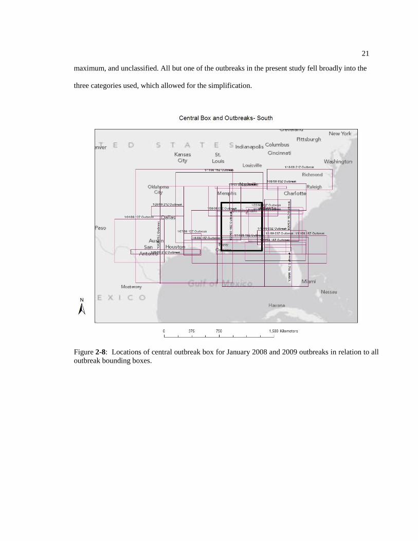
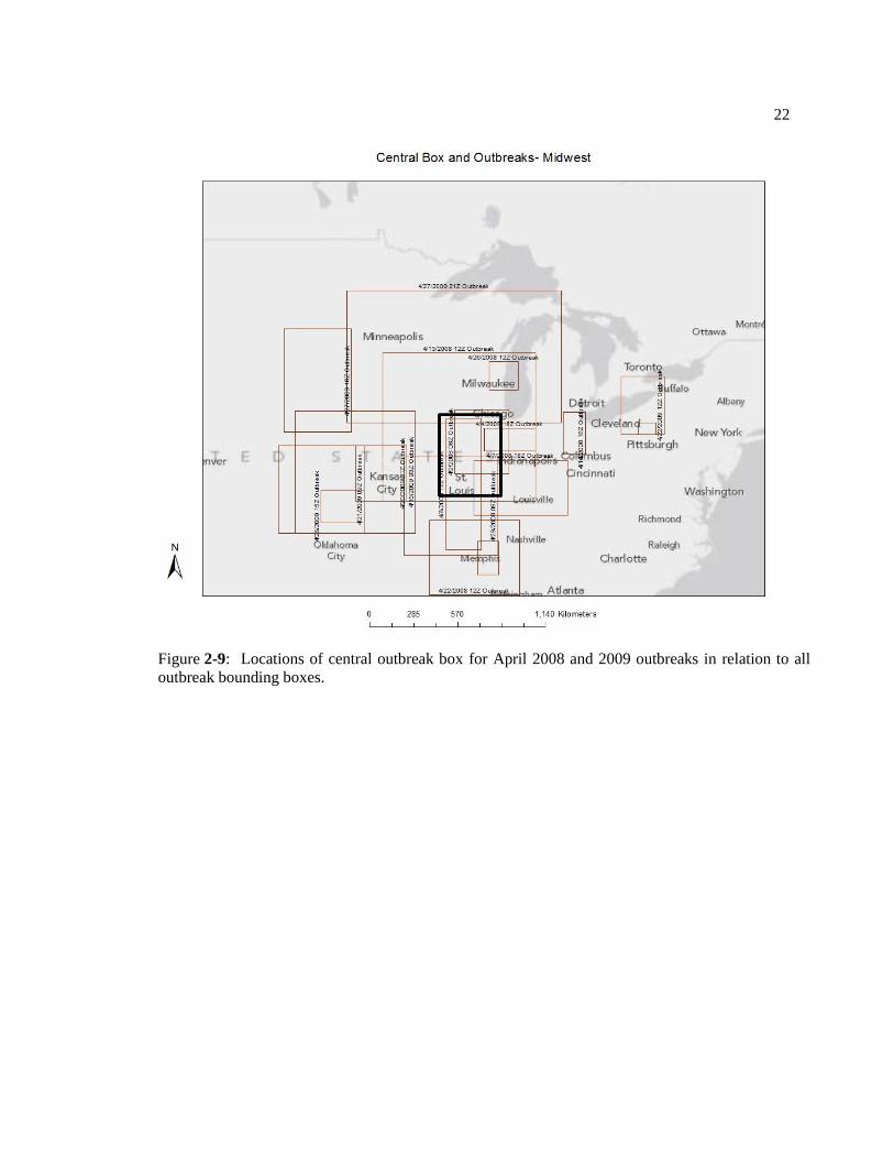
the majority of the outbreaks covered part or all of the central grid box. Figures 2-8 and 2-9 show

the location of the two central grid boxes used for the 250 mb composites, in relation to all of the

outbreaks (Figures 2-6 and 2-7). The representative grid box for each month and region was in a

fixed location, at the average location of the all of the region’s outbreaks, as determined by the

ArcGIS centroid tool. The size of the box was established as the average size of all the outbreak

bounding boxes. Lastly, to determine the synoptic circulation category associated with each

outbreak, the 500 mb height pattern present over each outbreak was determined from the NARR

data, and each outbreak was categorized as being inside a trough axis, between a trough and

ridge, or in a flat wave. These three categories are a simplified version of the categorization done

by DeGrand et al. (2000, Figure 11a.) for outbreaks, which included six additional categories-

closed low, closed high, at or near ridge axis, zonal flow with a weak height gradient, jet stream

21

maximum, and unclassified. All but one of the outbreaks in the present study fell broadly into the

three categories used, which allowed for the simplification.

Figure 2-8: Locations of central outbreak box for January 2008 and 2009 outbreaks in relation to all

outbreak bounding boxes.

22

Figure 2-9: Locations of central outbreak box for April 2008 and 2009 outbreaks in relation to all

outbreak bounding boxes.

Chapter 3

DTR Impacts of Longer-Lived Jet Contrail Outbreaks

In both regions and mid-season months, the longer-lived contrail outbreaks suppressed

DTR at the outbreak station versus at the adjacent non-outbreak station (Tables 3-1, 3-2). This

reduction in DTR underneath outbreaks is statistically significant at greater than the 95% level for

each studied month and region, although the outbreaks in the South during January had an even

stronger impact on the DTR. For those 24 outbreaks, DTR averaged 6.417 oF smaller than at the

nearby non-outbreak stations. For the 18 Midwest April outbreaks, the DTR was suppressed an

average of 5.278 oF. Although most outbreaks reduced DTR at the outbreak station, this was not

always the case (Table 3-1). In four of the January outbreaks (South) and three of the April

outbreaks (Midwest), DTR was either the same or slightly greater at the station affected by the

contrail outbreak. It is possible that these cases were a result of microclimatological or

observational biases in the stations used that could not be accounted for in the station selection

process. It is even more likely that the DTR suppression caused by each outbreak varies

considerably, with maximum suppressions of 27 oF (during April) and 25

oF (during January).

To further evaluate the DTR suppression of the contrail outbreaks, DTR at each

“adjacent” station (outbreak, non-outbreak) pair was normalized by comparing the observed DTR

for the outbreak to the long-term station average DTR for that date. These results also indicate

that the contrail outbreaks reduced DTR and that their impact on DTR outweighed the impact of

the larger-scale synoptic pattern on DTR. This effect was again most apparent during the January

South outbreaks, with the non-outbreak stations having a DTR of 2.833 oF above normal, and the

outbreak stations having a DTR of 2.708 oF below normal. For the April Midwest outbreaks, the

non-outbreak stations had a DTR of 2.722 oF above normal, while the outbreak stations had a

24

DTR of 1.611 oF below normal. Table 3-2 shows the composite DTR differences for each set of

outbreaks. To further distinguish the DTR impact of the contrail outbreak from other possible

influences, the DTR at each station for the day before and after the outbreak was determined

(Table 3-3). For each set of outbreak events, the average DTR difference between the outbreak

and non-outbreak stations was considerably smaller on both the day before and the day after the

outbreak. For the January South outbreaks, the DTR was only suppressed by 1.25 oF at the

outbreak stations on the day before or after the actual outbreak, compared to the non-outbreak

station. Moreover, for the April Midwest outbreaks, the DTR was only reduced by 2.639 oF at the

outbreak versus non-outbreak stations on the day before and after the actual outbreak. Unlike the

contrail outbreak days, neither the DTR suppressions during the day before and the day after the

outbreak were statistically significant, nor was there a statistically significant difference between

the DTR reduction of the day before or the day after the outbreak.

Table 3-1: DTR impacts of longer-lived jet contrail outbreaks.

Outbreak

Date/Time

Outbreak

DTR

Non-

Outbreak

DTR

DTR

Difference

Outbreak

DTR

Anomaly

Non-

Outbreak

DTR

Anomaly

January (South)

15z 1/3/2008 18 17 1 1 -1

12z 1/4/2008 27 29 -2 3 6

12z 1/7/2008 12 20 -8 -7 -3

18z 1/7/2008 11 21 -10 -10 1

3z 1/8/2008 11 27 -16 -8 10

3z 1/8/2008 19 26 -7 -1 4

15z 1/11/2008 16 23 -7 -1 4

18z 1/14/2008 20 27 -7 -4 2

12z 1/15/2008 22 23 -1 -1 4

21z 1/18/2008 11 16 -5 -8 -2

03z 1/22/2008 8 18 -10 -11 -7

18z 1/23/2008 10 35 -25 -13 8

25

3z 1/26/2008 9 6 3 -10 -10

18z 1/29/2008 28 29 -1 8 7

15z 1/30/2008 22 29 -7 0 6

03z 1/1/2009 18 32 -14 -6 8

15Z 1/1/2009 23 25 -2 3 7

03Z 1/5/2009 10 8 2 -8 -12

15Z 1/8/2009 20 20 0 0 0

03Z 1/11/2009 19 26 -7 -3 2

18Z 1/11/2009 19 26 -7 -3 2

03Z 1/18/2009 37 40 -3 15 18

21Z 1/26/2009 17 22 -5 -5 1

21Z 1/28/2009 23 39 -16 4 13

April (Midwest)

06z 04/02/2008 18 24 -6 -4 4

12z 04/06/2008 25 26 -1 2 3

18z 04/07/2008 31 32 -1 8 9

12z 04/13/2008 6 33 -27 -18 9

18z 04/14/2008 22 25 -3 2 1

12z 04/22/2008 20 23 -3 -2 1

12z 04/25/2008 20 26 -6 -3 2

12z 04/26/2008 18 21 -3 -1 1

18z 04/27/2008 16 26 -10 -8 2

09z 04/29/2008 17 26 -9 -4 1

03z 04/02/2009 27 30 -3 9 13

18z 04/04/2009 26 26 0 5 5

03z 04/15/2009 27 27 0 5 4

21z 04/20/2009 21 23 -2 -3 -2

09z 04/21/2009 24 29 -5 0 4

12z 04/22/2009 10 21 -11 -8 -1

15z 04/26/2009 19 25 -6 -4 -1

21z 04/27/2009 20 19 1 -5 -6

26

Table 3-2: Composite DTR impacts of jet contrail outbreaks.

Outbreak

Month, Region

Outbreak

DTR

Non-

Outbreak

DTR

DTR

Difference

Outbreak DTR

Anomaly

Non-

Outbreak DTR

Anomaly

Janaury, South 17.917 24.333 -6.417 -2.708 2.833

April, Midwest 20.389 25.667 -5.278 -1.611 2.722

Table 3-3: Composite DTR Impacts of days before and after jet contrail outbreaks.

Outbreak

Month, Region

Day Outbreak Non-Outbreak Outbreak DTR –

Non- Outbreak DTR

Janaury, South Day of

Outbreak

17.917 24.333 -6.417

Day before

and day after

22.458 23.708 -1.25

April, Midwest Day of

Outbreak

20.389 25.667 -5.278

Day before

and day after

20.694 23.333 -2.639

27

Chapter 4

Synoptic Climatology of Longer-Lived Jet Contrail Outbreaks

Two sub-regional synoptic climatologies (composites of synoptic environmental

conditions) of longer-lived contrail outbreaks were developed, one for the 24 outbreaks in the

South during January 2008 and 2009, and the other for the 18 outbreaks in the Midwest during

April 2008 and 2009. The two climatologies reveal key similarities and differences amongst the

several atmospheric variables analyzed.

The South January 2008 and 2009 Jet Contrail Outbreaks

The composite maps for the 24 January South outbreaks show internally consistent

patterns among all of the outbreaks. Throughout the representative grid box, there were

anomalously low temperatures at 250 mb – about -49 and -52 oC, or 0.4 to 1.6

oC below the 32-

year normal (Figures 4-1, 4-2). Moreover, the composite 250 mb zonal winds showed the

southern edge of a jet streak, with wind speeds of 43 to 46 ms-1

in the northwestern area of the

representative grid box. These winds were 4 to 6 ms-1

faster than normal. The rest of the grid box

outside the jet streak had zonal winds near or below normal (Figures 4-3, 4-4), thereby giving an

enhanced horizontal anomaly gradient. Finally, the 250 mb specific humidity was near normal

over the entire grid box (Figure 4-5).

Numerically, the UT variables also showed only slight deviations from normal across the

outbreak grid boxes. At 300 mb, the grid box-average specific humidity for the 24 outbreaks was

about 25% lower than normal; 1.647 x 10-4

g kg-1

, as opposed to the normal value of 2.194 x 10-4

g kg-1

. Moreover, the grid-box average 300 mb temperatures and zonal winds were both near

normal. Average 300 mb temperature was -42.937 oC (0.265

oC above normal) while 300 mb

zonal wind was 36.873ms-1

(1.4 ms-1

above normal). At 200 mb, the temperature showed a

28

slightly positive anomaly from normal, with a composite gridbox average of 59.240 oC (1.534

oC

below normal). These results suggest that there need not be anomalous UT conditions for the

formation of long-lived contrail outbreaks; however, temperatures below -40 oC at the contrail

formation level were a necessary condition.

Although the average (as well as maximum and minimum) values of the atmospheric

variables in the grid boxes were not significantly different from normal when all outbreaks were

composited, some of the associated horizontal gradients across the grid boxes were significantly

enhanced (Table 4-1). In particular, anomalously large horizontal gradients of 300 mb specific

humidity, 300 mb zonal wind, and 200 mb temperature were several times larger than normal and

statistically significant at the 95% level. The composite average grid-box minimum value of those

three UT variables was always below normal during long-lived outbreaks, while the composite

average maximum was always above normal, leading to the larger than normal gradients. Figure

4-6 shows an example of such a large gradient for a particular outbreak (1/08/2009), in this case

in the 200 mb temperature field. The bolded square shows the outbreak bounding box, which is

over half-covered by a zone of very tight temperature gradient, from relatively warm in the north-

eastern area of the box to cold in the western area.

Enhanced vertical gradients of the UT variables were also present in the outbreak station

composites. At the 300 mb level over the outbreak station, the average temperature was slightly

above normal, while the average temperature at 200 mb was below normal. This difference

resulted in a composite temperature change between 300 and 200 mb of 16.22 oC, a 2.52

oC larger

difference than normal (Table 4-2). A visual comparison of the composite outbreak station

vertical temperature profile with the normal profile confirms this large gradient in the UT, as

temperature transitioned from above average below the UT to below normal in and above it

(Figure 4-7). Figure 4-8 shows the departure from normal of the temperature profile, highlighting

29

the warmer than average lower and middle tropospheric levels, the colder than normal UT, and

the shift between these two zones at around 300 mb for the outbreak stations.

Vertical patterns in zonal winds commensurate with the temperature profiles were also

present over the outbreak stations. At and near the surface, zonal wind speeds were relatively

weak and below normal, suggesting high pressure. Between about 900 and 300 mb, though, zonal

winds were greater than normal and consistent with the temperature profile, but they switched

back to below normal just above the 300 mb level (Figure 4-9, 4-10). Directional shear in the UT

over the outbreak stations also exhibited an anomalous pattern comparable to the long-term

normals. The composite absolute directional shear between 300 and 100 mb for the outbreaks was

6.27 degrees, well above the climatological normal of 0.90 degrees. Fourteen of the 24 outbreaks

had associated clockwise turning of the wind through the UT (i.e., warm air advection), while 10

of the outbreaks had counter-clockwise turning of the wind (cold air advection).

There were three distinct types of larger-scale 500 mb patterns – which follow the

classification scheme found in De Grand et al. (2000) – present during the 24 outbreaks. Eighteen

of the outbreaks occurred between a trough and ridge axis, of which 12 were east of the trough

and 6 were east of the ridge. The remaining 6 outbreaks were in a trough axis. Table 4-3 classifies

each outbreak into its 500 mb and shear category, and also contains their numerical horizontal

gradients anomalies of specific humidity (at 300 mb) and temperature (at 200 and 300 mb).

Notably, the horizontal gradients of 300 mb specific humidity and 200 mb temperature were each

greater than normal for all but one of the outbreaks.

30

Figure 4-1: 250 mb temperature composite for January South region outbreaks.

Figure 4-2: 250 mb temperature composite anomaly for January South region outbreaks.

31

Figure 4-3: 250 mb zonal wind composite for January South region outbreaks.

Figure 4-4: 250 mb zonal wind composite anomaly for January South region outbreaks.

32

Figure 4-5: 250 mb specific humidity composite anomaly for January South region outbreaks.

Table 4-1: Composite horizontal gradients of UT variables for January South region

outbreaks. The ‘X normal’ denotes how many times greater than normal the gradient for

the composite of the selected outbreaks was.

300 mb SH 300 mb Temp 300 mb U Wind 200 mb Temp

Gradient

(/km)

Gradient

(C/km)

Gradient (m/s/km) Gradient

(C/km)

Outbreak 1.304E-07 0.0034 0.0206 0.0053

Normal 4.680E-08 0.0031 0.0056 0.0007

Anomaly 8.364E-08 0.0002 0.0150 0.0045

X normal 2.787 1.071 3.660 7.137

33

Figure 4-6: Sample 200 mb temperature gradient for 1/8/09 outbreak.

Table 4-2: Composite station UT data for January South region outbreaks.

Gradients Outbreak Normal Anomaly Standardized

Anomaly

300 mb T -57.204 -55.307 -1.897 -0.483

200 mb T -41.256 -41.605 0.346 0.103

300 mb SH 1.52E-6 1.42E-6 9.69E-06 0.129

300 mb U 34.607 34.188 0.419 0.014

Lapse rate Outbreak Normal Anomaly

300 - 200 mb T 16.219 13.695 2.524

34

Figure 4-7: Composite vertical temperature profile for January South outbreaks.

Figure 4-8: Composite vertical temperature anomalies for January South outbreaks.

35

Figure 4-9: Composite vertical zonal wind profile for January South outbreaks.

Figure 4-10: Composite vertical zonal wind anomalies for January South outbreaks.

36

Table 4-3: Synoptic Analysis of January South outbreaks.

Date CIRCUL Δ

|SHEAR|

S (C,

W)

ΔT-grad,

300 mb

ΔT-grad,

200 mb

ΔSH-grad Area

1/3/2008 East of

Ridge

3.16 W 4.40E-04 2.40E-03 4.13E-05 7.58E+05

1/4/2008 East of

Trough

-1.74 W 8.03E-04 4.65E-03 3.78E-05 2.55E+05

1/7/2008 East of

Trough

0.61 C 2.76E-05 4.67E-03 1.64E-05 5.18E+04

1/7/2008 East of

Trough

3.36 W 1.90E-03 2.85E-03 3.22E-05 1.48E+06

1/8/2008 East of

Trough

0.38 C 1.95E-03 -1.67E-

03

6.05E-05 2.96E+05

1/8/2008 East of

Trough

8.70 W 5.58E-06 6.29E-03 3.42E-07 2.58E+05

1/11/2008 Trough

Axis

9.44 W 8.82E-04 2.40E-03 2.70E-05 7.93E+05

1/14/2008 Trough

Axis

3.50 C 2.57E-04 8.39E-03 8.65E-05 6.11E+05

1/15/2008 East of

Trough

2.95 W 1.20E-03 4.37E-03 1.69E-04 2.15E+05

1/18/2008 East of

Trough

10.23 W 2.98E-04 9.80E-03 1.20E-04 1.59E+05

1/22/2008 East of

Trough

-0.81 C 6.97E-04 4.38E-03 1.33E-05 5.06E+04

1/23/2008 East of

Trough

7.68 C -8.64E-

04

7.03E-04 6.83E-05 1.60E+05

1/26/2008 East of

Ridge

6.22 W 1.56E-03 8.32E-03 1.17E-05 1.77E+04

1/29/2008 East of

Ridge

2.82 W -1.87E-

03

3.40E-03 5.70E-05 1.82E+05

1/30/2008 Trough

Axis

14.58 W -2.97E-

03

4.07E-03 1.19E-04 1.52E+05

1/1/2009 East of

Ridge

2.78 W 1.31E-03 1.71E-03 5.52E-05 5.34E+05

1/1/2009 East of

Ridge

-0.74 W 6.31E-04 3.19E-03 4.53E-05 5.00E+05

1/5/2009 East of

Trough

4.8 C 4.10E-03 2.46E-04 2.02E-04 2.60E+05

1/8/2009 Trough

Axis

21.43 C -3.04E-

03

1.86E-02 9.00E-05 3.99E+05

1/11/2009 East of

Trough

0.62 W -1.00E-

03

2.59E-03 8.96E-05 6.41E+04

1/11/2009 Trough

Axis

1.13 C 6.49E-06 4.19E-03 2.51E-04 1.50E+05

1/18/2009 East of

Trough

16.84 W -1.23E-

03

4.98E-03 1.63E-04 4.03E+04

37

The Midwest April 2008 and 2009 Jet Contrail Outbreaks

The composite maps for the representative grid box maps covering the 18 Midwest

region April outbreaks demonstrated internally consistent patterns, with near normal conditions.

The 250 mb temperature increased from west to east across the grid box, ranging from

approximately -51.7 to -52.7 oC (Figure 4-11). This resulted in negative temperature anomalies of

up to 0.6 oC in the southern and western portions of the grid box, and positive temperature

anomalies of up to 0.4 oC in the northern and eastern portions (Figure 4-12). The 250 mb zonal

wind composite map indicates above-normal westerly wind speed (up to 3 ms-1

) over nearly the

entire grid box (Figure 4-13). Zonal winds averaged 24 to 28 ms-1

, with a jet streak apparent in

the southern and western portions of the grid box (Figure 4-14). Additionally, both 250 mb

specific humidity values and their anomalies were rather variable throughout the grid box (Figure

1/26/2009 East of

Ridge

-0.19 C -1.68E-

04

2.64E-03 1.16E-04 5.61E+03

1/28/2009 Trough

Axis

11.09 C -5.33E-

04

6.60E-04 -8.72E-06 4.60E+04

Average: 6 East of

Ridge

5.37* 14 W 1.83E-04 4.33E-

03*

8.10E-05* 3.10E+05

12 East

of

Trough

10 C

6 Trough

Axis

Table 4-3 Note: Synoptic analysis of 24 contrail outbreaks analyzed in January 2008 and January

2009. Circulation categories (CIRCUL) at 500 hPa follow DeGrand et al. (2000). Both the

departure of the absolute value of vertical shear from the long-term normal (Δ |SHEAR| = S, m/s),

and the sign of the temperature advection (S, C = Cold, W= Warm) pertain to the layer 300-100

hPa. Departures of the horizontal gradients of temperature (ΔT-grad, in oC/km) and specific

humidity (ΔSH-grad, in g/kg/km) from the long-term normals at 300 hPa (and 200 hPa for

temperature) are calculated across the extent of each outbreak. Asterisks (*) indicate statistical

significance at p < 0.05 level.

38

4-15), suggesting that specific humidity was not a key UT variable controlling contrail outbreak

formation.

Small UT anomalies were also present in the composite numerical outbreak grid box

averages for the April outbreaks. The average 300 mb temperature was -45.614 oC (0.835

oC

below normal). The average 200 mb temperature, however, was -55.479 oC (1.292

oC above

normal), meaning a smaller than normal temperature lapse rate was occurring in the UT. The

average 300 mb zonal wind was 21.845 ms-1

; 0.584 ms-1

below normal, and 300 mb specific

humidity was 12% lower than normal- indicating that large anomalies in these UT variables were

not necessary for longer-lived outbreaks.

Large horizontal gradients of the UT variables occurred across the 18 outbreak grid boxes

(Table 4-4). Notably, the gradients of 200 mb temperature, 300 mb zonal wind, and 300 mb

specific humidity, were all several times larger than normal and statistically significant at the

95% level. They resulted from grid box-maximum values of each variable being higher than

normal, and grid box-minimum values being lower than normal.

An anomalous pattern in the vertical temperature profile emerged for the composite of

the outbreak station conditions (Figure 4-16). Between the surface and 300 mb, temperature was

consistently 1 to 2 oC below normal over the outbreak stations (Figure 4-17). However, above

300 mb, the temperature decreased at a much smaller rate than normal, and formed an inversion

located at around 175 mb, where the temperature peaked at 2 oC above normal. This vertical

temperature pattern for outbreaks also resulted in a smaller than normal lapse rate between 300

mb and 200 mb over the 18 Midwest stations (Table 4-5).

The vertical zonal wind profiles over the outbreak stations showed a consistent signature

with the temperature. Zonal winds were stronger than average between the surface and 300 mb,

peaking at nearly 3.5 ms-1

above normal at 500 mb (Figure 4-18, 4-19). Above 300 mb, though,

winds speeds were below normal. Normally, zonal winds peak at about 26 ms-1

at the 200 mb

39

level; however, for the outbreak station composite, zonal winds peaked at just 24 ms-1

.

Noteworthy is that the directional shear occurred over the outbreak stations: the average absolute

wind shear between 300 and 100 mb was 16.53 degrees, 15.10 degrees greater than the

climatological normal of 1.43 degrees. Three outbreaks in particular had exceptionally large wind

shear values of at least 40 degrees. Eleven outbreaks had counter-clockwise turning (cold air

advection), while 7 had clockwise turning (warm air advection), and one outbreak had no

directional wind shear. This result indicates that there is a range of advection conditions

associated with Midwest April outbreaks.

Similar to the January South region outbreaks, there were three different types of larger-

scale 500 mb patterns present during the 18 Midwest April outbreaks. Eleven of the outbreaks

were between a trough and ridge axis, of which 6 were east of the trough and 5 were east of the

ridge. The remaining 6 outbreaks took place in a trough axis, while one was situated in a zonal

weak gradient flow (as defined by DeGrand et al. 2000). Table 4-6 classifies each outbreak into

its 500 mb and shear category and also contains their numerical horizontal gradients of specific

humidity and temperature. Notably, the horizontal gradients of 300 mb specific humidity and 200

mb temperature, as well as shear between 300 and 100 mb, were each larger than normal for all

but one of the outbreaks.

40

Figure 4-11: 250 mb temperature composite for April Midwest region outbreaks.

Figure 4-12: 250 mb temperature composite anomaly for April Midwest region outbreaks.

41

Figure 4-13: 250 mb zonal wind composite for April Midwest region outbreaks.

Figure 4-14: 250 mb zonal wind composite anomaly for April Midwest region outbreaks.

42

Figure 4-15: 250 mb specific humidity composite anomaly for April Midwest region outbreaks.

Table 4-4: Composite horizontal gradients of UT variables for April Midwest region outbreaks.

The ‘X normal’ denotes how many times greater than normal the gradient for the composite of

the selected outbreaks was.

300 mb SH 300 mb Temp 300 mb U Wind 200 mb Temp

Gradient (/km) Gradient

(C/km)

Gradient (m/s/km) Gradient

(C/km)

Outbreak 1.342E-07 0.0056 0.0224 0.0075

Normal 2.775E-08 0.0033 0.0051 0.0012

Anomaly 1.068E-07 0.0023 0.0173 0.0063

X normal 4.837 1.691 4.413 6.350

43

Table 4-5: Composite station UT data for April Midwest region outbreaks.

Gradients Outbreak Normal Anomaly Standardized

Anomaly

300 mb T -57.204 -55.307 -1.897 -0.483

200 mb T -41.256 -41.605 0.346 0.103

300 mb SH 1.52E-6 1.42E-6 9.69E-06 0.129

300 mb U 34.606 34.188 0.419 0.014

Lapse rate Outbreak Normal Anomaly

300 - 200 mb T 16.219 13.695 2.524

Figure 4-16: Composite vertical temperature profile for April Midwest outbreaks.

44

Figure 4-17: Composite vertical temperature anomalies for April Midwest outbreaks.

Figure 4-18: Composite vertical zonal wind profile for April Midwest outbreaks.

45

Figure 4-19: Composite vertical zonal wind anomalies for April Midwest outbreaks.

Table 4-6: Synoptic Analysis of April Midwest outbreaks.

Date CIRCUL Δ

|SHEAR|

S (C,

W)

ΔT-grad,

300 mb

ΔT-grad,

200 mb

ΔSH-

grad

Area

4/2/2008 Flat

Wave

3.60 Cold 3.77E-03 2.26E-03 6.35E-08 8.46E+04

4/6/2008 East of

Trough

4.93 Warm -3.41E-

04

-1.69E-

04

2.53E-08 1.19E+05

4/7/2008 East of

Trough

5.36 Warm 6.36E-03 5.63E-03 5.13E-08 1.32E+05

4/13/2008 Trough

Axis

9.83 Cold 1.02E-03 5.88E-03 3.88E-10 5.36E+05

4/14/2008 Trough

Axis

9.90 Cold 8.49E-03 1.04E-03 7.71E-08 2.20E+04

4/22/2008 East of

Ridge

4.39 Cold -3.08E-

04

4.62E-03 1.01E-07 1.87E+05

4/25/2008 East of

Trough

21.17 Warm -6.33E-

04

5.83E-03 7.19E-08 1.92E+04

4/26/2008 Trough

Axis

2.00 Warm 4.32E-03 1.70E-02 8.61E-08 1.83E+04

46

Comparison of the January South and April Midwest Outbreak UT Conditions

The two months and regions analyzed in this study were not entirely similar in terms of

the synoptic patterns associated with outbreaks, although some important similarities exist.

Specifically, large horizontal gradients in the UT variables and strong wind shear were present for

both mid season months and regions, while specific humidity was typically below normal in the

4/27/2008 Trough

Axis

73.23 Cold 4.46E-03 1.12E-02 5.25E-09 1.54E+05

4/29/2008 East of

Ridge

35.67 Cold 1.32E-03 5.50E-03 2.25E-08 2.44E+05

4/2/2009 East of

Trough

16.32 Cold 1.00E-05 2.55E-03 -5.00E-

10

4.66E+03

4/4/2009 East of

Ridge

3.40 Warm 8.78E-04 2.55E-03 4.54E-08 2.82E+04

4/15/2009 East of

Ridge

16.69 Cold 1.74E-03 6.28E-03 1.55E-07 3.69E+05

4/20/2009 Trough

Axis

46.01 Cold 2.01E-03 2.20E-03 1.00E-07 7.20E+04

4/21/2009 East of

Ridge

40.40 Cold -1.01E-

04

1.93E-02 6.23E-08 1.94E+05

4/22/2009 Trough

Axis

0.00 NONE 1.03E-03 1.12E-02 4.60E-08 5.73E+04

4/26/2009 East of

Trough

0.82 Warm -2.33E-

03

4.99E-04 7.64E-07 3.67E+04

4/27/2009 East of

Trough

3.76 Cold 9.28E-03 6.97E-03 2.40E-07 6.10E+05

Average: 1 Flat

Wave

16.53* 11 C 2.28E-03 5.77E-

03*

1.06E-

07*

1.60E+05

6 Trough

Axis

6 W

6 East of

Trough

5 East of

Ridge

Note: Synoptic analysis of 18 contrail outbreaks analyzed in April 2008 and April 2009.

Circulation categories (CIRCUL) at 500 hPa follow DeGrand et al. (2000). Both the departure of

the absolute value of vertical shear from the long-term normal (Δ |SHEAR| = S, m/s) and the sign

of the temperature advection (S, C = Cold, W= Warm) pertain to the layer 300-100 hPa.

Departures of the horizontal gradients of temperature (ΔT-grad, in oC/km) and specific humidity

(ΔSH-grad, in g/kg/km) from the long-term normals at 300 hPa (and 200 hPa for temperature) are

calculated across the extent of each outbreak. Asterisks (*) indicate statistical significance at p <

0.05 level.

47

UT. Furthermore, neither set of outbreaks occurred during times of statistically significant

departures from normal of the UT variables in the representative and outbreak grid boxes,

although their horizontal gradients of the UT variables were significantly larger than normal. The

outbreaks in each region generally took place during the same time of day, primarily during the

daylight or late evening hours, when air traffic typically peaks.

The two sets of outbreaks varied substantially when considering the larger-scale synoptic

patterns present at 500 mb. Twelve of the 24 January South outbreaks occurred east of a trough,

while 14 of the 24 had associated warm advection occuring in the UT (Table 4-3). However, the

April Midwest outbreaks were almost evenly split bewteen the three circulation categories (east

of trough, east of ridge, in trough axis), and also had a majority of outbreaks occuring with cold

advection present in the UT. The April outbreaks generally had a warmer than normal UT,

especially at and above 250 mb, as the occurrence of cold advection did not necessarily preclude

a warmer than normal UT. Conversly, the January South outbreaks had an anomalously cold UT

above 300 mb, whereas the lower and mid levels of the atmosphere were warmer than normal for

the January outbreaks, but colder than normal for the April Midwest outbreaks. These differences

also were manifest in the vertical temperature profiles over the outbreak stations and in the

composite outbreak grid box data. In particular, the vertical temperature profiles (throughout the

entire troposphere) show stark differences, especially in the UT, as a slight inversion around 200

mb was present over the composite of the April Midwest outbreaks, while a larger than normal

decrease in temperature occurred in the composite of the January outbreaks. These differences

indicate that there was not one particular synoptic setup (e.g., in a trough or ridge axis) which

favored the formation of longer-lived contrails.

The zonal wind patterns also showed some differences between the two sets of regional

and mid-season month outbreaks. Climatologically, the South region outbreaks occurred with a

stronger westerly jet stream, as the long-term normal zonal winds peaked at around 42 ms-1

at 200

48

mb, while those in the Midwest outbreaks peaked at only 27 ms-1

. Each of the outbreaks had

weaker than normal jets, with negative anomalies in the UT above 300 mb, although the

anomalies were twice as large in the Midwest outbreaks versus those in the South. Moreover,

zonal winds were stronger than normal below 300 mb for both sets of outbreaks, although for the

South region between 900 mb and the surface, zonal winds were weaker than normal.

Last, the January South region outbreaks, on average, covered a greater area than the

April Midwest outbreaks. The average Midwest outbreak grid box had an area of approximately

160,000 km2, while the South region grid boxes were nearly twice as large on average; about

310,000 km2 (Tables 4-3, 4-6). The outbreak grid boxes for each month and region also had

different orientations. Nine of the 18 April Midwest outbreak grid boxes were oriented north-to-

south (i.e., rectangular), with 6 being west-to-east, and 3 were square. Of the January South grid

boxes, though, 16 were oriented north-to-south, 4 were west-to-east, and 4 were square.These

results indicate that the area of contrail clouds did not need to be oriented in a particular direction

(e.g., north-to-south or east-to-west) to persist and create outbreaks.

49

Chapter 5

Summary, Discussion, and Conclusions

This chapter first discusses the results presented in Chapter 4 and suggests physical

explanations for them. Then, to motivate future work on the topic of contrail outbreaks and

climate feedbacks, it places the results of this study in the context of the broader-scale dialogue

on human-climate interactions involving jet aviation.

The findings indicate that the presence of longer-lived jet contrail outbreaks suppresses

the DTR at the underlying surface stations. For each set of outbreaks (January South, April

Midwest), there was a statistically significant suppression of DTR at stations compared to nearby

stations not overlain by contrails. The fact that the DTR station differences were not statistically

significant on either the days before or after the outbreak further validates this conclusion. This

result confirms prior work and physical reasoning (e.g., Travis et al. 2004), as the additional

cloudiness from jet contrail outbreaks helps reduce surface shortwave radiation receipt during the

day, and enhance longwave energy back-radiation receipts at night, thereby lowering the daily

maximum temperature and raising the daily minimum temperature. Although the January South

outbreaks had a slightly greater absolute impact on the DTR (reducing DTR by 1.139 oF more),

this difference was not statistically significant. However, the type of synoptic pattern present in

conjunction with the outbreaks may have influenced DTR. Those outbreaks occurring with UT

cold advection suppressed surface DTR by 7.57 oF (when comparing outbreak to non-outbreak

stations), while outbreaks occurring with warm advection only reduced DTR by 3.90 oF.

Similarly, outbreaks occurring in a 500 mb trough axis suppressed surface DTR by 9.08 oF,

contrasted with just 4.62 oF for those outbreaks located between trough and ridge axes. A possible

explanation for these variations is that the cold advection and associated trough axis in the two

regions were generally more favorable for cloud formation and development, because cold air

50

over a warm surface leads to instability and vertical motion, so the jet contrails that formed

during these conditions were more extensive and longer-lasting, thus having a greater opportunity

to affect DTR.

This research also confirms and extends the suggestion that specific UT conditions

accompany most longer-lived jet contrail outbreaks – at least those outbreaks affecting DTR in

the two regions and mid-season months studied. In particular, anomalously large horizontal

gradients of UT temperature, specific humidity, and zonal wind, along with strong vertical shear

in the UT, appeared necessary for outbreaks to form and persist. Collectively, these conditions are

representative of baroclinic zones, which suggests that their presence may have been necessary

for contrail outbreaks to be sufficiently well developed to influence DTR. Baroclinic zones occur

near troughs and jet streaks, and the composite grid box maps of zonal wind for each set of

outbreaks (January South, April Midwest) confirmed that the typical outbreak occurred in the

vicinity of a 250 mb jet streak and in conjunction with a large horizontal gradient of zonal wind.

The large zonal wind gradient helps explain why the station composites showed below-normal

zonal winds in the UT, because the compositing process “averages out” the steep wind gradients

and therefore suggests below-normal winds. Moreover, some outbreaks occurred within the 500

mb trough axis, and all except one took place in an amplified wave pattern, either between the

trough and ridge or within the trough axis. The fact that the outbreaks within a trough axis and/or

with strong cold advection and wind shear had the greatest impact on DTR underscores the

importance of baroclinic zones for the formation of DTR-suppressing jet contrail outbreaks. As

baroclinicity can occur at most times of the year in the extratropics, and with a wide range of

conditions (e.g., the type of air mass present), it is understandable that the results did not show

outbreak-to-outbreak consistency in the general UT conditions (e.g., temperature, zonal wind,

specific humidity at a particular pressure level, as well as vertical temperature profile). Therefore,

it is reasonable to conclude, at least for the 42 jet contrail outbreaks studied for the South and

51

Midwest sub-regions of the U.S. in January 2008-09 and April 2008-09, that baroclinic zones

provide a favorable location for jet contrail outbreaks to form, persist, and be sufficient to

suppress surface DTR. This finding reinforces the importance of contrails to surface temperatures

in those regions underlain by high frequencies of jet aircraft.

There are potential societal impacts associated with a suppressed DTR. One likely

consequence is an extended growing season in regions of frequent jet flights. Higher minimum

temperatures suggest that, the first frost of the season would be delayed in contrail-prone areas,

while the last frost of the spring or late winter would happen earlier. Growing season is also likely

increasing due to other anthropogenic factors (Hayhoe et al. 2007), but separating the effect of

contrails from these other influences would be useful to decision-makers when detailing their

impacts. DTR changes would also result in changes to annual heating and cooling degree days, a

measure of how much energy is necessary given the departure of a day’s average temperature

from 65 degrees. Depending on both the timing of contrail events and interplays with local

microclimates, contrails could either increase or reduce energy demands for heat or air

conditioning. During the summer, contrails could reduce the maximum temperatures by a few

degrees, thereby reducing energy requirements. In contrast, at night, a contrail-induced increase

in minimum temperatures could result in a net increase in energy consumption. At other times,

the moderating effect of jet contrails could potentially have the opposite impact of reducing

energy use, e.g., if temperatures do not fall as low during cold winter nights, not as much

residential heat is necessary. Intentionally manipulating surface temperature – specifically

increasing minimum temperatures in northeastern U.S. cities on cold nights through cloud

seeding and the formation of jet contrails – has been proposed as an early form of geo-

engineering (Detwiler and Cho 1982; Detwiler and Pratt 1984).

A wide range of extensions and applications of this research are possible and especially

pertinent as air travel continues to increase. Additional regions and outbreak months should be

52

studied to determine if the conclusions drawn from this work are more generally applicable in

space and time. Moreover, shorter-lived outbreaks over the study regions should be analyzed to

compare with the results of the longer-lived outbreaks. In terms of applications, the findings of

this research and follow-up studies could contribute to real-time forecasting of contrail outbreaks

in the near future, as the specific conditions necessary for their formation and persistence are

better understood. Given that longer-lasting outbreaks significantly suppress DTR, their

prediction and observation should be factored into weather forecast models (e.g., MOS) to better

predict surface temperatures. Finally, a better understanding of the formation and climatic

impacts of jet contrail outbreaks could bolster policy recommendations that help to curb this

human influence on weather and climate by making air traffic and airplanes more efficient. For

example, strategies to be employed could include re-routing planes around areas of favorable UT

conditions for longer-lived outbreaks, or flying at lower altitudes when and where these

conditions occur (Williams and Noland 2005).

53

References

Appleman, H., 1953: The formation of exhaust condensation trails by jet aircraft. Bulletin of the

American Meteorological Society, 34, 14–20.

Carleton, A.M. and P.J. Lamb, 1986: Jet contrails and cirrus cloud: a feasibility study

employing high-resolution satellite imagery. Bulletin of the American Meteorological

Society, 67, 301-309.

Carleton, A.M., D.J. Travis, K. Master, and S. Vezhapparambu: 2008. Composite

atmospheric environments of jet contrail outbreaks for the United States. Journal of

Applied Meteorology and Climatology, 47, 641-667.

Carleton, A.M., A.D. Silva, M.S. Aghazarian, J. Bernhardt, D.J. Travis, and J. Allard:

2013. Mid-season climate diagnostics of jet contrail "outbreaks,” and implications for eastern

U.S. sky cover trends. Climate Research, in press.

DeGrand, J.Q., A.M. Carleton, D.J. Travis, and P.J. Lamb, 2000: A Satellite-Based

Climatic description of jet aircraft contrails and associations with atmospheric

conditions, 1977-79. Journal of Applied Meteorology, 39, 1434-1459.

Detwiler A. and H. Cho, 1982: Reduction of residential heating and cooling requirements

possible through atmospheric seeding with ice-forming nuclei. Journal of Applied Meteorology,

21, 1045-1047.

54

Detwiler, A. and R. Pratt, 1984: Clear-air seeding: opportunities and strategies.

Journal of Weather Modification, 16, 46- 60.

Environmental Protection Agency Fact Sheet, 2000: Aircraft contrails factsheet. EPA430-F-00-

005.

Hanson, H.M. and D.M. Hanson, 1995: A reexamination of the formation of exhaust

condensation trails by Jet Aircraft. Journal of Applied Meteorology, 34, 2400-2405.

Hayhoe, K., and Coauthors, 2007: Past and future changes in climate and hydrological indicators

in the US Northeast. Climate Dynamics, 28, 381-407.

Forster, P., and Coauthors, 2007: Changes in atmospheric constituents and in radiative forcing.

Climate Change 2007: The Physical Science Basis. Contribution of Working Group I to the

Fourth Assessment Report of the Intergovernmental Panel on Climate Change [Solomon, S., D.

Qin, M. Manning, Z. Chen, M. Marquis, K.B. Averyt, M.Tignor and H.L. Miller (eds.)],

Cambridge, UK: Cambridge University Press.

Jensen, E. J., A. S. Ackerman, D. E. Stevens, O. B. Toon, and P.Minnis, 1998: Spreading and

growth of contrails in a sheared environment. Journal of Geophysical Research, 103, 31 557–31

567.

Karcher, B., U. Burkhardt, S. Unterstrasser, and P. Minnis, 2009: Factors controlling contrail

cirrus optical depth. Atmospheric Chemistry and Physics, 9, 6229-6254.

55

Lee, D. and Coauthors, 2009: Aviation and global climate change in the 21st century. Atmospheric

Environment, 43, 520-3537.

Mesinger, F., and Coauthors, 2006: North American regional reanalysis. Bulletin of the American

Meteorological Society, 87, 343–360.

Minnis, P., J.K. Ayers, and S.P. Weaver, 1997: Surface-based observations of contrail

occurrence frequency over the US, April 1993 – April 1994. NASA Reference

Publication 1404.

Minnis, P., J.K. Ayers, R. Palikonda, and D. Phan, 2004: Contrails, cirrus trends, and

climate. Journal of Climate, 17, 1671-1685.

National Weather Service. “What is a contrail and how does it form?”

Western Region Headquarters <http://www.wrh.noaa.gov/fgz/science/contrail.php>

Ryan, A. C., A. R. MacKenzie, S. Watkins, and R. Timmis, 2011: World War II contrails: A case

study of aviation-induced cloudiness. International Journal of Climatology, 31, 1745-1753.

Schrader, M. L., 1997: Calculations of aircraft contrail formation

critical temperatures. Journal of Applied Meteorology, 36, 1725–1728.

Silva, A.D., 2009: A composite-based retro-prediction method for jet contrail outbreaks over the

United States. M.S. thesis, Department of Geography, Pennsylvania State University, 159 pp.

56

Travis, D.J., A.M. Carleton, and S.A. Changnon, 1997: An empirical model to predict

widespread occurrences of contrails. Journal of Applied Meteorology, 36, 1211-1220.

Travis, D.J., A.M. Carleton, and R.G. Lauritsen, 2004: Regional variations in U.S.

diurnal temperature range for the 11-14 September 2001 aircraft groundings:

evidence of jet contrail influence on climate. Journal of Climate, 17, 1123-1134.

Travis, D.J., A.M. Carleton, J.S. Johnson, and J.Q. DeGrand, 2006: U.S. jet contrail

frequency changes: influences of jet aircraft flight activity and atmospheric conditions.

International Journal of Climatology, 27, 621-632.

Travis, D.J., A.S. Weberpal, and A.M. Carleton, 2011: Contrail impacts on diurnal temperature

range estimated from error analysis of meteorological model output statistics. Proceedings of the

56 Annual Meeting of the American Association of Geographers, April 2011.

Williams, V.and R.B. Noland, 2005: Variability of contrail formation conditions and the

implications for policies to reduce the climate impacts of aviation. Transportation Research Part

D: Transport and Environment, 10, 269-280.

Appendix A

Sample 500 mb Geopotential Height Maps

Figure A1: Contrail outbreak in trough axis. 12Z 4/13/2008 outbreak.

58

Figure A2: Contrail outbreak east of ridge. 18Z 4/4/2009 outbreak.

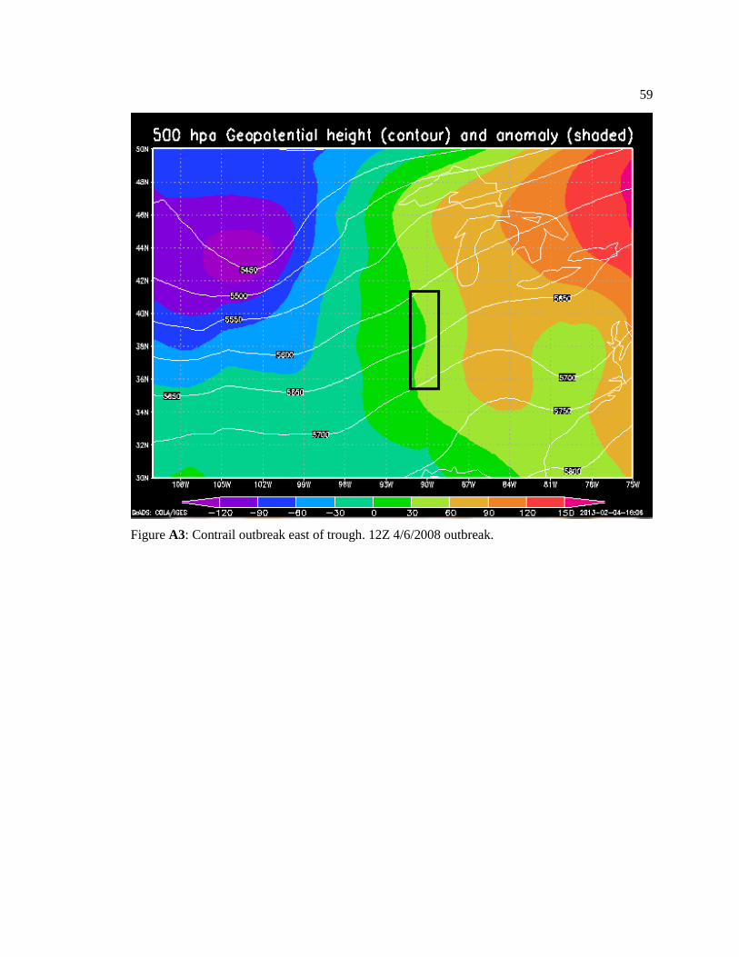
59

Figure A3: Contrail outbreak east of trough. 12Z 4/6/2008 outbreak.

60

Appendix B

Sample Upper Tropospheric Wind Shear Profiles

Figure B1: Sample of cold air advection over an outbreak. 18Z 4/27/2008 outbreak.

61

Figure B2: Sample of warm air advection over an outbreak. 15Z 1/30/2008 outbreak.