A Survey of The Impact of Operational Losses on ...
141
A SURVEY OF T1IK IMPACT OF OPERATIONAL LOSSES ON PROFITABILITY OF COMMERCIAL BANKS IN KENYA ONGERA JOSHUA BOSIRE D61/P/7631/02 SUPERVISOR: MRS. A. KITHINJI A MANAGEMENT RESEARCH PROJECT SUBMITTED IN PARTIAL FULFILMENT OF THE REQUIREMENT FOR THE AWARD OF THE DEGREE OF MASTER OF BUSINESS ADMINISTRATION SCHOOL OF BUSINESS UNIVERSITY OF NAIROBI SEPTEMBER 2006 Uravereity ol NAIROBI Library 0492950 1
Transcript of A Survey of The Impact of Operational Losses on ...

A SURVEY OF T1IK IMPACT OF OPERATIONAL LOSSES ON
PROFITABILITY OF COMMERCIAL BANKS IN KENYA
ONGERA JOSHUA BOSIRE
D61/P/7631/02
SUPERVISOR:
MRS. A. KITHINJI
A MANAGEMENT RESEARCH PROJECT SUBMITTED IN PARTIAL
FULFILMENT OF THE REQUIREMENT FOR THE AWARD OF THE DEGREE
OF MASTER OF BUSINESS ADMINISTRATION SCHOOL OF BUSINESS
UNIVERSITY OF NAIROBI
SEPTEMBER 2006
Uravereity ol NAIROBI Library
0492950 1

DECLARATION
This management research project is my original work and has not been presented
for the award of a degree in any other university.
Signed—
ONGERA JOSHUA BOSIRE
D61/P/7631/02
This management research project has been submitted for examination with my
approval as university supervisor.
mill/'oiANGELA KITHINJI (MRS)
Department of finance and accounting, school of business,
University of Nairobi
- 1 -

DEDICATION
This study is dedicated to my parents, brothers, sisters, nephews and
nieces without whose efforts and sacrifice I could not have progressed
this far. May their sacrifice and dreams of their hard work bear ripe
fruits.
AMEN.

ACKNOWLEDGEMENTS
I appreciate and wish to extend my gratitude to all those who in one- way or another
enabled me to complete this study. More especially:
• My supervisor Mrs. Kithinji; I thank her for her firm: decisive, timely and
invaluable advice and positive criticisms that were challenging and enabled me
focus on the objective of the study.
• My fellow colleagues at work Mr.Nzioki. Mr. Yussuf and Kenya Commercial
Bank library staff for sacrificing their valuable time to give me support
throughout my study.
• My friends for sacrificing their valuable time encouraging and supporting me
throughout my study.
• Last but not least to my parents, brothers, sisters, nephews and nieces without
w hose efforts and sacrifice I could not have progressed this far.
• M ay God bless you.
- in -

TABLE OF CONTENTS
PAGE
Declaration---------------------------------------------------------------------------------------------------i
Dedication--------------------------------------------------------------------------------------------------- ii
Acknowledgements--------------------------------------------------------------------------------------i i i
Table of Contents.............................................................................. iv
List of Abbreviations................................ vii
Abstract-------------------------------------------------------------------------------------------------- viii
CHAPTER ONE: INTRODUCTION---------------------------------- -------------------------- 1
1.1 Background----------------------------------- -------------------------------------------------------- 1
1.2 Statement o f the Problem......................................... ....................................... .................5
1.3 Objectives of the Study................................... -.............................................................. --6
1.4 Hypothesis........................................................................................................................... 6
1.5 Importance of the Study....................................................... -.................................-......... 6
CHAPTER TWO: LITERATURE REVIEW................................. ..................................9
2.1 Risk Management---------------------------------------- -------------------------- -.....................9
2.2 Operational Risk Management................................................................... ................... 10
2.3 Framework of Operational Risk Management.......................................... -...................12
2.4 Operational Losses...................... 24
2.5 Profitability.......... ................................................................................. 34
2.6 Related Studies..................................................... 36
CHAPTER THREE: RESEARCH METHODOLOGY-------------------------------------38
3.1 Research Design................................. 38
iv -

3.2 Population of Study.......................................................................................................... 38
3.3 Data Collection----------------------------------------------------------------------------------- 38
3.4 Data analysis------------------------------------------------ --------------------------------------- 38
CHAPTER FOUR: DATA ANALYSIS-------------------------------------------------------- 40
4.1.1 Industry Average........................................................................................................... 40
4.1.2 African Banking Corporation-------------------------------------------------------- 41
4.1.3 Bank o f Baroda---------------------------------------------------------------------------- 42
4.1.4 Barclays Bank of Kenya L td ................. 43
4.1.5 Commercial Bank o f Africa..........................................................................................44
4.1.6 CFC Bank Limited..................................................................................................... —45
4.1.7 Charterhouse Bank Limited....................................................................................... —46
4.1.8 Chase Bank Limited....................... ....................... -..................................................... 47
4.1.9 City Finance Bank------------------------------------------------------------------------------- 48
4.1.10 Consolidated Bank of Kenya......................................................................................... 49
4.1.11 Co-operative Bank of Kenya-------------------------------------- 50
4.1.12 Credit Bank Limited.................................. .................................................................. 51
4.1.13 Development Bank of Kenya.................................... 52
4.1.14 Diamond Trust Bank Kenya................................... 53
4.1.15 Equatorial Commercial B ank---------------------------------------------------------------- 54
4.1.16 Equity Bank Limited....................................................................................................55
4.1.17 Fina Bank Limited...................................... 56
4.1.18 First American Bank Limited..................................................................................... 57
4.1.19 Giro Commercial Bank.................................-..............................................................58
4.1.20 Guardian Bank---------------------------------------- -................................................—59
4.1.21 Habib Bank Limited.....................................................................................................60
4.1.22 Habib AG Zurich------------------------------------------------------------------------------- 61
4.1.23 Investment & Mortgages Bank...................................................................................-62
4.1.24 Imperial Bank Limited---------------------------------------------- ------------ -................ 63
2.1.25 Kenya Commercial Bank L td ..................................................................................... 64
- v -
4.1.26 Middle East Bank of Kenya------------------------------------------------------------------ 65
4.1.27 National Bank of Kenya Ltd....................................................................................... 66
4.1.28 Paramount-Universal B ank..........................................................................................67
4.1.29 Standard Chartered Bank Ltd.......................................................................................68
4.1.30 Stanbic Bank Kenya Limited----------------------------------------------------------------- 69
4.1.31 Transnational Bank Limited------------------------------------------------------------------ 70
CHAPTER FIVE: SUMMARY OF FINDINGS, CONCLUSIONS,
RECOMMENDATIONS, LIMITATIONS OF THE STUDY AND
SUGGETIONS FOR FURTHER RESEARCH --------------------------------------------- 71
5.1 Summary of Findings. Conclusions and Interpretations............................................... 71
5.2 Limitations of the Study------------------------------------------------------------------- 72
5.3 Recommendations---------------------------------------------------------- 73
5.4 Suggestions for Further Study.............................................................................. 73
REFERENCES-----------------------------------------------------------------------------------------75
APPENDICES------------------------------------------------------------------------------------------77
A 1.1 List o f Commercial Banks....................................................... 77
A 1.2 Table of Research Data...... ........................................................................................... 79
A 1.3 Table of Ratios.................................................................. 82
A1.4 Significance Tests------------------------------------------------------------------------ 86
- vi -

LIST OF ABBREVIATIONS
PAT/EBIT- Profit after tax (PAT) to Earnings before Interest and Tax (EBIT)
OP/EBIT- Operational losses to Earnings before Interest and Tax (EBIT)
OP/T OP EX- Operational losses to Total Operating Expenses
- V l l -

ABSTRACT
Profitability is cited as a major predictor or determinant of business failure. Ratios used
to measure profitability have shown to be suitable predictors of subsequent insolvency of
firms. This study addresses the impact of operational losses on profitability.
Data from 30 commercial banks was obtained and analyzed using SPSS package. This
study shows that there was an upward trend in year 2002, downward trend in 2003.
upward trend in 2004 and a dow nward trend in year 2005 of operational losses ratio for
the industry. This study shows a zigzag movement. The relationship between
profitability and level o f operational losses was found to be direct and negative for the
industry.
The findings reveal that the trend of operational loss level kept on varying from year to
year without a clear defined direction for most of the commercial banks. Most of the
commercial banks had an upward trend in years 2001, 2002 and 2003 followed by a
downward trend in years 2004 and 2005. The relationship between profitability and level
of operational losses was found to be direct and negative for most of the commercial
banks. Some commercial banks show a positive relationship such that increase in
operational losses will lead to increase in profitability. The relationship was found to be
significant. The category most affected is the big banks mostly government owned
commercial banks. The large foreign owned banks indicated lower significance levels as
compared to large locally owmed commercial banks. The small commercial banks foreign
owned indicated a lower significance level as compared to small locally owned
commercial banks.
The result o f this study is consistent with findings o f other researchers on the effect of
operational losses on profitability. This study shows that the impact of operational losses
on profitability of commercial banks is significant as opposed to general believe that the
impact of operational losses on profitability of commercial banks is not significant.
- viii -
CHAPTER ONE: INTRODUCTION
1.1 Background
1.1.1 Operational Losses Management
Banks like any other institutions play an important role in the economy. The auxiliary
services they offer to other institutions, corporate bodies and sectors o f the economy,
among others are numerous (Gruening and Bratanovic, 1999). Banks are sensitive
institutions in the economic environment, thus need for concern from all stakeholders in
the economy on their stability. They do act as intermediaries of funds between surplus
user units and deficit user units. For them to be able to play this role, their liquidity
position should be closely monitored. All banks are thus encouraged to have a risk-
management department whose sole responsibility is to report their liquidity position
regularly (Gruening and Bratanovic. 1999).
A service organization can encounter actual or speculative failure. The former might be
the failure o f a new service to deliver appropriate quality, speed, flexibility or expected
cost, and revenue performance. Whereas, speculative failure can be seen as the inability
to deploy operational or other resources where they can earn returns an idea similar to the
accountant's concept of an "opportunity cost''. Operational loss may generate a range of
negative consequences for an organization, for example, customer defection, damaged
corporate image, litigation and increased insurance costs (Brown et al. 2000; Dorner.
1997; Winter and Steger. 1998). The operations management and service management
literature often discusses loss control but failing to point out the impact of operational
loss on profitability (Schelesinger and Hesket. 1991; Chase and Stewart, 1994).
Operational loss includes items classified by banks as loan loss provision, depreciation,
amortization, and other operating expenses in the published financial statements (Basel
Committee 2000; Saunders 2000).
Good operational loss management is a decisive competitive advantage as it helps to
maintain stability and continuity and supports revenue and earnings growth in
commercial banks (Doering 2003). Risk management is an obligation to stakeholders
thus diligent and intelligent risk taking is an "attitude" towards stakeholders. Thus despite
all the progress in the quantification of operational losses, operational loss management
will remain a blend of art and science. Operational loss management is a daily struggle
against uncertainty and a daily learning process. Operational loss is part o f corporate life
particularly in financial institutions. Operational loss is highly multifaceted, complex and
often interlinked making it necessary to manage, rather than fear. While not avoidable,
operational loss is manageable - as a matter of fact most banks live reasonably well by
incurring operational losses, especially "intelligent operational losses", (Jorion, 2001).
Deregulation and globalisation of financial services, together with the growing
sophistication of financial technology, are making the activities of banks and thus their
risk profiles more complex. The Basel Committee on Banking and Supervision (2003)
suggests that risks other than credit, interest and market risks can be substantial.
According to Basel Committee (2003). the greater use of highly automated technology
has the potential to transform risks from manual processing errors to system failure risks
as greater reliance is placed on globally integrated systems. The growth o f e-commerce
brings with it potential risks such as internal and external frauds and systems security
issues that are not fully understood. The emergence of banks acting as large-volume
service providers creates the need for continual maintenance of high-grade internal
controls and backup systems. According to the Credit-Suisse Group (2001), banks may
engage in risk mitigation techniques to optimize exposure to market and credit risk but
which may in turn produce other forms of risk like operational risks which the group
categorized as organizational risks, process risks, technology risks, human risks and
external risks.
Commercial banks mainly engage on operating activities to generate revenue. These
activities in turn are the cause o f operational losses if not properly managed. Operational
losses have been defined, as the risk of loss resulting from inadequate or failed internal
. ? .

*
processes, people, and systems or from external events (Basel Committee 2000). The
Committee identified the following operational losses, which are likely to result into
substantial losses: internal frauds, which include intentional misreporting of positions,
employee theft, and insider trading on employee's own interest; external frauds through
robbery, forger), cheque kitting, and damage from computer hacking; employment
practices and work place safety relating to compensation claims, violation of employee
health and safety rules, organized labour activities, discrimination claims and general
liability; clients, products and business practices such as misuse of confidential customer
information, money laundering and sale of unauthorized products: damage to physical
assets through terrorism, vandalism, earthquakes, fires and floods; losses arising from
business disruptions and systems failures such as hardware and software failures,
telecommunication problems and utility outages; execution delivery and process
management, such as data entry errors, collateral management failures, incomplete legal
documentation, unapproved access given to client accounts and vendor disputes.
According to Dermont (2002) operational loss is not really one loss but many. It is a
sweep up term covering every thing that does not fall neatly under either credit loss or
market loss. One operational loss event can lead to another. Some financial events can
directly cause operational loss. The literature on operational loss and its management in
the service sector is overwhelmingly concerned with the suppression of negative
consequences of failure (Lewis, 2003). It does so by taking into consideration three
aspects of loss management, failure prevention, failure management and management via
recovery methods and insurance (Hollman and Forest. 1991). Some authors have
developed normative models of how decisions on long-term developmental issues can
accommodate learning from implementation of failure prevention and crises management
methods (Preeble. 1997). However there is little empirical research in the area of the
impact o f operational loss on profitability.
- 3 -
1.1.2 The Kenya Banking Sector
Commercial banking took root in Kenya at the turn of the 20lh century with the
partitioning o f Africa by the European imperial powers. The first bank to establish
operations was National Bark of India, which started a branch in Mombasa in 1896. By
1972. there were a total of .12 commercial banks operating in the Kenyan market. The
banking system currently has 44 commercial banks, 2 non- banking financial institutions,
2 mortgage finance companies and 3 building societies.
Weaknesses in the banking system became apparent in the late 1980s and were manifest
in the relatively controlled and fragmented financial system, differences in regulations
governing banking and non-bank financial intermediaries, lack of autonomy and weak
supervisory capacities to carry out its surveillance role and enforce banking regulations
by the Central Bank, inappropriate government policies which contributed to an
accumulation of non-performing loans, loss of control of money supply by the Central
Bank and non-compliance by financial institutions to regulatory requirements of the 1989
Banking Act among others.
In the earlier 1990s the government embarked on reforms designed to promote a more
efficient and market -oriented financial system, improve the mobilization, allocation and
utilization o f financial resources, increase the efficiency of the process of financial
intermediation, and develop more flexible instruments of monetary policy. The reform
program focused on policy, legal and institutional framework.
According to Basu and Rolfes (1995) deregulation dramatically change the operating
environment for banks. Since liberalization, the industry has undergone tremendous
changes. Competition resulted from micro-finance houses and Cooperative Societies,
which opened front-office operations providing serv ices very much similar to those of the
commercial banks and NBFIs converting to commercial banks (Koros, 2000). Because of
poor economic performance and dwindling good lending opportunities, banks have been
forced to diversify to non-balance sheet based income streams. Attracting this source of
- 4 -

income requires banks to take deliberate strategic initiatives towards improvement of the
product/service range and delivery channels (Market Intelligence. 2002).
1.2 Statement of the Problem
Given the important role that banks play in any economy, it is crucial to understand the
factors that influence their viability and survival. Instances of bank failure thus raise
important concerns to both local and foreign investors in any country. According to
Waciira (1999), the apparent variability of profitability of companies with time has real
implications for the business community, especially the banking sector. The recent
failures in banking industry have raised great concern and have forced banks to put more
emphasis on financial loss measures but this has not sorted out the problem of bank
failures.
Operating activities being the major dealings of commercial banks are one of the sources
of financial losses, which the banks incur. The dynamism of these activities creates
loopholes, which results to increased loan loss provision, depreciation, amortization, and
other operating expenses as published in the financial statements. Failure to effectively
manage operating activities results to operational losses emanating from both the internal
and external environment. Operating losses do impact on profits because it is charged to
the profit and loss account and they are merely cost additive. Proper control of the
operating loss directly translates to increased profits. Operational loss only appears when
it crystallizes in the form of an outflow and its potential is hidden thus need to discover
its impact on profits.
Yussuf (2005), conducted a study on management o f operational risk o f Commercial
Banks in Kenya and highlighted the need for a critical study on the impact of operational
losses on profitability of banks. Mugo (2003) conducted a study on relationship between
interest rate spread and profitability of commercial banks and suggested a research to be
conducted to find out whether commercial banks in Kenya have managed to diversify
away risk through other sources o f profitability other than interest rate spread.
- 5 -
This study addresses the omissions of the earlier researchers by examining and analyzing
the level o f operational losses as well as the impact o f operational losses on profitability
o f commercial banks in Kenya.
1.3 Objectives of the Study
• To analyze the level and trend of operational losses of commercial banks in
Kenya.
• To establish the impact o f operational losses on profitability of commercial banks
in Kenya.
1.4 Hypothesis
HO: Null hypothesis - The impact of operational losses on profitability o f commercial
banks is not significant.
H I : The impact of operational losses on profitability o f commercial banks is significant.
1.5 Importance of the Study
The findings of the study will be beneficial to the following parties.
• Creditors
To assess the creditworthness o f commercial banks based on both financial losses and
operational losses reports without ignoring the later as it equally affects profitability.
- 6 -
l

• Investors
The study will make the investors recognize that the overall level of operational losses
equally affects their return on investment and hence not ignore the operational losses
element when making investment decisions.
• Commercial Banks Managers
The study will enable the commercial banks managers appreciate the need to monitor and
control operational losses as it equally affects the profitability of the commercial banks.
• Commercial Bank Employees
The staff involved in the day-to-day operating activities will draw inference to the study
in appreciating the need for controlling operational losses as it affects profitability and
their future benefits in the bank.
• Government
The government being the regulator charged with monitoring and ensuring stability in the
banking industry the report will assist them to know that the banks are equally affected
by the level of operational losses and thus set measures based on both financial and
operational losses.
• Credit Rating Agencies
This study will enable the Credit Rating Agencies to appreciate and include both
financial and operational losses indicators whenever assessing the creditworthiness of the
commercial banks.
-7-
>

Management Consultants
With this study the management consultants can advise on the best investment decisions
based on not only the financial losses position but equally considering the inherent
operational losses as it also impacts on the profitability o f commercial banks.
• Academicians
The academicians will find the study useful as it will highlight areas for further research
and also it will contribute to new knowledge. Also the study will give an insight of how
the operational losses affect various stakeholders in the banking sector. The academicians
being charged with dissemination of knowledge to various stakeholders will hence find
this study useful when doing so.
-8-
>

CHAPTER TWO: LITERATURE REVIEW
2.1 Risk Management
The key principles in risk management are; firstly, a clear structure has to be established,
allocation o f responsibility and accountability and discipline are basic preconditions for
risk management. Processes have to be prioritized and disciplined, responsibilities should
be clearly communicated and accountability assigned thereto. Secondly, there should be
rigorous measures in case of non-compliance or breaches, all should know the rules of
the game and have courage for unpleasant measures with a "culture of consequences”.
Thirdly, completeness, integrity and relevance of data, systems and information should
form a basis o f operational risk management. No diagnosis should be attempted without
information. What is measured, observed and recognized should get attention. Data
characteristics are ideally; complete, objective, consistent, transparent, standardized,
comparable across the institution, interpretable, auditable, replicable, embedded in
aggregated processes, and above all they are relevant and credible as to facts and
perceptions (Yussuf. 2005).
Credibly quantified and relevant risks represent an opportunity. Thoughtful self
challenge, especially rigorous audit reports, can provide a formidable basis to avoid or
limit operational risks. Risk management is part art. part science because facts,
perceptions and expectations are all important. Risk management is often the art of
drawing sufficient conclusions from insufficient premises. Complex organizations,
restructurings and projects can add risks, but notably complexity is the enemy of speed
and responsiveness. The more complex a risk type is, the more specialized, and
concentrated and controlled its management must be (Doering; 2003).J
According to Gardener. Mills and Cooperman (2000), and Ross, W'esterfield and Jaffe
(1990), there exist different types o f risks that different organizations can face. The risks
highlighted here in are interest rate risk, exchange rate risk, technology risk, market risk,
liquidity risk, credit or default risk and operational risk. Interest rate risk defined as the
-9-

potential variation in the returns from an investment or that variation in return caused by
unexpected changes in interest rates. Exchange rate risk is the natural consequence of
international operations in a world where foreign currency values moves up and down.
This involves offshore transactions. Technology risk occurs when technological
investments do not produce the anticipated cost savings in economies o f scale. Market
risk defined as risk incurred in the trading of assets and liabilities due to changes in
interest rates, exchange rates and other asset prices. It arises when firms actively trade
assets and liabilities rather than holding them for a longer-term investment. Liquidity risk
is the risk that a firm may not have enough liquid cash to offset its maturing obligations.
Credit or default risk is the risk that the promised cash flows may not be paid in full, this
means that financial institutions are more exposed to this risk than other firms.
Operational risk relates to individual firms overall business strategies, organization,
functioning o f internal systems compliance with internal policies and procedures and
measures against mismanagement and fraud (Gardener, Mills and Cooperman 2000, and
Ross, Westerfield and Jaffe 1990).
2.2 Operational Risk Management
Sustained, attractive returns increasingly depend on excellent risk management, including
operational risks management. Operational risks of a bank is not new, it is as old as banks
themselves. If properly managed operational risk can add value and represent a valid
business case in two dimensions; control, which is achieved through independent risk
assessment, compliance, business continuity planning, supervisory requirements, limits,
progress reporting, escalation, and corrections. Control basically covers avoiding
accidents, catching non-compliance and illegal actions, complying with rules and
regulations, complying with usual management needs and shareholder value creation
achieved through efficiency, correct risk evaluation and pricing, duplicate control
avoidance, rational economic capital allocation, reduction of regulatory capital, product
enhancements, competitive strategic advantage and improved reputation. Shareholder
value creation adds a further stage, which treats operational risks more like a real
business. Operational risks management also gets close to quality management,
- 10-
efficiency management and the concept of opportunity cost (British Bankers Association.
1999).
Doering (2003) states that for any operational risks management project to succeed,
senior management must not only support the process but must be seen to participate in
the implementation, there must be credibility in the whole process, small realistic steps
should be taken at a time, all at once is impossible, the aim should be to build a better
organisation afterwards. According to Meridian Research Inc (2000), implementing
operational risks management implies the progression through the following four stages.
The first stage is the identification stage, which involves data collection and the
prioritisation o f risks. In this stage there is significant business unit involvement and a
limited technology usage coupled with a significant use of manpower. The second stage
involves metrics and tracking and includes finding quantifiable means to track risks and
the creation o f reporting mechanism. In this stage, business unit involvement is
significant. Investment is made in automated data gathering and workflow technologies
and use o f manpower is significant. The third stage involves measurement and includes
the development and continuous refinement of modeling approach and the creation of
operational risks data. The Majority of effort is borne by operational risks group within
the business. Here there is significant technology development effort and a limited use of
manpower. The fourth stage involves integrated management, which includes integrating
operational risks exposure data into management process. There is significant senior
management involvement in this stage. Management o f operational risks exposures such
as insurance is employed. Investment in processes is significant and limited technology
or manpower is required.
Meridien Research (2000) approximates the lead-time for Stage 1 to Stage 4 with a
minimum o f 2 - 3 years, depending on the complexity and the size of an organisation.
The research indicates that most o f the top 500 financial institutions worldwide are still in
stage 1 and 2. A handful has attained stages 3 and 4; internal acceptance and credibility
of the tools and figures produced are not without doubts, however.
11 *• ^HUBBEuSiS

2.3 Framework of Operational Risks Management
According to the British Bankers Association (1999). a common framework for
Operational risks management for banks, which has emerged recently includes integrated
processes, tools and mitigation strategies. The components of this framework include;
risk policies, risk management process, risk mitigation, operations management, the
company’s culture and strategy. These operational risk management aspects can be
highlighted as corporate governance, audit driven operational management, management
structure for operational risks, top-down versus bottom-up operational risks management,
strategy, structure and simplicity, segregation of duties, operational risk control process,
personal attention by senior management, stakeholders, symbol and sustainability,
compensation systems, modem IT systems which lead to new processes, safety and
speed, staff and skills, style and shared values.
2.3.1 Corporate Governance
The Bank o f International Settlements' (1999) report, the Cadbury report (2000) and the
Iurnbull report (2000) all call on the various boards' responsibility to identify the
relevant risks and to have an "embedded" risk management system, not just a "separate
exercise" or "to take risk into consideration". This is essential for proper operational risks
management. The Basle Committee (1999) identifies the following as essential practices;
the board of directors should establish strategic objectives and a set of corporate values;
there should be clear line of responsibility and accountability, the board of directors
should possess proper qualifications, there should be appropriate oversight by
management, internal and external auditors should act as independent checks,
compensation should be consistent with bank's ethical values, objectives, strategy and
control environment and there should be transparency as to corporate governance. The
recent supervisory and auditing requirements make it very clear that senior management
today has an ever-increasing responsibility to deal with risks, including operational risks,
in a diligent and continuous fashion.
-12-

It is not so crucial whether the whole Board of directors, the Audit or Chairman's
Committee, an Executive Board Risk Committee, the Chief Executive Officer or the
Chief Risk Officer have such a responsibility. Important is that it is done with skill,
diligence, care and promptly, with clear allocation o f responsibility, independence with
built-in checks, deadlines, controls and proper reporting. The role of an Audit or Risk
Committee o f the Board has become much more visible, including the information for the
Supervisory Board. Regulators take a more vivid interest in such or similar committees
and Board functions related to risks, including operational risks. The intensity and
frequency o f risk management discussions depend on the organisation's specific situation.
Each organisation has to strike the balance between what is to be managed tightly and
what more loosely (Bank of International Settlements', 1999).
2.3.2 Audit Driven Operational Risks Management
It is self-evident that auditing and controlling activities do not only involve reporting to
those who are audited. Internal audit reports go to the Chairman or Audit Committee of
the Supervisory Board: thus ensuring independence. Internal and external audits play a
very relevant role, especially in the operational risks arena. It is true that many
conventional audits are more control-oriented or concentrating on symptoms. However,
forward looking and a diligent audit report is an excellent base for operational
improvements and reduction or elimination of operational risks. As important as the audit
reports themselves are the corresponding follow-ups and corrective actions by those
concerned. I he Business Units should have their own audit tracking system. At Group
level, the C hief Executive, Chief Finance Officer and Chief Risks Officer should review
audit reports. Unsatisfactory major reports are subject to additional follow-up requests by
senior management (British Bankers Association. 1999).
- 13-
i
2.3.3 Management Structure for Operational Risks
A survey by the British Bankers Association (1999) has identified 3 generic
organisational models for operational risks management, which include a head office
operational risks function, a dedicated but decentralised support and internal audit, and
playing a lead role in operational risks management. As important as the concrete
structure is the visibility, acceptance and firmness of risk management, as it is not a profit
center. Risk management must add value by. fostering risk awareness in various
situations and cycles of a firm or market, setting standards, ensuring smooth running of
the firm's risk processes and methods, disclosing and escalating relevant risks to senior
management, offering constructive risk mitigation and pricing advice, assessing,
quantifying risks and benchmarking with peers, where feasible
2.3.4 Top-down versus Bottom-up Operational Risks Management
According to the Credit Suisse Group (2001). there is no commonly accepted benchmark
or model as to the methodology o f managing operational risks. As to be expected in the
art o f management, there are arguments for both top-dow n and bottom-up approaches in
operational risks management. The operational risks management process includes
identification, assessment, measurement, evaluation, priority setting, reporting, control
and mitigation. What is most important seems to be the clear ownership of an activity, the
ability to generate reliable, meaningful and relevant information and a well functioning
early warning system.
2.3.5 Strategy, Structure and Simplicity
I here are very few really original banking strategies. Implementation is the issue.
However, any bank without a dedicated, simple and continuously checked strategy is lost
from the start: "Strategy is always simple, but it is not for that reason easy". The strategy
should secure no undue risk taking, for example the strategy should emphasis the setting
of ambitious but realistic targets. The structure very much depends on the strategy. Only
- 14-
a logical structure can lead to the successful implementation of the strategy, especially for
operational risks management and its related issues like Total Quality Management,
efficiency and effectiveness. A structure for the 21st century has to take into account the
need for continued innovation, creativity and with flexibility. The structures should be
simple and clearly define the responsibilities and accountabilities at each reporting level.
2.3.6 Segregation of Duties
Internal and external cases indicate that many of the significant operational risks losses in
history were related to the lack o f segregation of duties relating to front versus support
functions. This fact holds true not only for lower level functions, but also for Executive
Board levels.
2.3.7 Operational Risks Control Process
In its September 1998 framework on internal control the Bank of International
Settlements (BIS) identifies three main objectives and roles of the internal control
framework namely efficiency and effectiveness of activities (performance objectives),
reliability, completeness and timeliness of financial and management information
(information objectives) and compliance with applicable laws and regulations
(compliance objectives). Internal control consists of the; management oversight and the
control culture; risk recognition and assessment: control activities and segregation of
duties; information and communication and monitoring activities and correcting
deficiencies. The control and compliance process of a firm represents one of the most
decisive operational risks management tasks, especially in today's environment. An
appropriate control and compliance culture is part of the risk culture, which needs close
and continued attention by senior management (Bank o f International Settlements, 1998).
Regulators' standards are continuously being raised. Supervisors increasingly discipline
breaches o f responsibilities thus there is need to optimize activities so that they can be
controlled. Clear structures and procedures should be established so as to be able to
- 15-

allocate responsibilities to suitable individuals. Operational risks functions and
responsibilities need be integrated in job descriptions. Relevant procedures should be
constructed for the concrete activity, including structure, activity, workflow, "owner" of
specific activity, does "owner" know what he or she owns. The procedures should be
documented and the relevant documents maintained. Procedures should ideally have the
following characteristics; they should have a single document as to rules and
requirements, structured along the activity flow, comprehensive and clear so someone
else can pick it up; check staff turnover, monitorable and instructing: what is to be done if
this happens, teachable so it can be used as a training aid. implementable- use simple
check lists and auditable.
Management and staff need to be trained. Special attention for control procedures should
be paid to new business activities and product as these have many uncertainties, internet
activity, e-business especially in relation to frauds and security, outsourcing of non core
business functions, security and safety. Access to infrastructure and internal data should
be restricted to reduce frauds and leakage of information. Client privacy, including data
on clients, should be protected to maintain customer confidentiality. Insider trading
should be clearly spelt out to avoid conflicts o f interest, money laundering, and suitability
of clients, branch and / or subsidiary offices, especially far away from the Head Office.
Overly profitable areas, internal communication and information flow and change
management should be under close surveillance (Bank of International Settlements.
1998).
Compliance plays an increasingly core role for operational risks control. Proper
positioning o f compliance for a specialized activity, for example, private banking has
very different requirements compared to investment banking. There should be enough
and suitable compliance staff. Procedures and reporting lines should be adequate and
clear. Access to senior management should be easy and staff should understand
compliance function. Compliance monitoring should be done regularly and elevation
procedures should be in place. Investigation on breaches should be conducted
immediately. Follow-up on rectification should be prompt. Supervisory board and senior
- 16-

management have an increasing responsibility for controls and compliance from back
olfice to boardroom (Bank of International Settlement Framework, 1998).
2.3.8 Personal Attention hy Senior Management
With all the requirements as to strategy, system and systems presented up to now, one
element often overlooked is the personal senior management attention to support
functions and to details in regard to operational risks aspects. Senior management should
visit and discuss with support and control functions frequently. They should also visit the
"machine room" and show a vivid interest in some - overall unimportant detail, but
important for a department or issue. 1 ime should be allotted at management meetings for
support functions. The support staff should get "pats on the shoulders" for any extra
ordinary achievement. The compensation difference between front producers and
excellent or even crucial support people who are so relevant for mitigating operational
risks and fostering reputation should not be substantial (Credit Suisse Group, 2001).
2.3.9 Stakeholders, Symbol and Sustainability
Influences and interdependencies between an organisation versus its stakeholders are
manifold, often informal and hardly quantifiable. Stakeholders and other described
factors influence the "symbol". The expression "symbol" stands for identity, reputation
and brand. The new environment is fast, mobile, innovative, anywhere-anytime
connected, which leads to a world, which is highly global, complex, IT-driven,
interdependent, time-pressured and competitive. Every one of these characterisations
entails challenges for operational risks management (Thiessen. 2000).
Creating value for financial institution customers is the greatest challenge. Customer
"ownership" is probably still the key strategic barrier for competitors. Operational risks
management is close to quality and operations management. Operational skills of an
institution are crucial for nurturing customer loyalty, reliance, quality, access, speed,
transparency, customer orientation and "risk-free" activities. Risk-free means "reliable"
- 17-
lor many clients. The client expects privacy for his/her personal financial transactions.
The client or end-user is the final arbiter on a new service or process - not the
enthusiastic internal project team. Early inclusion o f potential clients, pilots and field
tests can reduce the operational risks involved. The better and "risk-free" the ongoing
service, the better also the internal and external credibility of the transformation project
itself (Thiessen. 2000).
Banks also have to protect themselves from the customer. Good operational risks
management calls for proper disclosure and suitability checks on counter parties. A
company's social, ethical, environmental and working practices can make or break the
reputation, a brand and affect the share price. Banks are more and more challenged in
regard to their environmental consciousness for their own infrastructure. Certification of
the latter is a proof of the seriousness in operational risks management. Environmentally
conscious lending and investing with commensurate internal processes have operational
risks content as well (Thiessen, 2000).
According to Thiessen (2000), effective corporate communication is the lifeblood of any
financial institution, which is so heavily dependent on confidence and trust. Good
communication can reintorce reputation, but good communication needs good facts, at
least in the medium term. Good reputation is the result of what a company says about
itself, what it does including in operational risks areas and what others say about it. Good
reputation is the greatest intangible asset of a financial institution. An ineffective
communication organisation combined with a concrete risk or major operational risks
issue can lead to disaster.
1 he most relevant singular lactor for establishing an excellent reputation long-term is
earnings stability combined with growth. This is the "compensation" for the consistency
dri\ ing value. Operational skills combined with a successful operational risks
management are an instrumental base for sustained earnings and the management of
reputation and brand. Ideally, each employee takes some responsibility for risk
management as well as for corporate reputation (Thiessen. 2000).
- 18-

2.3.10 Compensation-System
Banks are regularly being criticized for the "Anglo-Saxon influenced" - bonus systems
according to "plain volume performance". Pure short-term orientation can be damaging
for the shareholder, other stakeholders, the organization and even the individual
concerned. The assessment of a line manager has to include control and reputation
performance.
According to Deoring (2001), a good compensation scheme should take into account;
serious negative control and compliance perfonnance, negative audit issues especially
repeated weaknesses as part of the yearly bonus fixing, in case of doubt in regard to the
clean-up o f previous or real operational risks performance issues, have a suspension of
the bonus-entitlement until full compliance has been achieved, ensure that a meaningful
portion of a bonus is in shares and/or options effective after a few years and/or with a
knock-in performance. The higher the management level, the higher the longer-term
component o f compensation. That is the time when certain risks, including operational
risks appear and when good management shows. Senior management should only get
their bonuses in shares to ensure long-term commitment. Some support functions, such as
reducing operational risks, increasing the operational quality and fostering the reputation
are as core as the contribution of "producers". The more diverse management and staff on
a global scale, the more relevant the above suggestions become (Deoring, 2001).
2.3.11 Modern IT-systems lead to New Processes
The pressure from everywhere to invest continuously and dramatically including in the
interest o f risk reduction, in modern processes is immense. Integrated IT networks are
central, especially for a global institution. Internet enables much higher and more
sophisticated levels of co-ordination, globality. efficiency and flexibility. However, they
open the door for chaos and risks if they are not consistent, structured, harmonised and
stable over time. The new technologies lead to unique opportunities to modify and/or
overhaul business processes as to workflow, service deliver)' and risk reduction. It is
- 19-

important to rethink or even reinvent processes. The new IT in conjunction with process
re-architecture has many advantages related to the reduction of operational risks, such as
higher automation, quick storage and retrieval, instant communication, monitoring
against given standards, support for quick decision making, actual work steps in
processes and support of process w ork functions (Kessler. 2000).
Kessler (2000) recommends the following as some basic rules in regard to operational
risks to consider. Many even technically perfect IT-solutions fail, because the users are ill
prepared and resist. Communication and training is the key issue, existing process should
be reassessed on a regular basis; especially recurring mistakes need re-examination of
manager, supervisor, system or systems. It is preferable to have as little manual
intervention as possible as great sources of mistakes are manual interventions, minimal
reconciliation and more ideal is straight through processing. It is preferable to have one
source o f data throughout especially market data. Data should have a single assigned
owner. Business line processes need to be separated from IT. No overreaching access of
line function for data and IT-systems should occur. Processes and systems should be
standardised across regions and product lines and island solutions should be avoided.
Future-oriented and fully compatible architecture for operational demands of business
should be adopted (Kessler, 2000).
Not maximum performance, but the handling of bottlenecks mostly determines the
quality and risk limitation potential. Quality is parallel to reducing operational risks.
Quality should not be a differentiating factor but a precondition for a decent survival. No
core systems should exist without backup; the cost / benefit of a backup should however
be conducted. Systems by their nature are interdependent and complex, with potential
conflicts between the interested parties, co-operation, consensus and compromise are
management functions. New systems and processes should eliminate many risk sources,
but they most probably add new ones any solution breed new problems, which should be
appropriately tackled. Security protection, firewalls and business continuity plans are key
to operational risks reduction (Kessler. 2000).
- 20 -
2.3.12 Safety and Speed
Safety and speed compliment one another. According to Randell (2000). one of the most
distinguishing elements o f competitiveness of a bank is its safety and security. However,
this can imply slowness, which in turn hampers competitiveness. Today, the fast beats the
slow, more often than the big and the small one. The challenges are great because they
involve; managing heterogeneous systems, rapid IT changes, cost, e-commerce. Internet,
restructurings and new products o f all sorts. A bank's reputation, its most valuable asset is
an issue o f confidence and trust for which aspects o f safety and security play such a
crucial role. Only confidence at large builds reputation, so hard to get. so easy to lose.
Confidence and credibility of a bank besides capital strength, size and position rely
largely on its safety and security. Safety and security features foster accident free quality
as. prevention is often cheaper in the long run than damage control (Randell, 2000).
Safety and security come ahead o f speed. Safety is a precondition, not a differentiation
factor for a bank. A bank's appetite for safety risks has to be smaller than the one of a
non-bank. Banks need safety in their speed. Trust by customers builds confidence. The
damage caused by serious security and safety failures of an Internet activity most
probably has a negative effect on other activities o f the same organization (Randell.
2000).
Rachlin (1998) stresses that proactive business continuity planning, as a business
imperative is as much prevention as a cure. Logical system threat is perceived as more
important than physical threat. Traditional disaster recover)' should be combined with
fault-tolerant computing to mitigate unexpected surprises. Speed of crisis response is
mostly more important than perfectionism. Any transformation project for example
restructuring, new systems, new process and new products entail additional special and
complex safety and security issues. Strong senior management support and involvement,
thinking before acting, good planning, convincing business case, good discipline and
controlling are key success factors for projects. High systems availability and user
friendliness are a crucial and perceived indicators for safety and security. Mission-critical
systems should be available throughout and downtime should be minimised with review'
-21 -

ot’ hardware, software, systems compatibility, processes and staff training done regularly.
Proven systems are normally more secure and reliable.
More security breaches, especially IT related stem from inside the organisation than from
outside through ignorance, carelessness, complexity, deliberately. Security starts with
identifying and planning own weak areas and the real assets to be protected. Protection of
intellectual property, client list, computer codes and so on. is as important as protection
of money. Preventive controls (biometrics password etc.) should be encouraged.
Documented detection and remedy controls should be put in place. There should be clear
disclosure to employees that any and all communication they engage in on company time
and equipment is subject to potential surveillance (Rachlin, 1998). According to Kessler
(2000), safety management is besides having the right infrastructure, technology, serv ice
level agreements, processes and recoverability, primarily a matter of operational risks
management by applying disciplines, such as rigorous password security and changes;
cumulative barriers to overcome for access, rigorous control mechanisms for new
business activities, involving sign-offs by all concerned parties (including operations, tax.
risk management), continuously updated anti-virus software, immediate virus
notification, regular checks and controls of logical security backup, rigorous discipline as
to breaches.
Jameson (2002) suggests that piracy on privacy and denial of service scare away clients;
anywhere, transactions and data must be safe, secure, private, verifiable, auditable and
defensible. E-commerce especially allows transaction information to be tracked,
collected, compiled and used but not misused. Protection of privacy and safety can be
fostered by, regular checks on new processes, new technology, terrestrial links (with two
or more access points, satellite as stand-by). Home Banking Computer Interface Standard
(11BCI) encry ption plus chip card with digital signature. Public Key Infrastructure (PKI)
increasingly enables users of Internet to securely and privately exchange data through the
use of a public and a private cry ptography key pair that is obtained and shared through a
trusted authority. PKI's allow the use of digital certificates, w hich can identify individuals
- 22 -

or organizations to authorize secured and private transactions across the Internet
(Jameson, 2002).
The legal ramifications of the virtual online world are influx and need careful
examination. The EU for example, has started various initiatives with directives on
electronic signatures, e-commerce, distance marketing o f the banking industry, distance
selling and data protection. The legal aspects are potentially relevant in the context of
comprehensive general liability insurance. Watch for domain name infringement, sale of
keywords, copyright infringements and patent infringements, invasion of privacy,
defamation, unfair competition, contractual risks, jurisdictional risk, employ ment practice
liability, health and safety of staff, and local legal specifics.
2.3.13 Staff and Skills
The value o f a bank increasingly lies in its intangibles; data, knowledge, skills, people,
network, reputation and brand. These are bundled together in the organisation and can
also reflect in operational risks. Worldwide, a battle for talent is going on. Human capital
has become more important than financial capital. For financial institutions, employee
selection, retention and development are at least on the same level as customer loyalty or
shareholder support. As a matter o f fact, the last two stakeholders' aspects very much
depend on proper management and staff (Rachlin, 1998).
2.3.14 Sty le and Shared Values
Style and shared values are core issues for the risk management o f a financial
organisation, including for operational risks management. Rachlin (1998) recommends
the following guidelines to address operational risks at the root as they touch the
individual's attitudes, actions and reactions. Culture is core for the identity of people.
Traditionally, culture has been linked to common language, values, customs and beliefs
on a local, national and perhaps regional level. Corporate culture an expression often
used and misused is the formal and informal, written and unwritten and often invisible
-23 -

totality of common norms, values, thinking and acting which determines the behaviors of
management and staff. Each organisation has its very specific corporate culture. It is a
qualitative expression of the organisation, internally and externally: such an expression
can be difficult to describe. Risk culture, besides people, is the most crucial factor for a
successful risk management generally and in operational risks management in particular.
The control culture acts above all at the very place where risks are taken (Rachlin. 1998).
2.4 Operational Losses
The banking business revolves around operational activities. The highest percentage of
these activities is a source of operational loss. Operational loss will primarily be driven
by; new products, product sophistication, new distribution channels, new markets, new
technology; complexity of operational activities. E-Commerce, processing speed,
business volume, new legislation, role of non-government organizations, globalisation,
shareholder and other stakeholder pressure, regulatory pressure, mergers and acquisitions,
re-organisations, cultural diversity of staff and clients, faster ageing o f know-how.
insurance companies and capital markets (Basel Committee 2003). The operational losses
mainly comprise of frauds/forgeries, system failures and the human element in operating
activities (Basel committee. 2003).
2.4.1 Types of Operational Losses
The commercial banks are faced with a wide exposure to various types o f operational
losses. Each institution has its own. individual and unique operational setting. Thus, to be
able to manage operational losses might require tailoring its definition and its sub
categories to the firm's specific setting. Operational losses include items classified by
banks as loan loss provision, depreciation, amortization, and other operating expenses in
the published financial statements. Operational losses will also be viewed in line with
prescribed central bank of Kenya prudential ratios. T his research adopts the profit before
tax as published by the institutions as the guiding index in comparing operational losses
of different institutions.
-24-

2.4.2 Operational Loss Indictors
All departments in a bank watch certain figures or trends related to their work. Sales
people would monitor performance; settlement staff monitors mistakes resulting from
inaccuracies in their operation. They all choose certain indicators, which can be sensibly
tracked over time. According to the Credit Suisse Group (2000), the market has set out
three different names for such indicators, which are relevant for operational risks
management. These indictors are as follows; key performance indicators are nonnailv
used for monitoring operational efficiency; red flags are triggered if the indicators move
outside the established range. Examples include; failed trades, staff turnover, volume, and
systems downtime. Key control indicators demonstrate the effectiveness of controls.
Examples include; number of audit exceptions and number of outstanding confirmations.
Key risk indicators are primarily a selection of key performance indicator and key control
indicator. This selection is made by risk managers from a pool of business data/indicators
considered useful for the purpose o f risk tracking. A key risk indicator gives insight on
the extent o f stress of an activity. Examples include; a number of failed trades, severity of
errors and omissions, cancel and corrects, change management events, contract staff
versus permanent staff. IT security breaches, breaches in service level agreements,
unfilled vacancies, absence levels and customer satisfaction surveys. Typically, a
business unit or department uses 10-15 different key risk indictors. Key risk indictors
must be used as a time series to monitor and foresee trends. If skillfully used, such trend
analyses can serve as an early warning system and provide directional input for senior
management involvement.
2.4.3 Measures of Operational Loss
According to Young (1979). models and quantifications are only as good as the data they
are built on. Data availability is a precondition. Activities only turn into data, if they are
recorded in a form, which can be retrieved at a later stage. While recording many of their
actions, banks cannot record everything in permanence. In operational loss particularly,
most banks have highlighted only bits and pieces of the big operational loss picture in the
- 25 -

past. The question for operational loss data is what do we have already? What do we still
need and by which means to get it? In particular, it is important to establish clarity on the
frequency in which operational risks data is available or should be available. Do we have
and do we need daily, monthly, quarterly, annual data? What level of detail at which
operational loss data is or should be available (Young. 1979).
Many operational loss areas just cannot be measured but require judgment. Accordingly,
two types o f data, qualitative data and quantitative data must be distinguished. The
quantitative and qualitative data require different treatment, interpretation and analysis. In
this context it is extremely important that the information to be captured in the data is
clearly defined, in terms of content, feature and unit. This is a precondition for
standardization and tracking possible failures of reporting and formats (Young, 1979).
Operational loss data of an entity is unique to availability, characteristics, causality,
subjectivity, transactions and portfolio types. The questions that need to be examined are:
have external loss and pooled data known in the market been carefully interpreted? Are
the operational loss figures pure operational losses or are they combined with an element
of market, credit or other risks? Are they insurance claims or estimated losses? Are the
figures gross or net figures? Do they include the cost to fix the damage? What are the
specific losses compared with revenues, turnover, earnings and equity o f the respective
commercial bank?
Relevance has to be ensured as times change, new environments and new products are
put in place. Constant surveys and checks of the type of data being used must be
performed to avoid unrealistic indicators. New data content needs have to be assessed and
old and less confirmed data must be weeded out. Data access issues have to be settled.
Sources on operational loss data can be created through data sharing agreements or
consortiums. According to Jorion (1997). many commercial banks shy away from such
an approach, understandably so given specific circumstances such as confidentiality
aspects, media, and impact on ov erall perception.
- 26 -

Quantification is a powerful tool for enhancing transparency, as long as it is credible. In
the financial industry managers and regulators have an increasing interest in quantify ing
operational loss. The collection of relevant data presents a major stumbling block. Unlike
market and credit risk, operational loss is internal to the firm. Since firms are
understandably not eager to reveal their failings, public data on losses caused by
operational loss are nowhere as rich as other forms of risk (Jorion. 1997).
This section investigates the three major questions to be answered when proceeding to
quantification: what object, why, and how is it to be quantified? This will help us to
identify the operational risks quantification possibilities and limitations, the areas of
operational loss where a measurement could be performed and the most appropriate
methods for this measurement in order to thrive for the relevance of operational loss vis a
vis the total losses, acceptable costs of gathering operational risks information and the
credibility o f the operational loss quantification outcome.
The quantification and measurement of operational loss generally involve looking at four
aspects of a phenomenon within an organization; size, severity or intensity, its frequency
and its context dependency (Jewell, 2000). The size describes the observed extent of a
move. The frequency describes the number of times a move of a given size occurs within
say a given time period or a given organizational unit. Both require the ability to observe
the phenomenon. These aspects are at the core of the quantification of market and credit
risk. For operational losses, fewer elements are effectively observable. The context
dependency describes whether the move size is different in different situations or not.
This tells w hether every operational loss event is unique in it self or shows regularities in
occurrence as drivers do not alter. Context dependency, in contrast to market and credit
risk is generally high for operational losses as its major drivers, people and organization
are unique and change permanently. Also, the higher the context dependency, the less the
past will be a good indicator for the future. In the area of operational loss as for market
risks, this aspect is very important as several operational loss elements are highly
interrelated (Jewell. 2000).
- 27 -
Quantification o f operational losses depends on the purpose and one has to be clear about
these before data collection for it to serve any use. Here we have to make sure that the
quantification o f operational risks whether via modeling or another method is focused on
and compatible with the business needs of the firm. In other words, we have to ensure
that quantification output is geared for management needs and quantification makes the
most efficient use of existing resources and is relevant and credible. Once the questions
are solved o f what and for which purpose operational losses are to be quantified, the most
suitable quantification or modeling method can be chosen. There are a number of choices
including a qualitative assessment, a process mapping and a quantitative modeling
(Jewell, 2000).
Hoffman (1998) argued that, the trend is not to use particular models and techniques on a
stand-alone basis but increasingly in combination with each other to do justice to the
complexity o f operational losses. This trend of combining various quantification
approaches allows firms to tailor make quantification approaches to their own specific
operational losses environment. The commercial banks can use a variety o f models in
operational loss quantification depending on their need (Hoffman, 1998). The Factor-
derived or Indicator Based Models which apply causal factors to build a prediction of the
level of loss exposure can be used. For example, they would use a combination of error
rates, frauds rates, failed reconciliation's, employee training expenditure, staff turnover,
indicators o f the IT system complexity, indicators for the quality of governance and so on
to project a level of operational losses. They tend to produce a figure for the relative
future value o f the causal factors on operational losses, but not necessarily of the
operational losses amount. They are also considered to be only partially representative of
operational losses root causes (Hoffman. 1998).
According to BIS (1999), an indicator-based quantification is a possible method for the
quantification o f operational losses and the corresponding regulatory capital allocation.
The level o f operational losses is identified by a multiple of a simple observable indicator
or a combination thereof. Suggested indicators include: gross revenues, fee income,
operating costs, managed assets or total assets adjusted for off-balance sheet exposures
-28-

(BIS. 1999). The BIS method is a factor or causal theory model simplified to its extreme.
It assumes a linear link between the level of operational losses and business activity,
thereby offering the advantage o f being easily implementable. The most important
drawback o f the BIS causal theory model is that an operational loss quantification based
on exclusively measurable indicators is bound to produce incorrect and misleading
approximations o f operational losses. This is because the high context dependency of
most operational loss elements makes qualitative, non-measurable operational losses
aspects critical in determining its level (BIS. 1999). The BIS method also bears the
danger of creating perverse incentives. For example, lowering control related costs
would save capital, but also raises the operational losses. Lowering fee income would
save capital, but also crowd-out the regulated fee-income banking activities in favor of
unregulated financial actors and thereby increase the loss within the financial markets
(BIS, 1999).
The drawback of relying exclusively on measurable indicators in factor / causal methods
can be overcome by integrating qualitative aspects of operational losses. These methods
could be particularly useful in top-down frameworks to gain insights in both, low and
high frequency events. The Loss-Scenario or Qualitative Assessment Model, which
produces a subjective loss estimate for a given time horizon and confidence level, based
on the experience and expertise o f key managers can be used. Weaker assessment forms
could just require ranking of the operational losses level for each elements of a loss map
or checklist. Qualitative assessment models have been put forward, as they are
particularly well suited for tackling both the frequency in observability o f operational
losses and its high context dependency. A purely qualitative assessment can also be
turned into a quantification method. This could involve four core elements namely a
check-list for a periodic and systematic qualitative assessment of each element of
operational losses, a grading scale-based assessment considering criteria such as severity,
probability and time horizon o f occurrence, grading dependent management escalation
procedures, action triggers, or compensation rules and reports in and a transformation of
the grading into an operational losses level expressed in say Kenya shillings. Such
methods have the advantage of enhancing transparency of the change of operational
-29-

losses. They also allow a proaclive management o f the level o f operational losses.
However, as they rely on the subjective judgment of experts, they are only appropriate for
a crude quantification of the operational losses economic capital level and operational
losses capital allocation (Hoffman. 1998).
Capital Allocation, where few banks have used modeling techniques to derive or aimed at
deriving an operational loss economic capital or establishing an operational loss capital
allocation mechanism. A top-down approach is followed for the attribution o f operational
loss capital to business lines. It involves two steps, which include the loss measurement
and the capital attribution. In the loss measurement process, an actuarial model and
Monte Carlo simulation is applied to the loss database combined with a loss scenario
modeling. A loss potential is generated for each operational loss class and for the overall
firm. The capital attribution process builds on a factor-based modeling using a broad
array of loss factors. These loss factors are detailed at the individual business line and
profit center level, for example the training expenses of a given business line or the
settlement error rate. The factor-based model produces operational loss weights for each
business line. Based on these weights, the overall firm operational loss capital is then
allocated or distributed to the individual business lines (Hoffman. 1998).
To perform both these steps, the firm relies on its well-populated operational loss
database covering the whole range of the loss distribution, including the long-tail losses.
The database consists of two sections: internal losses and losses from other firms. The
loss events are classified in the database within one of the firm’s operational loss classes.
These classes have been kept to a minimum given that operational loss events are
relatively sparse - and defined based on causation sources such as resource and asset.
This has led to the creation of five classes which include: relationships, people, physical
assets, technology resources, and external issues. These classes are more geared to loss
management purposes than control oriented (Hoffman, 1998).
For simplicity of measure this study adopts operational losses as published by
commercial banks. Operational losses will include items classified by banks as loan loss
- 30 -
provision, depreciation, amortization, and other operating expenses. Operational losses
will also be viewed in line with prescribed Central Bank of Kenya prudential ratios. This
study will adopt the earnings before interest and tax as published by the institutions as the
guiding index in comparing operational losses of different institutions. Ratio analysis has
been used to measure the effect o f operational losses. According to Cooperman. Mills
and Gardner (2000), Cornett. Ors and Tehranian (2002), Rose (1994) and Dziobek and
Parzabasioglu (1998), the following ratios are used:
Operational losses to Total operating expenses=Operational losses
Total operating expenses
Operational losses to Earnings before Interest and Tax (EBIT) = Operational losses
Earnings before Interest and Tax
Operational losses to Net Assets or Capital Employed = Operational losses
Net Assets or Capital Employed
Operational losses to Net Worth = Operational losses
Net Worth
2.4.4 Operational Loss Management
Control basically covers avoiding accidents, catching non-compliance and illegal actions,
complying with rules and regulations, complying with usual management needs and
shareholder value creation achieved through efficiency, correct loss evaluation and
pricing, wastage avoidance, rational economic capital allocation, reduction of regulatory
capital, product enhancements, competitive strategic advantage and improved reputation.
Shareholder value creation adds a further stage, which treats operational loss more like a
-31 -
real business. The British Bankers Association (1999) relates, operational loss
management close to quality management, efficiency management and the concept of
opportunity cost management.
In order for operational loss management to succeed, senior management must not only
support the process but must be seen to participate in the implementation, there must be
credibility in the whole process, small realistic steps should be taken at a time, all at once
is impossible, the aim should be to build a better organization afterwards (Doering,
2003). The Credit Suisse Group (2001). suggest that one can differentiate between "six
levels of defense" for operational losses taking into consideration of the diversity of
operational loss in the banking industry as follows:
Level 1: Business front line with the prime responsibility for taking and managing risks.
Level 2: Support functions like product control, strategic risk management, and
compliance management with focus on specific operational loss areas and concentrations.
Level 3: Senior management and supervisor) board with focus on the overall loss profile.
Level 4: Internal and external audit with focus on deficiencies as to policy, structure,
rules and regulations.
Level 5: Regulators - supervisors w ith prime role of an external referee.
Level 6: Shareholders and other stakeholders as ultimate daily overall judges.
According to Doering (2003). an analytical and conscious approach to solve management
issues in regard to operational loss can be structured along what he calls the 12 S's for
every organization, namely - Strategy. Structure. Simplicity. System(s), Safety, Speed.
Skills, Shared values. Stakeholders, Symbol. Sustainability and Synchronisation.
- 32 -

2.4.5 Tools for Managing Operational Loss
Management o f operations has always used given tools to identify, assess, control and
manage operational loss in its day-to-day specific area of activity (British Bankers
Association 1999). No one tool on its own is sufficient as each has its limitations.
Synchronisation of the tools combined with previously discussed, more high-level
approaches o f general management including audits and compliance measures is the
issue. Such an approach leads to integrated loss management. The tool commonly used is
Control and Risk Self-Assessment technique. Control and Risk Self-Assessment (CRSA)
is a work team-based technique to help managers identify and measure operational loss
through estimates based on the consensus opinion of a group of knowledgeable managers
and staff. The ultimate objective o f this process is to foster the identification, assessment
and mitigation of operational loss. This is where a formally documented process in which
management and work teams review the effectiveness o f the business controls to contain
operational loss and to meet defined objectives is used (British Bankers Association.
1999).
A facilitator is designated to assist the work team whose members should be people who
are key to the achievement of the specific business objective or are influencing the
operation that has been selected for review. In many cases, a cross-functional work team
helps to develop the broadest possible coverage for the achievement o f the business
objective. Management must clarify the relationship between the organisation's primary
corporate objectives and the specific business line objectives for each participating unit.
These objectives can include diverse areas, as well as diverse practical applications for
every department and every' employee function (British Bankers Association, 1999).
Workshops are conducted with employees from participating departments using a
framework consisting of control categories, to review the controls in place to achieve
each business objective under analysis. The framework's categories may include:
purpose, commitment, planning, capability, direct controls, measurement, employee well
being and morale, process oversight and culture. The objectives are analyzed in terms of.
-33 -
threats, which are events that could prevent the achievement of an objective, controls,
which are activities that provide additional assurance that objectives are met and agreed
residual loss, the real or possible events or situations where a business/quality objective is
not being met or may not be met given the controls in place. The information on threats,
controls and operational loss is captured for each business objective. The information is
then documented, summarized and reported to senior management. Due to the dynamic
nature o f a firm's operational loss profile, findings should be periodically updated (British
Bankers Association. 1999).
2.5 Profitability
Profit/losses is the end result of the commercial banks after deducting operating expenses
and operational losses from their income. Profitability is the performance o f commercial
banks income-generating activities (Komen. 2002; Mirghani. 2003). Profit/loss position
is very crucial to any firm because it determines its growth rate and its survival. Every
firm embarks on cost management strategies aimed at increasing profits. This cost
management strategies omits the element of operational losses.
2.5.1 Determinants of Profitability of Commercial Banks
According to Saunders (2000), the level of operating costs, non-operating costs and
macro-economic variables, determines profitability of the commercial banks. Operating
costs and macro-economic variables are areas where commercial banks have laid more
emphasis ( Yussuf, 2005). The efficiency of the commercial banks contributes a lot to
increased income generation and collection. Kwan and Eisenbeis ,(1992) argues that
increased efficiency results to increased returns as the operating loss element is reduced.
According to Kwan and Eisenbeis .(1992). the income variables of a commercial bank
include Interest income, investment income (dividends, rent ) and other miscellaneous
incomes whereas the operating costs of a commercial bank include interest expense, staff
salaries, loan loss provisions, operating lease rentals, bad and doubtful debts charges,
directors emoluments and other operating expenses. He further argues that through
-34-
increased efficiency the commercial banks can save on the loan loss provisions, operating
lease rentals, bad and doubtful debts charges, and other operating expenses thus increased
incomes. Kwan and Eisenbeis (1992), emphases that loan loss provisions, operating lease
rentals, bad and doubtful debts charges, and other operating expenses are a waste to any
firm.
2.5.2 Measures of Profitability
Profitability is mainly measured using ratios. Ratio analysis provides clues to investigate
profitability issues in detail. However, caution needs to be applied while interpreting
ratios as they are calculated from the accounting numbers, which suffer from accounting
policy changes, arbitrary allocation procedures and inflation. Researchers however
continue to consider ratios as valid measures o f profitability. According to Cooperman.
Mills and Gardner (2000), Pandy (1999), Cornett. Ors and Tehranian (2002), Rose (1994)
and Dziobek and Parzabasioglu (1998). the following are profitability ratios commonly
used:
Profit after tax (PAT) to Earnings before Interest and Tax (EBIT) - Profit after Tax
Earnings before Interest and Tax
Return on Investment (ROI) before Tax = Earninus before Interest and Tax
Net Assets or Capital Employed
Return on Investment (ROI) after Tax =EB1T (1-Tax Rate)
Net Assets or Capital Employed
Return on Equity (ROE) = Profit after Tax
Net Worth
firm as this is a direct deduction from earned income without any additive value to the
m• j
- 35 -

2.5.3 Effects of Operational Losses on Profitability
The operational losses when they crystallize are reduced from profits generated by the
commercial banks in the current year or claimed from insurance companies if the risk
was insured. In most cases insurance companies do not compensate the commercial
banks because of contributory negligence. Where these losses are huge they do reduce the
commercial banks profits substantially. Also the operational loss triggers other costs.
According to Saunders (2000), operational losses triggers other costs like cost on lost
bank image, increased compensation costs, investigation costs, litigation costs, cost on
loss of customer confidence, increased insurance premiums due to increased operational
risks, reduced interest incomes due to fraudulent borrowers, higher employment and
training costs due to high turnovers and firing of those implicated on fraudulent activities,
and depletion of capital due to fraudulent allowance allocations or practices to cover
operational losses without affecting current profits. Kwan and Eisen concluded that costs
should not be looked at in isolation as one cost can trigger other costs.
Operational losses affects the level of income generation of a commercial bank as it
impacts negatively on the ability of the income generating variables to efficiently
perform. The direct impact is realized when the actual operational loss cost is charged to
the profit and loss account (Kwan and Eisenbeis, 1992).
2.6 Related Local Studies
The issue o f the impact of operational losses on profitability of commercial banks has
only recently been given prominence in the world banking industry.
According to Mucheke (2001), among the key causes of bank failures are bad lending
practices, incompetence on the part of bank risk managers and unsound operational
practices.
-36-
I

Obiero (2002), did a study on the banking sector regulatory framework; its adequacy in
reducing bank failures and found that of the 39 banks which failed during the period 1984
and 2002. 37.8 % collapsed mainly due to poor quality of lending. Though most banks
pride in clear and sound lending policies, the reality is that they have been quite reckless
in their lending activities.
Yussuf (2005). conducted a survey on operational risks management practices by
commercial banks and found that operational risk departments exist only in the big banks.
He noted that the most common categories of operational risks in Kenyan Commercial
banks are human risks, which arise from failure of employees and conflict of interest or
from other internal fraudulent behaviors; external risks, which arise from fraud or
litigation by parties external to the firm and weaknesses in processes.
- 37 -
. jI
CHAPTER THREE: RESEARCH METHODOLOGY
3.1 Research Design
seeks to identify the level of operational losses and their
impact on profitability of commercial banks in Kenya.
3.2 Population of Study
The population of study was the 44 commercial banks in Kenya. All the commercial
banks were studied, thus no sampling was necessary.
3.3 Data Collection
The secondary data on profitability was obtained from annual accounts stocked in the
Nairobi Stock Exchange library and Central Bank of Kenya library. Data on operational
losses was obtained from Annual Published Accounts in the Daily Nations and Central
Bank of Kenya library'. Operational losses, total operating costs and profitability data for
the period 2001 to 2005 was used. This study adopted the earnings before interest and tax
as published by the institutions as the guiding index in comparing operational losses and
profitability o f commercial banks.
3.4 Data Analysis
Data was analyzed using statistical package for social sciences (SPSS) and content
analysis used in summarizing the findings. Descriptive statistics, case analysis,
comparative analysis and regression analysis were used in determining the impact of
operational losses on profitability. The ratios were plotted in graphs to determine the
trend, while the impact was established by estimating a regression equation. The equation
giving the relationship between operational losses and profitability is in the form of y=a +
bx.
The study is a survey, which
-38 -
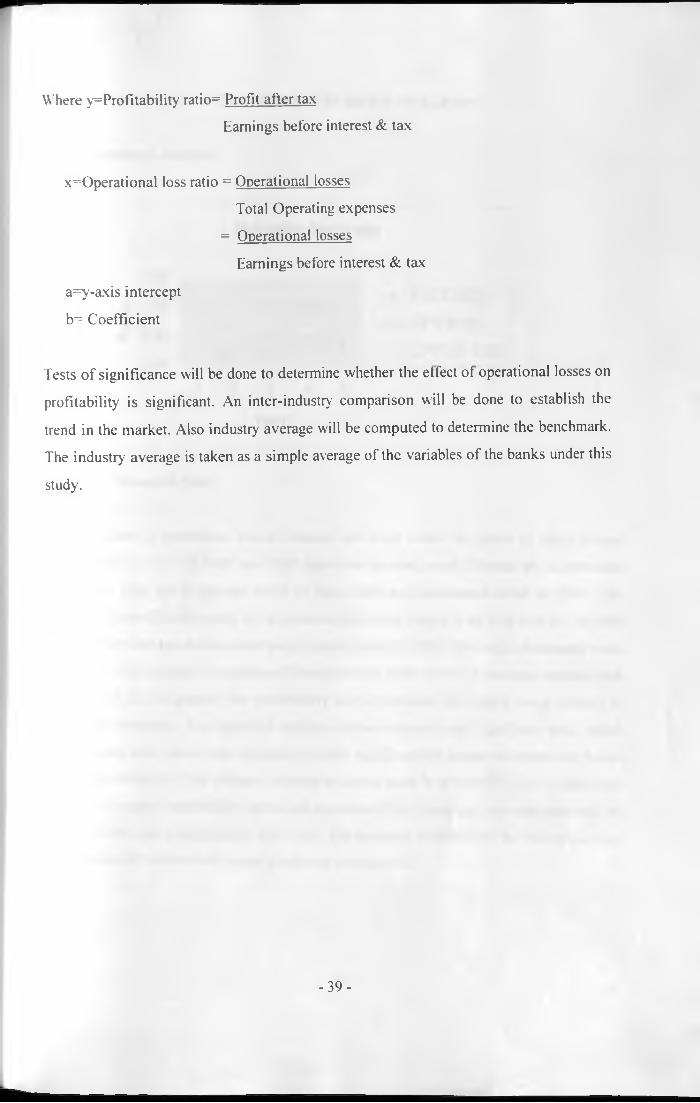
Where y=Profitability ratio= Profit after tax
Earnings before interest & tax
x=Operational loss ratio = Operational losses
Total Operating expenses
= Operational losses
Earnings before interest & tax
a=y-axis intercept
b= Coefficient
Tests o f significance will be done to determine whether the effect of operational losses on
profitability is significant. An inter-industry comparison will be done to establish the
trend in the market. Also industry average will be computed to determine the benchmark.
The industry average is taken as a simple average of the variables of the banks under this
study.
- 39 -

CHAPTER FOUR: DATA ANALYSIS
4.1.1 Industry Analysis
The industry’s operational losses earnings risk level under the period o f study ranged
from 0.79 to 1.31. In 2001 and 2002 there was upward trend followed by a downward
trend in year 2003, upward trend in year 2004 and downward trend in 2005. The
industry's profitability level in the period of this study ranged from 0.20 to 0.52. In 2001
and 2002 there was a downward trend, upward trend in 2003,2004 and a downward trend
in 2005. The industry’s operational losses level to total operating expenses ranged from
0.56 to 0.60. In general the profitability and operational loss ratios were moving in
opposite direction. The statistical analysis shows r-squares and significant tests, which
are greater than zero a clear indication of how significant the impact of operational losses
is on profitability. The industry average equation used is Y=a+b*X. The variables are
period of study, profitability ratios and operational loss ratios i.e. a=y-axis intercept, b=
Coefficient and x=operational loss ratio. The industry Y=0.661-0.275x shows that any
change in (x) variable will cause a negative change in Y.
- 4 0 -

4.1.2 African Banking Corporation
ABC
(0£
Year
+-PAT/EBU(I) ■*—OP/EBIT(l)
OP/T OP EX(I) -x— PAT/EBIT(b)
OP/EBIT(b) -•—OP/TOP EX(b)
Source: Research Data
The bank’s operational losses earnings risk level under the period of study ranged from
1.07 to 1.58 whereas the industry average ranged from 0.79 to 1.31. This shows that the
bank's operational losses level was high compared to industry average. In 2001,2002 and
2003 there is upward trend followed by a downward trend in years 2004 and 2005. The
bank’s profitability level in the same period ranged from 0.12 to 0.40 whereas the
industry average ranged from 0.20 to 0.52. In 2001, 2002 and 2003 there is upward trend
followed by a downward trend in years 2004 and 2005. The bank’s operational losses
level to total operating expenses ranged from 0.43 to 0.60 whereas the industry level
ranged from 0.56 to 0.60. In terms o f operating expenses the bank was doing well but for
other areas under study it was doing below average. The statistical analysis shows r-
squares and significant tests, which are greater than zero a clear indication of how
significant the impact of operational losses is on profitability. The overall industry shows
the same results of significance as the individual banks. The study shows a bank equation
of Y=-0.092+0.279x
-41 -

4.1.3 Bank of Baroda
Bank of Baroda
-♦— PAT/EBIT(I)
*-O P /E B IT (l)
OP/T OP EX(I)
*-PA T/EB IT(b)
— OP/EBIT(b)
OP/T OP EX(b)
Source: Research Data
The bank’s operational losses earnings risk level under the period of study ranged from
1.07 to 1.58 whereas the industry average ranged from 0.58 to 1.38. This shows that the
bank’s operational losses level was lower in years 2002, 2003, 2004 and 2005 but high in
2001 compared to industry average. The bank’s profitability level in the same period
ranged from 0.13 to 0.47 whereas the industry average ranged from 0.20 to 0.52. In 2001
and 2002 shows a steady trend, 2003 and 2004 upward trend followed by a downward
trend in year 2005. The bank's operational losses level to total operating expenses ranged
from 0.31 to 0.44 whereas the industry level ranged from 0.56 to 0.60. In terms of
operating expenses the bank was doing well but for other areas under study it was doing
below average. The statistical analysis shows r-squares and significant tests, which are
greater than zero a clear indication o f how significant the impact o f operational losses is
on profitability. The overall industry shows the same results o f significance as the
individual banks. The study shows a bank equation of Y=-0.548-0.314x.
-42-
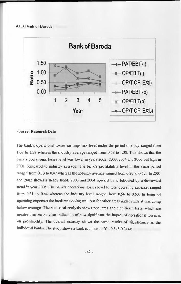
4.1.3 Bank of Baroda
Bank of Baroda
*-P A T/E B IT(l)
*-O P /E B IT (l)
OP/TOP EX(I)
— PAT/EBIT(b)
OP/EBIT(b)
^ -O P /T O P EX(b)
Source: Research Data
The bank's operational losses earnings risk level under the period of study ranged from
1.07 to 1.58 whereas the industry average ranged from 0.58 to 1.38. This shows that the
bank’s operational losses level was lower in years 2002, 2003, 2004 and 2005 but high in
2001 compared to industry average. The bank’s profitability level in the same period
ranged from 0.13 to 0.47 whereas the industry average ranged from 0.20 to 0.52. In 2001
and 2002 shows a steady trend, 2003 and 2004 upward trend followed by a downward
trend in year 2005. The bank’s operational losses level to total operating expenses ranged
from 0.31 to 0.44 whereas the industry level ranged from 0.56 to 0.60. In terms of
operating expenses the bank was doing well but for other areas under study it was doing
below average. The statistical analysis shows r-squares and significant tests, which are
greater than zero a clear indication o f how significant the impact o f operational losses is
on profitability. The overall industry shows the same results of significance as the
individual banks. The study shows a bank equation of Y=-0.548-0.314x.
Year
-42-
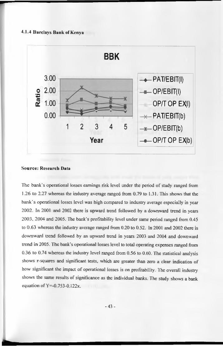
4.1.4 Barclays Bank of Kenya
BBK
♦-PA T/EB IT (I)
* -O P /E B IT (l)
OP/T OP EX(I)
*-P A T /E B IT (b )
^— OP/EBIT(b)
4 - OP/T OP EX(b)
Source: Research Data
The bank’s operational losses earnings risk level under the period o f study ranged from
1.26 to 2.27 whereas the industry average ranged from 0.79 to 1.31. This shows that the
bank 's operational losses level was high compared to industry average especially in year
2002. In 2001 and 2002 there is upward trend followed by a downward trend in years
2003, 2004 and 2005. The bank’s profitability level under same period ranged from 0.45
to 0.63 whereas the industry average ranged from 0.20 to 0.52. In 2001 and 2002 there is
downward trend followed by an upward trend in years 2003 and 2004 and downward
trend in 2005. The bank’s operational losses level to total operating expenses ranged from
0.36 to 0.74 whereas the industry level ranged from 0.56 to 0.60. The statistical analysis
shows r-squares and significant tests, which are greater than zero a clear indication of
how significant the impact o f operational losses is on profitability. The overall industry
shows the same results of significance as the individual banks. The study shows a bank
equation of Y=-0.753-0.122x.
-43-
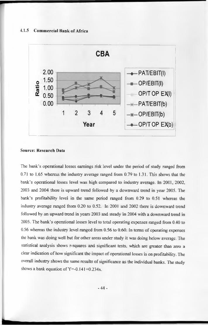
4.1.5 Commercial Bank of Africa
CBA
♦— PAT/EBIT(I)* —OP/EBIT(l)
OP/T OP EX(I) * —PAT/EBIT(b) * —OP/EBIT(b) ♦—OP/TOP EX(b)
Source: Research Data
The bank’s operational losses earnings risk level under the period of study ranged from
0.71 to 1.65 whereas the industry average ranged from 0.79 to 1.31. This shows that the
bank’s operational losses level was high compared to industry average. In 2001, 2002,
2003 and 2004 there is upward trend followed by a downward trend in year 2005. The
bank’s profitability level in the same period ranged from 0.29 to 0.51 whereas the
industry average ranged from 0.20 to 0.52. In 2001 and 2002 there is downward trend
followed by an upward trend in years 2003 and steady in 2004 with a downward trend in
2005. The bank’s operational losses level to total operating expenses ranged from 0.40 to
0.56 whereas the industry level ranged from 0.56 to 0.60. In terms of operating expenses
the bank was doing well but for other areas under study it was doing below average. The
statistical analysis shows r-squares and significant tests, which are greater than zero a
clear indication o f how significant the impact o f operational losses is on profitability. The
overall industry shows the same results of significance as the individual banks. The study
shows a bank equation of Y=-0.141 +0.234x.
- 4 4 -
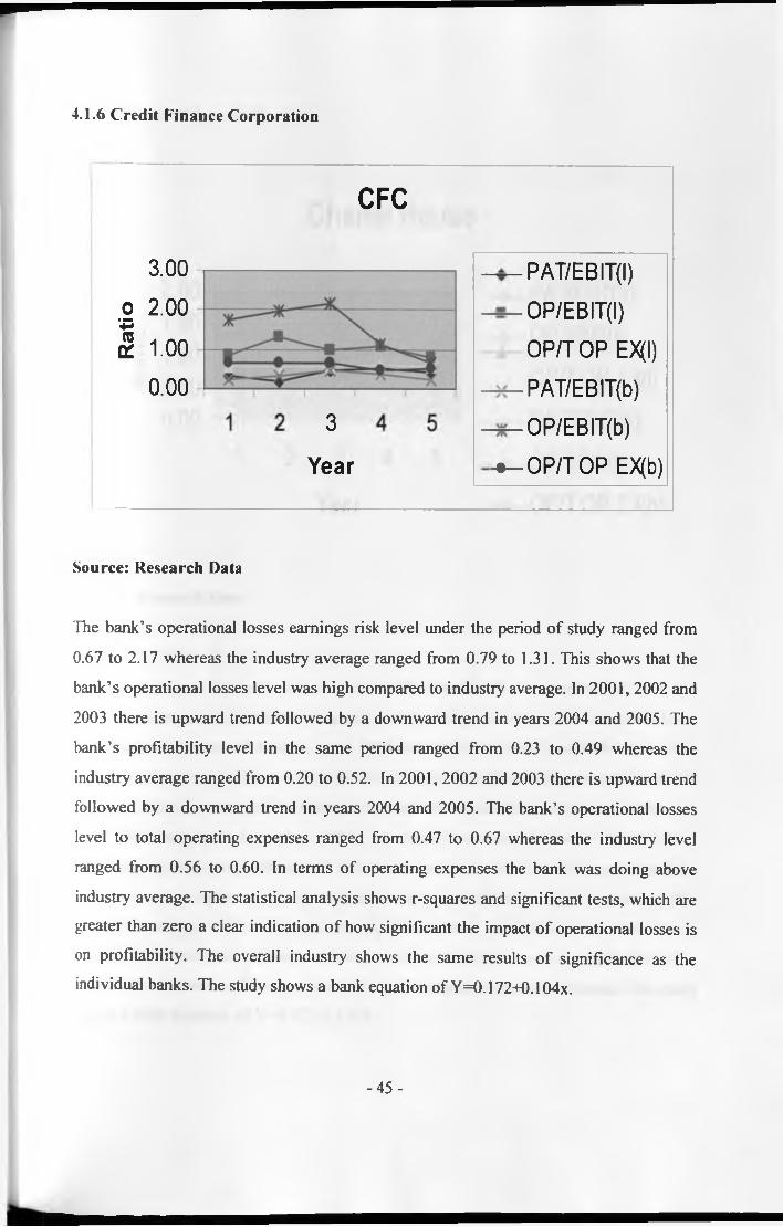
4.1.6 Credit Finance Corporation
CFC
3.000 2.00
■ mm
1 1.00 0.00
3
Year
PA77EBIT(I) 0P/EBIT(l) OP/T OP EX[I)
PAT/EBIT(b)— OP/EBIT(b)
-•— OP/TO P EX(b)
Source: Research Data
The bank’s operational losses earnings risk level under the period of study ranged from
0.67 to 2.17 whereas the industry average ranged from 0.79 to 1.31. This shows that the
bank’s operational losses level was high compared to industry average. In 2001,2002 and
2003 there is upward trend followed by a downward trend in years 2004 and 2005. The
bank’s profitability level in the same period ranged from 0.23 to 0.49 whereas the
industry average ranged from 0.20 to 0.52. In 2001, 2002 and 2003 there is upward trend
followed by a downward trend in years 2004 and 2005. The bank’s operational losses
level to total operating expenses ranged from 0.47 to 0.67 whereas the industry level
ranged from 0.56 to 0.60. In terms of operating expenses the bank was doing above
industry average. The statistical analysis shows r-squares and significant tests, which are
greater than zero a clear indication o f how significant the impact o f operational losses is
on profitability. The overall industry shows the same results o f significance as the
individual banks. The study shows a bank equation of Y=0.172+0.104x.
-45-

4.1.7 Charter House Bank
Charter House
(0O'
2.001.501.000.500.00
Year
PAT/EBIT(I)
OP/EBIT(l)
OP/TOP EX(I)
-x— PAT/EBIT(b)
— OP/EBIT(b)
-^ -O P /T O P EX(b)
Source: Research Data
The bank’s operational losses earnings risk level under the period of study ranged from
0.43 to 1.58 whereas the industry average ranged from 0.79 to 1.31. This shows that the
bank’s operational losses level in years 2001, 2002 and 2003 were low and in 2004 and
2005 high compared to industry average. In 2001, 2002 and 2003 there is upward trend
followed by a downward trend in years 2004 and 2005. The bank’s profitability level in
the same period ranged from 0.19 to 0.38 whereas the industry average ranged from 0.20
to 0.52. In 2001, 2002 and 2003 there is upward trend followed by a downward trend in
year 2004 and upward trend in 2005. The bank's operational losses level to total
operating expenses ranged from 0.53 to 0.77 whereas the industry level ranged from 0.56
to 0.60. In terms of operating expenses the bank was doing above industry average. The
statistical analysis shows r-squares and significant tests, which are greater than zero a
clear indication o f how significant the impact of operational losses is on profitability. The
overall industry shows the same results of significance as the individual banks. The study
shows a bank equation of Y=0.427-0.146x.
- 4 6 -

4.1.8 Chase Bank
C hase B ank
Y e a r
- P A T /E B IT (I)
m - O P /E B IT (l)
O P /T O PEX(I)
P A T /E B IT (b )
- O P /E B IT (b )
—• —- O P /T O PSource: Research Data
The bank’s operational losses earnings risk level under the period o f study ranged from
-5.28 to 2.28 whereas the industry average ranged from 0.79 to 1.31. The study shows
that the bank’s operational losses level was high in 2001, low in 2002, high in 2003, low
in 2004 and high in 2005 compared to industry average. The trend kept interchanging a
sign o f high-risk exposure. The bank trend in 2001 and 2002 showed a downward trend
followed by an upward trend in year 2003, an extreme downward trend in 2004 followed
by an upward trend in 2005. The bank’s profitability level in the same period ranged from
0.30 to 0.44 whereas the industry average ranged from 0.20 to 0.52. In 2001, 2002 and
2003 the bank was doing above average a good sign but in years 2004 and 2005 below
average. The bank’s operational losses level to total operating expenses ranged from 0.50
to 0.75 whereas the industry level ranged from 0.56 to 0.60. In terms of operating
expenses the bank was doing well except in year 2004. The statistical analysis shows r-
squares and significant tests, which are greater than zero a clear indication of how
significant the impact of operational losses is on profitability. The overall industry shows
the same results o f significance as the individual banks. The study shows a bank equation
of Y=0.579-0.137x.
- 4 7 -
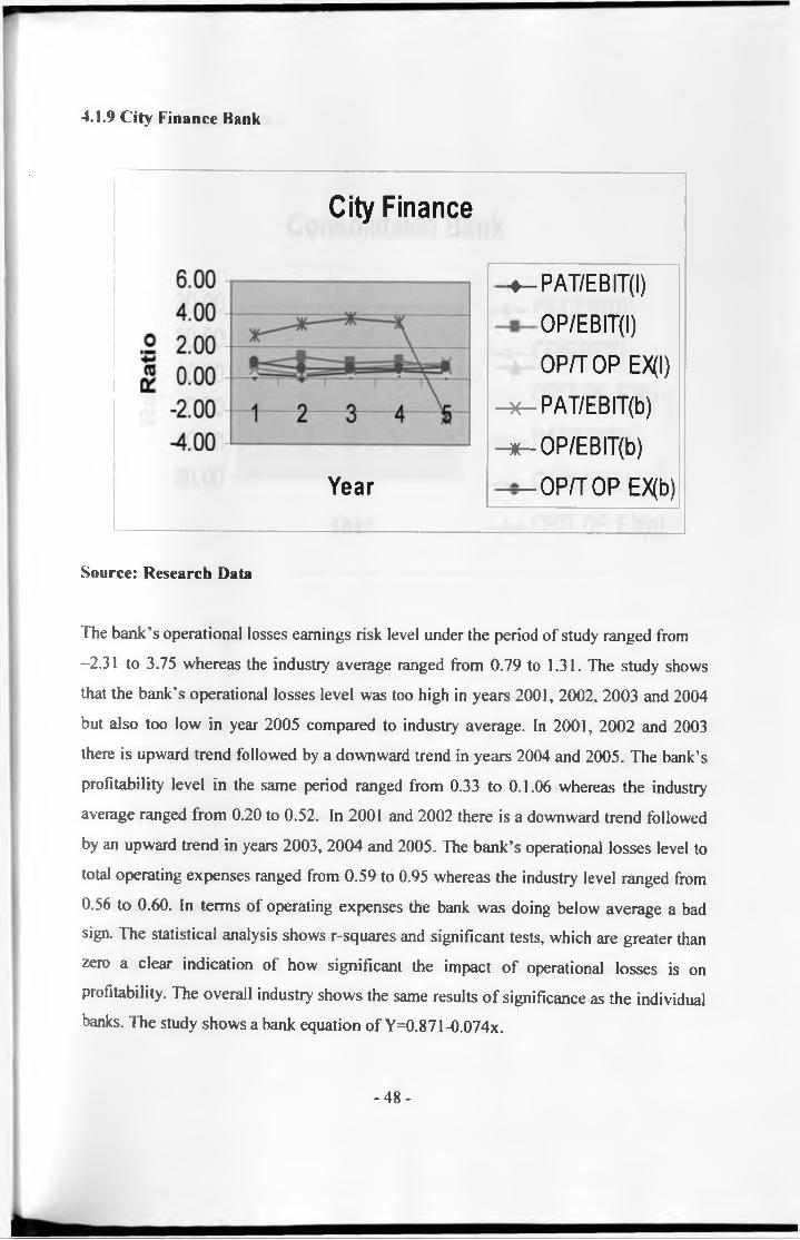
4.1.9 City Finance Bank
City Finance
Year
+-PAT/EBIT(I)
OP/EBIT(l)
OP/TOP EX(I)
*-PA T/EB IT(b)
*-O P /E B iT (b )
OP/TOP EX(b)
Source: Research Data
The bank’s operational losses earnings risk level under the period of study ranged from
-2.31 to 3.75 whereas the industry average ranged from 0.79 to 1.31. The study shows
that the bank's operational losses level was too high in years 2001, 2002, 2003 and 2004
but also too low in year 2005 compared to industry average. In 2001, 2002 and 2003
there is upward trend followed by a downward trend in years 2004 and 2005. The bank’s
profitability level in the same period ranged from 0.33 to 0.1.06 whereas the industry
average ranged from 0.20 to 0.52. In 2001 and 2002 there is a downward trend followed
by an upward trend in years 2003, 2004 and 2005. The bank’s operational losses level to
total operating expenses ranged from 0.59 to 0.95 whereas the industry level ranged from
0.56 to 0.60. In terms of operating expenses the bank was doing below average a bad
sign. The statistical analysis shows r-squares and significant tests, which are greater than
zero a clear indication of how significant the impact o f operational losses is on
profitability. The overall industry shows the same results of significance as the individual
banks. The study shows a bank equation of Y=0.871-0.074x.
- 4 8 -

4.1.10 Consolidated Bank
Consolidated Bank
30.0020.00
.2 10.000.00
- 10.00 - 20.00
<0k
1- 2 “ 3
Year
-*— PAT/EBIT(l)
OP/EBIT(l)
OP/TOP EX(I)
-*-PAT/EBIT(b)
-#-OP/EBIT(b)
-♦ -O P /TO P EX(b)
Source: Research Data
The bank’s operational losses earnings risk level under the period of study ranged from
-8.48 to 22.99 whereas the industry average ranged from 0.79 to 1.31. This shows that
the bank’s operational losses level was high compared to industry average. In 2002
downward trend followed by upward trend in years 2003, 2004 and 2005. The bank’s
profitability level in the same period ranged from -0.67 to 1.43 whereas the industry
average ranged from 0.20 to 0.52. In 2001, 2002, 2003 and 2004 there is upward trend
followed by a downward trend in year 2005. The bank’s operational losses level to total
operating expenses ranged from 0.54 to 0.76 whereas the industry level ranged from 0.56
to 0.60. The statistical analysis shows r-squares and significant tests, which are greater
than zero a clear indication of how significant the impact of operational losses is on
profitability. The overall industry shows the same results o f significance as the individual
banks. The study shows a bank equation o f Y=0.683-0.065x.
- 4 9 -

4.1.11 Co-operative Bank
Co-op Bank
-♦— PAT/EBIT(I)* —OP/EBIT(l)
OP/TOP EX(I) * —PAT/EBIT(b) * —OP/EBIT(b)♦ - OP/TOP EX(b)
Source: Research Data
The bank’s operational losses earnings risk level under the period o f study ranged from
2.07 to 5.60 whereas the industry average ranged from 0.79 to 1.31. This shows that the
bank’s operational losses level was too high compared to industry average. In 2002shows
an upward trend followed by a downward trend in years 2003 and 2004 with a downward
trend in 2005. The bank’s profitability level in the same period ranged from -1.27 to 0.22
whereas the industry average ranged from 0.20 to 0.52. In 2001, 2002, 2003 and 2004
there is upward trend followed by a downward trend in year 2005. The bank’s operational
losses level to total operating expenses ranged from 0.43 to 0.60 whereas the industry
level ranged from 0.56 to 0.60. In terms of operating expenses the bank was doing well
but for other areas under study it was doing below average. The statistical analysis shows
r-squares and significant tests, which are greater than zero a clear indication of how
significant the impact of operational losses is on profitability. The overall industry shows
the same results o f significance as the individual banks. The study shows a bank equation
of Y=l.l 15-0.353x.
- 5 0 -

4.1.12 Credit Bank
& 0.50 0.00
Credit Bank
3
Year
—♦ --P A T /E B IT (I)
-O P /E B IT (l)
O P /T O P EX(I)
—X - PAT/EBIT(b)
—X --O P /E B IT (b )
—• - -O P /T O P EX(b)
Source: Research Data
The bank’s operational losses earnings risk level under the period o f study ranged from
0.41 to 1.07 whereas the industry average ranged from 0.79 to 1.31. This shows that the
bank's operational losses level was high in 2003 but lower in years 2001, 2002, 2004 and
2005 compared to industry average. In 2001, 2002 and 2003 there is upward trend
followed by a downward trend in year 2004 with upward trend 2005. The bank's
profitability level in the same period ranged from 0.19 to 0.31 whereas the industry
average ranged from 0.20 to 0.52. In 2002 there is downward trend followed by an
upward trend in year 2003, downward trend in 2004 and upward trend 2005. The bank’s
operational losses level to total operating expenses ranged from 0.36 to 1.17 whereas the
industry level ranged from 0.56 to 0.60. In terms of operating expenses the bank was
doing well except in years 2004 and 2005. The statistical analysis shows r-squares and
significant tests, which are greater than zero a clear indication of how significant the
impact of operational losses is on profitability. The overall industry shows the same
results o f significance as the individual banks. The study shows a bank equation of
Y=0.320-0.063x.
-51 -

4.1.13 Development Bank
Development Bank
*-PAT/EBIT(l) a—0P/EBIT(l)
OP/TOP EX(I) *-PAT/EBIT(b) *-0P/EBIT(b)♦ -OP/TOP EX(b)
Source: Research Data
The bank's operational losses earnings risk level under the period o f study ranged from
0.71 to 2.01 whereas the industry average ranged from 0.79 to 1.31. This shows that the
bank's operational losses level was high in years 2001, 2002 and 2003 but low in 2004
and 2005 compared to industry average. In 2001 and 2002 there is upward trend followed
by a downward trend in years 2003, 2004 and 2005. The bank’s profitability level in the
same period ranged from 0.16 to 0.52 whereas the industry average ranged from 0.20 to
0.52. The study shows an upward trend in all the years a good sign o f improvement. The
bank’s operational losses level to total operating expenses ranged from -0.16 to 0.73
whereas the industry level ranged from 0.56 to 0.60. In terms of operating expenses the
bank was doing well. The statistical analysis shows r-squares and significant tests, which
are greater than zero a clear indication of how significant the impact o f operational losses
is on profitability. The overall industry shows the same results of significance as the
individual banks. The study shows a bank equation of Y=0.666-0.257x.
- 52 -

4.1.14 Diamond Trust
The bank’s operational losses earnings risk level under the period o f study ranged from
0.08 to 1.48 whereas the industry average ranged from 0.79 to 1.31. This shows that the
bank’s operational losses level was high compared to industry average. In 2001, 2002,
2003 and 2004 there is upward trend followed by a downward trend in year 2005. The
bank's profitability level in the same period ranged from 0.13 to 0.41 whereas the
industry average ranged from 0.20 to 0.52. In 2001,2002 and 2003 there is upward trend
followed by a downward trend in years 2004 and 2005. The bank’s operational losses
level to total operating expenses ranged from 0.34 to 0.49 whereas the industry level
ranged from 0.56 to 0.60. In terms o f operating expenses the bank was doing well above
average. The statistical analysis shows r-squares and significant tests, which are greater
than zero a clear indication o f how significant the impact of operational losses is on
profitability. The overall industry shows the same results o f significance as the individual
banks. The study shows a bank equation o f Y=-0.052+0.295x.
-53-
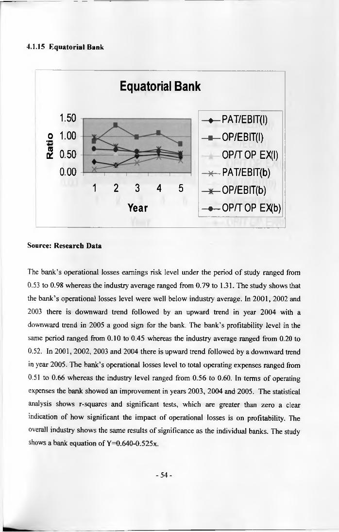
4.1.15 Equatorial Bank
Equatorial Bank
1.50
o 1.00a m
S 0.50
0.001 2 3 4 5
Year
4— PAT/EBIT(I)
* — 0P/EBIT(l)
OP/T OP EX(I)
^— PAT/EBIT(b)
* — 0P/EBIT(b)
^ OP/T OP EX(b)
Source: Research Data
The bank’s operational losses earnings risk level under the period o f study ranged from
0.53 to 0.98 whereas the industry average ranged from 0.79 to 1.31. The study shows that
the bank’s operational losses level were well below industry average. In 2001, 2002 and
2003 there is downward trend followed by an upward trend in year 2004 with a
downward trend in 2005 a good sign for the bank. The bank’s profitability level in the
same period ranged from 0.10 to 0.45 whereas the industry average ranged from 0.20 to
0.52. In 2001, 2002, 2003 and 2004 there is upward trend followed by a downward trend
in year 2005. The bank’s operational losses level to total operating expenses ranged from
0.51 to 0.66 whereas the industry level ranged from 0.56 to 0.60. In terms o f operating
expenses the bank showed an improvement in years 2003, 2004 and 2005. The statistical
analysis shows r-squares and significant tests, which are greater than zero a clear
indication of how significant the impact of operational losses is on profitability. The
overall industry shows the same results of significance as the individual banks. The study
shows a bank equation of Y=0.640-0.525x.
- 54 -

4.1.16 Equity Bank
Source: Research Data
The bank’s operational losses earnings risk level under the period o f study ranged from
1.33 to 2.90 whereas the industry average ranged from 0.79 to 1.31. The study shows that
the bank’s operational losses level were above the industry average. In 2002, 2003 and
2004 there was an upward trend followed by a downward trend in year 2005. The bank’s
profitability level in the same period ranged from 0.36 to 0.59 whereas the industry
average ranged from 0.20 to 0.52. The study shows an improvement in terms of
profitability above industry average. The bank’s operational losses level to total operating
expenses ranged from 0.45 to 0.60 whereas the industry level ranged from 0.56 to 0.60.
The statistical analysis shows r-squares and significant tests, which are greater than zero a
clear indication of how significant the impact of operational losses is on profitability. The
overall industry shows the same results o f significance as the individual banks. The study
shows a bank equation of Y=0.265+0.093x.
- 55 -

4.1.17 Fina Bank
The bank’s operational losses earnings risk level under the period of study ranged from
0.61 to 4.24 whereas the industry average ranged from 0.79 to 1.31. This shows that the
bank’s operational losses level was low in years 2001, 2002 and 2003 but high in 2004
and 2005 compared to industry average. In 2001, 2002, 2003 and 2004 there was upward
trend followed by a downward trend in year 2005. The bank’s profitability level in the
same period ranged from -0.35 to 0.21 whereas the industry average ranged from 0.20 to
0.52. The study shows a poor performance of the bank compared to industry average. The
bank's operational losses level to total operating expenses ranged from 0.16 to 0.71
whereas the industry level ranged from 0.56 to 0.60. The statistical analysis shows r-
squares and significant tests, which are greater than zero a clear indication of how
significant the impact of operational losses is on profitability. The overall industry shows
the same results o f significance as the individual banks. The study shows a bank equation
of Y=0.231-0.133x.
-56-

4.1.18 First American Bank
First American Bank
O'
2.001.50
1.000.50
0.003
Year
-PAT/EBIT(I)- m - -0P/EBIT(l)
OP/T OP EX(I)
—x - PAT/EBIT(b)
—X --0P/EBIT(b)
-O P/TO P EX(b)
Source: Research Data
The bank’s operational losses earnings risk level under the period of study ranged from
0.67 to 1.68 whereas the industry average ranged from 0.79 to 1.31. This shows that the
bank's operational losses level was low in year 2001 and 2002, high in 2003, 2004 and
2005 compared to industry average. In 2001, 2002 and 2003 there is upward trend
followed by a downward trend in years 2004 and 2005. The bank’s profitability level in
the same period ranged from 0.29 to 0.44 whereas the industry average ranged from 0.20
to 0.52. In 2002, 2003 and 2004 there is upward trend followed by a downward trend in
year 2005. The bank's operational losses level to total operating expenses ranged from
0.43 to 0.57 whereas the industry level ranged from 0.56 to 0.60. In terms o f operating
expenses the bank was doing well but for other areas under study it was doing below
average. The statistical analysis shows r-squares and significant tests, which are greater
than zero a clear indication o f how significant the impact of operational losses is on
profitability. The overall industry shows the same results o f significance as the individual
banks. The study shows a bank equation o f Y=0.228+0.097x.
- 57 -
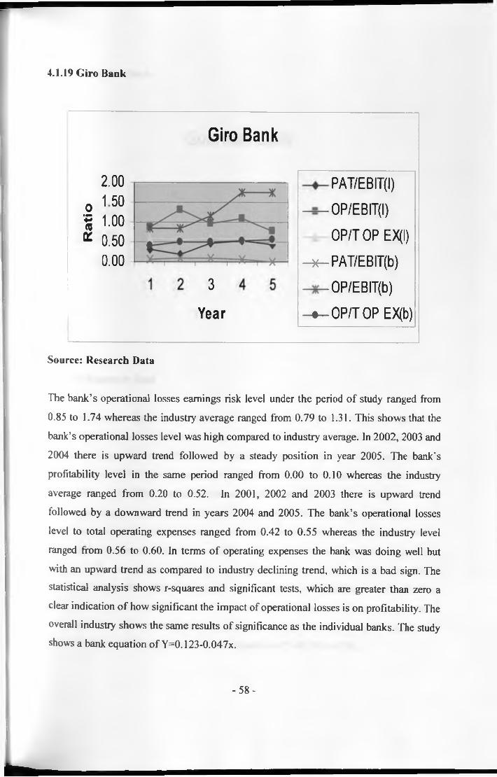
4.1.19 Giro Bank
Giro Bank
2.00 o 1 50S tooK 0.50 ,
0.003
Year
PAT/EBIT(I)
OP/EBIT(l)
OP/T OP EX(I)
-x— PAT/EBIT(b)
OP/EBIT(b)
-•— OP/TOP EX(b)
Source: Research Data
The bank’s operational losses eamings risk level under the period o f study ranged from
0.85 to 1.74 whereas the industry average ranged from 0.79 to 1.31. This shows that the
bank’s operational losses level was high compared to industry average. In 2002,2003 and
2004 there is upward trend followed by a steady position in year 2005. The bank's
profitability level in the same period ranged from 0.00 to 0.10 whereas the industry
average ranged from 0.20 to 0.52. In 2001, 2002 and 2003 there is upward trend
followed by a downward trend in years 2004 and 2005. The bank’s operational losses
level to total operating expenses ranged from 0.42 to 0.55 whereas the industry level
ranged from 0.56 to 0.60. In terms o f operating expenses the bank was doing well but
with an upward trend as compared to industry declining trend, which is a bad sign. The
statistical analysis shows r-squares and significant tests, which are greater than zero a
clear indication o f how significant the impact of operational losses is on profitability. The
overall industry shows the same results of significance as the individual banks. The study
shows a bank equation o f Y=0.123-0.047x.
- 58 -
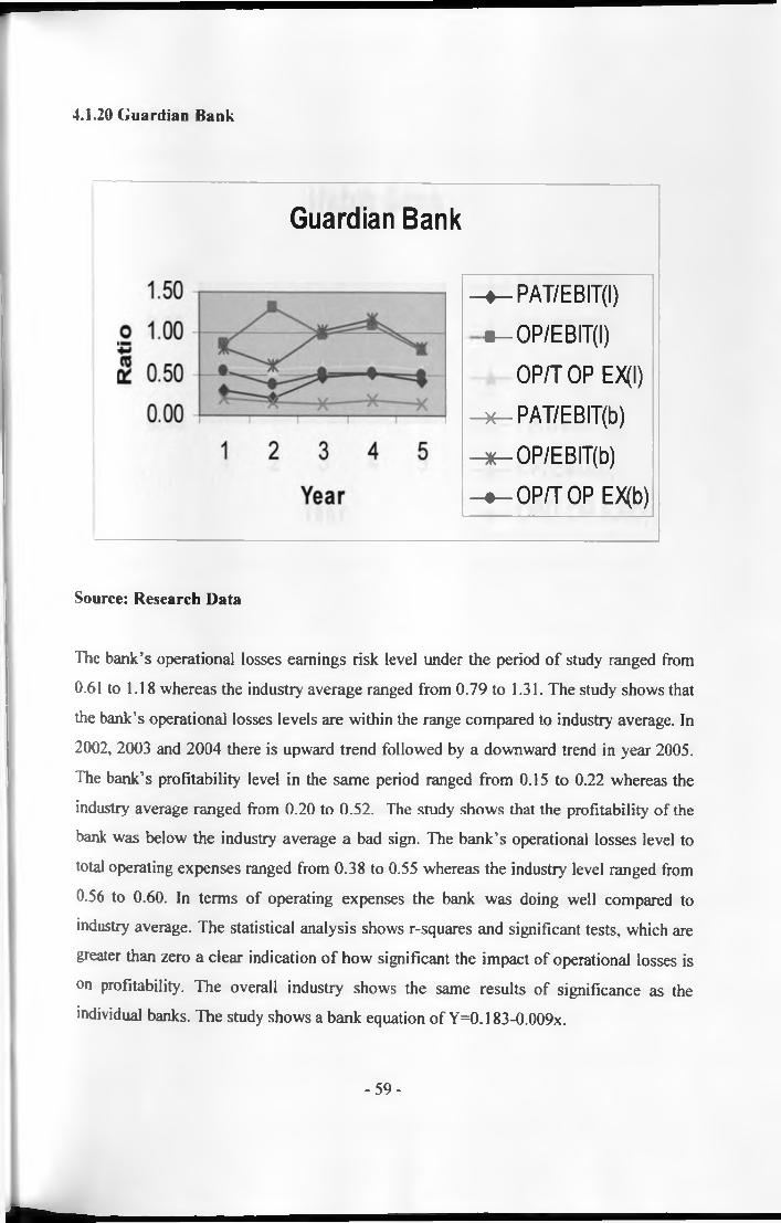
4.1.20 Guardian Bank
Guardian Bank
♦ —PAT/EBIT(I)
* — OP/EBIT(l)
OP/T OP EX(I)
* — PAT/EBIT(b)
* — 0P/EBIT(b)
♦ - OP/T OP EX(b)
Source: Research Data
The bank’s operational losses earnings risk level under the period o f study ranged from
0.61 to 1.18 whereas the industry average ranged from 0.79 to 1.31. The study shows that
the bank’s operational losses levels are within the range compared to industry average. In
2002, 2003 and 2004 there is upward trend followed by a downward trend in year 2005.
The bank’s profitability level in the same period ranged from 0.15 to 0.22 whereas the
industry average ranged from 0.20 to 0.52. The study shows that the profitability of the
bank was below the industry average a bad sign. The bank’s operational losses level to
total operating expenses ranged from 0.38 to 0.55 whereas the industry level ranged from
0.56 to 0.60. In terms of operating expenses the bank was doing well compared to
industry average. The statistical analysis shows r-squares and significant tests, which are
greater than zero a clear indication of how significant the impact of operational losses is
on profitability. The overall industry shows the same results of significance as the
individual banks. The study shows a bank equation of Y=0.183-0.009x.
-59-

4.1.21 Habib Bank
The bank’s operational losses earnings risk level under the period o f study ranged from
0.56 to 2.19 whereas the industry average ranged from 0.79 to 1.31. This shows that the
bank’s operational losses level was high compared to industry average. The study shows
an upward trend for all the years under study. The bank’s profitability level in the same
period ranged from 0.19 to 0.52 whereas the industry average ranged from 0.20 to 0.52.
In 2001, 2002, 2003 and 2004 there is upward trend followed by a downward trend in
year 2005. The bank’s operational losses level to total operating expenses ranged from
0.26 to 0.41 whereas the industry level ranged from 0.56 to 0.60. In terms of operating
expenses the bank was doing well as compared to industry average. The statistical
analysis shows r-squares and significant tests, which are greater than zero a clear
indication of how significant the impact o f operational losses is on profitability. The
overall industry shows the same results o f significance as the individual banks. The study
shows a bank equation of Y=0.437-0.086x.
- 60 -

4.1.22 Habib A. G Zurich
Habib A. G Zurich
♦~PAT/EBIT(I)
* — OP/EBIT(l)
OP/T OP EX(I)
^— PAT/EBIT(b)
*-O P /E B IT (b )
OP/T OP EX(b)
Source: Research Data
The bank’s operational losses earnings risk level under the period o f study ranged from
0.81 to 2.16 whereas the industry average ranged from 0.79 to 1.31. The study shows that
the bank’s operational losses level was high except year 2002 compared to industry
average. In 2002, 2003 and 2004 there is upward trend followed by a downward trend in
year 2005. The bank's profitability level in the same period ranged from 0.26 to 0.47
whereas the industry average ranged from 0.20 to 0.52. The bank’s profitability level
was below industry average a bad sign for the bank. The bank’s operational losses level
to total operating expenses ranged from 0.39 to 0.51 whereas the industry level ranged
from 0.56 to 0.60. In terms o f operating expenses the bank was doing well as compared
to industry average. The statistical analysis shows r-squares and significant tests, which
are greater than zero a clear indication o f how significant the impact o f operational losses
is on profitability. The overall industry shows the same results of significance as the
individual banks. The study shows a bank equation of Y=0.228+0.108x.
-61 -

4.1.23 I & M
The banks operational losses earnings risk level under the period o f study ranged from
0.54 to 1.03 whereas the industry average ranged from 0.79 to 1.31. This shows that the
bank’s operational losses level was lower compared to industry average. In 2001, 2002,
2003 and 2004 there is upward trend followed by a downward trend in year 2005. The
bank’s profitability level in the same period ranged from 0.13 to 0.40 whereas the
industry average ranged from 0.20 to 0.52. The bank's profitability level was below
industry average a bad sign for the bank. In 2001, 2002, 2003 and 2004 there is upward
trend followed by a downward trend in year 2005. The bank's operational losses level to
total operating expenses ranged from 0.56 to 0.68 whereas the industry level ranged from
0.56 to 0.60. In terms of operating expenses the bank was doing well compared to
industry average. The statistical analysis shows r-squares and significant tests, which are
greater than zero a clear indication o f how significant the impact of operational losses is
on profitability. The overall industry shows the same results of significance as the
individual banks. The study shows a bank equation of Y=-0.117+0.493x.
- 62 -
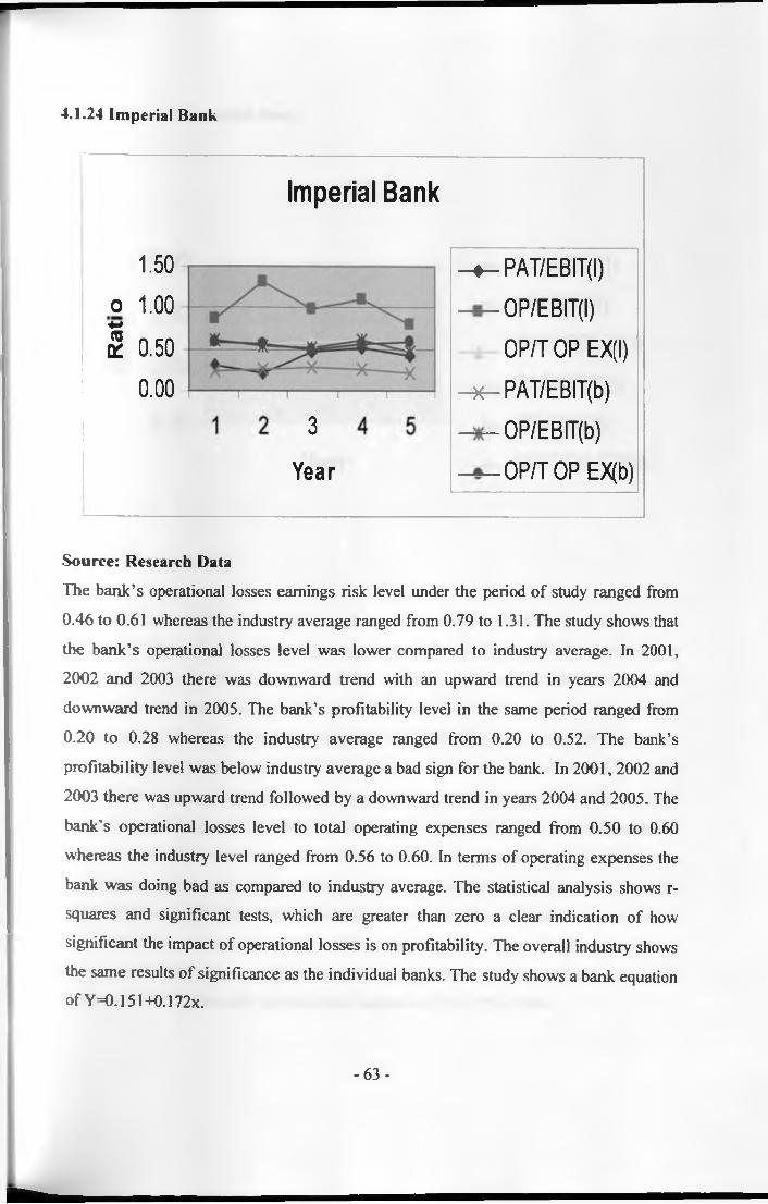
4.1.24 Imperial Bank
Imperial Bank
1.50
0 1.001 0.50
0.003
Year
-♦— PAT/EBIT(I)
OP/EBIT(l)
OPIT OP EX(I)
-x-PAT/EBIT(b)
OP/EBIT(b)
OP/T OP EX(b)
Source: Research Data
The bank’s operational losses earnings risk level under the period o f study ranged from
0.46 to 0.61 whereas the industry average ranged from 0.79 to 1.31. The study shows that
the bank’s operational losses level was lower compared to industry average. In 2001,
2002 and 2003 there was downward trend with an upward trend in years 2004 and
downward trend in 2005. The bank’s profitability level in the same period ranged from
0.20 to 0.28 whereas the industry average ranged from 0.20 to 0.52. The bank’s
profitability level was below industry average a bad sign for the bank. In 2001, 2002 and
2003 there was upward trend followed by a downward trend in years 2004 and 2005. The
bank's operational losses level to total operating expenses ranged from 0.50 to 0.60
whereas the industry level ranged from 0.56 to 0.60. In terms of operating expenses the
bank was doing bad as compared to industry average. The statistical analysis shows r-
squares and significant tests, which are greater than zero a clear indication of how
significant the impact of operational losses is on profitability. The overall industry shows
the same results of significance as the individual banks. The study shows a bank equation
of Y=0.151+0.172x.
- 63 -

4.1.25 Kenya Commercial Bank
KCB
-PAT/EBIT(I)
-0P/EBIT(l)
OP 11 OP EX(I)
PAT/EBIT(b)
-0P/EBIT(b)
-0 P /T 0 P EX[b)
Source: Research Data
The bank’s operational losses earnings risk level under the period of study ranged from
-4.35 to 4.77 whereas the industry average ranged from 0.79 to 1.31. The study shows
that the bank’s operational losses level was too high compared to industry average but
with slight improvement in year 2005. In 2001,2002 and 2004 there was an upward trend
followed by a downward trend in years 2003 and 2005. The bank’s profitability level in
the same period ranged from 0.13 to 0.56 whereas the industry average ranged from 0.20
to 0.52. The bank’s profitability level was above industry average except 2001 and 2003
a good sign for the bank. The bank’s operational losses level to total operating expenses
ranged from 0.44 to 0.68 whereas the industry level ranged from 0.44 to 0.68. There was
an improvement in terms of operating expenses compared to industry average in years
2003, 2004 and 2005. The statistical analysis shows r-squares and significant tests, which
are greater than zero a clear indication o f how significant the impact o f operational losses
is on profitability. The overall industry shows the same results of significance as the
individual banks. The study shows a bank equation of Y=0.755-0.099x.
- 64 -

4.1.26 Middle East Bank
Middle East Bank
2.00 —♦— PAT/EBIT(I)1.00
0 -m - 0P/EBIT(l)i 0 . 0 0 A---' ' \ X ~— —r~ —r~---- V ---- 1------- OP/T OP EX(I)“ -1.00
\COCNI PAT/EBIT(b)-2.00 - — 0P/EBIT(b)
Year - • — OP/TOP EX(b)
Source: Research Data
The bank’s operational losses earnings risk level under the period of study ranged from
-0.78 to 1.76 whereas the industry average ranged from 0.79 to 1.31. The study shows
that the bank's operational losses level was high in years 2003 and 2004 but low in 2001,
2002 and 2005 compared to industry average. In 2001, 2002,2003 and 2004 there is
upward trend followed by a downward trend in year 2005. The bank’s profitability level
in the same period ranged from 0.20 to 0.33 whereas the industry average ranged from
0.20 to 0.52. The bank’s profitability level was below industry average a bad sign for the
bank. The bank’s operational losses level to total operating expenses ranged from 0.40 to
0.64 whereas the industry level ranged from 0.56 to 0.60. The trend was not bad when
compared to industry average. The statistical analysis shows r-squares and significant
tests, which are greater than zero a clear indication of how significant the impact of
operational losses is on profitability. The overall industry shows the same results of
significance as the individual banks. The study shows a bank equation o f Y=0.259-
0.007x.
- 65 -
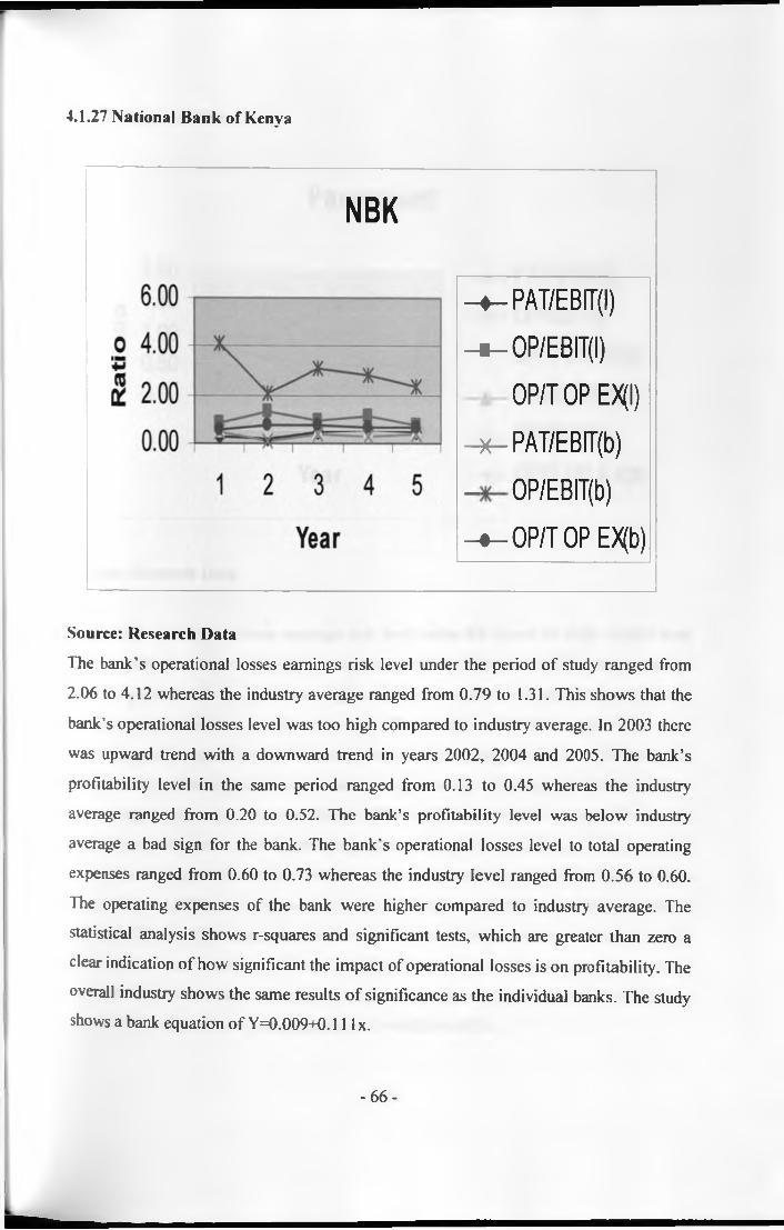
4.1.27 National Bank of Kenya
NBK
—«— PAT/EBIT(I)—■— 0P/EBIT(l)
OP/TOP EX(I)
—x— PAT/EBIT(b)— 0P/EBIT(b) - 4- OP/TOP EX(b)
Source: Research Data
The bank’s operational losses earnings risk level under the period of study ranged from
2.06 to 4.12 whereas the industry average ranged from 0.79 to 1.31. This shows that the
bank’s operational losses level was too high compared to industry average. In 2003 there
was upward trend with a downward trend in years 2002, 2004 and 2005. The bank’s
profitability level in the same period ranged from 0.13 to 0.45 whereas the industry
average ranged from 0.20 to 0.52. The bank’s profitability level was below industry
average a bad sign for the bank. The bank's operational losses level to total operating
expenses ranged from 0.60 to 0.73 whereas the industry level ranged from 0.56 to 0.60.
The operating expenses of the bank were higher compared to industry average. The
statistical analysis shows r-squares and significant tests, which are greater than zero a
clear indication o f how significant the impact of operational losses is on profitability. The
overall industry shows the same results o f significance as the individual banks. The study
shows a bank equation o f Y=0.009+0.111 x.
- 66 -

4.1.28 Paramount Bank
Paramount
TOCC.
2.001.50
1.000.50
0.003
Year
-PAT/EBIT(I)
-0P/EBIT(l)
OP/TOP EX(I)
—X - PAT/EBIT(b)
—x --0P/EBIT(b)
-OP/TO P EX(b)
Source: Research Data
The bank’s operational losses earnings risk level under the period of study ranged from
0.94 to 1.65 whereas the industry average ranged from 0.79 to 1.31. This shows that the
bank’s operational losses level was high compared to industry average. The study shows
an upward trend for the years under study. The bank’s profitability level in the same
period ranged from 0.07 to 0.15 whereas the industry average ranged from 0.20 to 0.52.
The bank’s profitability level was below industry average a bad sign for the bank. There
was a slight improvement in years 2002, 2003 and 2004 but below average. The bank’s
operational losses level to total operating expenses ranged from 0.49 to 0.75 whereas the
industry level ranged from 0.56 to 0.60. In terms of operating expenses the bank badly in
year 2001 and 2002 but improved in years 2003, 2004 and 2005 compared to industry
average. The statistical analysis shows r-squares and significant tests, which are greater
than zero a clear indication o f how significant the impact o f operational losses is on
profitability. The overall industry shows the same results o f significance as the individual
banks. The study shows a bank equation o f Y=0.023+0.075x.
- 6 7 -

w
4.1.29 Standard Charted Bank
Source: Research Data
The bank’s operational losses earnings risk level under the period of study ranged from
0.71 to 1.22 whereas the industry average ranged from 0.79 to 1.31. The study shows that
the bank’s operational losses level was low compared to industry average. In 2001 and
2002 there was upward trend followed by a downward trend in years 2003 with upward
trend in 2004 followed by a downward movement in 2005. The bank’s profitability level
in the same period ranged from 0.49 to 0.61 whereas the industry average ranged from
0.20 to 0.52. The profitability was good compared to industry. The bank’s operational
losses level to total operating expenses ranged from 0.47 to 0.54 whereas the industry
level ranged from 0.56 to 0.60. In terms o f operating expenses the bank was doing well
above industry average. The statistical analysis shows r-squares and significant tests,
which are greater than zero a clear indication of how significant the impact of operational
losses is on profitability. The overall industry shows the same results o f significance as
the individual banks. The study shows a bank equation of Y=0.427+0.141x.
- 6 8 -

4.130 Stanbic Bank
Source: Research Data
The bank's operational losses earnings risk level under the period of study ranged from
0.79 to 9.03 whereas the industry average ranged from 0.79 to 1.31. The study shows that
the bank's operational losses level were high compared to industry average. There is no
clear trend. The bank’s profitability level in the same period ranged from -2.47 to 0.53
whereas the industry average ranged from 0.20 to 0.52. The bank's operational losses
level to total operating expenses ranged from 0.44 to 0.66 whereas the industry level
ranged from 0.56 to 0.60. In terms o f operating expenses the bank was doing well
compared to industry average. The statistical analysis shows r-squares and significant
tests, which are greater than zero a clear indication of how significant the impact of
operational losses is on profitability. The overall industry shows the same results of
significance as the individual banks. The study shows a bank equation of Y=0.860- 0.304x.
- 69 -

4.131 Transnational Bank
The bank's operational losses earnings risk level under the period of study ranged from
0.24 to 2.81 whereas the industry average ranged from 0.79 to 1.31. The study shows that
the bank’s operational losses level was high 2002, 2003 and 2005 but low in 2001 and
2004 compared to industry average. In 2001, 2002 and 2003 there is upward trend
followed by a downward trend in year 2004 with upward movement in 2005. The bank's
profitability level in the same period ranged from 0.46 to 0.98 whereas the industry
average ranged from 0.20 to 0.52. The profitability level was stable except in 2005,
which is a bad sign for the bank. The bank’s operational losses level to total operating
expenses ranged from 0.42 to 0.55 whereas the industry level ranged from 0.56 to 0.60.
In terms o f operating expenses the bank was doing well compared to industry average.
The statistical analysis shows r-squares and significant tests, which are greater than zero a
clear indication of how significant the impact of operational losses is on profitability. The
statistical analysis shows r-squares and significant tests, which are greater than zero a
clear indication of how significant the impact of operational losses is on profitability. The
overall industry shows the same results o f significance as the individual banks. The study
shows a bank equation of Y=1.096-0.201 x.
- 70 -
CHAPTER FIVE: SUMMARY OF FINDINGS, CONCLUSIONS,
RECOMMENDATIONS, LIMITATIONS OF STUDY AND
SUGGESTIONS FOR FURTHER STUDY
5.1 Summary Findings, and Conclusions
5.1.1 Summary Findings
This study was conducted w ith the aim of achieving the objectives of analyzing the level
and trend o f operational losses of commercial banks in Kenya and determining whether
there is a significant impact of operational losses on profitability' of commercial banks in
Kenya.
To achieve the above objectives, profitability and operational losses ratio w'ere computed.
Industry average was computed by taking the simple average o f variables under research
for 30 commercial banks. The trend was then compared with the change in the industry
average, the operational and profitability ratios over the period 2001 to 2005.
The study results reveal that the profitability of commercial banks is affected by
operational losses and there exists an inverse relationship between profitability and
operational losses of commercial banks o f Kenya. The above findings can be explained
by looking at the big banks and mostly government owned and foreign owned banks.
Where lower operational losses ratio were noticed there was increased profitability.
The relationship between profitability and level of operational losses was found to be
direct and positive for most commercial banks whereas some had negative relationship.
The relationship was found to be significant. The category most affected is the big banks
mostly government owned commercial banks. The large foreign owned banks indicated
lower significance levels as compared to large locally owned commercial banks. The
foreign owned small commercial banks indicated a lower significance level as compared
to small locally owned commercial banks.
-71 -

The statistical analysis and significance tests show a value greator than zero, which is a
good sign that the operational losses have a direct relationship with the level of
profitability. This study shows r-square of 0.195. t-test of 2.010 and significance level of
0.729. The overall industry shows the same results of significance as the individual
banks. The equation used is Y=a+b*X. The variables are period of study, profitability
ratios and operational loss ratios.
a=y-axis intercept
b= Coefficient
This study’s statistical analysis shows an industry equation o f Y=0.661-0.275x. This
study shows that any change in (x) variable will cause a negative change in (Y). The
constant variable 0.661 is the profitability ratio representing the profit that is not affected
by change in operational loss ratio whereas the variable -0.275 represents coefficient
factor. The industry equation gives a clear indication of the effect of operational losses on
profitability in the banking industry.
5.1.2 Conclusions
The result o f this study is consistent with findings of other researchers about the effect of
operational losses on profitability. This study shows that the impact of operational losses
on profitability of commercial banks is significant as opposed to general believe that the
impact o f operational losses on profitability of commercial banks is not significant.
5.2 Limitations of the Study
Granted that the data used in this study was obtained from published financial statements,
one must be cautious o f the limitations associated with such data. This data may, to some
degree be manipulated by the management o f a firm to present a “ rosy" view of the firms
position. This kind of manipulation is known as “window dressing". The possibility of
window dressing has been controlled to some extent by use o f many commercial banks.
-72-

There was a limitation due to lack o f data for some commercial banks reducing the banks
under study to 30 instead of 44.
The figures o f operational losses may include non-operational losses for the same
commercial banks, as there is no clear demarcation between operational losses and
operating expenses used directly in generation of revenue. This study was undertaken
within a fixed duration and the researcher did not have adequate time to explore aspects
like dynamic ratios, w hich reflect day-to-day operations of the commercial banks.
5.3 Recommendations
Commercial banks should put more emphasis on operational losses management as it
affects their profitability. For Central Bank, being the regulator should put strong
mechanisms to monitor commercial banks operational risk exposure and if need be
require them to submit operational risk exposure quarterly returns. There is need to
include detailed operational loss variables in the financial statements to facilitate accurate
judgment when assessing the profitability o f commercial by its stakeholders.
5.4 Suggestions For Further Study
A study based on dynamic operational losses and profitability ratio analysis is hereby
recommended. This study will establish the day-to-day impact of operational losses on
profitability o f commercial banks. A study on other industries on same variables could be
undertaken. Another study can be done on each of the variables separately over a longer
period o f time with more than two ratios. A further study can be done to test how' the
efficiency levels affect profitability of commercial banks.
- 73 -

REFERENCES
British Bankers' Association. (1999). Operational Risk, the Next Frontier.
Davies. P., (2000), Fraud Watch. KPMB. 2nd Edition London
Basel Committee, (1998), "Framework for the Internal Controls Systems in Banking
Organizations". September BIS BASEL
Rose P. S.(1997), “Money and Capital Markets. Financial Institutions and Instruments in
a Global Marketplace" Sixth edition Irw in.
Credit Suisse Group (2003) "Operational Risks in Financial Services" April Report
Payle D (1997) "Bank Risk Management -Working paper No. 272", University of
California
Basel Committee, Risk Management Group (2000), "Other Risks (OR) Discussion
Paper" April BIS, BASEL.
Doering FLU (2003), "Operational Risk in Financial Services” Report, April FSA
(2000).
FSA 2000. Consultation Paper 46"Money Laundering: the FSA’s New Role", London.
April report.
Basel Committee, (1996). Payment and Settlement Systems, "Settlement Risk in Foreign
Exchange Transactions" BIS BASEL March.
Dickinson. G. (2000), "Insurance Finds a Blend of Innovation and Tradition" Financial
Times, June.
- 74 -
Kimball. R. (2000). “Failures in Risk Management" New England Economic Review.
January/ February.
Kimber. M. (2000), "Finding Value in a Collection of Losses" Operational Risk Manager
June.
Philippe Jorion, (1997) "Value at Risk" Second Edition McGraw-Hill.
Jameson, R (1998), “Operational Risk and Financial Institutions” Arthur Andersen. UK.
Meridien Research Inc. (2000), "Time for a New Look at Operational Risk" New York.
Morris, S. (2000), "Operational Risk Control, What FSA Expects... and You Must Do"
London.
Samad-Khan et al (1998), "Measuring Operational Risk" Global Trading, Quarter 4.
Jameson, R. (1998), "On the Quantification of Operational Risk” Operational Risk and
Financial Institutions. Risk Books. London A Short Polemic in.
The Daily Nation (June. 2005) "Banks Fail Test on Risk Control".
The Daily Nation (February to April 2002. 2003. 2004 and 2005) “Financial Statement
Publications”
Rachlin. C. (1998), "Operational Risk in Retail Banking" in Jameson. R. Operational
Risk and Financial Institutions, Risk Books. London.
Senior, A. (1999), "A Modem Approach to Operational Risk" Risk Professional. Issue
1/3 May.
- 75 -

p
Thiessen. K. (2000), "Don't Gamble with Goodwill" the Conference Board o f Canada.
Report.
Young. B. (2000), "Quantification of Operational Risk" Center for Operational Risk
Research & Education.
Yussuf A. Idarus (2005), “Survey of Operational Risks Management Practices by
Commercial Banks in Kenya” U.O.N Unpublished MBA Project.
Wachira W. (1999), “ An Analysis of the Relationship Between Liquidity and
Macroeconomic Indicators: An Inter Industry Comparison' U.O.N Unpublished MBA
Project.
Hennie V. G. and Bratanovic. B. (1999), “ Analyzing Banking Risk" World Bank
Publication on.
-76-

VV
APPEDICES
A l.l List of Commercial Banks
4
5
6
7
8
9
10
11
12
13
14
15
16
17
18
19
20
21
22
23
24
25
26
27
African Banking Corporation
Akiba Bank Ltd
Bank o f Baroda
Bank o f India
Barclays Bank of Kenya Ltd
CFC Bank Limited
Charterhouse Bank Limited
Chase Bank Limited
Citibank. N.A.
City Finance Bank
Commercial Bank of Africa
Consolidated Bank of Kenya
Co-operative Bank of Kenya
Credit Bank Limited
Development Bank of Kenya
Diamond Trust Bank Kenya
Dubai Bank Limited
Equatorial Commercial Bank
Equity Bank Limited
Fidelity Commercial Bank
Fina Bank Limited
First American Bank Limited
Giro Commercial Bank
Guardian Bank
Habib AG Zurich
Habib Bank Limited
Imperial Bank Limited
- 77 -

28
29
30
31
32
33
34
35
36
37
38
39
40
41
42
43
44
Industrial Development Bank
Investment & Mortgages Bank
Kenya Commercial Bank Ltd
K-Rep Bank
Middle East Bank of Kenya
National Bank of Kenya Ltd
National Industrial Credit Bank
Paramount-Universal Bank
Prime Bank Limited
Southern Credit Banking Corp.
Stanbic Bank Kenya Limited
Standard Chartered Bank Ltd
Transnational Bank Limited
Victoria Commercial Bank Ltd
Daima Bank Limited
Oriental comm bank
Bank of Africa
- 78 -

TABLE OF RESEARCH DATATotal
Operational operating Earnings Beforey r Losses expenses Interest & Tax Earnings After tax PAT/EBIT OP/EBIT OPfT OP EX
c 2001 144.89 2 4 2 2 4 227.44 27.57 0 12 1 07 0 6 0
c 2002 95 86 202 19 184.63 30.10 0 16 1 10 0 47
c 2003 138.83 255 88 162.17 44.70 0 28 1 58 0 54
c 2004 110.09 253 86 194.18 78.12 0 4 0 1 31 0 43
c 2005 145.69 305 64 263.20 81.72 0,31 1 16 0 48
'k of B a r o d a 2001 86.53 277 34 201.34 25.63 0 13 1 38 031
r* o f B a r o d a 2002 99.97 306 28 246.68 32.01 0 13 1 24 0 33
m of B a r o d a 2003 104.56 2 7 9 5 3 383.63 97.62 0.25 0 7 3 0 37
n t of B a r o d a 200 4 134.47 307 14 431.69 201.76 0 4 7 0.71 0.44
nk o f B a r o d a 2005 131.76 311 09 540.55 165.65 0 31 0 58 0 42
X 2001 4 ,330 .00 7,027.00 5,593.00 2,955.00 0 53 1 26 0 62
X 2002 3 ,198 51 8,944 00 3,934.00 1,783.00 0 45 2.27 0.36
X 2003 5,745.00 9,152.00 5,653.00 3,367.00 0 60 1 62 0 6 3
K 2004 6,140.00 8.316.00 5,857.00 3,715.00 0 6 3 1.42 07 4
K 2005 6.082.00 8,824.00 6,361.00 3,721.00 0 58 1.39 0 6 9
3A 2001 317.01 787 48 1,112.72 353.74 0.32 0.71 04 0
M 2002 409.81 880.93 853.57 250.21 0 2 9 1.03 0 47
3A 2003 549.26 9 8 3 9 4 780.53 396.72 0 51 1 26 0 56
3A 2004 483.40 920 56 556.57 282.20 0.51 1.65 0 5 3
BA 2005 620.37 1,294 04 1,241.20 511.41 041 1 04 0 4 8
PC 2001 870.47 1,322 85 771.80 191.82 0 2 5 1.71 0 6 6
PC 2002 881.26 1.337.53 681.98 224.73 0.33 1 96 0 6 6
FC 2003 1,130.30 1,696 01 781.90 382.05 0 49 2 17 0 6 7
FC 2004 355.87 760 15 687.39 242.44 0 35 1 11 0 4 7
FC 2005 453.75 853 01 1,271.29 295.71 0.23 0 6 7 0 5 3
' i t e r t t o u s e 2001 63.61 84 53 194.95 64.04 0 33 0 43 0 7 5
:‘ a r !e it io iis e 2002 81.94 112 48 204.99 72.68 0 35 0 55 0 73
.ta rte rh o u s e 2003 103.09 14869 197.45 74.60 0 38 0 75 0 6 9
lu r te rt io u s e 2004 182.59 237 78 150.63 28.04 0 19 1 58 0 77
P o r te rh o u s e 2005 112.24 211 47 265.97 77.13 0 2 9 0 80 C 53
P a s e 2001 117.31 213.62 93.80 38.75 0.41 2 28 C 55
:hase 2002 39.10 78.10 80.01 32.16 0.40 0 98 0 50
Ihase 2003 47.52 9 2 7 8 91.28 40.27 0 4 4 1 02 0 51
> a s e 2004 200.86 26661 (50.50) (67.12) 1 33 (5 2 8 ) 0 7 5
> -a se 2005 77.85 156 06 142.51 42.79 0 30 1.10 0 50
City F in a n c e 2001 61.38 64 94 24.08 14.90 0 6 2 2.70 0 95
City F in a n c e 2002 40.38 57 94 17.08 5.66 0 33 3 39 0 70
City F in a n c e 2003 35.65 54 54 14.55 9.47 0.65 3.75 0 65
City F in a n c e 2004 26.69 45 06 12.89 11.40 0 88 3 50 0 59
City F in a n c e 2005 83.19 102 64 (44.48) (47.00) 1 06 (2.31) 0 81
C o n s o lid a te d 2001 184.93 317 19 58.54 (13.14) (0.22) 5 4 2 0 5 8
C o n s o lid a te d 2002 428.23 561 94 144.87 77.20 0 53 3.88 0 76
C o n s o lid a te d 2003 251.47 444 82 51.74 12.17 0 2 4 8 60 0 5 7
C o n s o lid a te d 2004 228.47 420 88 (49.65) (71.02) 1 43 (8 48) 0.54
C o n s o lid a te d 2005 232.41 4 3 2 8 7 18.83 (12.66) (067) 22 99 0 54
C o-op B a n k 2001 1,802.79 2,858 22 510.78 (651.01) (127 ) 5 60 0 63
C o-op B a n k 2002 1,702.33 2.819 98 1,280.30 164.78 0 13 2 20 0 6 0
C o -o p B a n k 2003 1,725.72 2.963 53 883.39 154.99 0 18 3 35 0 58
C o-op B a n k 2004 2,468.24 3.821 70 922.06 206.61 0.22 4 14 0 65
C o-op B a n k 2005 2,945.35 4 ,55323 2,204.47 439.96 0 2 0 2 07 0 65
Credit 2001 50.26 97 25 129.62 37.62 0 29 0.75 0 52
Credit 2002 38.40 10531 115.20 21.95 0 19 0 91 0 36
Credit 2003 52.61 123 60 115.10 34.23 0 30 1.07 0 4 3
Credit 2004 54.87 47 08 114.84 32.68 0 28 0 41 1.17
C’B dit 2005 62.58 8 9 8 6 199.54 62.28 0.31 0 4 5 0 70
79

0 510 730 430 66
(0 16)0 340 390 470 490540660 630 570 590 510 600450 520 570 490 530660630 710 160 430 570 520 450 570 420 510 500 530 550 550 380 520510480 410 370 410260380.510 440 450 390 400 630 680 630 620560 600 570 500 56
2001 145.01 28262 178.00 28.79 0 16 1 592002 280 28 381 62 189.63 41.57 022 2012003 78.93 182 70 186.60 69.91 0 37 0 982004 63.92 93 55 131.89 65.40 0 50 0 712005 ( 26 .35) 166 00 220.81 115.62 0 52 0 752001 106.93 312 38 307.89 40.93 0 13 1 012002 133.05 338 01 309.21 75.53 0 24 1 092003 211.77 447 11 342.03 139.24 041 1.312004 280.29 577.58 389.71 147.34 0 38 1 482005 418.41 77049 965.51 248.88 0.26 0 802001 106.28 162 20 166.25 17.40 0 10 0 982002 95.45 152 54 208.65 43.92 0.21 0 732003 76.45 133.12 239.05 65.14 027 0 562004 61.30 103.32 155.25 69.91 045 0 672005 55.98 109 04 205.23 71.02 0.35 0 532001 196.69 326.32 184.54 65.75 0 36 1 772002 116.55 256 75 192.58 74.24 0 39 1 332003 217.72 420.35 210.51 97.31 046 2 002004 465.62 817.51 281.75 136.14 0 48 2 902005 642.52 1.302.21 582.86 344.60 0 59 2 232001 131.33 245 60 403.70 7.01 002 0 612002 196.83 296 66 413.15 45.90 0.11 0 722003 198.55 314 62 356.30 74.75 021 0 882004 364.41 514 31 121.34 (42.22) (0 .35) 4 242005 54.70 344 80 347.55 61.03 0 18 0 992001 151.69 350 34 520.57 154.66 0 30 0 672002 231.28 408 63 409.04 118.76 0 29 1 002003 215.67 417 46 248.36 85.33 034 1 682004 231.20 510.10 340.70 150.23 044 1 502005 235.28 412.63 413 04 138 74 0 34 1 002001 97.78 235 46 275.04 16.68 006 0 862002 123.78 242 46 286.04 23.45 0 08 0 852003 122.04 244 15 213.00 21.50 0 10 1 152004 146.05 273 79 157.39 10.22 0 06 1 742005 180.98 328 00 188.22 0.88 0 00 1 742001 103.90 189 40 231.30 51.34 0 22 0 822002 57.82 154 12 252.71 43.26 0.17 0.612003 109.91 211.96 203.64 30.53 0.15 1 042004 111.41 219 74 186.13 33.95 0.18 1 182005 103.27 214 45 264.28 39.06 0.15 0 812001 56.32 136 28 245.00 78.08 0.32 0 562002 53.11 14324 232.28 76.85 0.33 0 622003 67.75 167 10 159.89 55.97 0.35 1.052004 35.07 136 58 121.19 63.54 0 52 1 132005 67.10 175.85 80.15 14.87 0 19 2 192001 99.57 195 07 210.40 61.70 0 29 0 932002 84.57 190 07 205.40 53.27 0 26 0 932003 82.07 181.68 140.99 52.45 037 1 292004 70.08 179 87 83.21 39.03 0 47 2.162005 74.99 189 48 233.08 95.06 041 0 812001 172.73 27470 507.54 68.16 0,13 0 542002 214.36 317 53 439.58 59.77 0 14 0.722003 332.54 523 95 580.67 195.08 0 34 0902004 400.85 651 05 634.82 254.65 0 40 1.032005 422.83 748 81 1,174.09 345.52 0 29 0 642001 156.04 261 22 435.24 101.64 0.23 0.602002 159.60 27946 512.28 127.38 0 25 0 552003 155.25 31276 616.44 175.02 0.28 0.512004 244.32 434 77 708.42 184.37 0.26 061
80

0 590 610680 490 480 440 400 530640540 560 600 700 730 700 670 750 630 530 490 540 470 500 540540 530 660 440 600 510 570 430 500 550 500 42
2005 281.29 473 84 1,030.56 205 54 020 0 462001 5 ,126.06 8,397 36 2,880 80 381.98 0 13 2912002 7 , 131.00 10.486 61 (2,411.10) (3 ,000.64) 1 24 (4 35)2003 3 ,235.85 6.602 41 1,694.19 485.52 0 29 3902004 3 ,259.32 6.76067 1,418.10 793.10 0 56 4 772005 3 ,053.64 6,93627 2,426.43 1.343.61 055 2862001 60.40 152 68 264.64 54.42 0 21 0 582002 83.69 158 71 202.35 40.04 0 20 0 782003 128.32 200 71 169.21 53.57 0 32 1 192004 (90.76) ( 167.12) 95.22 23.39 0.25 d 76)2005 (107.87) (186 21) 239.56 78.86 0 33 (0 78)2001 1 ,666.31 2.761 25 670.23 298.87 045 4.122002 2 ,150.42 3,058 10 1,485.51 198.76 0 13 2062003 2 ,492.86 3,434 72 1,127.23 403.90 036 3 052004 2 ,407.69 3.431 37 1,216.97 382.61 031 2822005 2 ,460.24 3,654 59 1,571.86 598.54 0 38 2 332001 58.51 78 26 82.92 9.56 0 12 0 942002 46.51 74 26 78.92 5.90 0 07 0942003 43.19 80 93 59.37 6.98 012 1 362004 41.73 8461 52.70 8.16 0 15 1.612005 59.15 108 97 65.85 9.28 0 14 1 652001 1,540.85 3.269 13 4 ,599.70 2,235.23 049 0712002 1,741.06 3,465 54 4,291.72 2,206.13 051 0812003 1,827.85 3 ,395.09 4 ,600.10 2,788.72 0.61 0 742004 1,999.17 3.689 17 3,033.40 1,832.18 0 60 1 222005 2 , 132.66 3.990 13 4,502.26 2 ,443.00 0 54 0 892001 433.12 652 86 85.38 (210.78) (247 ) 7652002 65.27 149 83 190.12 26.39 0 14 0 792003 437.64 730.53 80.88 ( 104.35) (1 29) 9 032004 365.98 720 43 212.07 109.98 0 52 3402005 563.93 982 42 555.62 291.95 0 53 1.772001 96.47 224 51 271.39 251.63 0 93 0 832002 113.48 226 30 156.56 134.18 0 86 1 452003 125.69 230.09 138.67 118.21 0 85 1 662004 124.87 248.15 1,052.27 1,035.98 098 0 242005 100.45 239 84 85.41 39.31 0 46 281
81

INKS TABLE OF RATIOSP A T/EB IT(I) O P /E B IT (l) O P /T OP E X (I) PAT/EBIT(b) O P /EB IT(b ) O P/T O P EX(b) b=y/x(i) b=y/x(b)
2001 0 3 2 0 8 6 0 .5 8 0 12 1 07 0 6 0 0 3 6 0 112 0 0 2 0 2 0 1.31 0 56 0 16 1 10 0 47 0 1 5 0 152 0 0 3 0 .46 0 9 8 0 .5 8 0 2 8 1 58 0 5 4 0 4 7 0 172 0 0 4 0 52 1 09 0 .6 0 0 4 0 1 31 0 4 3 0 4 7 0 312 0 0 5 0 4 3 0 7 9 0 .5 7 0.31 1.16 0 4 8 0 5 4 0 2 7
O ' B a ro d a PAT/EBITO ) O P /E B IT(t) O P /T OP E X (I) PAT/EBIT(b) O P /EB IT(b ) O P /T O P EX(b) b=y/x(i) b=y/x(b)2001 0 .32 0 8 6 0 .5 8 0.13 1 38 0.31 0 36 0 0 92 0 0 2 0 .20 1.31 0 .5 6 0 .13 1.24 0 3 3 0.15 0.102 0 0 3 0 .46 0 98 0 58 0 .25 0.73 0 37 0 4 7 0 3 52 0 0 4 0 .52 1 09 0 6 0 0 4 7 0 71 0 44 0 47 0 662 0 0 5 0 .43 0 7 9 0 .5 7 0.31 0.58 0 4 2 0 5 4 1 0 5 3
gK PAT/EBITO) O P /E B IT (l) O P /T OP E X (I) PAT/EBIT(b) O P /EB IT(b ) O P/T O P EX(b) b=y/x(i) b=y/x(b)2001 0 .32 0 8 6 0 58 0 .53 1 26 0 6 2 0 3 6 0.422 0 0 2 0 .20 1.31 0 .5 6 0 45 2 27 0 3 6 0 15 0 202 0 0 3 0 .4 6 0 9 8 0 .5 8 O 60 l 1.62 0.63 0 4 7 0 372 0 0 4 0 .52 1.09 0 .6 0 0 .63 1.42 0.74 0 4 7 0 4 52 0 0 5 0 .43 0.79 0 5 7 0.58 1.39 0.69 0 5 4 0 4 2
:a* PAT/EBITO) O P/EB ITfl) O P /T O P E X (I) PAT/EBIT(b) O P /EB IT(b ) OP/T O P EX(b) b=y/x(i) b=y/x(b)2001 0 .3 2 0.86 0 .5 8 0 32 0.71 0 4 0 0.36 0 4 52 0 0 2 0 .2 0 1.31 0 .5 6 0 2 9 1.03 0 4 7 0 1 5 0 282 0 0 3 0 .4 6 0.98 0 .5 8 0.51 1.26 0 5 6 0 4 7 0 4 02 0 0 4 0 52 1.09 0 .6 0 0.51 1.65 0.53 0 47 0 3 12 0 0 5 0 .4 3 0.79 0 .5 7 0.41 1.04 0.48 0 5 4 0 40
b e PA T/EB IT /I) O P/EB IT(l) O P /T O P E X (I) PAT/EBIT(b) O P /EB IT(b ) O P /T O P EX(b) b=y'*Q) b=y/x(b)2001 0 32 0.86 0 .5 8 0 .25 1.71 0 6 6 0.36 0.152 0 0 2 0 2 0 1.31 0 .5 6 0 .33 1.96 0.66 0.15 0.1720 03 0 4 6 0.98 0 .5 8 0.49 2.17 0 6 7 0.47 0 2 32 0 0 4 0 .5 2 1.09 0 .6 0 0.35 1.11 0 4 7 0.47 0.322 0 0 5 0 4 3 0.79 0 .57 0.23 0.67 0.53 0.54 0.35
o a r e r H ouse PAT/EBITO) O P /E B TO) O P /T O P E X (I) PAT/EBIT(b) O P /E B IT(b ) OP/T O P EX(b) b=y/x(i) b=y/x(b)2001 0 32 0 8 6 0 58 0 .33 0.43 0 7 5 0 3 6 0 762002 0 2 0 1.31 0 .56 0 .35 0 5 5 0 7 3 0.15 0 6 52003 0 4 6 0.98 0 .5 8 0 .38 0 7 5 0 6 9 0 4 7 0 502004 0 .5 2 1.09 0 .6 0 0 .19 1.58 0.77 0 4 7 0.122005 0 .4 3 0.79 0 .5 7 0 29 0 8 0 0.53 0 5 4 0 36
|> a s e Bank PAT/EBITO) OP/EBITO) O P /T O P E X (I) PAT/EBIT(b) O P /E B IT (b ) O P/T O P EX(b) b=y/x(.)____ b=y/x(b)2001 0 .3 2 0.86 0 .5 8 0.41 2 28 0 5 5 0 3 6 0 182002 0 .2 0 1.31 0 .5 6 0 4 0 0.98 0.50 0 1 5 0 4 12003 0 .4 6 0.98 0 .58 0 44 1 02 05 1 0 47 0 4 32004 0 .5 2 1.09 0 .6 0 1.33 -5.28 0.75 0 4 7 -0.252005 0 .4 3 0 .79 0 .57 0.30 1.10 0 5 0 0 54 0 2 7
p ty Finance PAT/EBITO) OP/EBITO) O P /T O P E X (I) PAT/EBIT(b) O P /E B IT (b ) O P/T O P EX(b) b=W*(i) b=y/x(b)2001 0 .3 2 0 86 0 .58 0.62 2 70 0 9 5 0 3 6 0.232002 0 .2 0 1.31 0 .5 6 0.33 3 3 9 0.70 0 15 0.102003 0 .4 6 0 9 8 0 .58 0 6 5 3.75 0.65 0.47 0.172004 0 .5 2 1.09 0 .60 0 8 8 3 50 0 59 0.47 0.252005 0 .4 3 0.79 0 .57 1.06 -2 3 1 0.81 0.54 -0.46
Jo-'sclidated PAT/EBITO) OP/EBITO) O P/T O P E X (I) PAT/EBIT(b) O P /E B IT (b ) O P/T O P EX(b) b=y/x(i) b=y/x(b)2001 0 .3 2 0 8 6 0 .58 -0.22 5 4 2 0.58 0.36 -0 042002 0 .2 0 1.31 0 .56 0 53 3 88 0.76 0.15 0.142003 0 .4 6 0 98 0 .58 0 2 4 8^60 0.57 0 4 7 0 0 32004 0 52 1.09 0.60 1.43 -8 .48 0.54 0.47 -0.172005 0 4 3 0 79 0 57 -0 6 7 22 .99 0.54 0.54 -0 03
82

■gank P A T /E B IT (I) O P /E B IT (l) O P /T O P EX(I) P A T/EB IT(b) O P /EB IT(b ) O P /T OP EX(b) b=y/x(i) b=y/x(b)2 0 0 1 0 .32 0 .86 0 5 8 -1.27 5 6 0 0 6 3 0 .36 -0 23
2 0 0 2 0 .20 1.31 0.56 0 13 2 2 0 0 6 0 0 15 0 06
" 2 0 0 3 0 4 6 0 .98 o"58l 0.18 3 35 0 58 0 47 0 05
2 0 0 4 0 .52 1.09 0.60 0 2 2 4 .1 4 0 6 5 0 4 7 0 05
2 0 0 5 0 4 3 0 .79 0.57 0 2 0 2 .0 7 0 .65 0 54 0 10
P A T /E B IT (I) O P /E B IT O ) O P /T O P EX(I) PA T/EB IT(b) O P /EB IT(b ) O P /T OP EX(b) b=y/x(i) b=y/x(b)
2 0 0 1 0 32 0 .86 0 58 0 29 0 .7 5 0 .52 0 36 0 39
2 0 0 2 0 .20 1.31 0.56 0.19 0.91 0 .36 0 15 0.21
2 0 0 3 0 .4 6 1 0 9 8 1 0 5 5 0.30 1.07 0 43 0 47 0 28
2 0 0 4 0 .52 1.09 0.60 0.28 0 41 1.17 0 47 0 69
2 0 0 5 0 .43 0 79 0.57 0 3 1 0 4 5 0 7 0 0 54 0 69
»c o ren t P A T /E B IT (I) O P /E B ITO ) O P /T O P EX(I) PA T/EB IT(b) O P /EB IT(b ) O P /T OP EX(b) b=y/x(i) b=y/x(b)_
2 0 0 1 0 .32 0.86 0.58 0.16 1 .59 0.51 0.36 0.10
2 0 0 2 0 20 1 31 0 56 0.22 2 01 0 .73 0.15 0.11
2 0 0 3 0.46 0.98 0.58 0.37 0 .9 8 0 4 3 0 47 0 38
2 0 0 4 0 52 1.09 0 6 0 0.50 0 7 1 0 68
2 0 0 5 0 .43 0.79 0 5 7 0.52 0 .7 5 -0 .16 0.54 0.70
P A T /F R lT (l) O P /E B IT (l) O P /T O P EX(I) PA T/EB IT(b) O P /E B IT(b ) O P /T OP EX(b) b=y/x(i) b=y/x(b)
20 01 0 32 0.86 0.58 0.13 1.01 0.34 0.36 0.13
2 0 0 2 0 20 1.31 0.56 0 2 4 1.09 0 39 0.15 0 . z z
2 0 0 3 0 46 0.98 0.58 04 1 1.31 0.47 0.47 0.31
2 0 0 4 0 52 1 09 0.60 0 38 1.48 0 49 0.47 0.2b
2 0 0 5 0 .43 0.79 0.57 0 26 0 80 0 54 0.54 0.32
j y i a l ____________ P A T /E B IT (I)0 32
O P /E B IT (l!0.86
O P /T OP EX< I!0 .58
PA T/EB IT(b)0.10
O P/EB IT(b)0 98
O P/T OP E X (b r 0 6 6
___0 36
b=y/x(b) 0 11
2 0 0 22 0 0 3
0 2 0 0 46
1.31 0 98
0 .560 .58
0.210.27
0 .7 30 .56
0.630.57
0.15 0 47 0.49
2 0 0 42 0 0 5
0 .520 4 3
1.090.79
0 .600.57
0.450.35
0 .670 .53
0.590.51
0.47 0 54
U.bo 0 65
83

3 T _ P A T /E B IT (I) O P /E B IT O ) OP/T O P EX(I) P A T /E B IT (b ) O P/EB IT(b) O P /T OP EX(b) b=y/x(i) b=y/x(b)_ 2 0 0 1 0 .32 0 8 6 0.58 0 2 2 0 .82 0 55 0 36 0 2 7_ 2 0 0 2 0 2 0 1.31 0.56 0.17 0 6 1 0 3 8 0.15 0.28_ 2 0 0 3 0 46 0 9 8 0 58 0.15 1 04 0 .52 0 47 0.14
2 0 0 4 0 5 2 1 09 0 6 0 0 18 1 18 0 51 0 47 0 152 0 0 5 0.43 0 .79 0.57 0.15 0 81 0 48 0.54 0 18
P A T /E B IT O ) O P /E B IT O ) O P/T O P EX(I) P A T /E B IT (b ) O P/EB IT(b) O P /T OP EX(b) b=y/x(i) b=y/x(b)2 0 0 1 0.32 0 8 6 0 5 8 0 3 2 0 56 0 4 1 0 36 0 572 0 0 2 0 2 0 1.31 0 56 0 3 3 0 62 0 37 0 .15 0 54
__________ 2 0 0 3 0 4 6 0.98 0.58 0.35 1.05 0 4 1 0 4 7 0 332 0 0 4 0 5 2 1.09 0.60 0 6 2 1 .13 0 .26 0 4 7 0 472 0 0 5 0 4 3 0 7 9 0.57 0 19 2 .1 9 0 38 0 5 4 0 08
t A G Z u r ic h P A T/E B ITO ) O P /E B IT (l) O P/T O P EX(I) P A T /E B IT(b ) O P/EB IT(b) O P /T OP EX(b) b=y/x(i) b=y/x(b)2 0 0 1 0.32 0.86 0.58 0 2 9 0 .9 3 0 51 0 3 6 0.32
___________ 2 0 0 2 0.20 1.31 0.56 0.26 0 .9 3 0 4 4 0.15 0.282 0 0 3 0.46 0.98 0 5 8 0.37 1.29 0 .45 0 .47 0.292 0 0 4 0 5 2 1.09 0 6 0 0 47 2 l 6 l 0 .39 0 4 7 0 222 0 0 5 0.43 0.79 0.57 0.41 0.81 0 .40 0 54 0.50
J P A T/EB ITO )
h-CD
yQ.O
O P /T O P EX(I) P A T/EB IT(b)
3(—CD
£o
O P /T OP EX(b) b=y/x(i) b=y/x(b)2 0 0 1 0.32 0 86 0 58 0.13 0 54 0 6 3 0 36 0 252 0 0 2 0.20 1.31 0.56 0.14 0 72 0 6 8 0 15 0 192 0 0 3 0.46 0.98 0.58 0 3 4 0 .9 0 0 6 3 0 4 7 0 372 0 0 4 0.52 1.09 0.60 0 4 0 1 .03 0 6 2 0 4 7 0 392 0 0 5 0.43 0.79 0 57 0.29 0 .64 0 .56 0 54 0 4 6
- j s a l P A T /E 3 IT (I) O P /E B ITO ) O P /T O P EX(I) PA T/EB IT(b) O P/EB IT(b) O P /T OP EX(b) b=y/x(i) b=y/x(b)2 0 0 1 0.32 0 86 0 .58 0.23 0 60 0 .60 0.36 0 392 0 0 2 0.20 1.31 0 .56 0.25 0 .5 5 0 57 0.15 0 4 62 0 0 3 0.46 0.98 0.58 0.28 0.51 0 50 0 4 7 0.562 0 0 4 0 52 1.09 0 .60 0.26 0.61 0.56 0.47 0 422 0 0 5 0 4 3 0.79 0 .57 0.20 0 .4 6 0.59 0.54 0 4 3
fC3 PAT/EBITO ) O P /E B IT (l) O P /T O P EX(I) PA T/EB IT(b) O P/EB IT(b) O P /T O P EX(b) b=y/x(i) b=y/x(b)2001 0.32 0.36 0 58 0.13 2.91 0.61 0 36 0.052 0 0 2 0 .20 1.31 0 5 6 1.24 -4 .35 0 6 8 0.15 -0.292 0 0 3 0 46 0.98 0.58 0.29 3 .90 0.49 0.47 0 0 72 0 0 4 0 6 2 1.09 0 .60 0.56 4 77 0.48 0.47 0 122 0 0 5 0.43 0.79 0 .57 0.55 2 .86 0 44 0 54 0 19
E a s t PAT/EBITO) O P /EB ITO ) O P /T O P E X (I) PAT/EBIT(b) O P /EB IT(b) O P /T OP EX(b) ____ b=W *(i)____ b=y/x(b)[ 2001 0.32 0 8 6 0 58 0.21 0 .58 0.40 0 36 0 3 6l 2 0 0 2 0 2 0 1.31 0 .56 0.20 0 .78 0 5 3 0 15 0 2 5
2 0 0 3 0.46 0 9 8 0 .58 0.32 1.19 0 6 4 0 4 7 0.272 0 0 4 0.52 109 0 .60 0.25 -1 .7 6 0 54 0 4 7 -0.142 0 0 5 0431 0 7 9 0 .57 0 33 -0 .78 0 5 8 0 54 -0 4 2
JBK PA T/EB IT(I) O P /E B IT (l) O P /T OP EX (I) PAT/EBIT(b) O P/EB IT(b) O P /T O P EX(b) ____ b =y^ (i)____ b=y/x(b)2001 0 32 0 86 0 .5 8 0 4 5 4 .12 0.60 0 3 6 0 112 0 0 2 0 2 0 1.31 0 .5 6 0.13 2 .06 0 70 0 15 0 0 62 0 0 3 0 4 6 0.981 0 .5 8 0.36 3.05 0.73 0 47 0.122004 l 0 52 1.091 0 .6 0 0.31 2 82 0.70 0 47 0 112 0 0 5 0 4 3 0.79 0 .57 0.38 2.33 0.67 0 5 4 0 16
r E r - o u n t PAT/EBITO) O P/EB IT(l) O P /T OP E X (I) PAT/EBIT(b) O P/EB IT(b) O P/T O P EX(b) _____b = y/x(')____ b= y/x(.b)2001 0 3 2 0 8 6 0 58 0.12 0.94 0 7 5 0 3 6 0.122 0 0 2 0 2 0 1.31 0 .5 6 0 0 7 0 94 0.63 0.15 0 0 820 03 0 4 6 0 9 8 0 58 0.12 1.36 0.53 0.47 0.092004 0 5 2 1.09 0 .6 0 0 15 1.61 0 4 9 0.47 0.102005 (7431 0.79 0 57 0 .14 1.65 0 5 4 0 5 4 0.09
84

YA \ \ \
--- ------------------------P A T /E B IT (I) O P /E B IT (l) O P /T O P EX(I) P A T/E B IT(b ) O P/EB IT(b) O P /T O P EX(b) b=y/x(i) b=y/x(b)
' 2001 0 32 0 8 6 0 5 8 0 49 0 71 0 47 0 36 0 682002 0 .20 1.31 0 5 6 0.51 0.81 0 50 0.15 0 6 4
" 2003 0 46 0 9 8 0 5 8 0 6 1 1 0 .74 0 54 0 4 7 0 82
2004 0.52 1 09 0 6 0 0 6 0 1.22 0 54 0 47 0 50
2005 0.43 0 .79 0 5 7 0 5 4 0 .89 0 .53 0 54 0 61
2001P A T /E B IT Q )
20022 0 0 32 0 0 42 0 0 5
0 3 20.200 460.520.43
O P /EB ITQ ) QP/T OP EX(li0.861.310.981.090.79
0 5 80.560.580 600.57
PA T/EB IT(b )-2 470 14
-1 290 5 20 5 3
O P/EB ITlb)7 6 50 .7 99 .0 33 4 01.77
O P/T OP EX(b)0 660 440 6 0 '0.510 .57
b=y/x<')0 36 0.150 4 7 0 470 54
b=y/x(b)-0.320 18
-0 140 15 0 30
■ :r i~ O - .a l P A T /E B IT (I) O P /E B lT (l) O P /T O P EX(I) P A T/EB IT(b) O P/EB IT(b) O P /T OP EX(b) b=y/x(i| b=y/x(b)
2 0 0 1 0 32 0.86 0 58 0.93 0 .8 3 0 4 3 0 36 1 1 2
2 0 0 2 0 20 1.31 0.56 0.86 1 .45 0 .50 0 1 5 0.59
2 0 0 3 0 4 6 0.98 0 5 8 1 0.851 1 .66 0 .55 0 47 0.51
2 0 0 4 0 5 2 1.09 0.60 0 9 8 0 .24 0 50 0 47 4 17
2 0 0 5 0 4 3 0 79 0.57 0 46 2.81 0 42 0 54

SIG
NIF
ICA
NC
E T
ES
TIN
G T
AB
LES
jSSSlbbf^b
f l is §:
5 5o o
§§§
gssS ' ? - :
s:
Ss<? T
(O N N N Q;* g :8o o o o •
I T U i 1
I«rIlf!
0 0 0000
i l l
ss
s s
T 9
f. 3o
s a s c g« N l i O O
s§
H i
i n
i l l ! !s *js 0
1 11ni
______
______
______
______
______
__Coe
mae
ats__
______
__st
anda
rd E
rror
______
__t S
lat__
______
_P-*
a>ua
Lo
«er
95%
Un
*rr
9S%
Lo
wer
95 0%
Up
per
95 0
%Int
ercep
t 0.1
38
0 088
15
76
0213
-0
141
0418
-0
141
0418
X Va-i
aNe
•_____
______
______
______
______
____C
967
______
______
C 321_
______
______
K_J._
______
__3C
^7___
______
__3_C
£4____
______
______
______
__Z
V*
______
____'

> ' I
r>,\
Of>
€B
iT(b
)i R
ep
ress
ion
Sta
tist
ics
o» — (N « os 8 a s S
is
§SS
ils
5 2
a
a
i
cs
SS
sa<r o" «?
t§su i o o
5 ! n o o 8 S n o o o cp o
%z1
IK UI
§s
SEE
i l l
s s
SI«?
I I
is
|3SUJ O -
85

S U M M A R Y O U T P U T
Regression StatisticsM u l t i p l e R 0 79 6R S q u a r e 0 6 3 3A d | u s »e < l R S q u a r e 0 S 1 1S t a n d a r d E r r o r 0 0 9 9O b s e r v a t i o n s s o o o
n o v a
df s s M S F Significance FR e g r e s s i o n 1 0 0 0 0 0 5 0 0 0 5 0 5 184 0 1 0 7
R e s id u a l 3 0 0 0 0 0 2 9 0 0 1 0T o t a l 4 0 0 0 0 0 8 0
Coefficients Standard Error t S t at P value L o w e r 9 5 % U p p e r 9 5 % L o w e r 9 5 0 % U p p e r 9 5 0 %in t e r c e p t 0 5 4 8 0 135 4 0 5 2 0 0 2 7 0 1 1 8 0 9 7 9 0 1 1 8 0 9 7 9X V e n a b le 1 -0 3 1 4 0 13 8 • 2 2 7 7 0 107 -0 7 5 4 0 125 -0 7 5 4 0 1 2 5
*T> r * 1 P A T < E B r r ( b ) )S U M M A R Y O U T P U T
R egression StatisticsM u lt ip le R 0 .8 7 4
R S q u a r e 0 7 6 3
A d j u s t e d R S q u a r e 0 .6 8 4
S t a n d a r d E r r o r 0 0 7 1
O b s e r v a t i o n s 5 0 0 0
A N O V A
df S S M S Significance FR e g r e s s io n 1 0 0 0 0 .0 4 9 0 0 4 9 9 6 7 4 0 0 5 3
R e s id u a l 3 0 0 0 0 0 1 5 0 0 0 5
T o t a l 4 0 0 0 0 0 6 4
Coefficients Standard Error t Stat P -valu e L o w e r 9 5 % Upper 95% L o w e r 9 5 0 % U p p e r 95 0 %
In te r c e p t 0 18 3 0 0 7 2 2 5 3 9 0 0 8 5 -0 0 4 6 0 4 1 3 -0 04 6 0 4 1 3
X V a r ia b le 1 0 7 8 3 0 2 5 2 3 .1 1 0 0 0 5 3 •0 0 1 8 1 58 5 -0 01 8 1 5 8 5
S U M M A R Y O U T P U T70P«BlTfb»R e gressio n Statistics
M u lt ip le R 0 3 2 6
R S q u a r e 0 106
A d ju s t e d R S q u a r e •0 1 9 2
S t a n d a r d E n o r 0 2 2 2
O b s e r v a t io n s 5 0 0 0
A N O V A
df S S M S F Significance F
R e g r e s s io n 1 0 0 0 0 0 1 8 0 01 8 0 35 6 0 5 9 3
R e s id u a l 3 0 0 0 0 1 4 8 0 04 9
T o t a l 4 0 0 0 0 1 6 6
Coefficients Standard Error t Stat P -value L o w e r 9 5 % U p p e r 9 5 % Lo w er 95 0 % U p p e r 95 0 %
in te rc e p t 0 8 3 3 0 3 0 5 2 732 0 0 7 2 - 0 13 8 1 80 4 -0 1 38 1 8 0 4
X V a r ia b le i 0 18 6 0 3 1 1 0 597 0 59 3 - 0 8 0 4 1 176 1 176
S U M M A R Y O U T P U T?arjtu'N>n-oPExa»)>_________R e g r e s s io n Statistics
M u ltip le R 0 9 2 2
R S q u a r e 0 8 5 0
A d ju s t e d R S q u a r e 0 8 0 0
S ta n d a r d E rro r 0 1 6 0
O b s e rv a t io n s 5 .0 0 0
A N O V A
df S S M S F Significance F
R e g re s s io n 1 0 0 0 0 4 3 4 0 434 16 9 5 5 0 0 2 6
R e s id u a l 3 0 0 0 0 .0 7 7 0 0 2 8
T o t a l 4 0 0 0 0 5 1 1
Coefficients Standard Erro r t Stat P-vatue LM Hsr 9 5 % Low er 95 0 % U pp o 'S .S « .
in te rc e p t
X V a ria b le 1
3 12 4 0 5 3 8
• 5 8 6 3 1 4 2 4
5 80 3
-4 118
0 0 1 0
0 0 28
1 .411
-1 0 39 5
4 8 3 8
•1 3 3 2
1 4 11
-1 0 3 9 5
4 8 3 8
-1 3 3 2

>
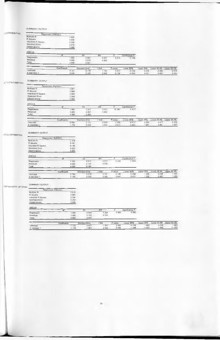
S U M M A R Y O U T P U T
E a i T i . t R egression StatisticsM u lt ip le R 0 8 0 5R S q u a r e 0 8 4 8A d ju s t e d R S q u a r e 0 5 3 0S t a n d a r d E r r o r 0 0 7 0O b s e r v a t i o n s 5 0 0 0
4 0 V A
df ss M SR e g r e s s io n 1 0 0 0 0 0 2 7 0 0 2 7 5 5 1 5 0 1 0 0R e s id u a l 3 0 0 0 0 0 1 5 0 0 0 5' o t a i 4 0 0 0 0 041
C o e ffic ie n ts Standard E rro r t Slat P -value Low er 9 5 % U p p e r 9 5 % Lo w e r 95 0%in t e r c e p t 0 141 0 11 8 1 19 7 0 3 1 7 •0 2 3 4 0 5 1 6 •0 234 0 5 1 6X V a r a o i e 1 0 2 3 4 0 1 0 0 2 3 4 8 0 1 0 0 •0 0 8 3 0 551 -0 08 3 0 551
3'T|*FA.EBrrcb)> S U M M A R Y O U T P U T
R egression StatisticsM u lt ip le R 0 941
R S q u a r e 0 8 8 6
A d j u s t e d R S q u a r e 0 8 4 8
S t a n d a r d E r r o r 0 0 4 9
O b s e r v a t i o n s 5 0 0 0
A N O V A
df S S M S F Significance FR e g r e s s i o n 1 0 0 0 0 0 5 7 0 0 5 7 2 3 3 6 7 0 0 1 7
R e s id u a l 3 0 0 0 0 0 0 7 0 0 0 2
T o t a l 4 0 0 0 0 0 6 4
C o e ffic ie n ts Standard Error t Stat P v a lu e L o w e r 9 5 % Upper 95% L o w e r 95 0 % U p p e r 95 0 %In te r c e p t -0 0 94 0 101 *0 9 2 8 0 4 2 2 - 0 4 1 7 0 2 2 9 • 0 4 1 7 0 2 2 9
X V a r ia b le 1 1 .1 7 4 0 2 4 3 4 8 3 4 0 0 1 7 0 4 0 1 1 9 47 0 401 1 9 4 7
S U M M A R Y O U T P U T3Tr>>.0=»*£3lTtb»R e g r e s s io n Statistics
M u lt ip le R 0 3 1 8
R S q u a r e 0 101
A d ju s t e d R S q u a re -0 198
S t a n d a r d E rro r 0 2 2 3
O b s e r v a t io n s 5 0 0 0
A N O V A
df S S M S F Significance FR e g r e s s io n 1 .0 0 0 0 .0 1 7 0 .0 1 7 0 3 3 9 0 6 0 2
R e s id u a l 3 0 0 0 0 1 49 0 0 5 0
T o t a l 4 0 0 0 0 1 66
Coefficients Standard Error t Stat P -valu e L o w e r 9 5 % Upper 95% Lo w e r 95 0% U p p e r 9 5 0 %
In te rc e p t 0 7 9 3 0 3 7 8 2 101 0 126 -0 4 0 8 1 9 9 5 -0 40 8 1 9 9 5
X V a r ia b le 1 0 18 6 0 3 2 0 0 5 8 2 0 6 0 2 - 0 83 1 1 2 0 3 -0 831 1 2 0 3
S U M M A R Y O U T P U T - 3 r T f c * o C f V T o p E X ^ b ) ] ____________________________
R e gressio n StatisticsM u ltip le R 0 8 1 6
R S q u a r e 0 6 6 5
A d ju s t e d R S q u a r e 0 55 4
S ta n d a r d E rro r 0 2 3 3
O b s e rv a t io n s 5 0 0 0
A N O V A
df S S M S F S K n fic a n c e F
R e g re s s io n 1 0 0 0 0 3 2 4 0 324 5 9 6 3 0 0 9 2
R e s id u a l 3 0 0 0 0 1 6 3 0 054
T o t a l 4 0 0 0 0 4 8 7
Coefficients Standard E m * r Stef P in k ie L o n e r 05 % U pf* * 05% L o w e r 9 5 0% U p p e r 9 5 0 %
in te rc e p t -1 1 8 3 0 9 5 7
X V a n a b le 1 4 7 7 8 1 9 5 7
-1 2 3 7 0 304
2 4 4 2 0 0 92
-4 2 2 8
• 1 .4 4 9
1 8 6 21 1 0 0 5
•4 2 2 8 • 1 4 4 9
1 6 6 2
1 1 .0 0 5
■

8
n
ss
o u*
31
85
o t*
3 ! *
|M M W
8§S
i
\

S3
o o— K) cr> -4
c, 63s
i§
i i *
SS
h a j )
*
»• w -*
§ § §
a
0.037 0 129 0 166
a
0 037 0 043
-n
i
o ■
T)
i l l ' c
%Jj
sm o o o
§ 2 § k
3t-3
- 6is
5?
i b
sg?
-1 7 ) JO
■ I f
f g§
o o28<0 - J
ffff• .0
» o o p
§sss§ sa
28
s£
2
o
25
25
£52
8S
if]
o o o o
Ig sss

soiisije
is uoiss
ajtetl

I

!
!
<ra)
x3 d
c

WO
O
6CI
O'
860
0 6C
I 0*
61
9 0
CSS
O'
ICO
0
120
O’
l W
MA
XS2
CI_
____
____
199
0___
____
_SZ
C I_
____
___
189
0___
____
___Z
00 0
____
____
KO
Ot_
____
____
_001
0__
____
____
900
t___
____
____
____
____
____
____
____
__|d
eo»M
%0 96
Mdd
n %
OS6
^o
t %
56 >
*ddn
%S6 '
WQ
l on
ie*-d
ie% i
iou3
pjvf
xvis_
____
____
s/tA
K^a
op__
____
____
____
____
____
____
__
tog
stm
s

s s s s i
g s s5 *- o
vt
g S r° 9
.■fS 2tn o
— o
*
s
I
S rc ° o o
i
.
I
isN
U.o o
a
2 2 | e
r
i n ;
0 14
5 0
046
a
1 00
0 30
00
4000 5 5
o o
111 fi
iiiio o o o *
0r
g5sss
o o5gS£Si9 9
3
£5so.io o
«sI*s
1o 9 9
3s3
%IfU. 1ci.|1 057 ! 194to5 So> tn O N «o o 5 6S3o o o o ototo
1 000
3 000
4000 1
0 130
0359
or <r °
i
} !
____
____
____
____
____
____
____
____
____
____
_C
oe
ffo
en
ts__
____
____
___
Sta
nd
ard
Err
or
t S
tat_
____
____
___
P-v
a!u
e
Lo
we
r 9
5%
U
ppe
r 9
5*
L
ow
er
95
.0%
U
pp
er
95
0%
inte
rce
pt
0 8
92
0
11
2
7 9
87
0
00
4
0 5
36
1
24
7
0 5
36
1
24
7
X V
aria
ble
1___
____
____
____
____
____
____
____
_Q
05
2__
____
____
____
_C
03
5__
____
____
____
__-4
67__
____
___
C 23
9___
____
___
-C 0
60
____
____
___
0 16
3___
____
__-0
06
0__
____
____
___
0 1
63

OP
EX
(b»
SU
MM
AR
Y O
UT
PU
T
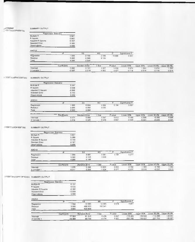
V
^ S U M M A R Y O U T P U T.9 TW)OpiaiT(i>)R e g r e s s io n S r a r s b c s
M u M X e R 0 92 1R S q u a re 0 8 4 7
A d ju s te d R S q u a r e 0 7 9 7
S ta n d a r d E rr o r 0 3 6 0
O b s e rv a t io n s 5 0 0 0
A N O V A
df s s M S Significance FR e g re s s io n i 0 0 0 2 1 6 0 2 160 16 6 6 6 0 0 2 7
R e s id u a l 3 0 0 0 0 3 8 9 0130T o t a l 4 0 0 0 2 5 4 9
Coefficients Standard E rro r t Slot P-vatue L o w e r 9 5 % U p p e r 9 5 % Lower 9 5 0 % « P P » » s 0 *in terce p t 0 6 8 3 0 191 3 56 7 0 0 3 8 0 0 7 4 1 2 9 2 0 0 7 4 1 2 9 2X V a ria b le 1 - 0 0 6 5 0 0 1 6 -4 0 8 2 0 0 2 7 - 0 1 1 6 •0 0 1 4 -0 1 1 6 -0 0 1 4
■' S * ~ ? - > H p A ~ E O T O ) ) ) S U M M A R Y O U T P U T
_________________R e g re ss ion StatisticsM u ltip le R
R S q u a re
A d ju s te d R S q u a r e
S ta n d a rd E r r o r
O b s e rv a t io n s ______________________________
A N O V A
df S S M S F Significance FR e g re s s io n 1 0 0 0 0 0 0 4 0 0 0 4 0 184 0 6 9 7
R e s id u a l 3 0 0 0 0 0 6 0 0 0 2 0
T o t a l 4 0 0 0 0 0 6 4
Coefficients Standard E rro r t S t at P-value L o w e r 9 5 % U p p e r 9 5 % Lower 9 5 0 % U p p e r 9 5 0 %
In te rce pt 0 .3 7 5 0 0 6 8 5 54 7 0 0 1 2 0 1 6 0 0 5 8 9 0 1 6 0 0 5 8 9
X V a n a b ie 1 0 0 3 8 0 0 8 9 0 4 2 9 0 6 9 7 -0 2 4 5 0 3 2 1 •0 2 4 5 0 3 2 1
£BT:ro;OPrtBT(t>» SUMMARY OUTPUT
0 24 1
0 0 5 8
-0 2 5 6
0 1 4 2
5 0 0 0
R e g re s s io n StatisticsM u ltip le R 0 6 0 7
R S q u a re 0 3 6 9
A d ju s te d R S q u a r e 0 1 5 9
S ta n d a rd E rr o r 0 18 7
O b s e rv a t io n s 5 0 0 0
A N O V A
df S S M S F Significance F
R e g re s s io n 1 0 0 0 0 06 1 0 061 1 7 5 4 0 2 7 7
R e s id u a l 3 0 0 0 0 10 5 0 0 3 5
T o t a l 4 0 0 0 0 1 6 6
Coefficients Standard Erro r t Stat P-vatue L o w e r 9 5 % U p p e r 9 5 % Lower 9 5 0 % U p p e r 9 5 0 %
Intercept 1 .0 7 8 0 0 9 9 10 8 3 5 0 0 0 2 0 7 6 0 1 3 9 3 0 7 6 0 1 39 3
X V a n a b ie 1 - 0 011 0 0 0 8 •1 3 2 4 0 .2 7 7 - 0 0 3 7 0 0 1 5 -0 0 3 7 0 0 1 5
E B r . ] b ; . y < O P i T O P E X ( b ) ) S U M M A R Y O U T P U T
R e gre s s io n StatisticsM u ltip le R 0 15 7
R S q u a re 0 0 2 5
A d ju s te d R S q u a r e •0 3 0 0
S ta n d a rd E rr o r 12 8 5 8
O b s e rv a t io n s 5 0 0 0
A N O V A
df S S MS F S ig n if ic a n c e F
R e g re s s io n 1 0 0 0 1 2 .5 8 5 12 58 5 0 0 7 6 0 801
R e s d o a i 3 0 0 0 4 9 6 0 2 3 165 341
T o ta l 4 0 0 0 5 0 8 6 0 8
Coefficients Standard Erro r t Stat P-vatue L o w e c 9 5 * U p p e r 9 5 % Lower 9 5 0 % Upper 9 S O %
intercept 1 7 82 4 4 1 5 1 5 0 4 2 9 0 6 9 7 -1 1 4 2 9 5 1 4 9 9 4 4 -1 1 4 2 9 5 1 4 9 944
X v a n a b ie 1 •18 9 6 8 6 8 7 5 0 ■0276 0 801 -2 3 7 7 6 2 1 9 9 8 2 7 -2 3 7 7 6 2 1 9 9 8 27

s
I
*5 | S 8 S S
5535
1s
uo
ets
aj&
9H

_________________________________________Co
efficie
nts____________
Sta
nd
ard
Erra
t I Slat_____________P
t/aiue
low
er 9
5%
u
pp
er 9
5%
lo
we
r 85
0*
U
pp
er tS
O%
Inte
rcep
t 1 0
76
0
09
9
10
83
5
0 0
02
0
76
0
1 3
93
0
76
0
1 39
3
X V
eu
ole
-1_________________________________________.0
011_______________0
00
5______________
-1 32a___________
02
77
______________0 037
____________0
015__________
-0 0
37
_____________0015
"r$
g
A W -
§§§
o o o
f i l l ?f
i f f»
1 !I
I
o o o o8 » 5 SS -4 IO « §

r § a 5 §
ise
§11
8229 9
S3
B 5
I S
i
§«- = §o o o o
III
§15
11§
i «K i t h
SI
go
2 £
«§2S§o o o c
r- CMo o o o
is?o o o
§11
Inte
rce
pt
1.1
32
0
28
8
3 9
31
0
02
9
0 2
15
2
04
8
0 2
15
2
04
8
X W
as
te 1
____
____
____
____
____
____
____
____
____
____
_-0
.03
6__
____
____
____
_0
07
8__
____
____
____
__04
69__
____
___
C67
J___
____
____
___
0 2
83
____
____
____
0 2
10
____
____
___
-0 2
83
____
____
____
02
10

o*»
ex<D
)j
SgSllO O 9 •- K>
I1
I
s
Io
86
ssso w »
111
esssss
SR
?»
*1!-s sI
S
8*
;s
3S
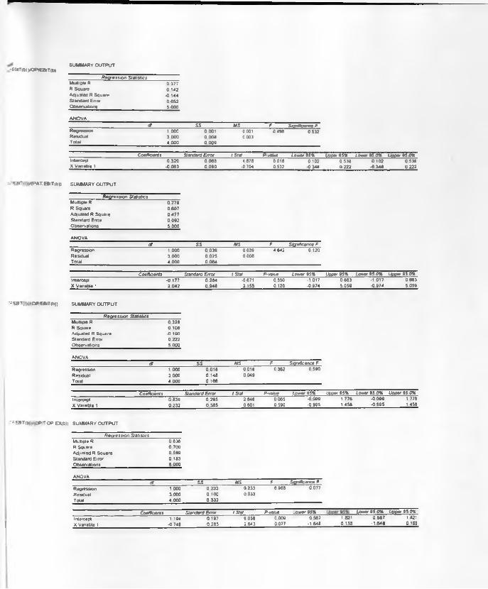
-snbi>op«iT(b) S U M M A R Y O U T P U T
R e p re s s* * ) StatisticsM u ltip le R 0 3 7 7R S q u a r e 0 14 2A d ju s t e d R S q u a r e •0 14 4S ta n d a r d E rr o r 0 0 5 2O b s e rv a t io n s 5 0 0 0
A N O V A
Of s s M S F S o n l lc t n c t FR e g re s s io n 1 0 0 0 0 00 1 0 001 0 4 9 6 0 5 3 2R e s id u a l 3 0 0 0 0 0 0 8 0 00 3T o t a l 4 0 0 0 0 0 0 9
Coefficients Standard E rro r I S I X P v U u t Lo w er 9 5 % U p p e r 9 5 % Lowe/ 95 0 % U pp e r 9 5 0 %in te rc e p t 0 3 2 0 0 0 6 8 4 6 7 8 0 0 1 8 0 1 0 2 0 5 3 8 0 1 0 2 0 53 8X V a r ia b le 1 •0 0 6 3 0 0 9 0 -0 7 0 4 0 5 32 •0 3 46 0 2 2 2 -0 3 4 0 0 2 2 2
: e = r . iS P A J . E B i T i b ) j S U M M A R Y O U T P U T
R e g r e s s i o n StatisticsM u ltip le R 0 7 7 9
R S q u a r e 0 6 0 7
A d ju s t e d R S q u a r e 0 4 7 7
S ta n d a r d E rr o r 0 0 9 2
O b s e r v a t io n s 5 0 0 0
A N O V A
df S S M S F Sksuficance FR e g re s s io n 1 0 0 0 0 0 3 9 0 0 3 9 4 6 4 2 0 1 2 0
R e s id u a l 3 0 0 0 0 0 2 5 0 0 0 8
T o t a l 4 0 0 0 0 0 6 4
Coefficients Standard E rro r t Slat P-value Lo w er 9 5 % U p p e r 9 5 % Lower 9 5 0 % U pp e r 95 0 %
in te rc e p t - 0 1 7 7 0 2 6 4 -0 671 0 55 0 -1 0 1 7 0 6 6 3 -1 .0 1 7 0 6 6 3
X V a ria b le 1 2 0 4 2 0 9 4 8 2 1 5 5 0 120 -0 9 7 4 5 0 5 9 - 0 9 7 4 5 0 5 9
: s « B T ; i . O P 'E B I T ( b ) ) S U M M A R Y O U T P U T
R e p re s sio n StatisticsM u ltip le R 0 3 2 8
R S q u a re 0 1 08
Ad|us**d R S q u a r e - 0 1 9 0
S ta n d a r d E rr o r 0 2 2 2
O b s e rv a t io n s 5 0 0 0
A N O V A
df S S M S F Significance F
R e g re s s io n 1 0 0 0 0 0 1 8 0 0 1 6 0 .3 6 2 0 5 9 0
R e s id u a l 3 0 0 0 0 .1 4 8 0 0 4 9
T o t a l 4 0 0 0 0 .1 6 6
Coefficients Standard Erro r f S ta r P-vatue L o w e r 9 5 % Upper 9 5 % Lower 9 5 0 % U p p e r 95 0%
in te rc e p t 0 8 3 9 0 2 9 5 2 8 4 6 0 0 6 5 -0 0 9 9 1 7 7 6 - 0 0 9 9 1 77 6
X V a ria b le 1 0 2 3 2 0 3 8 5 0 60 1 0 59 0 •0.995 1 4 5 8 - 0 9 9 5 1 4 58
I ; E 3 T | « . D P - O P E X ( b ) ) S U M M A R Y O U T P U T
R e g re s s io n StatisticsM u lt o le R 0 8 3 6
R S q u a re 0 7 0 0
A d ju s te d R S q u a r e 0 5 9 9
S ta n d a rd E r r o r 0 183
O b s e rv a t io n s 5 0 0 0
A N O V A
df S S M S F Significance F
R e g re s s io n 1 0 0 0 0 2 3 3 0 2 3 3 6 9 8 8 0 0 7 7
R e s rfu a i 3 0 0 0 0 .1 0 0 0 .0 3 3
T o t a l 4 0 0 0 0 3 3 3
Coefficients Standard Error r Slat P -valuc _ o w e r 9 5 % Lower 9 5 0 % Upper 95 0%
In te rce pt 1 194 0 1 97 8 0 5 8 0 0 0 9 0 5 6 7 1 82 1 0 5 8 7 1 821
X V e n a b le 1 - 0 7 4 8 0 2 8 3 •2 6 4 3 0 0 7 7 -1 6 4 8 0 15 3 • 1 .6 4 8 0 153

.'9*1
1
S3o o
C. r--
SI9
3 8
S 3
8*5
S 3
#:f .- CN: ? 9
, i i!°°
S3
(x;
IS3SJ o o
*5* f•- o
.3SJ o o
,ss
I I
§:::
§
►-8

(Mxado
'

.-6S’rt*yOP*CBrr(t>) S U M M A R Y O U T P U T
R e gressio n S ta tu te sM u lt ip le R 0 70 4
R S q u a r e 0 4 9 6A d ju s t e d R S q u a r e 0 3 2 8S t a n d a r d E rr o r 0 09 1
O b s e r v a t io n s 5 0 0 0
A N Q V A
df s s M S F S ig n if ic a n c e FR e g re s s io n 1 0 0 0 0 0 2 4 0 02 4 2 9 5 2 0 184R e s i d u a 3 0 0 0 0 0 2 5 0 0 0 8T o t a l 4 0 0 0 0 0 4 9
Coe fficie n t* Standard Erro r 1 Stat Pw alue l o w e r 9 5 % Upper 95% U p p « 9 ‘ 0 %in t e r c e p t
X V a r ia b le 1
-0 0 5 2 0 2 0 0
0 2 9 5 0 1 7 2
•0 2 6 0 0 8 1 2
1 7 1 8 0 184
0 6 8 8
•0 25 1
0 5 8 4
0 84 1
-0 6 8 8 0 5 8 4
-0 2 5 1 0 841
£ B T . T » » ^ » A r t B l T ( b ) ) S U M M A R Y O U T P U T
M u lt ip le R 0 6 8 7
R S q u a r e 0 4 7 2
A d ju s t e d R S q u a r e 0 2 9 6
S t a n d a r d E rr o r 0 10 6
O b s e r v a t io n s 5 0 0 0
A N O V A
dt S S M S F S ig n if ic a n c e FR e g re s s io n 1 0 0 0 0 0 3 0 0 0 3 0 2 6 6 2 0 2 0 0
R e s o u a i 3 0 0 0 0 0 3 4 0 0 1 1
T o t a l 4 0 0 0 0 0 6 4
C o e ffln e n ls Standard E rro r t Stat P -value l o w e r 9 5 % U p p a rtS X Low er 95 0 % Upper 95 0 %In te rc e p t 0 1 6 2 0 1 44 1 121 0 344 -0 2 9 7 0 6 2 0 •0 2 9 7 0 6 2 0
X V a r ia b le 1 0 7 8 5 0 .4 7 9 1 6 3 8 0 20 0 -0 7 4 0 2 3 1 0 -0 7 4 0 2 3 1 0
: f r £ r - I I > ; ^ D P € B l T ( b ) > S U M M A R Y o u t p u t
R e gres s io n StatisticsM u ltip le R 0 4 7 9
R S q u a r e 0 2 2 9
A d ju s t e d R S q u a r e •O 0 2 8
S ta n d a r d E r r o r 0 2 0 7
O b s e r v a t io n s 5 0 0 0
A N Q V A
dt S S M S F S ig n if ic a n c e F
R e g re s s io n 1 0 0 0 0 0 3 8 0 0 3 8 0 8 9 3 0 4 1 4
R e s id u a l 3 0 0 0 0 .1 2 8 0 0 43
T o t a l 4 0 0 0 0 1 6 6
Coefficients Standard Erro r t Stat P -value l o w e r 9 5 % Upper 95 % Lower 9 5 0 % U pp e r 95 0 %
in te rc e p t
X V a r ia b le 1
0 5 8 5 0 4 5 4
0 3 6 9 0 3 9 0
1 2 8 8 0 28 8
0 9 4 5 0 4 1 4
•0 8 6 0
- 0 8 7 4
2 0 3 0
1 61 1
-0 8 6 0
-0 8 7 4
2 0 3 0
1 61 1
O T ' t l k V Q P / T O P E X ( b ) ) S U M M A R Y O U T P U T
R e gre s s io n StatisticsM u ltip le R 0 0 0 4
R S q u a re 0 0 0 0
A d ju s t e d R S q u a r e 0 3 3 3
S ta n d a r d E rr o r 0 3 0 5
O b s e rv a t io n s 5 0 0 0
A N Q V A
dt S S M S F Significance F
R e g re s s io n 1 0 0 0 0 0 0 0 0 0 0 0 0 0 0 0 0 9 9 5
R e s id u a l 3 0 0 0 0 2 8 0 0 0 9 3
T o t a l 4 0 0 0 0 2 8 0
Coefficients Standard E rro r t Stat P-value Lo w e r 95% Lift* . 9 5 % lo w e r 9 5 0 % U p p a .9 5 0 %
in te rc e p t
X V a ria b le 1
1 1 3 3
0 0 1 3
0 8 7 2
1 9 2 4
1 3 0 0 0 2 8 5
0 0 0 7 0 9 9 5
-1 641
•6 10 9
3 9 0 7
6 1 3 6
-1 6 4 1
-6 1 0 9
3 90 7
6 136

I
*558-°IS? *? -
o o 5
§11*- r> v
* S Ia o » -
1* 5>?s 9 9
I
s S Io —
i
§s :9 9
!55
io o
Q
s 'i
?
1 I so o
4
i
0 1
84
0 7
25
a | ?£I S
8 5 ?
N f i o i m o
S S K K 8
t i l li f l i i
i i i
a a h
\
?-
____
____
____
____
____
____
____
____
____
____
_C
oeff
icie
nts_
____
____
____
sta
nd
ard
Err
or
I S
tat_
____
____
___
P v
alue
L
on
er
95
%
Upp
e,
95
%
Lorr
tr 9
5 0
%
Up
pe
r 9
5 0
%
Inte
rce
pt
0 9
60
0
46
8
2 0
49
0
.13
3
0 5
31
2
45
1
-0 5
31
2
.45
1
X V
an
**
; 1_
____
____
____
____
____
____
____
____
____
____
_0
06
6__
____
____
____
_0
66
0__
____
____
____
_0
IOC
0
92
7__
____
____
___-
2 0
34
2
1
65
2
03
4__
____
____
____
2 1
65

SfT
*|
MO
CT
OP
EX
<t»)

P
* b
2 6
87
50
68 1
o bS
SI•o
o o 1s s
I— 6*
S 3s
I»
w* o o o o
SSS i s
0
8
1
ls*•s SS
!Y O
UT
PU
T

_________________________________________Coefficients_____________S
tan
da
rd E
rror
t Sla
t____________P-va
fire
Lo
ne
r 95
*
Upper 9
5%
Lo
we
r 95
0%
u
pp
er 9
5 0
%in
terc
ep
t 1
21
9
0 4
07
2
99
3
0.0
58
-0
07
7
2 5
16
-0
07
7
2 5
16
X V
en
ab
le I__________________________________________0
10
5_______________
0 1
93
________________0 5
<2
___________0
62
5_____________
-0 7
16
____________0
50
9___________-0
71
6_____________0
50
9
§ i § I S ; I s
o o o
I
i
r
0<
j ?
s
l

f —
« * ■ * S U M M A R Y O U T P U T
. Regressio n Sta tisticTU u f t i p t e R 0 9 1 4
R S q u a r e 0 8 3 5
A d ju s t e d R S q u a r e 0 7 8 0S ta n d a r d E rro r 0 1 06
O b s e rv a t io n s 5 0 0 0
A N O V A
d T ss M S F Significance FR e g re s s io n 1 0 0 0 0 1 6 9 0 169 1 5 151 0 0 3 0R e s id u a l 3 0 0 0 0 0 3 4 0 0 1 1T o t a l 4 0 0 0 0 2 0 3
C o e ffic ie n ts Standard Error f Star R value l o w e r 9 5 % Upper 9 5 % L o v m 9 5 0 * U p p e r 9 5 0 %in te r c e p t 0 23 1 0 0 7 0 3 3 30 0 04 5 0 0 1 0 0 4 5 3 0 0 1 0 0 4 5 3X v a r ia b le 1 - 0 1 3 3 0 0 3 4 -3 8 92 0 0 3 0 - 0 2 4 2 -0 0 2 4 •0 2 4 2 -0 0 2 4
S U M M A R Y O U T P U T*-5 * T '7 1 P ^ * A '' £ B S T ( 5 ) ) _______________________________________
____________________R e gression St*M u ltip le R 0 3 9 0
R S q u a r e 0 1 5 2
A d ju s t e d R S q u a r e -0 .1 3 0
S t a n d a r d E rr o r 0 1 3 5
O b s e rv a t io n s _______________________________________________5 OOP
A N O V A
df S S M S F Significance FR e g re s s io n 1 0 0 0 0 0 1 0 0 0 10 0 5 4 0 0 5 1 6
R e s id u a l 3 0 0 0 0 0 5 4 0 018
T o t a l 4 0 0 0 0 0 6 4
C o e ffic ie n ts Standard Erro r t S ta r P -v a lu e l o w e r 9 5 % Upper 95% L o w e r 95 0 % U p p e r 95 0 %
In te rc e p t 0 3 9 2 0 06 1 6 42 5 0 0 08 0 198 0 5 86 0 19 8 0 5 8 6
X V a n a b le 1 -0 2 1 9 0 2 9 9 -0 735 0 5 16 -1 17 0 0 731 -1 17 0 0 731
S U M M A R Y O U T P U TT3.-::o:opr®mt») _________R e gres s io n Statistics
M u lt ip le R 0 .2 0 1
R S q u a r e 0 0 4 0
A d ju s t e d R S q u a r e -0 2 8 0
S ta n d a r d E rr o r 0 2 3 0
O b s e r v a t io n s 5 0 0 0
A N O V A
df S S M S F Significance FR e g re s s io n 1 0 0 0 0 0 0 7 0 007 0 12 6 0 7 4 6
R e s id u a l 3 0 0 0 0 1 5 9 0 053
T o t a l 4 0 0 0 0 1 6 6
C o e ffic ie n ts Standard Erro r f Slat P -value L o w e r 9 5 % Upper 95% Lo w er 95 0 % u p p e r > S 0 %in te rc e p t 0 9 6 6 0 151 6 37 6 0 0 0 8 0 4 8 4 1 4 4 8 0 4 8 4 1 4 4 8
X V a r ia b le 1 0 0 2 6 0 0 7 5 0 3 5 5 0 746 - 0 211 0 2 6 4 -0 2 1 1 0 2 6 4
r a r r « i * o P f T o p E x < t > »
S U M M A R Y O U T P U T
! |
M u ltip le R 0 3 6 9
R S q u a r e 0 1 3 7
A d ju s t e d R S q u a r e -0 151
S ta n d a r d E rro r 1 6 5 7
O b s e rv a t io n s 5 0 0 0
A N O V A
df S S M S F Significance F
R e g re s s io n 1 0 0 0 1 .3 0 3 1 303 0 4 7 4 0 5 4 0
R e s id u a l 3 0 0 0 8 2 4 1 2 747
T o t a l 4 0 0 0 9 5 4 4
Coefficients Standard Erro r t Stat P -value l o w e r 9 5 % U p p e r 9 5 % Low er 9 5 0 % U p p e r 95 0 %
in te rc e p t 0 1 0 2 2 .1 4 4 0 04 6 0 96 5 - 6 721 6 92 6 •6 721 6 9 2 6
X V e n a b le 1 2 5 6 9 3 .7 3 0 0 6 8 9 0 54 0 - 9 3 0 3 14 441 -9 3 0 3 14 44 1

s ;s§ §o o o o m
5
gSS
m9 9
51
§5o o
SS
§r*
s i
§2
Is9 9
§S
SS
8 o
____
____
____
____
____
____
____
____
____
____
Coe
ffic
ient
s___
____
____
__S
tand
ard
Err
or_
____
____
_t
Sta
l___
____
____
_P-t
ram
e
Lo
we
r 9
5%
U
ppe
r 9
5%
Lo
we
r 9
5 0
%
Up
pe
r 9
5 0
Xin
terc
ep
t 0
88
3
0 3
44
2
57
0
0 0
82
-0
21
0
1 9
77
-0
21
0
1 9
77
X V
ar-
aW
__
____
____
____
____
____
____
____
____
____
____
C 1
04
____
____
____
___0
28
C__
____
____
____
__I
27
3__
____
____
__3
734_
____
____
____
0 7
87
____
____
____
_G
9%
____
____
___
C 7
87
____
____
____
_0
99
6

7*
mm
*P
PtT
op
ex
o»
)
v*

—
S U M M A R Y O U T P U T
M k O P ' t i T w R e g r e s s io n S /ar.sr*ci
M u m p * R 0 5 9 2R S q u a r e 0 3 5 0A O ju s t e d R S q u a r e 0 1 3 3S t a n d a r d E n o r 0 0 3 4
O b s e r v a t io n s 5 0 0 0
> N Q V A
d 1 s s M S F S o M I c a m fR e g r e s s io n 1 000 0 002 0 002 1 615 0 293R e s a J u a i 3 0 0 0 0 003 0 001T o t a l 4 000 0 005
Coefficients Standard Error 1 S (* P -r t t k * Lo w er 9 5 % U p p e r 9 5 % L o w e r 9 5 O X U p p e r 9 5 0%in t e r c e p t 0 1 23 0 0 5 0 2 4 7 3 0 0 90 •0 0 3 5 0 281 •0 0 3 5 0 281
X V a r ia b le 1 -0 0 4 7 0 0 3 7 •1 2 71 0 2 93 •0 16 6 0 0 7 1 -0 166 0 07 1
r3*jrkypATraT(b): S U M M A R Y O U T P U T
R e gressio n S ta tiU < sM u lt ip le R 0 1 5 0
R S q u a r e 0 0 2 2
A d j u s t e d R S q u a r e -0 30 4
S t a n d a r d E rro r 0 144
O b s e r v a t io n s 5 0 0 0
A N O V A
d f S S M S F Significance FR e g r e s s io n 1 0 0 0 0 0 0 1 0 0 0 1 0 0 6 9 0 8 1 0
R e s id u a l 3 0 0 0 0 0 6 3 0 021
T o t a l 4 0 0 0 0 0 6 4
C o e ffic ie n ts Standard Error t Stat P value L o w e r 9 5 % U p p e r 9 5 % Lo w e r 9 5 0 % U p p e r 9 5 O X
in t e r c e p t 0 4 1 7 0 141 2 95 9 0 06 0 -0 0 3 2 0 8 6 6 -0 0 3 2 0 8 6 6
X V a r ia b le 1 -0 5 2 4 2 0 0 2 - 0 26 2 0 8 1 0 -6 8 9 5 5 84 6 •6 8 9 5 5 6 4 6
S U M M A R Y O U T P U T
R e gres s io n StatisticsM u lt ip le R 0 351
R S q u a r e 0 1 23
A d j u s t e d R S q u a r e -0 1 69
S t a n d a r d E rr o r 0 2 2 0
O b s e r v a t io n s 5 0 0 0
A N O V A
d f S S M S F Significance F
R e g r e s s io n 1 0 0 0 0 0 2 0 0 020 0 421 0 5 6 3
R e s id u a l 3 0 0 0 0 1 4 6 0 049
T o t a l 4 0 0 0 0 1 6 6
C o e ffic ie n ts Standard Error 1 Stat P - value L o w e r 9 5 % U p p e r 9 5 % Lower 9 5 0 % U p p e r 95 0 %
in t e r c e p t 1 2 0 7 0 3 2 6 3 7 0 7 0 03 4 0 171 2 2 4 2 0 .1 7 1 2 2 4 2
X V a r ia b le i - 0 159 0 2 4 5 -0 6 49 0 5 6 3 •0 9 3 9 0 62 1 -0 9 3 9 0 6 21
O P E X ( b »
S U M M A R Y O U T P U T
____________________ R e gressio n StatisticsM u lt ip le R
R S q u a r e
A d ju s t e d R S q u a r e
S t a n d a r d E r r o r
O b s e r v a t io n s ______________________________
0 7 4 9
0 561
0 4 1 5
0 3 4 4
5 0 0 0
A N O V A
df S S M S F Significance F
R e g re s s io n 1 0 0 0 0 4 5 4 0 454 3 8 3 6 0 145
R e s id u a l 3 0 0 0 0 3 5 5 0 1 1 8
T o t a l 4 0 0 0 0 8 0 9
C o e fficients Standard Error t Stat P -vakie L o w e r 9 5 % Upper 95 % Lo w er 95 0 % U pp e r 95 0 %
in te rc e p t • 1 9 4 9 1 6 4 9 -1 182 0 3 2 2 - 7 197 3 2 9 9 •7 1 9 7 3 2 9 9
6 4 0 4 3 2 7 0 1 9 5 8 0 145 •4 0 0 2 16 8 0 9 -4 0 0 2 1 6 8 0 9

g
x 5 < 5
i j
fo O
M £
I
0 7
22
1 47
4
I
?
- 6 8
5 §
7>
o o !S s
1NJ
S t<£> -Js
!2 149 6 833 $
1f\J fo SS £ S
fot N) 5
2 1 3
Regression Statutes

Re
gn
ivo
n S
tatistic i

r"
8
Is
6 o
8§
3s
§S
8SB»
- i JJ X
I I !
ill
-4 - J O8 5 S
3 - "
<2 £ » fa a c -g.
s i r
in o 6 O o
is S Is
SU
MM
AR
Y O
UT
PU
T

i sI s
ss
o o ;
S 8
6 o '2 ® a
scS S *
6 o i
SS .cn M 0
ssi
H » »
t | f= «
§ § §
s5k
s s
* l |
l/i o o o o ss
o o P
.65is 8'
s i s
§§§
Isi
f l
1/ o o o o
i s s s s
r
I s
i t
§§§
O O Ib © ' cn *•
i l l
(/i o o o o
= 2iSSo, hJ <o - I
[Y OU
TPUT

«Q)X3
dO i/d
0M«l>
ll83'<
*O!

_______________________________________Co
efTa
en
ts_____________S
tan
da
rd E
rror_________t S
tat____________P-va
lue
Lo
we
r 95
%
Up
pe
r 95
%
Lo
we
r 95 0
%
Up
pe
r 95
0%
ln»e
fce
p«
0 8
85
0
27
0
3 2
81
0
0*
6
0 0
27
1 7
44
0
02
7
1 7
44
X V
aria
ble
1________________________________________0
09
8_______________
0 2
04
_______________0
48
0___________
0 6
64
_____________-0
S5
3____________0
74
9___________-0
55
3_____________0
74
9
m
i l l
o o o
8ES
o o8 2— N»
u< o 6 o o
i s
ss
§§§
o o o
?§§
o o
§5
s
I jif f !
v> o o o o
I S s f *
SS
i s
8 2
i § §
§SS
§§SS3
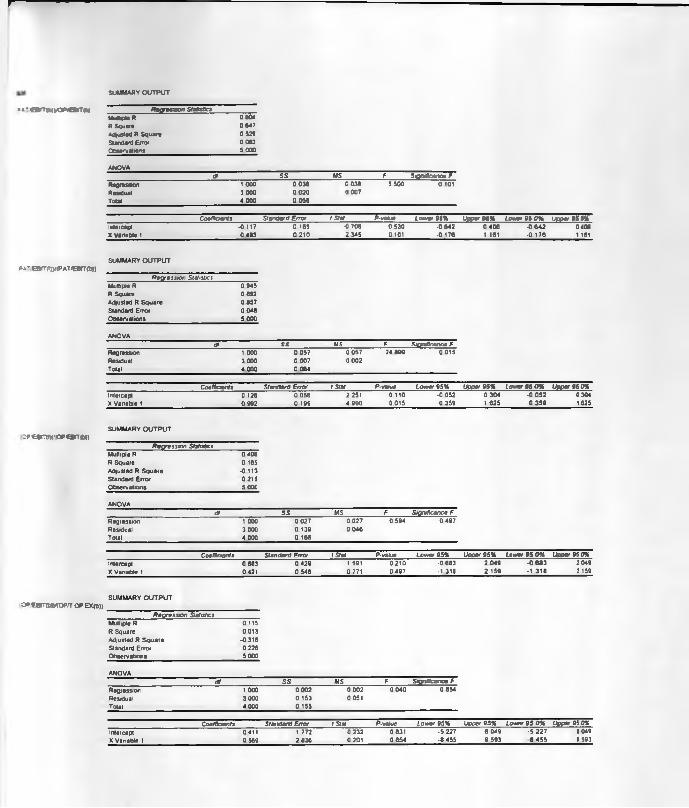
I
S U M M A R Y O U T P U T
*A-®rr«*DP€9iT<bj ____________Reanmen StmettcsU u M X t R 0 80 4
R S q u a re 0 6 4 7
A d ju ste d R S q u a r e 0 52 9
S ta n d a rd E rro r 0 0 8 3
O b s e rv a tio n s 5 0 0 0
A N O V A
Of s s M S F Significance FR e g re ss io n 0 0 0 0 0 3 8 0 0 3 8 5 5 0 0 0 101
R e s rfu a l 3 0 0 0 0 0 2 0 0 0 0 7
To ta l 4 0 0 0 0 0 5 8
Coefficients Standard Erro r tSta t P-value L o w e r 9 5 % upper M X Lo ne r » 5 O X Upper 9 5 0 *
intercept - 0 117 0 16 5 •0 7 0 8 0 5 3 0 -0 6 4 2 0 4 0 8 •0 6 4 2 0 4 0 8
X V a n a b te i 0 4 9 3 0 2 1 0 2 3 4 5 0 101 •0 17 6 1 161 •0 1 7 6 1 161
P i T € B T T ( I )V ( P A T € 8 r r < l » )
S U M M A R Y O U T P U T
R e gressio n StatisticsM u ltip le R 0 9 4 5
R S q u a re 0 8 92
A d ju s te d R S q u a r e 0 8 5 7
S ta n d a rd E rr o r 0 0 4 8
O O s e rv a tio n s 5 0 0 0
A N O V A
Of S S M S F S w f ic a n c e FR e g re s s io n 1 0 0 0 0 0 5 7 0 0 5 7 2 4 8 9 9 0 0 1 5
R e sid u a l 3 0 0 0 0 0 0 7 0 0 0 2
T o ta l 4 0 0 0 0 0 6 4
Coefficients Standard Erro r t Stat P -value L o w e r 95 % Upper 9 5 % Lower 9 S O % U pp e r 9 5 0 %in terce p t 0 126 0 0 5 6 2 2 5 1 0 11 0 -0 0 5 2 0 3 0 4 -0 0 5 2 0 304
X v a r ia b le 1 0 9 9 2 0 19 9 4 9 9 0 0 .0 1 5 0 3 5 9 1 6 2 5 0 3 5 9 1 6 2 5
S U M M A R Y O U T P U T
:P € B T [T K -? O P € B f T < b M ____________________________
R e gressio n StatisticsM u ltip le R 0 4 0 6
R S q u a re 0 165
A d ju s te d R S q u a r e - 0 1 1 3
S ta n d a rd E r r o r 0 21 5
O b s e rv a t io n s 5 00 0
A N O V A
at s s MS F Significance F
R e g re s s io n 1 00 0 0 0 2 7 0 0 2 7 0 5 9 4 0 4 9 7
R e s id u a l 3 0 0 0 0 139 0 0 4 6
T o ta l 4 00 0 0 166
Coefficients Standard Error tSta t P-value Lo w e r 95% Upper 9 5 % Lower 95 0 % Upper 95 0%
in terce p t 0 68 3 0 4 2 9 1 591 0 2 1 0 -0 6 8 3 2 0 4 9 •0 6 8 3 2 04 9
X V a ria b le 1 0 4 2 1 0 5 4 6 0 771 0 4 9 7 •1.318 2 .1 5 9 •1 3 1 8 2 159
C P€*T (W H O P.T OP EX(b»S U M M A R Y O U T P U T
R e g r e s s io n Statistics
M u ltip le R 0 1 1 5
R S q u a re 0 0 1 3
A d ju s te d R S q u a r e -0 3 1 6
S ta n d a rd E r r o r 0 2 26
O b s e rv a t io n s 5 0 0 0
A N O V A
df S S M S F Significance F
R e g re s s io n 1 o oo 0 0 0 2 0 0 0 2 0 0 4 0 0 8 5 4
R e s id u a l 3 0 0 0 0 153 0 05 1
T o ta l 4 00 0 0 155
Coefficients Sta ixta rd Error f Stat P -value Lo w er 95% U p p e r 9 5 % Low er 95 0 % Upper 95 0%
in terce p t 0 4 1 1 1 7 7 2 0 2 3 2 0 83 1 - 5 2 27 6 0 4 9 •5 2 2 7 5 04 9
X V a ria b le 1 0 56 9 2 8 3 6 0 2 0 1 0 8 5 4 •8 4 55 9 59 3 8 4 5 5 9 593

f
SUMMARY OUTPUT
-*’»«»vOP«rr<b> ______ffxwiwr StatutesM k A p t t R 0 351
R S q u a re 0 123
A d ju ste d R S q u a r e - 0 169
S ta n d a rd E rro r 0 0 3 4
O b s e rv a b o n s 5 0 0 0
A N O V A
df s s M S F S m f r a n c e FR e g re s s io n 1 0 0 0 0 0 0 0 0 0 0 0 0 42 1 0 5 6 3R e w Ju a r 3 0 0 0 0 0 0 3 0 001
T o ta l 4 0 0 0 0 0 0 4
Coefficient* Standard Erro r t Stat P -value L o w e r 9 5 % U u x r t S X Lower 9 5 0 % U pp e r 95 0%in tercept 0 151 0 1 4 6 1 0 3 8 0 3 7 5 -0 3 1 2 0 6 1 5 - 0 3 1 2 0 6 1 5X V e n a b le 1 0 172 0 2 6 6 0 6 4 9 0 56 3 -0 6 7 3 1 0 1 8 -0 6 7 3 1 0 1 8
S k 's r r c : .(PAT.€BrT(b))S U M M A R Y O U T P U T
R e g r e s s io n Stat e sM u ltip le R 0 196R S q u a re 0 0 3 8
A d ju s te d R S q u a r e - 0 2 8 2
S ta n d a rd E rro r 0 143O b s e rv a t io n s 5 0 0 0
A N O V A
df S S M S F S K jn.fr& nce FR e g re s s io n 1 .0 0 0 0 0 0 2 0 0 0 2 0 1 2 0 0 7 5 2
R e s id u a l 3 0 0 0 0 0 6 2 0 021T o ta l 4 0 0 0 0 0 6 4
Coefficients Standard Erro r t Stat P-vaiue L o w e r 9 5 % Lower 9 5 0 % Upper 9 5 0 %
in terce p t 0 191 0 561 0 34 1 0 75 6 •1 5 9 5 1 9 7 8 -1 5 9 5 1 97 8X V a n a t te 1 0 7 8 8 2 2 7 5 0 3 4 7 0 75 2 -6 451 8 0 2 8 -6 4 5 1 8 02 8
S U M M A R Y O U T P U Tz p a r r r»t > o p « a T o » ) ____________________________
R e g r e s s i o n StatisflcsM u ltip le R 0 3 4 3
R S q u a re 0 118
A d ju s te d R S q u a r e - 0 176
S ta n d a rd E rr o r 0 221
O b s e rv a t io n s 5 0 0 0
A N O V A
df S S M S F Significance FR e g re s s io n 1 0 0 0 0 0 2 0 0 0 2 0 0 4 0 0 0 5 7 2
R e s id u a l 3 0 0 0 0 14 6 0 0 4 9
T o ta l 4 0 0 0 0 1 6 6
Coefficients Standard Erro r t Stat P value L o w e r 9 5 % I Lower 9 5 0 % Upper 9 5 0 %
in terce p t 0 4 1 1 0 9 4 5 0 4 3 5 0 6 9 3 -2 .5 9 6 3 4 1 8 - 2 5 9 6 3 4 1 8
X v a n a b le 1 1 .0 9 0 1 7 2 3 0 6 3 3 0 5 7 2 -4 3 9 4 6 5 7 4 -4 3 9 4 6 574
O P€*T**|C W T OP EX(t»)S U M M A R Y O U T P U T
R e g r e s s i o n StatisticsM u ltip le R 0 .1 6 5
R S q u a re 0 0 2 7
A d ju s te d R S q u a r e -0 2 9 7
S ta n d a rd E rr o r 0 0 7 3
O b s e rv a t io n s 5 0 0 0
A N O V A
df S S M S F Significance FR e g re s s io n 1 0 0 0 0 0 0 0 0 0 0 0 0 0 8 4 0 79 1
R e s id u a l 3 0 0 0 0 0 1 6 0 0 0 5
T o ta l 4 0 0 0 0 0 1 6
Coefficients Standard E rro r t Stat P value Upper 95 % Lower 9 5 0 % U pp e r 95 0%in terce p t 0 39 9 0 5 0 7 0 7 8 5 0 49 0 -1 2 1 6 2 0 1 3 -1 2 1 6 2 01 3
X V a ria b le 1 0 2 6 0 0 8 9 8 0 2 9 0 0 791 -2 5 9 7 3 1 17 •2 5 9 7 3 117
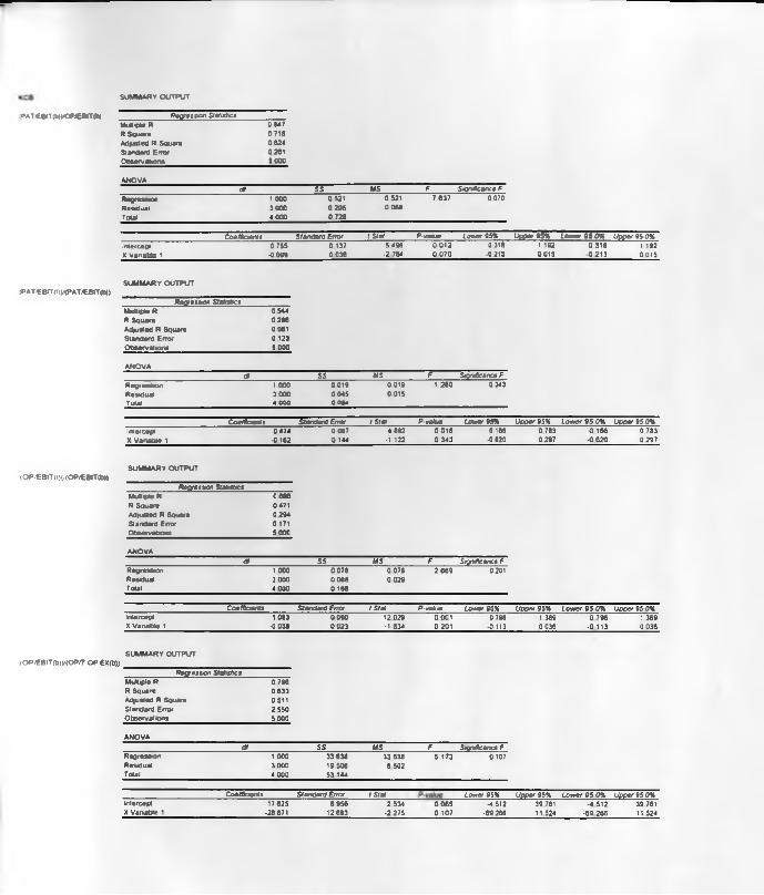
?AT€BlTH>»OP/€BfT<b)
SUMMAR Y OUTPUT
Regression StatisticsM u ltip le R 0 8 4 7
R S q u a r e 0 7 1 8
A d ju s te d R S q u a r e 0 6 2 4
S ta n d a r d E rr o r 0 261
O b s e r v a t io n s 5 0 0 0
A N O V A
df s s M S F Significance F
R e g re s s io n 1 0 0 0 0 521 0 521 7 6 3 7 0 07 0
R e s id u a l 3 0 0 0 0 2 0 5 0 0 6 8
T o ta l 4 0 0 0 0 72 6
C o e A fo e n f i Standard Error t Slat P -valu e L o n e r 9 5 % U p p e r 9 5 % L o w e r 9 5 0 % U pp e r 95 0 %in te rc e p t 0 7 5 5 0 1 3 7 5 4 9 6 0 0 1 2 0 318 1 192 0 3 1 8 1 192
X V a n a w e i ■0 0 9 9 0 0 3 6 -2 76 4 0 0 7 0 -0 2 1 3 0 0 1 5 - 0 2 1 3 0 0 1 5
(PAT€»T(I)yCPAT/€BIT(b))S U M M A R Y O U T P U T
Regression StatisticsM u ltip le R 0 54 4
R S q u a r e 0 2 9 6
A d ju s t e d R S q u a r e 0 061
S ta n d a r d E r r o r 0 123
O b s e r v a t io n s 5 0 0 0
A N O V A
dt S S M S F Significance FR e g r e s s io n 1 0 0 0 0 0 1 9 0 0 1 9 1 2 6 0 0 343
R e s id u a l 3 0 0 0 0 0 4 5 0 0 15
T o t a l 4 0 0 0 0 0 0 4
Coefficients Standard Error l Slat P -vaiu e Low er 9 5 % U pp e r 95% L o w e r 9 5 0 % U pp e r 9 5 0 %In te rc e p t 0 4 7 4 0 09 7 4 69 2 0 0 1 6 0 166 0 783 0 16 6 0 78 3
X V a r ia b le 1 -0 1 6 2 0 144 -1 122 0 3 4 3 -0 62 0 0 29 7 •0 6 2 0 0 2 9 7
S U M M A R Y O U T P U TtOf»BiTnH,(OP/EBrr(b)) _________Regression Statistics
M u ltip le R 0 6 8 6
R S q u a r e 0 471
A d ju s t e d R S q u a re 0 2 9 4
S ta n d a r d E rro r 0 171
O b s e rv a t io n s 5 0 0 0
A N O V A
df S S M S F Significance FR e g re s s io n 1 0 0 0 0 0 7 8 0 0 7 8 2 6 6 9 0 201
R e s id u a l 3 0 0 0 0 0 88 0 0 2 9
T o ta l 4 0 0 0 0 166
Coefficients Standard Error t Star P -vaiu e L o w e r 9 5 % Upper 95% L o w e r 9 5 0 % Upper 95 0 %In te rc e p t 1 0 8 3 0 0 9 0 12 0 2 9 0 0 0 1 0 796 1 369 0 7 9 6 1 3 6 9
X V a r ia b le 1 -0 0 3 8 0 0 2 3 • 1 6 3 4 0 2 0 1 -0 1 1 3 0 03 6 -0 .1 1 3 0 0 3 6
(O P T E B l T ( b ) V ( O P / T O P E X (b ) )
S U M M A R Y O U T P U T
____________________Regression StatisticsM u ltip le R
R S q u a r e
A d ju s t e d R S q u a r e
S ta n d a r d E r r o r
O b s e r v a t io n s _____________________________
0 7 9 6
0 6 3 3
0 511
2 5 5 0
5 0 0 0
A N O V A
df S S M S F Signtfcance FR e g re s s io n 1 0 0 0 3 3 6 3 8 3 3 6 3 8 5 1 7 3 0 1 0 7
R e s id u a l 3 0 0 0 19 50 6 6 502
T o t a l 4 0 0 0 5 3 144
Coefficients Standard Error_________ t Slat L o n e r 9 5 % U pper 95 % L o w e r 9 5 O X U pp e r 95 0 %
-4 5 1 2 3 9 761 -4 5 1 2 3 9 761
-6 9 26 6 11 52 4 -6 9 2 6 6 11 52 4
in te rc e p t
X V a r ia b le 1
17 6 2 5
•28 871
6 9 5 6
12 6 9 3
2 534
-2 2 7 5
0 0 6 5
0 1 0 7
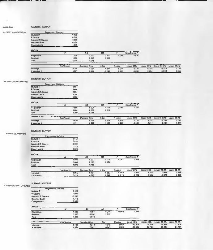
s a t orr (b)>OP€8rr <t»SUMMARY O U TPU T
R egression Statistics
M u A p t e R 0 136
R S q u a re 0 0 1 0
A d ju s te d R S q u a r e •0 30 6
S ta n d a rd E rr o r 0 07 0
O b s e rv a t io n s 5 0 0 0
A X O V A
at s s M S F S xjnAcance FR e g re s s io n 1 0 0 0 0 0 0 0 0 0 0 0 0 0 5 8 0 6 2 5
R e v d u a J 3 0 0 0 0 0 1 5 0 0 0 5
T o ta l 4 0 0 0 0 0 1 5
Coefficients S ta n dard Error tS ta t P-value L o w e r 9 5 % U p p e r 9 5 % L o w e r 9 5 0 % Upper 9 5 0 %
in terce p t 0 2 5 9 0 03 1 6 2 6 7 0 0 0 4 0 159 0 35 9 0 1 5 9 0 35 9
X v e n a b le 1 •0 0 0 7 0 0 2 9 -0 24 1 0 8 2 5 -0 0 96 0 0 64 •0 0 9 8 0 06 4
. P A T o r r ( n v ( P A T ' E B « T ( b ) )
S U M M A R Y O U T P U T
Regressio n Statistics
M u ltip le R 0 6 6 4
R S q u a re 0 4 4 0
A d ju s te d R S q u a r e 0 2 54
S ta n d a rd E r r o r 0 109
O b s e rv a t io n s 5 00 0
A N O V A
at s s M S F Significance FR e g re s s io n 1 00 0 0 0 2 6 0 0 2 8 2 3 6 0 0 22 2
R e s id u a l 3 00 0 0 0 3 6 0 0 1 2
T o ta l 4 0 0 0 0 0 0 4
Coefficients S ta n dard Error t Stat P -valu e L o w e r 9 5 % Upper 9 5 % Lo w er 9 5 0 % U p p a f 9 i0 %
in terce p t 0 0 2 9 0 2 3 6 0 1 2 5 0 9 0 9 -0 722 0 781 •0 7 2 2 0 781
X V a ria b le 1 1 371 0 8 9 2 1 5 3 6 0 2 2 2 -1 46 9 4 2 1 1 -1 4 6 9 4 211
S U M M A R Y O U T P U T<op«Brrcnwqp«T*i _________R e gressio n Statistics
M u ltip le R 0 142
R S q u a r e 0 02 0
A d ju s te d R S q u a r e •0 306
S ta n d a rd E r r o r 0 23 3
O b s e rv a t io n s 5 0 0 0
A N Q V A
Of S S M S F Significance F
R e g re s s io n 1 00 0 0 0 0 3 0 0 0 3 0 0 6 2 0 81 9
R e s id u a l 3 00 0 0 16 3 0 0 5 4
T o u t 4 00 0 0 16 6
Coefficients Sta n dard Error / Stat P -value L o w e r 9 5 % U pper 95 % Low er 9 5 O X U pp e r 95 0 %
in terce p t 1 00 5 0 104 9 6 5 3 0 0 0 2 0 6 7 4 1 33 7 0 6 7 4 1 3 37
X V a ria b le 1 0 02 4 0 0 9 5 0 2 4 9 0 8 1 9 -0 27 8 0 32 5 - 0 2 7 8 0 3 2 5
i C P > E & T (t » v | O P / T O P E X ( t » )
S U M M A R Y O U T P U T
R e gressio n StatisticsM u ltip le R 0 02 6
R S q u a re 0 001
A d ju s te d R S q u a r e -0 332
S ta n d a rd E r r o r 1 .418
O b s e rv a t io n s 5 0 0 0
A N O V A
df S S M S F S ignficance F
R e g re s s io n 1 .0 0 0 0 0 0 4 0 0 0 4 0 0 0 2 0 96 7
R e s id u a l 3 0 00 6 0 3 6 2 0 1 2
T o ta l 4 0 0 0 6 0 4 0
Coefficients Sta n dard Error t Stat P -v a h e L O M f >5% U p p e r 95 % Low er 9 5 0 % Upper 95 0%
in terce p t 0 192 4 2 7 9 0 0 4 5 0 9 6 7 -1 3 426 1 3 8 0 9 -1 3 4 2 6 13 8 0 9
X v a n a b ie 1 -0 351 7 8 8 1 -0 0 4 5 0 9 6 7 -2 5 434 2 4 731 - 2 5 4 3 4 24 731

r-
SUMMARY OUTPUT
. T » A T » T ( D » O P € B r r ( b ) ____________________R t g n s v o n StatisticsM u ltip le R 0 750
R S q u a r e 0 563
A d ju s te d R S q u a r e 0 417
S ta n d a r d E r r o r 0 0 9 0
O b s e rv a t io n s 5 000
A N O V A
df s s V S F Significance F
R e g re s s io n 1 000 0 031 0 031 3 8 6 0 0 144
R e s id u a l 3000 0 024 0 008
T o ta l 400 0 0 056
C o e fflo e n fs S tandard Error t Stat P -valu e L o w e r 9 5 % U pp e r 95% L o w e r 9 5 0 % Upper 95 0 %
in te rc e p t 0 03 9 0 167 0 0 5 2 0 9 6 2 -0 52 2 0 53 9 - 0 5 2 2 0 5 3 9
X V e n a b le 1 0 111 0 0 5 6 1 9 6 5 0 1 4 4 •0 06 9 0 2 9 0 - 0 0 6 9 0 2 9 0
( P A T € B I T ( 0 > r (P A T / E B i T (b ) )
S U M M A R Y O U T P U T
R e g re s s io n Statistics
M u ltip le R 0 508
R S q u a r e 0 2 58
A d ju s t e d R S q u a r e 0 0 1 1
S ta n d a r d E r r o r 0 126
O b s e r v a t io n s 5 000
A N O V A
df S S M S F Significance F
R e g re s s io n 1 ooo 0 0 1 7 0 0 1 7 1 0 4 4 0 382
R e s id u a l 3 0 0 0 0 0 4 8 0 0 1 6
T o t a l 4 0 00 0 06 4
Coefficients Standard Error f Stat R v a lu e L o w e r 9 5 % U pp e r 9 5 % L o w e r 9 5 0 % Upper 95 0 %
In te rc e p t
X V e n a b le 1
0 2 0 6 0 183
0 54 6 0 5 3 4
1 .124
1 02 2
0 3 4 3
0 3 8 2
-0 37 7
-1 154
0 7 9 0
2 24 6
- 0 3 7 7
-1 15 4
0 79 0
2 2 4 6
S U M M A R Y O U T P U T
<OP.EBITin<;(OP/E8lT(b)) ____________________R e g re s s io n Statistics
M u ltip le R 0 47 6
R S q u a r e 0 22 6
A d ju s te d R S q u a r e -0 332
S ta n d a r d E rr o r 0 207
O b s e rv a t io n s 5 300
A N O V A
df S S M S F S ig n ific a n ce FR e g re s s io n 1 30 0 0 0 3 8 0 038 0 8 7 7 0 4 1 8
R e s id u a l 3 30 0 0 128 0 043
T o ta l 4 30 0 0 166
Coefficients Standard Error t Stat P-valu e L o w e r 9 5 % U p p e r 9 5 % L o w e r 9 5 0 % Upper 95 0 %
in te rc e p t 1 354 0 384 3 5 29 0 0 3 9 0 133 2 5 7 5 0 13 3 2 5 7 5
X V a r ia b le 1 -0 121 0 13 0 -0 9 36 0 4 1 8 •0 534 0 291 - 0 53 4 0 291
{O P €BiT(t>))/(OP/T O P EX(b))S U M M A R Y O U T P U T
Regression StatisticsM u ltip le R 0 68 5
R S q u a r e 0 46 9
A d ju s t e d R S q u a r e 0 29 2
S ta n d a r d E r r o r 0 6 7 2
O b s e r v a t io n s 5 60 0
A N O V A
d T S S M S F Significance FR e g re s s io n 1.000 1 19 7 1 197 2 6 5 2 0 2 0 2
R e s « J u a l 3 0 0 0 1 354 0 451
T o ta l 4 000 2 551
Coefficients Standard Error t Stat P -va lu e L o w e r 9 5 % U pp e r 95% L o w e r 95 0 % U p p e r 95 0 %
in te rc e p t 1 0 7 3 5 4 8 3 6 2 2 2 0 0 1 1 3 -4 65 6 2 6 126 -4 6 5 6 26 12 6
X V a n a W e 1 -1 1 535 7 0 8 3 -1 6 2 9 0 2 0 2 •34 07 8 11 0 0 7 -3 4 0 7 8 11 0 0 7

0 ,
u.a>c
1
1i
23o ©
$
Qil3 0 0
1 W
U
30
00
40
00
I f l
____
____
____
____
____
____
____
____
____
____
Coe
ffic
ient
s___
____
____
__S
tan
da
rd E
rro
r t
Sta
t___
____
____
_P-v
alu
e
Low
er
95
%
Up
pe
r 9
5%
L
ow
er
95
0%
U
pp
er
95
0%
Inte
rce
pt
-0 0
70
0
12
4
-0 5
64
0
61
2
-0 4
66
0
32
6
-0 4
66
0
32
6
X V
en
aM
e 1
____
____
____
____
____
____
____
____
____
____
_3
76
7__
____
____
____
__1
00
5__
____
____
____
_3 7
47
____
____
___
0 0
33
____
____
____
__0
56
8__
____
____
__6
96
7__
____
____
___0
56
6__
____
____
__6
96
7

(OP £
BiT(iK
/(OP/E
Brr<«
»)
Inte
rce
pt
3 0
14
0
61
9
4 6
67
0
01
7
1 0
43
4
98
5
1 0
43
4
98
5
X V
ari
ab
le 1
____
____
____
____
____
____
____
____
____
____
-2 9
09
____
____
____
____
1 0
40
____
____
____
__-2
79
8__
____
____
_0
06
8__
____
____
____
62
17
____
____
____
0 4
00
____
____
____
-6 2
17
____
____
____
0 4
00

< P A T € B l T < t » y O P / * e r T (D >
SUMMARY OUTPUT
Recretsion Statutes
M u ltip le R 0 5 3 8
R S q u a r e 0 2 9 0
A d ju s te d R S q u a r e 0 0 5 3
S ta n d a r d E w 0 0 5 2
O b s e rv a t io n s 5 0 0 0
A N O V A
dt ss V S F Significance F
R e g re s s io n 1 0 0 0 0 0 0 3 0 0 0 3 1 2 2 4 0 34 9
R e s id u a l 3 0 0 0 0 0 0 6 0 0 0 3
T o t a l 4 0 0 0 0 0 1 2
Coefficients Standard Error t Slat P -valu e L o w e r 9 5 % j j e e t f » 5 * . L o w e r 9 5 0 % u i v n o x0 4 2 7 0 114 3 7 5 0 0 0 3 3 0 065 0 79 0 0 0 6 5 0 7 9 0
X V a r ia b le 1 0 141 0 12 8 1 10 6 0 3 4 9 -0 266 0 54 9 -0 2 6 6 0 5 4 9
( P A T . t B l T ( l ) y ^ P A T t B l T ( t ) ) ) S U M M A R Y O U T P U T
R e g re s s io n statistics
M u ltip le R 0 8 1 7
R S q u a r e 0 6 6 7
A d ju s t e d R S q u a r e 0 5 5 7
S t a n d a r d E rr o r 0 0 6 4
O b s e r v a t io n s 5 0 0 0
A N O V A
dt S S V S F Significance F
R e g re s s io n 1 0 0 0 0 0 4 3 0 0 4 3 6 0 2 2 0 091
R e s id u a l 3 0 0 0 0 0 2 1 0 00 7
T o t a l 4 0 0 0 0 O M
C o e ffic ie n ts Standard Error f Stat P -va lu e Low er 95% U pp e r 95% L o w e r 9 5 0% U pp e r 9 5 0 %
In te rc e p t
X V a n a M e 1
•0 6 7 6
1 9 2 6 O o
Sr -1 5 58 0 2 1 7
2 4 5 4 0 0 9 1
■2 0 5 7
-0 5 72
0 705
4 4 24
- 2 0 5 7
- 0 5 7 2
0 7 0 5
4 4 2 4
( O P ^ B i T ( i H / ( O P / E B r r ( b ) ) s u m m a r y o u t p u t
Regression Statistics
M u ltip le R 0 2 0 0
R S q u a r e 0 0 4 0
A d ju s t e d R S q u a re -0 2 8 0
S ta n d a r d E rro r 0 231
O b s e rv a t io n s 5 0 0 0
A N O V A
dt S S M S F Significance FR e g re s s io n 1 0 0 0 0 00 7 0 00 7 0 1 2 5 0 74 7
R e s id u a l 3 0 0 0 0 159 0 05 3
T o t a l 4 0 0 0 0 166
Coefficients Standard Error t Stat P -v a lu e L o w e r 9 5 % U pp e r 95% L o w e r 9 5 .0 % Upper 95 0 %
In te rc e p t 0 6 31 0 503 1 6 5 4 0 19 7 -0 768 2 4 3 1 -0 76 8 2 431
X V a n a W e 1 0 19 9 0 564 0 3 5 3 0 7 4 7 •1 597 1 9 9 6 •1 59 7 1 .9 9 6
, O P 'E B lT (D J > / (O P n , O P E X ( b ) ) S U M M A R Y O U T P U T
Regression StatisticsM u ltip le R 0 5 7 6
R S q u a r e 0 3 3 2
A d ju s t e d R S q u a r e 0 1 0 9
S ta n d a r d E rro r 0 .1 9 3
O b s e r v a t io n s 5 0 0 0
A N O V A
dt S S M S F Significance FR e g re s s io n 1 .0 0 0 0 05 5 0 0 5 5 1 4 8 8 0 31 0
R e s id u a l 3 0 0 0 0 111 0 0 3 7
T o t a l 4 0 0 0 0 167
Coefficients Standard Error t Slat____________P value Lower 95% U pp e r 9 5 % L o w e r 95 0 % Upper 95 0 %-6 3 7 8 4 .1 0 8 -6 3 7 8 4 10 8
•6 2 3 7 13 991 -6 2 3 7 13 991
in te rc e p t -1 1 3 5
3 8 7 7
1 6 47
3 178
-0 6 8 9
1 2200 5 4 0
0 .3 1 0

SUMMARY OUTPUT
P A '€ B r T ( b ) > O P € B l T < b > ____________________f f t f g r f t w i StatisticsM u R ip le R 0 6 3 5
R S q u a r e 0 6 6 8
A d ju s te d R S q u a r e 0 59 7
S ta n d a r d E r r o r 0 83 9
O b s e rv a t io n s 5 0 0 0
A N Q V A
df s s M S F S ig n ific a n ce FR e g re s s io n t 0 0 0 4 8 8 2 4 8 8 2 6 9 2 7 0 07 8
R e s id u a l 3 0 0 0 2 11 4 0 7 0 5
T o ta l 4 0 0 0 6 9 9 6
Coefficients Standard Error t Stat P value L o w e r 9 5 % U p p e r 9 5 % L o w e r 9 5 0 % U p p f M O Xin terce p t 0 8 6 0 0 6 4 3 1 3 3 7 0 2 7 4 •1 188 2 9 07 -1 18 8 2 9 0 7
X V a r ia b le i •0 3 0 4 0 1 15 •2 6 3 2 0 0 7 8 *0 671 0 0 64 -0 6 7 1 0 06 4
i P A T E B I T (T) V (P A T .< E B lT (D ))
S U M M A R Y O U T P U T
Regression Statistics
M u ltip le R 0 2 0 9
R S q u a r e 0 0 4 4
A d ju s te d R S q u a r e •0 2 7 5
S ta n d a rd E r r o r 0 14 3
O b s e rv a t io n s 5 0 0 0
A N Q V A
dt S S M S F Significance F
R e g re s s io n 1 0 0 0 0 0 0 3 0 0 0 3 0 1 3 7 0 736
R e s id u a l 3 0 0 0 0 061 0 0 2 0
To ta l 4 0 0 0 0 0 6 4
Coefficients S tandard Error t Stat P -va lu e Lo w er 9 5 % U pper 95%
8!
U pp e r 95 0 %Intercept 0 3 9 5 0 0 7 0 5 6 6 3 0 0 1 1 0 1 7 3 0 6 1 7 0 1 7 3 0 6 1 7
x v a n a w e i 0 0 2 0 0 0 5 4 0 3 7 0 0 7 3 6 -0 152 0 192 - 0 152 0 192
S U M M A R Y O U T P U T.OPEBrroK/<op/EBrr«) ______________R egression Statistics
M uB iple R 0 3 9 7
R Squ are 0 1 5 7
A d justed R S q u a re - 0 1 2 3
Sta n d a rd Error 0 2 1 6
O b s e rvatio n s 5 0 0 0
A N Q V A
d t S S M S F Significance FR e g re ss io n 1 0 0 0 0 0 2 6 0 02 6 0 5 6 1 0 508
R e s d u a i 3 0 0 0 0 140 0 04 7
To ta l 4 0 0 0 0 166
Coefficients S tandard Error t Stat P -v a lu e Low er 95% U p p e r 95% L o w e r 95 0 % Upper 95 0 %
in terce p t
X V a n a b te 1
1 1 0 6 0 165
-0 0 2 2 0 0 3 0
6 6 8 2
- 0 74 9
0 0 0 7
0 5 0 8
0 57 9
-0 1 1 7
1 8 3 3
0 0 7 2
0 5 7 9 1 6 3 3
- 0 1 1 7 0 0 7 2
O P € 8 t T ( ! ) ) V (0 P n - O P E X ( t » )
S U M M A R Y O U T P U T
___________________ Regression StatisticsM u ltip le R
R S q u a r e
A d ju s te d R S q u a r e
S ta n d a rd E r r o r
O b s e rv a t io n s _____________________________
0 77 4
0 6 0 0
0 4 6 6
2 6 5 7 5000A N Q V A
d f S S M S F Significance F
R e g re s s io n 1 0 0 0 3 1 .7 1 3 31 713 4 4 9 3 0 1 2 4
R e s id u a l 3 0 0 0 21 17 7 7 0 5 9
T o ta l 4 0 0 0 5 2 891
Coefficients Standard Error t Stat P -v a lu e Lo w er 95% U pp e r 95% L o w e r 95 0 % U p p e r 9 5 0 %
In te rc e p t • 13 4 0 2 8 541 -1 5 6 9 0 2 1 5 •40 584 13 781 •40 58 4 1 3 7 8 1
X V a r ia b le 1 3 2 2 4 3 1 5 2 1 2 2 12 0 0 1 24 -1 6 168 8 0 65 4 -1 6 163 8 0 6 5 4
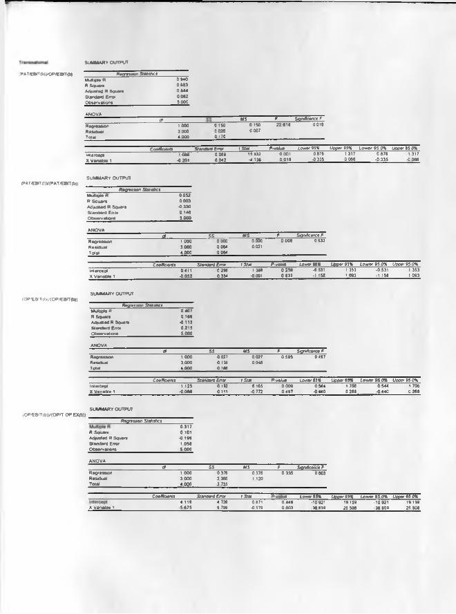
SUMMARY OUTPUT
<PAT/EBrrct>>yoP*BlT<b) ______________H u m a n S t t f lc iM u M ip M R 0 9 4 0
R S q u a r e 0 8 8 3
A d ju s t e d R S q u a r e 0 S 4 4
S ta n d a r d E r r o r 0 0 6 2
O b s e r v a t io n s ______________________________________ 5 0 0 0
A N Q V A
Of M S F S ig n ifica n ce F
R e g re s s * * ! 1 0 0 0 0 1 5 0 0 1 5 0 2 2 6 1 6 0 0 1 6
R e s id u a l 3 0 0 0 0 0 2 0 0 00 7
T o t a l 4 0 0 0 0 170
C o e tf io e n ts S ta n d a r d E rro r t S t a t P -v a lu e L o w e r 9 5 % U p p e r 9 5 % L o w e r 9 5 0 % Upper 95 0 %
in te rc e p t 1 0 9 6 0 0 6 9 1 5 83 2 0 0 0 1 0 8 76 1 31 7 0 8 7 6 1 3 1 7
X V a r ia b le 1 -0 2 0 1 0 0 4 2 -4 756 0 0 1 8 •0 335 •0 06 6 - 0 3 3 5 -0 0 6 6
( P A T i t B t T ( l ) V ( P A T / E B I T (b ) )S U M M A R Y O U T P U T
R e g re s s io n S ta tis tics
M u lt ip le R 0 0 5 2
R S q u a r e 0 0 0 3
A d ju s t e d R S q u a r e •0 3 3 0
S t a n d a r d E rro r 0 14 6
O b s e r v a t io n s 5 0 0 0
A N Q V A
j g __________________________ S S M S _________________ F __________ Sr&vficanceFR e g r e s s io n 1 0 0 0 0 00 0 0 00 0 0 0 0 8 0 9 33
R e s id u a l 3 0 0 0 0 06 4 0 021
T o t a l 4 0 0 0 0 0 6 4
Coeffcterti Standard Error f Slat P -v a t u e L o w e r 9 5 % U p p P r tS X L o w e r 9 5 0 % U p p e r 9 5 0 %
in te rc e p t 0 4 1 1 0 296 i 388 0 2 5 9 •0.531 1 353 - 0 531 1 3 5 3
X V a r ia b le i -0 0 3 2 0 354 -0 091 0 9 3 3 -1 158 1 09 3 -1 158 1 0 9 3
S U M M A R Y O U T P U T
( O P / E B 'T ( i ) ( / ( O P / E B l T ( b ) ) ____________________________
Represvon StatisticsM u fc p le R 0 4 0 7
R S q u a r e 0 1 6 6
A d ju s t e d R S q u a re -0 1 1 3
S ta n d a r d E m * 0 2 1 5
O b s e rv a t io n s 5 0 0 0
A N Q V A
Of S S M S F Significance F
R e g re s s io n 1 0 0 0 0 027 0 02 7 0 5 9 5 0 4 9 7
R e s id u a l 3 0 0 0 0 139 0 046
T o t a l 4 0 0 0 0 166
Coetfioents Standard Error t S t a t P v a tu e L o w e r 9 5 % U p p e r 9 5 % L o w e r 9 5 0 % U p p e r 9 5 0 %
In te rc e p t 1 1 2 5 0 182 6 165 0 0 0 9 0 54 4 1 706 0 5 4 4 1 70 6
X V a r ia b le 1 •0 0 8 6 0.111 -0 77 2 0 4 9 7 •0 4 4 0 0 26 8 -0 4 4 0 0 2 6 8
lOP'EBlT(b)V(OP'T OP EX(b))S U M M A R Y O U T P U T
Regression Statistics
R S q u a r e
A d ju s t e d R S q u a re
S ta n d a r d E rro r
O b s e r v a t io n s
0 3 1 7
0 101 - 0 1 0 9
1 0 5 6
5 0 0 0
A N Q V A
d f S S M S F S ig n ifica n ce FR e g re s s io n 1 0 0 0 0 376 0 376 0 3 3 5 0 6 0 3
R e s * J u a l 3 0 0 0 3 360 1 120
T o t a l 4 0 0 0 3 735
_______________________________________ Coeffiaenti_____________ S ta n d a r d E rro r_________ t Slat lue L o w e r 9 5 % U pp e r 95 % L o w e r 9 5 0 % U p p e r 9 5 0 %
0 4 4 8 .1 0 921 19 159 -1 0 92 1 19 159
36 8 5 9 2 5 5 0 8 - 3 6 8 5 9 2 5 5 0 8X V a r ia b le i
4 1 1 9
- 5 6 7 5
4 726
9 799
0 671
-0 57 9 0 6 0 3