A summary of TAU. A unified theory of physics.
117
A summary of TAU. A unified theory of physics. Andrew Holster. Draft from: Explaining Relativity. ATASA Research. August 2021. © Andrew Holster 2021.
Transcript of A summary of TAU. A unified theory of physics.

A summary of TAU.
A unified theory of physics.
Andrew Holster.
Draft from: Explaining Relativity.
ATASA Research. August 2021.
© Andrew Holster 2021.

1
Abstract.
This is a summary presentation of TAU, a theory proposed to explain relativity and unify physics. It is
a radical change, because it proposes six dimensions of space, instead of the usual three (normal
physics) or nine (string theory). It starts with an alternative foundation for Special Relativity, and
leads to a unified theory of physics. It is a realist theory because it is realist about space and time.
The TAU concept is briefly introduced here, and its results explained in three main areas, particles,
gravity and cosmology. In these areas it makes strong predictions and has several tests. This
presentation is based around these applications and the key questions of completing a full particle
model, and completing tests of gravity and tests of cosmology. These will decide its fate as an
empirical theory.

2
Contents
A Summary of TAU. ............................................................................................................................. 3
Introduction. ................................................................................................................................... 3
Preliminary. Explaining the STR metric. .......................................................................................... 8
The concept of TAU. ...................................................................................................................... 10
The torus geometry and electron model. ..................................................................................... 18
Space-proper time diagrams and Lorentz rotations. .................................................................... 19
The physical interpretation. .......................................................................................................... 22
Classical Electromagnetism. .......................................................................................................... 23
The particle geometry. .................................................................................................................. 27
Standard Model mass particles. .................................................................................................... 30
Particle generations. ..................................................................................................................... 33
Gravity. .......................................................................................................................................... 35
Global space. ................................................................................................................................. 41
Cosmology. .................................................................................................................................... 44
Transformations and evolution equations. ................................................................................... 47
Evolution of special quantities. ..................................................................................................... 50
Predicted rate of change of G. ...................................................................................................... 52
The time integration. .................................................................................................................... 59
The Cardioid solution for expansion. ............................................................................................ 60
Interpreting the cosmological predictions. ................................................................................... 63
Dark Matter. .................................................................................................................................. 66
Gravity and particle identity. ........................................................................................................ 70
Pilot-wave mechanics. .................................................................................................................. 74
Spin and non-local connections. ................................................................................................... 76
Bell’s theorem. .............................................................................................................................. 81
Entanglement and wave collapse. ................................................................................................ 85
Complex systems. ......................................................................................................................... 91
Metaphysics. ................................................................................................................................. 93
Answers. ........................................................................................................................................ 97
Appendix. TAU Project Summary. ................................................................................................. 99
References .................................................................................................................................. 101
Acknowledgements. .................................................................................................................... 116

3
A Summary of TAU.
Introduction.
This is a summary presentation of TAU, a theory proposed to explain relativity and unify physics. It is
a radical change, because it proposes six dimensions of space, instead of the usual three (normal
physics) or nine (string theory). It starts with an alternative foundation for Special Relativity, and
leads to a unified theory of physics. It is a realist theory because it is realist about space and time.
The TAU concept is briefly introduced here, and its results explained in three main areas, particles,
gravity and cosmology. In these areas it makes strong predictions and has several tests. This
presentation is based around these applications and the key questions of completing a full particle
model, and completing tests of gravity and tests of cosmology. These will decide its fate as an
empirical theory.
The aim here is to give an overview, in reasonable detail for generalists to see how the model works,
but with a minimum of theoretical derivations, so we do not get too bogged down in equations.
There are a lot of illustrations instead. Please note this is only a survey of the theory, and a more
detailed introduction with proofs follows in Chapters 2-6, where it is developed in stages. In the first
half here, we go quickly over the main concepts, in the second half, we give some equations for
cosmology and gravity solutions in more detail, because they are more novel.
Conventional Theories. TAU. Theories Are Unified.
Figure 1. LHS. Conventional theories do not quite fit together. RHS. We reorganise the
theories around TAU, which replaces STR in the center. This gives a single unified theory. Is it
true? That is the question. It has a number of fine-grained empirical differences with
ordinary GTR, QM and Cosmology. And a number of novel predictions and differences.
The state of the conventional theories is illustrated by the somewhat messy diagram on the left. The
theories just don’t quite fit together as a logical structure. It looks a bit like the digestive tract of an
artificial organism. This is evident in the problem of unification, the lack of a unified theory.
We make a list below of over thirty fundamental questions that physics cannot presently answer. A
unified theory should answer these, or help answer them.
TAU, the neatly organised structure illustrated on the right, is proposed as a theory that provides a
full unification, and it does provide answers to most of these questions. Whether they are the

4
correct answers is the other question of course. But it provides specific answers, and we explain
them as we go. A summary is given at the end.
Table 1. A list of questions physics cannot answer.
• What is dark matter?
• What is dark energy?
• Why are different measures of the Hubble constant incompatible?
• Did stars and galaxies form unexpectedly fast in the early universe?
• What is the quantum wave function?
• What is wave function collapse and what causes it to occur?
• What provides the space-like connection for quantum entanglement?
• Is there a deterministic level of physics underlying quantum mechanics?
• What is the speed and frame of reference for wave function collapse?
• Is it possible to transmit information faster than light?
• Is quantum mechanics the fundamental description of particles?
• Are the mass or charge parameters in the Standard Model related?
• Does the Standard Model represent the complete set of particles?
• Is there a reduction of the Standard Model to something simpler?
• Can particle masses or force coupling constants be predicted?
• Why do the electric charges of the electron and proton exactly match?
• What are the neutrino masses and can they be predicted?
• Why does the weak force fail time and space reversal symmetry?
• What is the quantum description of gravity?
• Why does gravity travel at the same speed as light?
• Is the black hole event-horizon singularity physically real?
• Is the black hole central singularity physically real?
• Is General Relativity fundamental or an approximation?
• What is the source of irreversibility of processes?
• Why are the laws asymmetric in time?
• Why are the laws asymmetric in space?
• What is the flow of time?
• What generated the low-entropy state of the universe?
• What will the future expansion of the universe be like?
• What happened in the very early universe before the Big Bang?
• Why is the universe made of matter instead of anti-matter?
• Do the coincidences in dimensionless ratios reflect physical relationships?
• Do the fundamental constants c, h, G change with time?
• How many dimensions does space have?
• Is String Theory the only way to generalise to a multi-dimensional space?
These are all important questions that current physics cannot answer. The range of questions shows
the extent of the problem. These are quite fundamental questions. They are not simply empirical
questions, to be answered by better experiments or by tweaking theories in the process of “normal
5
science”. They indicate fundamental issues with the theoretical framework. A unified theory should
answer at least some of these. TAU does: it provides answers to most of them. We explain these in
this chapter, and give a list of our answers at the end.
This list beings us back to the crisis in modern physics. Theoretical physics has been stuck with a
fundamental problem for over fifty years now – more than half its life-time. The two foundational
theories, quantum mechanics (QM) and the General Theory of Relativity (GTR), are incompatible
with each other, and no adequate consistent unified theory is known. QM describes forces and
particles on the small scale, in the Standard Model of particles. The Special Theory of Relativity (STR)
provides its mechanics in “flat space-time”. GTR describes gravity and space-time on the large scale,
and is the foundation for cosmology. GTR provides its mechanics in “curved space-time”. They are
successful in their own domains, but wherever they meet we find intractable problems. GTR cannot
be quantised, and the Standard Model of quantum particles cannot be merged with the curved
geometry. It is incomplete as a logical structure. Cosmology has introduced “dark matter” and “dark
energy”, which have gravitational effects, but cannot be identified with any particles in quantum
mechanics. Physics is now at an impasse on multiple questions.
This is unlikely to be solved without a successful unified theory. There have been many attempts to
create unified theories, including string theory, supersymmetry, quantum gravity, many worlds
quantum mechanics, Grand Unified Theories (GUTs), quantum determinism, discrete space-times,
and others. They all describe some interesting feature of physics. But none of the main-stream
theories has succeeded in providing a unified theory, and they look increasingly unlikely. They are all
about 50 years old, but have failed to work in the straightforward ways they were expected to. They
have come to look like theoretical mirages. And how many of the problems in our list above do they
solve?
Yet all the clues we have from different branches of physics seem enough to overdetermine the
solution to a unified theory, and we expect it should be obvious when it is recognised. It should
provide a clearly unified model, and have multiple points of verification. But it must go back to
something very fundamental. We will go back to the most fundamental level: the STR equation and
the number of dimensions of space. Our first step is to replace STR with a higher-dimensional metric
TAU. We have other material discussing this, so we briefly restate this. Then we consider how well it
matches the particle model and the gravity and cosmology models.
The questions in our list are general questions about physical reality, not specialised questions about
particular theories – except the last, which mentions string theory. This is the most pertinent place
to start, because TAU is distinguished by its multi-dimensional model for space. There are two main
types of modern theories: three dimensional space theories, and multi-dimensional space theories.
This is a fundamental divide. Either space is three dimensional, in which case multi-dimensional
theories will never work properly; or space has more than three dimensions, in which case
conventional theories will never work properly. We think the choice of dimensionality is a prime
feature to fix on.
String theory is fixated on nine dimensions, as the lowest possibility. But it has no specific model.
TAU proposes a six-dimensional spatial manifold. It has an extremely specific model. They are very
different, and disagree over almost everything. But they agree that the apparent three-
dimensionality of space may be illusory, and our identification of space as three dimensional,

6
through our senses is contingent. Additional spatial dimensions, to the three we recognise is entirely
possible in physics. In fact, it would be something of a coincidence if there were just three! It would
mean that we happen to see all the spatial dimensions, and space is represented to us completely,
by our innate 3D visual-spatial field. What about the possibility of other dimensions, curled up in
micro-dimensions? To think we see all the spatial dimensions through our senses may be illusory like
thinking that what we see in the visual spectrum of light are all the things that exist. But we cannot
see the air. Or the cosmic microwave background. Or colours in UV or infrared, that some animals
and insects and flowers use. We cannot see any fourth or higher dimension of space with our eyes.
But perhaps we can reason to them.
A more specific motivation for going to higher dimensions in physics is that 3D space just does not
seem to have enough complexity, in the spatial relations it provides, to explain all the weird and
wonderful phenomenon that physics has revealed over the last 100 years.
The underlying complexity of causation just does not seem
to fit into 3D space properly any more. In our view, it has
been abstracted into mathematical constructions –
complex wave functions, curved space-time geometries,
abstract algebras, non-spatial momenta, non-local
probability functions.
TAU proposes that most all this mathematical complexity
is generated out of a surprisingly simple six dimensional
geometry. The idea of a multi-dimensional geometric model for physics is no longer strange. But
what will be strange to physicists is the low dimensionality.
So far, string theory is the only extensively researched multi-dimensional theory, and it tells us we
have to start with nine dimensions of space (as a minimum). There is a “foundational proof” in string
theory that any higher-dimensional space (…for physics as we know it…) must have at least nine
spatial dimensions. This has prevented physicists from considering lower-dimensional spaces. But
TAU changes the assumptions of string theory, and finds a much simpler 6D spatial geometry that
works very well.
How is this possible if there is a general proof against spaces below 9D? Because TAU ignores certain
String Theory assumptions, and the string theoretic “proof” does not apply. We impose another set
of assumptions in its place, and it makes different predictions.
String theorists and other theory developers like to generalise from the algebraic forms and
symmetries of known equations – primarily covariance and gauge symmetry. These are in effect
assumed as the known forms for the laws of nature, as exemplified in ordinary QM or QFT or GTR.
String theory, supersymmetry, GUTs, and almost all other theories, are intent on duplicating these
formal-symmetry properties.
But TAU starts from a concrete model, which explains why STR works so well, and then why QM and
GTR work so well, but it does not imitate them, or copy their equations. It reconstructs them. We
must be able to re-derive known physics from a more fundamental basis in TAU.
“Quantum tunnelling! Entangled
electrons, Batman! Whats
happening to reality? Why the
instantaneous non-local wave
collapse for Plancks’ sake?”
“Careful with the language Boy-
Wonder.”

7
Figure 2. TAU predicts quantum particles, gravity and cosmology. It makes strong
predictions, and has a realist concept.
We will review TAU in these three areas in turn. They can be considered as three theories in their
own right. But they are bound by a fundamental model.
• A number of significant empirical coincidences are required for these three areas of the
theory to all work together.
• Several quantitative and qualitative coincidences required appear to be present at once.
• These are individually surprising, and even more striking as a whole.
There are several accurate predictions, relating diverse phenomenon in unexpected ways. This
represents the strongest evidence for the theory. Equally, strong predictions make it vulnerable to
empirical testing and failure. It can be tested at multiple points. Hence I had better finish writing it
up quickly before it is disproved.
A short statement of key claims for the present theory is given in Appendix 1. This summarises the
state of development in three parts: QM particles, gravity, and cosmology.
The aim here is to introduce and quickly survey the whole scope of the theory.
• The first step is the model for Special Relativity, particle physics and electrodynamics.
Because TAU matches with conventional physics closely here, we just observe how it
matches key points and equations of these conventional theories. We then discuss the
question of solving for the full Standard Model.
• The second step is the gravitational model, and we see how TAU gravity arises from the
physical model, and represents a kind of generalisation of GTR.
• The third step is the cosmology, and this is more novel, so we state the model in more detail,
and give some simple derivations. We review how it applies to measurements of gravity, the
Hubble constant and the age of the universe.
• Then we return to the unification of QM and gravity, where the two wave functions merge,
the model for particle-wave duality, the explanation of quantum entanglement and
interpretation of the wave function.

8
Preliminary. Explaining the STR metric.
We originally started in Explaining Relativity with the question:
• Why does the physical world behave relativistically, instead of classically?
• How can we explain the strange feature that relativity brings to the world?
The feature in question is most generally and simply seen as this. .
• Special Relativity tells us that when we move physical systems around in space, their internal
processes slow down. Everything runs at the rate: d/dt = √(1-v2/c2).
If you move things around, they slow down inside. Clocks slow down. Cells slow down. Molecules
slow down. Atoms slow down. Processes slow down. They all slow down, and in a way that exactly
compensates for their motion in space. It doesn’t matter what type of processes they are: electrical,
chemical, radioactive, mechanical, biological. The law is simple and the same for all: c2d2 = c2dt2 -
dr2. This is just the previous equation, squared and multiplied out by dt.
This is the defining equation of the Special Theory of Relativity. It makes everything in relativity
theory work. It pretty much is STR. Its primarily effect is to slow processes in moving systems. To
preserve conservation of momentum, this also requires mass to increase, with the familiar law of
mass dilation: m = m0. In turn this means the conserved quantity of energy is: E = mc2. These are all
the essential laws of STR. The Lorentz transformations follow from the metric too: for: c2d2 = c2dt’2
– dr’2 we must have: x’ = (x-vt) and: t’ = (t-vx/c2).
It looks completely innocent. But this tiny equation has led to a crisis!
The idea of explaining relativity will seem strange today, but it did not to Lorentz, Maxwell,
Fitzgerald and others who first encountered it. They sought a mechanical explanation for slowing of
clocks and shrinking of rulers, in terms of the aether. Unfortunately, a 3D aether does not exist.
Since Einstein and Minkowski, physicists have come to take the metric equation for granted, as the
unquestioned fact of the space-time manifold. The STR equation above is taken as the metric or
geometric function for “distance” in this manifold. As such, it is taken for granted: it is not explained
or explainable, any more than Pythagoras’ Theorem for distance in space, in classical geometry. It is
a fundamental fact of the representational space of modern physics. It is bound up in the tensor
calculus, the universal form of mathematical expression for laws of nature. To most physicists, it is
beyond the bounds of physical explanation, and it is just a fundamental law.
But we do question it, and ask for an explanation. It is responsible for all the strange behaviour of
STR. The fact remains it is weird. If you move things around in space, their internal processes slow
down, to compensate precisely for the motion. It entails physical effects, not just definitions of
geometry or coordinate systems. It is a great unsolved mystery of modern physics: how does motion
through space cause processes to slow down? Isn’t space invisible, and frictionless, with no
resistance to motion? Yet in STR, motion does have these effects! It slows processes down! It makes
things shorter! It makes things heavier! The relativistic effects of motion are all predicted from the
STR metric law above, along the principle of conservation of momentum. Also, the equation is not
just a geometric metric: it has the speed of light in it! A fundamental empirical physical constant! It is

9
about dynamics! And another thing: we know it is not consistent with curved space-time, in General
Relativity, or with cosmology. For a quick summary of the metric relation.
• The law: c2d2 = c2dt2 - dr2 is the defining equation of the Special Theory of Relativity,
• As a time differential it means: c2(d/dt)2+ (dr/dt)2 = c2.
• We can rewrite this as: √(u2+ v2) = c.
• We define: dw = cd and: u = dw/dt.
The second term is v2, the velocity squared, and the first term is the proper-time speed squared,
which we write as u2. So we can rearrange the STR equation as a Euclidean triangle law for a particle
with total speed c.
It means processes (u) slow down if their general speed (v) through space is increased.
Figure 3. Left. Space-proper-time velocity diagram. Middle. Space-proper-time
manifold diagram. Right. The triangle relation of STR.
We will visualise the relativistic relation through these space-proper-time diagrams, where we see
the STR law as a Euclidean speed metric, instead of the usual space-time metric. The metric can be
rearranged as a function giving the proper time speed from the spatial speed: d/dt = √(1-v2/c2) =
1/. Or inversely, as the real-time rate: dt/d = = 1/√(1-v2/c2). These equations are all equivalent.
Table 2. Arrangements of the Metric Equation.
Common arrangements of
the metric equation.
STR metric – divide by proper
time.
TAU metric – divide by real time.
Metric equation. c2d2 = c2dt2 – dr2 c2d2 + dr2 = c2dt2
ds2 = c2dt2 – dr2 ds2 = dw2 + dr2 = c2dt2
Differential equation. c2 = c2(dt/d)2 – (dr/d)2 (d/dt)2c2 = c2 – (dr/dt)2
Rearrange. Use chain rule:
(dr/d) = (dt/d)(dr/dt).
c2 = (dt/d)2(c2 – v2)
u2 = c2 – v2
(dw/dt)2+ (dr/dt)2 = (ds/dt)2 = c2
u2+v2 = c2
Rate of time flow. dt/d = 1/√(1 – v2/c2) = d/dt = √(1 – v2/c2) = 1/
Definition of Gamma. = 1/√(1 – v2/c2) 1/ = √(1 – v2/c2)

10
The concept of TAU.
TAU begins a simple concept, which changes a foundational assumption in the current interpretation
of relativity theory. The changed assumption is realism about space and time. It means that time and
space are different types of things. This leads us first to directly confront the fundamental law of STR,
the metric equation:
c2d2 = c2dt2 – dr2 STR metric – combining space and time.
Proper time Space-time manifold
The equation in this form reflects the normal interpretation, which combines time and space
together on the RHS, giving the space-time interval, and equates this to proper time, which is a
“physical invariant”, on the LHS. But given our assumption that time and space are different things,
we will reinterpret this, and separate space and time. The key role of time in our realist view is as the
differential operator for motion in a spatial manifold in which particles have trajectories. So we start
by putting time on one side, and proper time and space together on the other side, and instead of
modelling it as a space-time manifold, we interpret it as a “space-proper-time” manifold.
c2dt2 = c2d2 + dr2 STR metric rearranged.
Time Space-proper-time manifold
We want to combine proper time with space in a spatial manifold on the RHS. We first convert
proper time to its spatial measure, defined by the variable w:
w = c Definition of w.
We then define the metric on the space-proper-time manifold by:
ds = √(dw2+dx2+dy2+dz2) Metric for space-proper-time manifold.
This is a simple Euclidean metric for a 4D space. So we naturally write the relationship as:
𝑑𝑠
𝑑𝑡=
√(𝑑𝑤2
+𝑑𝑥2
+𝑑𝑦2
+𝑑𝑧2
)
𝑑𝑡 = 𝑐 The STR metric as a speed law.
Speed = 4D-distance / Time = Constant
This says: everything moves at the speed c in a 4D-Euclidean “space-proper-time” manifold.
This is still equivalent to the original STR equation, so far. Note the time-differential formulation is
perfectly valid, because the fundamental variables of STR are the 3D spatial trajectory function, r(t),
and the proper time function, (t), and both are fully parameterized by t for all particles or fields.
The general foundational assumption of classical and modern physics is that particles have analytic,
time-differentiable trajectories.
Note that the metric quantity of distance, ds, is defined in TAU so that: ds/dt =c, while in ordinary
relativity theory, the interval is defined on the space-time manifold as the interval: ds = cd . But the
latter is now just an ordinary spatial distance for us: dw = cd. We have rearranged the metric, and
we will reinterpret the model.

11
Speed in this proper time dimension will be: u = dw/dt, in analogy with: v = dr/dt, and we have:
u2+v2=c2 as two orthogonal components of speed in the space-proper-time manifold, or WXYZ
manifold. Similarly, momentum is: p = mu + mv = mc, as a vector addition. There is conservation of
momentum in each direction. We can put the equation in this form because the fundamental
assumption in STR, just as in classical physics, is that there are time differentials for the trajectory
and proper time functions for all particles and systems.
The STR treatment is focused on differentiating by proper time (to create 4-vectors). But remember
differentials in proper time do not exist for light, so a special treatment has to be given in STR. The
function gamma gives the rate of change of real time w.r.t. proper time. However for light, d = 0,
and has no value. Proper time cannot be used to parametrise the motion of light.
But the real time functions: r(t) and: (t) always have values. And differentials. If we differentiate by
real time, we get the TAU metric instead. And we have these simple relations in 4D:
u2+v2 = c2 Speed-vector addition in 4D.
p = mc = m(√(u2+v2)) Definition. 4D Momentum linear.
p = √((mu)2+(mv)2) = √(pw2+pr
2) 4D Momentum direction components.
E = p2/m = mu2+mv2 = mc2 4D Energy-momentum components.
Because of its complex space-time metric, STR normally starts with tensor calculus, which is a
formalism for dealing with differentiation in this awkward “metric”. But we have a nice simple 4D
Euclidean system, and we can analyze it by looking at simple examples that we can work out from
first principles. All we will need are basic principles of differential calculus. So we do not need to
start by writing down tensor equations. (And when we do, they are quasi-classical).
We can contrast two “metaphysical” views about space and time.
Table 3. Alternative Metaphysical Views.
Conventional STR
Relativist Assumptions about Space-Time.
TAU.
Realist Assumptions about Time and Space.
Time is fundamentally the same as space. Time is fundamentally different to space.
Time flow is unreal. Time flow is real.
There are no objective simultaneity relations. There are objective simultaneity relations.
Relativity theory requires a space-time
manifold.
Relativity theory requires a space manifold with
positions and time differentials.
Space-time is intrinsically curved (must use
Riemannian geometry).
Space is extrinsically curved in higher
dimensions (Whitney’s theorem).
Laws should be written in covariant form
(relativistic tensor equations).
Laws should be written as time differential
equations.
The Lorentz transformations are fundamental. The Lorentz transformations are contingent.
Space is not real separately from time. Space is real and it exists and changes in time.
Proper time is an invariant measure of
processes that occur in space-time.
Proper time reduces to a fundamental motion
in a (higher-dimensional) space?

12
The first line reflects a fundamental difference of opinion between realists and relativists. Although
relativism dominates modern physics, most people recognise that there are fundamental differences
between space and time. However, most physicists today would probably be confident of the
Relativist viewpoint, and reject the Realist views. But it is not until the last line that we reach the
starting point of the difference in physical theories that follow.
Now ordinary STR postulates space-time as a universal manifold for physics. It is a lot like God for
physicists. Processes obey the general law of STR above, as if they are all in a single space-time
manifold together. But there is no further explanation of this law in conventional physics. It is simply
a fundamental property, nominalized as the space-time interval, a property of an abstract space-
time manifold. It has no further explanation. It is just eternally how things are, in the modern view.
The TAU proposal is to replace space-time with a real WXYZ spatial manifold and give a reductionist
mechanical explanation for STR instead. But this can only work if we can reduce all the particles to
wave modes of one geometric manifold at once. When we develop the theory, we will start with an
example of adding a single circular dimension to a 1D space – giving a cylinder in 3D. We have w
curved in one dimension (meaning it is really rotating in two dimensions around the YZ-plane), with
free motion in an open third x direction. We can develop this geometrically into a space-proper-time
diagram, which we call a WX diagram, by unrolling the circular surface.
Figure 4. The “Compton-De Broglie Circular Light Clock”. This is a 1+2 = 3D space. If we set
the radius to give the energy required to represent an electron mass with a single wave, we
find it matches the fundamental relationships de Broglie and Compton found around 1923-
24 by equating: hf = mc2, and showing the equivalence of mass and light.
We can call this the Compton-de Broglie CLC because the relations we impose between the radius
and the mass-energy are what Compton and de Broglie discovered around 1923-24. We see these
shortly, but we continue with the concept of the geometric model for the moment.
• The STR metric equation applies precisely to describe the motion of particles or waves at the
speed c on a cylindrical surface like this.
So the geometry has an essential equivalence to the STR “metric relation”. But it describes a
different model, because we interpret proper time, , as the motion in w, which is now a motion in
an underlying dimension in a real space. This may seem a strange thing to do, of course, because
proper time is defined and measured quite differently to space. But the point is that there is a good

13
physical interpretation. And note that instead of postulating the STR metric as fundamental to
describe this model geometry, it is now a contingent property of the model.
• The geometry will ensure we get relativistic relationships, the Lorentz transformations, etc.
The typical quantum properties generated by this full-wave-length model are:
Full wave-length particle.
x = Wc/v = h/mv Spatial wave-length = de Broglie.
T = W/c = h/mc2 Period of wave-fronts at fixed (w,x) point.
f = 1/T = mc2/h Frequency of wave-fronts at fixed (w,x) point.
E =hf = mc2 Relativistic QM energy.
L = muR = ћ Intrinsic angular momentum = spin-1.
= ћq/2m0 = Lq/2m0 Magnetic moment.
The angular momentum is because: L = muR = (m0)(c/)(R) = (h/W)(W/2) = ћ.
A rotating particle with charge q would generate the classical loop current magnetic moment: = IS,
where I is the current and S is surface area.
I = q/t = q/T = qm0c2/h Current.
. S = R2 = ћ2/m02c2 Area.
Hence: = IS = (qm0c2/h)(ћ2/m02c2) = ћq/2m0
Considered from the ‘outside’ the system has a period, wavelength, rest-mass, relativistic mass,
intrinsic angular momentum, and (for a charge) intrinsic magnetic moment, all conforming to an
archetypal relativistic quantum system. We now use this to propose a reductive explanation of
fundamental quantum mechanical particles. It obeys special relativity, and it gives a novel way of
explaining why STR governed all processes except gravity.
We imagine that CLC systems existed on a tiny scale, and we could detect the proper-time periods
TA and TB, and the spatial wave-length, and angular momentum, but could not see into the
mechanical construction. We are aware of the motion of the system in X, but not the internal
motion in the additional dimensions YZ. In this case, the CLC particles will appear to us like
relativistic quantum particles.
This amounts to introducing an underlying realist geometric model for “proper time”, w. Note that w
is not taken as a “pseudo-spatial dimension”, like time in ordinary relativity theory, which is given an
“imaginary dimension”, ict, in the tensor formalism. The new dimension w combines with (x,y,z) to
give a space with a simple Euclidean distance metric. All the dimensions: (w,x,y,z) will be treated
identically in respect of their intrinsic properties as space.
Now for the general connection to quantum mechanics, we will find that solutions for waves in this
geometry obey this wave equation:

14
±(∇𝑤2 Ψ + ∇𝑥
2)Ψ =1
𝑐2
𝜕2
𝜕𝑡2 Ψ Wave equation for manifold.
This does not depend on any assumptions from quantum mechanics: it is simply obtained from the
geometry. And when we put in a mass to determine the radius, we will find that this matches the
relativistic QM Klein-Gordon equation – the most fundamental relativistic wave equation in QM
This solution occurs because of the circular boundary condition on the w space. This BC means we
can give velocity boosts to a wave or trajectory in the x direction, but not in the w direction. The
latter would involve spinning coordinates around the circle or pipe of w. But position is absolute in
w, and in all valid coordinate transformations for this geometry, we have: dw = dw’.
• A physical model for “proper time” as a spatial motion is only realistically possible if w is
cyclic, and on a tiny scale.
These are the boundary conditions on w. It must be cyclic to ensure that the new dimension has the
same properties of locality as XYZ space. It must be tiny so we do not normally notice it.
Now the example above works for light on a cylinder. But we are going to do something radical, and
propose that we can model all physical processes in a geometry of this kind. That is, we are going to
try to reduce proper time for all physical processes to motions in a similar type of geometry. We will
keep our normal XYZ space, and add some underlying microscopic cyclic dimensions for w, and call
this WXYZ space. This will be the space-proper-time manifold.
For this to work, w has to have more than just one dimension (otherwise all we could get is a kind of
simple boson, as in the example of light above). We will add two new w-dimensions, called we and
wp, and we will take these as the surface dimensions for a torus. These combine in a Euclidean
metric: dw2 = dwe2 + dwp
2. The torus rather than the cylinder above will provide our fundamental
geometry. This means there is a third dimension, through the torus volume. But that is all we will
add!
• Our fundamental model of space will consist simply of a torus embedded in XYZ space.
• Any point in the 6D volume can be represented by 6 Cartesian coordinates:
• (w1, w2, w3, r1, r2, r3).
• Points on the 5D torus surface can be represented by 5 surface coordinates:
• (we, wp, r1, r2, r3).
• Because the surface points have a boundary constraint in 6D:
• w3 = f(w1, w2, r1, r2, r3).
Now the idea is that motion in w in our theory will completely replace the normal variable , i.e.
proper time, in STR – for all fundamental processes! We start with the torus because it is a unique
manifold that can model the electron, which is the fundamental elementary mass particle, with the
lowest rest mass (apart from the ghostly neutrinos, which we will see is a construction).

15
Figure 5. LHS. The electron-proton torus. The electron is identical to a light wave that rotates
around a microscopic torus with a half-turn around the minor circumference. RHS. The torus
is embedded continuously in 3D space.
Note that particles or charges can pass each other much closer in ordinary XYZ-space than the torus
radius Re, which we will find is about 10-13 m. But they cannot pass much closer than the minor torus
radius, Rp, which is around 10-15 m. For the electron wave motion:
• The electron particle-wave does two rotations around the large circumference for a full
wavelength, turning 180 degrees on the small circumference with each full rotation.
This is the essence of the fermion model. To clarify the variables:
• The capitalised terms: We and Wp are taken as the circumferences, and Re and Rp are the
radii. (Note Re goes to the center of the torus pipe.)
• We take we and wp as distance variables on the surface, so that: dw = √(dwe2+dwp
2) is
distance on the surface.
• The full metric when we add motion in ordinary space is: ds=√(dwe2+dwp
2+dx2+dy2+dz2).
Now before we examine the solutions, we emphasize a general point about the explanation.
The motions in w are going to completely replace proper time, and the fundamental metric
equations will change like this.
STR View | TAU View
c2d2 = (c2dt2 - dx2- dy2- dz2) | 0 = c2dt2 – (dx2 + dy2 + dz2) – (dwe2 + dwp
2)
(QM) (TAU)
Plus the boundary condition on we,wp.
We move proper time from the LHS in the STR equation to the RHS of the TAU equation. It becomes
a description of a purely spatial process in the TAU equation – which no longer has a term for proper
time at all! In fact, it is just the STR equation for light in the higher-dimensional space.
This change of the fundamental equation reflects the fact that it will have to be a very powerful
reduction! Everything incorporated into proper time in physics will need to be reduced to a purely
spatial process – in six dimensions. We must do this via the atomistic reduction that the Standard
Model already represents. I.e. we only have to reduce the Standard Model particles and forces, and
all other processes in conventional physics (except gravity) will reduce through this.

16
At first this may seem almost impossible: the geometric model we introduce looks far too simple to
contain all the complexities and parameters of the quantum Standard Model! But surprisingly, when
we try, it actually appears to work! To reproduce all the processes of physics means that there must
be strong reductionist relationships inherent in nature, and this is what we have found.
Note that this way of extending space dimensions is quite different to the conventional concept,
which simply adds more space dimensions to the space-time metric. I.e. we can add additional
dimensions of space: w1, w2, … wn, to the STR metric like this:
c2d2 = (c2dt2 - dx2- dy2- dz2- dw12- dw2
2- … - dwn2) String theory extension of space.
This retains the form of the STR space-time metric, but with more space dimensions. It has the
normal pattern for a “covariant equation”. It now defines a space-time interval in 4+n space-time
dimensions. This is the lesson normally taken from relativity theory: since space-time is fundamental,
a generalisation of the STR equation must retain this form. But that is really just a guess based on
thinking that we recognise a fundamental mathematical pattern – or a metaphysical assumption
based on the belief in space-time as a kind of metaphysical reality.
TAU is fundamentally different, and it is not based on retaining the space-time manifold as the
fundamental assumption. This is why TAU is radically different to string theory, or any other
conventional theories based on taking the form of the space-time metric as the fundamental law.
So now we need to show how to derive key results from first principles of this geometric model. That
is really all there is to it! To jump ahead to how to do this, our solutions must match with
conventional equations of fundamental physics. They are normally written as covariant equations.
This means they are written in a form like the metric equation. We briefly look at a few of these.
Figure 6. The recurring role of Compton’s wavelength in some of the most fundamental
equations of modern physics. Compton Wavelength. WIKIPEDIA 2021.

17
To orient ourselves, what are these conventional equations going to look like in our new model, with
space, time and proper time rearranged? Just like the STR metric, these have three parts, with space
and time differentials and an invariant. E.g. the Klein-Gordon has space and time on the left and an
invariant quantity of momentum squared on the RHS. We can briefly illustrate what happens with
the Klein-Gordon equation, as the paradigmatic example. This is one of most fundamental equations
in QM: component waves of particles in relativistic quantum mechanics are always K-G waves. Just
as we rearranged the STR metric, we can first rearrange this to separate the spatial and temporal
terms:
1
𝑅𝑒2 Ψ + ∇𝑥
2 Ψ =1
𝑐2
𝜕2
𝜕𝑡2 Ψ
(Different combinations of signs may be allowed in complex valued solutions, and they correspond
to particles and anti-particles, so we do not worry about the sign of 1/Re2 here).
• The length Re = ћ/mec is the Compton wavelength.
This plays the critical role: it converts from mass to length. The LHS in our rearranged equation now
has both operators dimensionally equivalent to: (1/Length2). But we have to unify these into one
operator, which will be a 4-dimensional Laplacian for a four dimensional space. The basic complex
valued wave solutions look like this:
Ψ(𝑤, 𝑥, 𝑡) = 𝐴𝑒(𝑖
ℏ)(𝑝𝑤𝑤+ 𝑝𝑥𝑥 − 𝐸𝑤𝑡 − 𝐸𝑥𝑡) Prototype K-G solution.
with: pw = mec and Ew = mec2 for a particle with mass me. These are the solution for a kind of K-G
equation arranged like this:
±(∇𝑤2 Ψ + ∇𝑥
2)Ψ =1
𝑐2
𝜕2
𝜕𝑡2 Ψ K-G equation for manifold.
We will obtain these K-G solutions purely from the geometry – not from any quantum mechanics.
They hold whatever we take the function to represent. We can take the real parts of the solutions
alone and these must provide solutions for real-valued waves in our geometry (like EM waves).
We generally interpret as a complex-valued wave function in QM, but we do not have to define
any interpretation for it yet. We return to the physical interpretation later.
This works if w is a cyclic dimension of space, with a cyclic length of: W = h/mc, which is just the
Compton wavelength: R = W/2 = ћ/mc. This is a result of equating: E = hf = mc2. The term hf is the
energy for light, and mc2 is the relativistic energy for mass. By taking the wave to move at speed c,
with one full wavelength around the circumference, we immediately get: f = c/W, so: hc/W = mc2.
Hence: W = h/mc, or: R = ћ/mc. In this way we can treat the term w as a spatial variable, like x,y,z,
but it must repeat in a cycle: w + W0 ≡ w, where W0 is the appropriate cyclic wave-length. This is the
additional boundary condition that lets us derive a K-G equation, and makes the model Lorentz
invariant.
So this is the basic idea. Now the first main result is to show that we can realistically model the
electron, photon, and electromagnetic field.

18
The torus geometry and electron model.
In the torus model above, the large radius is determined by the fundamental principle:
E = mec2 = hfe Energy principle.
This identifies the rest-mass energy for the electron in two ways, through STR (E = mec2) and through
the energy of light (E = hfe). The reason for identifying them is that we are going to model an
electron as literally consisting of light trapped in the cyclic geometry of the torus.
But because in the torus model, the electron wavelength is twice the circumference, (giving the
lowest-energy wave), the frequency is: f = c/2We = c/2Re. Hence: mec2 = hc/2Re, and this gives:
Re = ћ/2mec Fundamental length.
This is half the reduced Compton wavelength for the electron. The factor ½ is because of the double-
wave. So this length Re has to be the radius of the torus in our model. We can then solve for wave
functions on the surface.
Remarkably, the properties of frequency, angular momenta, magnetic moment, etc, calculated from
this model correspond to the QM properties of the real electron – i.e. QM wave frequency, intrinsic
spin, intrinsic magnetic moment, etc. When we work it out in detail, the general solutions are Klein-
Gordon waves, and when the spin components are interpreted, they correspond to the Dirac wave
functions for an electron.
• The torus geometry works for spin-½ fermions like the electron.
• The simple circular geometry works for mass bosons, if we take one full wavelength in the
circumference: = W = 2R = h/mc.
This is a general result of using this geometry – we get constructions essentially identical to fermions
and bosons. The double-rotation is the essential feature to give the fermionic behaviour, with the
correct spin-½, and SU(2) symmetry. If we represent the electron as a wave, it is like a double wave
moving around on a mobius strip.
Figure 7. WeWp-diagram (no XYZ dimensions shown here). The torus is developed as a flat
surface. The electron forms a double wave around the torus.
This predicts the intrinsic angular momentum correctly as ћ/2, and the magnetic dipole moments
accurately, and other features. It is the double-wave (or half-wave) geometry that produces the
properties of the real electron. The phenomenal properties of mass, spin, magnetic moment, etc,
can be calculated quite simply. It is generalised by solving the electron wave function. The solution is
separated into three parts, corresponding to the motion in the three different dimensions of motion
(with r the direction of motion in XYZ space):

19
Ψ(𝑤𝑒 , 𝑤𝑝, 𝑟, 𝑡) = 𝐴 𝑒(𝑖
ℏ)(𝑝𝑟𝑟 − 𝐸𝑟𝑡)𝑒(
𝑖
ℏ)(𝑝𝑒𝑤𝑒− 𝐸𝑒𝑡)𝑒(
𝑖
ℏ)(𝑝𝑝𝑤𝑝− 𝐸𝑝𝑡) Electron wave.
The first two components represent the kinetic and rest-mass energy and momenta. But the second
component contains a spin of ћ/2, and the third component contains a small mass-energy with a
second tiny spin component. But the relationships are not completely represented in this equation
alone because the second and third terms are cyclic, they represent angular momentum, so they are
the additional boundary conditions. These are extra linear relationships that match the Dirac
equation, and give rise to the spinor properties of the electron. In the Dirac equation, which is the
foundational equation of QED, they are imposed by adding the matrix terms to the SG equation. This
correspondence is what makes the model feasible as a relativistic theory of the electron and EM
interaction.
Space-proper time diagrams and Lorentz rotations.
Physics is normally visualized in space-time diagrams, and all the modern physicist’s intuitions are
tuned around this representation – which also corresponds to using covariant equations. But we
have seen how we can transform an equation from the usual covariant expression to an expression
suited to our space-proper-time model. And the corresponding use of space-proper-time diagrams
(or WXYZ diagrams) becomes the natural alternative tool for visualization. This involves quite a
change from the conventional visualizations. It may be difficult to adjust our intuitions, for those of
us brought up on space-time and the relativistic tensor calculus. We review WXYZ diagrams in the
early Chapters, because they are essential to visualize the physical relationships. In this section, we
briefly illustrate some of these.
To start with, what do Lorentz transformations look like in space-proper-time? If we give the plane
wave we saw above a velocity boost in some direction in XYZ space, there is no effect on the torus
dimension, w, because it is orthogonal.
• We cannot give velocity boosts in w, because motion in w is a rotation, and rotation is
absolute.
The invariance of proper time is usually referred to the instrumental definition of its measurement
(i.e. counting processes) in ordinary STR. In our model, it is referred to the absolute nature of
rotation. But it is similar: rotations in w can be counted in an absolute sense.

20
Figure 8. The Lorentz transformation induces a rotation-and-shear transformation of the
WXYZ space that we can call the Lorentz rotation. A purely classical rotation, left, would
change w’ in the new coordinates, but this contradicts the boundary conditions. The
Lorentz rotation corresponds to tilting the axes while retaining the w coordinates.
For instance, on a Lorentz transformation, the trajectory of the moving electron tilts into a spiral,
with component motions tilting into XYZ. Note that the Lorentz transformations do not change their
definitions at all – they are defined to make the STR metric invariant, and they make our rearranged
version of the metric as the speed function invariant in precisely the same way.
When this is applied to electromagnetic fields we see they transform exactly like the classical EM
field, with 4-vectors for momentum, current, etc. Except now we define 4-vectors in the 4D space
manifold, not in the usual space-time manifold.
Figure 9. The Lorentz transformation of the EM in the WX. The red and blue lines show the
current vector, for a charge rotating in w. The resultant force of the field of a source charge q
on a ‘test charge’ at field point x is always orthogonal to the 4D current vector. All
conventional 4-vectors, for momentum, current, etc, correspond to similar diagrams.
The WX-diagrams are especially useful to visualize the momentum and energy relationships in our
model. We briefly illustrate these without much explanation here.

21
Figure 10. Left. A stationary and moving particle (blue) with the same rest mass in the WX
velocity diagram. They both move at the speed of light, c, in WX. Components of velocity are
red vectors. Right. The momentum components in the WX momentum diagram.
The components in w represent the rest-mass and rest-momenta (p0 = m0c), while the components
in x represent the ordinary momenta. This is our version of the momentum 4-vector, with the 4-
vectors now in 4D space (WXYZ) instead of space-time. Transfer of momenta must balance in each
direction. But we now see we have conservation of momentum in w just like x,y,z.
Note that a single particle cannot simply split into two particles with the two momentum
components – this contradicts the energy law. This is illustrated by the transformation of a
stationary particle to a moving state, through a ‘collision’ with another particle.
Figure 11. Two particles interact on the left, and there is a transfer energy and momentum,
resulting in two altered particles on the right. This illustrates the photo-electric effect.

22
A light particle with all its momentum in x strikes a stationary mass particle, and imparts some
momentum to it. But it cannot be simply absorbed into one particle - the solution requires a
reflected light particle. We need to assign a momentum and mass to light, written here as: p1 and p3.
• These momentum-energy diagrams apply to all interactions – including the EM, strong and
weak interactions, which are all orthogonal.
This illustrates that STR interactions are like classical interactions between particles with motions in
orthogonal directions. This is perfectly valid to describe conventional STR processes, but the
orthogonality of rest-mass momentum with linear momentum cannot be illustrated in conventional
space-time diagrams.
The physical interpretation.
Although we generally have the same relationships in TAU as in conventional STR, the difference
comes when we look at the physical interpretation.
• In TAU, all fields and particles must correspond to vibrational modes or distortions of the
underlying manifold.
The electric field corresponds to a rotating (tilting) vibration of the electron ring into XYZ space. This
behaviour corresponds to the usual 4-vector transformations of the EM field, where moving electric
charges have their electric fields tilted partially into magnetic fields. But it is caused by a rotating
mass-charge affecting the space.
Figure 12. This illustrates the electron torus tilting into ordinary space. The electric field is a
vibration of this kind, with the electron ring vibrating longitudinally w.r.t. ordinary space.
The rotating electron mass vibrates the torus, and creates the electric potential wave of a charge
(and later, a strain effect creates gravity.) This shows the fundamental problem of solving the model:
solving the vibrational modes of the 6D WXYZ space.
Vibrational modes in 6D may be rather difficult to analyse in general. But we know what the effects
must be in this case, from standard theory EM theory, so we can match the solutions to
conventional physics, and pick out the specific modes that correspond to the EM force. The model

23
needs to effectively reproduce the conventional electrodynamic model. Next is a short summary of
some of the relevant concepts of classical EM theory that we must link our model to.
Classical Electromagnetism.
For a phenomenological theory, matching with classical electrodynamics, we can assume the
electron has an elementary electric charge, -q, rotating with the wave, and this gives rise to the
classical EM field. (The electron charge matches literally to a classical photon trapped in the torus
geometry. We later take this rotation to be the source of the charge.) The proton has the opposite
charge, +q.
The EM force in the real world essentially comes back to the fields produced by just these two
“point-like” charged particles, e- and p+, electrons and protons, as they move around in space. Their
charges produce electric potential fields. There are also “free EM fields”, photons, containing energy
but no charge. The motion produces magnetic fields, but there are no magnetic charges.
In TAU there is really just one elementary electric charge, produced by the electron/positron wave.
This is wave is duplicated in the proton, spinning in reverse, giving an elementary positive charge. So
we really only need to produce this. In the Standard Model, protons are composed of three quarks
with fractional 0 in the Standard Model (+2/3, -1/3, +2/3), but there is no physical observation of
these charges, and no explanation of why they come in fractions of the same elementary charge of
the electron. In TAU, the electron and proton charges are produced by an identical mechanism.
Charges produce potential fields, and these produce EM fields, E and B, which are classically
described by Maxwell’s equations. The latter are often taken as the fundamental equations, but they
are not really. The force fields are not fundamental: they are constructed from the potential field.
• Charges produce a spherical scalar potential field, .
• Changes of , produced by accelerations of charges, produce vector potentials, A.
The potential field, (or V) at a point in space, represents the electrical energy per charge. The
spatial gradient gives the electric (force) field, E. This has a direction. The potential fields from
multiple charges superpose linearly. The potential field spreads out dynamically, as a spherical wave
travelling at speed c from the central point of a charge. (Note we will limit the charge radius to be
larger than Rp or Re.)
• In EM theory, the potential field is governed by a retarded wave equation. The wave travels
outwards from the point-like central particle.
• The solution in three dimensions is the spherical harmonic function: 1/r.
This is illustrated using light-cones in space-time diagrams. (Here we switch to V instead of - we
use V in TAU and in ordinary EM theory.)

24
Figure 13. LHS. Space-time diagram of charge stationary at r = 0. The potential V(r,t) at field
point r at t results from the potential field of the charge q at t’. The potential field travelled
at speed c spherically outwards from the charge. RHS. A second charge, qb, blue, is moving
towards the field point V(r,t) when it crosses the first charge. The retarded distance rB’ is the
same as for the stationary charge it crosses.
In the second diagram, the moving charge qb is closer to the field point r by the time t. But its electric
field at (r,t) turns out to be equal to that of a stationary charge remaining at rb(t). Although the
potentials contributed from both charges originate from the same retarded source point, the electric
field produced at the field point (r,t) by the moving charge is larger, because the gradient of the
potential at the field point is greater for the charge B, because of its motion.
Figure 14. Lines of equipotential V in a space diagram (x,y). These are all at one moment, t.
Left, stationary charge. Right, moving charge. The equipotential are circles (spheres in 3D)
spreading out from the central charge.
The potential wave spreads out spherically at the speed of light, whatever the particle motion. Note
that the equipotentials remain circles (spheres) on a Lorentz transform. But the equipotential circles
for the moving particle become bunched up ahead, giving larger E-field from: V at field-point (x,t).
V at (r,t) depends on the retarded position of the charge, when it produced the field that travels to
(r,t). This is the intersection of the backwards light cone from the field point to the charge.

25
This is represented by retarded potentials:
∅(𝑥, 𝑦, 𝑧, 𝑡) = 1
4𝜋𝜖0∫
𝜌(𝑥′,𝑦′,𝑧′,𝑡−𝑟/𝑐
𝑟𝑣′𝑑𝑣′ Scalar retarded potential.
A(𝑥, 𝑦, 𝑧, 𝑡) = 𝜖0
4𝜋∫
𝑱(𝑥′,𝑦′,𝑧′,𝑡−𝑟/𝑐
𝑟𝑣′𝑑𝑣′ Vector retarded potential.
(E.g. Lorrain, Corson, Lorrain, 1988, p.680-81). Note this has the retarded time variable, t-r/c. Note
that the intersection point of the world-line of the charge with the backwards light cone is invariant
w.r.t. frame of reference.
• The terms in t are asymmetric – the retarded equations are not time symmetric.
• This means electrodynamics with source charges is irreversible at a fundamental level.
Only the retarded solutions are physically real. There is a second set of mathematical solutions to
the wave equations, called the “advanced wave solutions”, but these are not physically possible.
They would describe the time reversal of normal physics. But time reversed physics does not work in
reality. Advanced wave solutions are not physically possible.1
This is the point where retarded fields enter into conventional electrodynamics, and similarly into
TAU. This retardation is equivalent to the causal principle, that physical effects (waves) spread
outwards from central causes (charges).
To illustrate how this leads to the Maxwell equations for E and B, we start with the classical non-
homogenous wave equation in the scalar potential function: = (r,t). This is the fundamental wave
equation, with the space-time operator on the LHS, and an invariant, the charge-density, on the RHS.
We will derive the Maxwell equation for E.
∇2𝜙 − 1
𝑐2
𝜕2𝜙
𝜕𝑡2 = −𝜌
𝜖0 Wave equation in (x,y,z,t).
∇. 𝑨 = −1
𝑐2
𝜕𝜙
𝜕𝑡 Definition of A.
Note that the first equation is the fundamental relation to the source charge, the second defines the
vector potential, A. We can see how this connects to the Maxwell field equations.
∂ 𝛁.𝑨
𝜕𝑡= −
1
𝑐2
𝜕2𝜙
𝜕𝑡2 Rearrange definition of A.
∇2𝜙 + 𝛁.𝑨
𝜕𝑡= −
𝜌
𝜖0 Substitute A in wave equation.
∇. (∇𝜙 + ∂𝑨
𝜕𝑡) = −
𝜌
𝜖0 Rearrange.
𝑬 = −∇𝜙 − ∂𝐴
𝜕𝑡 Definition of E.
∇. 𝑬 = 𝜌
𝜖0 Substitute to get Maxwell’s 1st equation.
1 So why is electrodynamics usually claimed to be time reversible? Because we can write a general wave equation that does not specify the time direction. However the actual law of physics is the retarded equation. It is irreversible. The fact that we can write a mathematical equation to describe the time reversal of processes does not mean those processes are physically possible.

26
The electric field is thus constructed from the scalar and vector potential fields – and the vector
potential is constructed from the scalar potential. This illustrates that the field (or its four partial
differentials, in 3D space and time) is what is fundamental. The field is produced by source charges,
which is the fundamental connection between charges connected to point particles and fields across
space produced by charges. The vector potential A is defined from the differentials of , and the
electric field E is determined from these.2
In TAU, we similarly take the charges, but now with an underlying motion in 4D (or actually, in 5D,
but we start with the 4D model). In our 4D space, we can rearrange the equations like this (we will
replace with V in the context of TAU):
∇𝑟2𝜙 +
𝜌
𝜖0=
1
𝑐2
𝜕2𝜙
𝜕𝑡2 Wave equation in 3D space-time.
∇𝑤2𝜙 =
𝜌
𝜖0 Postulate. The rest charge density.
∇𝑟2𝜙 + ∇𝑤
2𝜙 = 1
𝑐2
𝜕2𝜙
𝜕𝑡2 Rearranged.
𝑐2 ⊡2 𝜙 = 𝜕2𝜙
𝜕𝑡2 Laplacian in 4D.
Note that our 4D-Laplacian (box operator) here is not the d’Alembertian from special relativity. We
have rearranged the construction to represent our 4D spatial model (as with the K-G equation and
STR metric equation). The postulate now states that the rest charge is equivalent to the Laplacian
component in w. The source charge term now appears as a component of the total 4D field. In 4D,
5D, and in constrained spaces, there are different harmonic functions to the 3D harmonics. But since
there is no overall dispersion in our circular dimensions, they integrate to finite classical spherical
wave functions, once we are outside small atomic distances: > Re. This integration can be done,
and we can reproduce something almost the same as the classical laws – except now we have a
difference: multiple light-paths (potentials) connect the same events. We must integrate and
renormalise the electric potentials. We expect the same behaviour as in QED.
This illustrates how we can connect our model end-to-end with EM theory and QED at fundamental
points, and obtain the equations from an underlying physical mechanism. And the mass-wave in the
torus essentially duplicates the Dirac equation, and conforms to QM properties.
So now: what about all the other particles?
2 Of course there are non-trivial solutions without source charges, viz. free EM fields, or photons. But they are also defined by solutions for the potential field equation with zero charge density, i.e. for the homogeneous wave equation.

27
The particle geometry.
So far so good. This defines two nice particles, the electron and photon (which we get as the free EM
field as usual). But the idea is to use this single manifold to model all the particles! It is now it is a
matter of looking to see if other particles can fit. The next particle we construct is the proton.
There is a second dimension in the torus, the small radius, with wave solutions similar to the
electron solution. This must correspond to a second larger stable mass particle, and the only possible
candidate is the proton. So we postulate that the small torus dimension has the radius: Rp = ћ/2mpc
to match the proton mass. Now this length is about 1/1836 of the electron-ring radius, Re, so the
torus is very skinny. (Because: Rp/Re = (ћ/2mpc)/(ћ/2mec) = me/mp = 1/1836).
The proton has a short wave-length, hence a large mass-energy, and it will contain an electron-like
wave function as a component wave. It will require this lower energy level to be filled to be
energetically stable. The positive charge of the proton is produced by its electron-wave component,
but it must be rotating in the opposite direction to the electron, i.e. a positron.
“Because protons are not fundamental particles, they possess a measurable size; the root
mean square charge radius of a proton is about 0.84 - 0.87 fm (or 0.84x10⁻¹⁵ to 0.87x10⁻¹⁵
m.)3 In 2019, two different studies, using different techniques, have found the radius of the
proton to be 0.833 fm, with an uncertainty of ±0.010 fm.4” Proton. Wikipedia.
Hence the charge radius and physical radius are very similar to the ½ Compton radius.
Table 4. Energies and Compton wavelengths for four main long-lived particles.
Energy-Mass-W-R-T
Model photon
Neutrino TAU Model
Electron e-
Re = h/2me
Proton p+
RP =h/2mP
Neutron N
RN = h/2mN
e- masses E/mec2 1.48E-07 1.00 1,836.15 1,838.68
Energy (GeV) E = hf 7.58E-08 0.511 938.3 939.6
Mass (Kg) m = E/c2 1.35E-37 9.11E-31 1.67E-27 1.67E-27
W (meters) W = c/f 8.18E-06 1.21E-12 6.61E-16 6.60E-16
R (meters) R = W/2 1.30E-06 1.93E-13 1.05E-16 1.05E-16
T (seconds) T = W/c = 1/f 4.34E-15 6.44E-22 3.51E-25 3.50E-25
We see that the ½ Compton wavelength that we adopt for Rp is very close to (20% smaller than) the
measured average charge radius and physical radius. This match makes the model possible.
Essentially, the electromagnetic force and gravity operate outside the radius of about 10-16 m, while
the strong and weak forces only operate within this distance, which corresponds to the physical
boundaries of the torus. Note also the proton ring can be rotated into ordinary space at this scale –
forming a 3-sphere.
But we also need a third particle, the neutron, which is universal in nature, like the electron and
proton. It is similar to the proton, also a spin-½ fermion, but slightly heavier, and has no charge. But
there is simply nowhere for a wave representing this in the simple solid torus. It requires another
dimension, with the radius: RN = ћ/2mNc. It must be slightly smaller than the proton. And because of
3 Shearer, Paul. 2013. Antognini, Aldo, et al. 2013. 4 Bezginov, N. et al. 2019. Xiong, W. et al. 2019.

28
the similarities with the proton, it should be parallel with the proton motion. There is only one
apparent choice, which is to make the torus hollow inside. Thus we arrive at the basic TAU torus
model, which looks like this.
Figure 15. The micro-torus geometry. It has three parameters, the radii, which are fixed by
the masses of the electron, proton and neutron, me, mp, mN. It is embedded in XYZ space.
We use W’s for circumferences and R’s for radii.
The neutron is modelled as a wave on the inside of the pipe. It has a mass about 2.5 electrons more
than the proton. The neutron must contain two electron-wave components – an electron inside the
pipe, a positron outside – moving in opposite directions, so the electric charges cancel.
The neutron can therefore decay to a proton, as a lower energy state – because its mass energy is
slightly larger, and its momentum is in the same direction - but to do so, it must have some way of
transferring its momentum through the pipe, and the result must be to split into an electron and a
proton. When we work out the details, this corresponds nicely to properties of the neutron and to
neutron decay. But for this process there must be an electron neutrino, to balance momenta. And
we find the perfect candidate for the neutrino is in the electron model already!
The main electron spin is around the large circumference, We. But there is a secondary spin, around
the pipe, Wp. The wave (which may be initially imagined as carrying a point-like mass-charge around
the torus) completes one rotation of Wp for every two rotations of We, and so the momentum vector
in Wp is tiny. This means the electron has two dimensions of motion in w (not counting its XYZ
motion). Again, WX diagrams are useful to work out geometric relationships.
Figure 16. The 1-D electron as a wave motion in x, we and wp. The double-wave motion of
the electron gives strong relationships between the motions in the different dimensions.

29
These motions correspond to two wave components, and two orthogonal components of the
electron rest mass. The spin-wave in Wp has a very tiny mass-energy compared to the main electron
mass-energy in We. (This secondary spin momentum also weakly connects the electron with the
main proton mass wave.)
• This tiny spin-energy component is identified with the electron neutrino.
This is a novel prediction (and electrons do not contain neutrinos in the Standard Model). Perhaps it
is not absolutely certain that this has to be the interpretation of the neutrino. But it is very hard to
avoid. When we calculate the extra tiny spin-mass, it turns out to be 0.075 eV (or twice that, 0.15
eV). This is consistent with current empirical estimates, although they are not determined to better
than a scale of magnitude yet. Only the sum of the three neutrino masses is known with any degree
of accuracy, and is currently estimated between about 0.1 – 3 eV (opinions vary a little). Three
electron neutrinos on our model would be about 0.22 eV (or 0.45 eV). We cannot predict the masses
for the muon and tau neutrinos yet, but expect them to be comparable.5
So while this prediction cannot be empirically confirmed to better than an order of magnitude yet, it
is consistent, and this is quite a coincidence. The coincidence lies in the large difference of scale
between the neutrino mass, and the electron and proton masses that it is calculated from: they
differ in scale by about 10-6 – 10-9, but the result conforms to within a scale of about 10.
In summary, the TAU torus provides a remarkably good model to host the five major long-lived
particles to start with: the photon, electron, proton, neutron, and electron neutrino. (And their anti-
particles, which are reversed wavefunctions).
But is there room for the full set of particles in the Standard Model?
5 A guess based on dimensions is that the muon neutrino is about 12.25 times the electron neutrino mass.
30
Standard Model mass particles.
The model so far may seem far too simple. Yet we propose that it is all we need for all the Standard
Model particles and forces!6 Is this possible!? The Standard Model has about 24 particles, with their
own parameters, while so far we have only three or four independent parameters, and five or six
particle types. So how could such a simplistic reduction be possible?
Only by powerful coincidences between the geometry and the physics.
The geometry contains several further types of mass-waves. We cannot work these all out yet, but
we can match general features and scales.
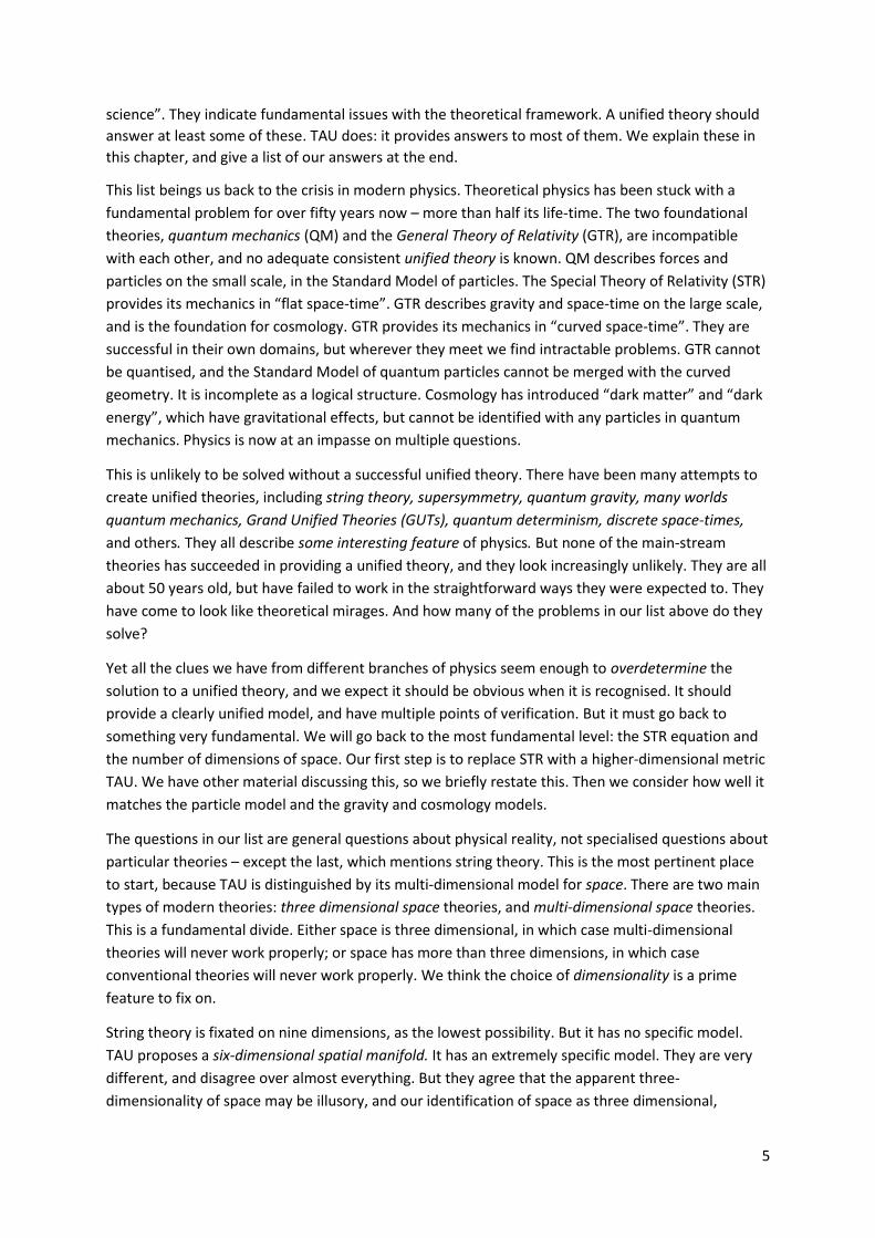
Figure 17. Three particle generations in the standard model. We can model the first
generation using the simple torus geometry, and then consider the 2nd and 3rd generations.
We have only so far only considered surface waves, travelling at c, in 5D (the WeWp surface plus 3D
XYZ space). The odd dimensionality is important, as it allows coherent waves. But there are also
waves possible within the volume, such as waves reflecting between the WN and Wp surfaces. These
volume waves will behave differently to surface waves. We do not know what speed they will travel
at without some additional principle. But they can only have very short wavelengths and high
energies and short life-times. They will not form stable particles, because there are many lower-
energy modes to decay to. So we expect very brief transitory particles. And there are also wave
combinations and masses plausible for mesons and other composite particles.
The torus pipe has a thickness, given by the difference: Rp – RN, between the neutron and proton
radii. This is the smallest physical length in the model so far, corresponding to a large mass. On the
assumption that waves in this dimension also travel at speed c, the energies and times are on the
scale of the transitory W+,W-, and Z bosons. These are close to the heaviest particles in the Standard
Model. (In fact waves in: Wp – WN correspond quite closely to the vector boson energies, while the
radius: Rp – RN is about six times too large. This is only an estimate until wave functions are properly
solved, but this is a good match to scale.)
Note also that there are two distinguished directions: in the plane of the torus, and parallel to the
axis of the torus. These give rise to two slightly different components in the proton and neutron
6 When I first developed the model, I assumed there must be more dimensions (probably 9), or more structure in the geometry. And there may still be. But everything now seems to point to just this simple structure.

31
waves. Up and down quarks will have to be identified with components in these two directions. But
up and down quarks are still pretty fuzzy in the Standard Model, their individual masses are barely
known to within 20% (only their difference is known precisely), and they can never be individually
observed. They also make up only one percent of the total proton mass in the standard model, the
remaining energy is attributed to a flux of gluons, which we will associate with internal energy that
strains the torus.
We see here the division of two realms of particles – which matches between the Standard Model
and TAU. Long-lasting stable particles like electrons and protons have to match directly to real stable
particles in TAU, and they do. But quarks can only match with wave components in TAU, and vector
bosons can only match with transitory particles.
But there is a fundamental difference between TAU and the Standard Model in this respect. The
scheme of TAU particles is more like the construction of complex atoms made by filling in electron
orbits from the bottom up with increasing energies, rather than a mathematical construction from
combining algebraic groups of elementary particle properties. To illustrate:
Figure 18. Illustration of TAU particle components. The neutrinos are electron neutrinos. The
electron* is a positron, and is a T*-reversed electron. As we go up, the rest masses (energy)
increase, and the w dimension changes.
The electron, proton and neutron thus all contain lower-energy wave components. Energy levels
must be filled from the bottom up for the particles to be stable. The neutron can decay to a proton,
creating an electron and anti-neutrino in addition. This means some particle constructions are
reorganised compared to the Standard Model. But there is a basic correspondence with mass, length
and time scales of the Standard Model particles.
Figure 19. The particle mass series, from electron to the top quark. Subsequent mass groups
are like 20-story sky-scrapers next to the previous group.

32
Table 5. Particle mass groups.
The mass range for a group generally spans about the mass of the lightest particle, from m
to about 2m. The gaps between groups are much larger than the variance within groups.
There are a four elementary but composite particles included: pion (lightest meson), proton,
neutron. Then the charmed b meson, as the heaviest meson. The W- and Z bosons are left out. They
are both about the same as the W+. All the other fundamental particles are shown, except photons
and gluons, which have no rest-mass.
Physicists would normally consider these in terms of their particle group types. But note that there is
a regular series of steps in the rest-mass groups. What causes this? A physical geometry that allows
multiple wave function components, and can make stable particles. As a whole, the Standard Model
mass particles reflect about 5 distinct mass scales, separated by about 5 orders of magnitude. This is
a strong pattern. And there is an excellent correspondence with these scales in TAU. This makes the
model possible.
The torus dimensionality also corresponds to the number of forces. The forces must transfer
momentum from W directions into XYZ. The EM force must connect We and XYZ (with the photon
being a vibration tilting the We ring into XYZ.) The weak force connects Wp and XYZ. The strong force
connects: WQ = We X Wp and XYZ. There can only be three independent quantum forces in TAU. The
relative strengths are also consistent.
So overall, the torus has the right structure to reproduce the first generation of the Standard Model,
and about the minimal complexity and dimensionality and mass-energy scales for the whole range.
But the main feature missing so far are the three generations of leptons and quarks.
Particles Mass MeVRatios between
groups Distance/Gaps
electron 0.511
up quark 2.3
down quark 4.8 185.9 Distance
strange quark 95 19.8 Gap
muon 105.7
pion+.0.- 139.6 9.9 Distance
proton 938.3 6.7 Gap
neutron 939.6
charm quark 1275
tau 1777 4.5 Distance
bottom quark 4180 2.4 Gap
charmed b meson 6276
bottom 9460 19.2 Distance
W+ boson 80380 8.5 Gap
higgs boson 125,100
top quark 173,210

33
Particle generations.
This triple structure of generations is the key pattern of the Standard Model. The structure for the
first generation (electron, proton, neutron) is duplicated at a higher energy level (electron → muon),
and then a third time (muon → tau). We can first look for the muon to solve the problem of
modelling generations in TAU. This single additional particle should give us the fundamental
mechanism for understanding generations, and should conclusively determine the interpretation.
On the other hand, mesons and quarks could also be modelled, and the W+,W- and Z-bosons can
also be modelled, so there are several lines of investigation, with strongly determined data and
limited modelling possibilities.
This means the full theory must be very solvable – all the clues must be there to solve it if it is
solvable. Other theories have investigated geometric properties in different ways, e.g. GUTs, seeking
to unify the forces, and although these have not quite worked as thought, they show strong patterns
of a similar kind to TAU.7 However, the question is how flexible TAU is to incorporate new features,
such as the multiple generations. Although the simple TAU model is very constrained by its fixed
geometry, it has more flexibility when we consider the dynamics of the geometry.
The muon is essentially an exact copy of the electron, but with about 207 times the mass. But there
is simply no place for the muon in the fixed electron-proton torus, without some new feature of the
geometry. The electron already occupies the lowest energy for the electric charge. We can try
higher-energy superposition states for higher-masses, but we get higher charges, and this does not
seem to work at all.
The key alternative is the dynamic distortion of the torus. There are local effects of energy on the
spatial geometry. The torus is not an inert entity – it already vibrates in EM fields, and strains in
gravitational fields. But another type of distortion is possible: a change of length ratios, from the
ratio: Re/Rp = 1836. This can plausibly change in high-energy collisions, because particle energies are
contained in the stretching of the torus space. The distinctive mode of change is as follows.
Figure 20. The TAU torus may change its length ratios while retaining its volume. The
minimum is a 1/150-ratio to Re, when all the radii are made equal.
7 There are some parallels with GUTs (Grand Unified Theories), which appeared tantalisingly close in the 1970’s, but did not quite work. They also identify particles and forces in terms of a small number of symmetry groups. However they are patterns in abstract geometries, and based on gauge symmetries, while we propose the symmetry groups will be found to correspond to our specific concrete geometry in 6D, and we will eventually see that we must adopt a definite gauge.

34
The torus is elastic, but obeys a law of conservation of 6D volume. To conserve the volume, we must
conserve the quantity: ReRp2, because the torus volume is: 22ReRp
2.
• Actually, strictly speaking our hollow torus is: 22ReRp2- 22ReRN
2 = 22Re(Rp2- RN
2), but we will
assume the ratio of the proton to neutron radius is fixed as a constant, call it a, so: Volume =
2 2ReRp2(1-a2), and we can work with ReRp
2 as the simple invariant.
Hence we introduce an average radius: RA = (ReRp2)1/3 as an invariant length characterising the torus.
I.e. no matter how the radii change relative to each other, locally we always have the same value for
RA. But note in the expanding universe, the real conservation law is:
• RURA = constant, with RU the universe radius.
We will get back to this, and it is the reason the particle theory has to be consistent with the
cosmology and gravitational theory, which both involve dynamically stretching space.
In terms of a ratio to the electron radius, this average radius is:
RA = (ReRp2)1/3 = Re(Rp/Re)2/3 = Re(1/1836)2/3 ≈ Re/150 Average radius.
This ratio: (Rp/Re)2/3 = 1/150 is a kind of magic number in the model, because it is the invariant
volume-average under (local) distortions of the torus.
• RA is the minimal radius of the torus, when the hole in the centre disappears, and the two
radii become equal: RA = Re’ = Rp’.
This distortion of the torus, expanding the proton radius to: Rp’ → 12.25Rp, and shrinking the
electron radius to: Re’→ Re/150, gives a wave-function solution like a very heavy electron, with 150
times the mass, and still one negative electric charge. The real muon is 207 times the electron mass,
so this is in the right mass scale. But the muon a bit heavy for the simple model. But we may
wonder: how much energy does this distortion really take?
This is also close to another “magic number” of electrodynamics: the fine structure constant, =
1/137. This suggests: (Rp/Re)2/3 ≈ = q2/40hc, which we also propose as a lawlike relation. Another
coincidence is that we must integrate the electric field energy down to exactly: Re to get the mass
energy: mc2 = hc/re to match the electrical self-assembly energy: hc/rE = hc/re or: rE = re = re/137.
Note the torus radii could only be made smaller than this minimum value (with the same volume) by
also changing the ratio of Rp to RN. This is possible too, so there are in fact several ways the torus
could distort to host muon or tau particles without altering the general topology.
There is another variable also: the speed of light changes when the surface tension changes, and this
modifies the simple mass-length relationships. These relationships merge in cosmology, where the
expanding universe also distorts the torus.
So to make further progress, we need to analyse all the dynamic quantities of the torus together.
But before proceeding further, we need to see how further properties are determined by
considering gravity and cosmology. So we will leave the Standard Model now, and move on to
gravity, which gives a new set of relationships. We return to particles subsequently, when we return
to apply the gravitational-cosmological model, and examine the features of wave function collapse,
non-local connections, entanglement and the interpretation of the wave functions.
To summarise, the particle model has very strong features for the first generation of particles and
the EM force, it makes strong predictions and none have broken down yet, and with the torus

35
stretch and other features, there is just about exactly the right complexity to get all the particles and
forces. At first it looks too simple, but if we make it any more complex we will probably get too many
particles and forces. There is ample data and several clear paths to continue the modelling.
However, the results of the TAU particle model will have to be consistent with standard particle
physics, as this has such strong data, and we should not expect novel predictions here.
Gravity.
The main areas where predictions of TAU do diverge from standard theory are in gravity and
cosmology. And this is where the most direct tests are found. The TAU theory for gravity is fairly
simple, and its main features have been worked out. There is not much choice in this. It departs
slightly from conventional GTR, and is empirically very testable. Gravity is produced by mass-energy
straining the manifold. The strain function uniformly expands the torus. This is how energy is stored
in the manifold.
Figure 21. Curvature in a simple pipe. The theory of gravity is determined by the strain
induced by a given mass-energy and the effect on the wave-speed, c.
Note the strain function does not really flatten out when we get close to a point mass. The main
solution is an exponential function, and produces a singularity, and this has to be modified at very
small distances. But in our solution, it does not simply flatten out. We return to this later. Here we
deal with the solution at significant distances from the mass centre.
Energy in this model is stored in the elastic strain of space, and the curvature this produces gives rise
to gravitational attractions. This strain represents potential energy – note that space itself is now a
source for storing energy. In conventional gravitational theory (or potential theory), we distinguish
between potential and kinetic energy. E.g. a test-particle m at a distance, falling towards a
gravitating mass M, gains kinetic energy, and to keep energy conservation, it is said to lose potential
energy.
Thus in a classical gravitational field, the potential energy is: EP = - mMG/r, and this trades off with
kinetic energy of: ½mv2. The potential energy is set at zero for a particle “at infinity”, and energy
conservation as it falls means: ½mv2- mMG/r = 0, and the velocity is solved by: v = √(2MG/r). The
field potential is written as: = -MG/r, representing the classical gravitational potential field.
Thus gravity (and other forces) involve a real exchange of potential and kinetic energy.

36
There is no equivalent representation of potential energy in conventional physics, where it is just
taken as a mathematical definition. It may be called the “field energy”, but the field has no physical
model. How is it “stored” physically? There is no mechanism.
In TAU, the potential energy for gravity is physically stored in the strain of space. The individual
particle mass-energies are also stored in their strains. When m falls into M, the combined strain as
they approach each other is reduced slightly, as the superposed wave-functions have a slightly non-
linear effect on strain. Thus the combined particle mass-energy when two mass particles approach
each other is reduced, and this is the reduction in gravitational potential energy. It must be
transferred to the kinetic energy. Thus we are able to have a fully realist model and realist
mechanism for energy.
Energy is stored in the strain of space, and the underlying strain of “empty space” represents the
background energy of space itself. Something keeps the giant inflated. We end up with an absolute
energy content for space. This is only possible because we have a realist model for space. It
corresponds to a cosmological constant in conventional GTR. It also means we do not have gauge
symmetry, except as a local approximation (instead we will have a strong scale symmetry). This is a
major point of departure from the conventional theories.
This also means that the energy “of space” can have local variations, e.g. clumping of internal
energy, on a galactic scale. This appears as “free energy” in space, which acts like a gravitational
attractor. This is proposed as the primary mechanism for “dark matter” in TAU. As galaxies evolve in
the expanding universe, they retain a larger background spatial energy (gravitational potential
energy) than the “cold” intergalactic space they are set in (due to the dynamic of transferral of
energy between space and matter in the expansion process). Such local distortions of the manifold
are like a kind of inhomogeneous fluid, flowing between regions, and self-attracting, and attracting
particle masses. This model for dark matter has no associated discrete quantum particle, it is free
energy of space.
Figure 22. LHS. This shows the development of the torus surface, as we approach a mass on
the right. Trajectories from left to right are moving towards the mass center. Straight-line-
motion on the cone development (blue) is a geodesic (almost). Rotation at constant x (red
line) is an accelerating path. RHS. The trajectories around w. For the straight-line path, the
increment x in the x-direction is not constant with each rotation. It accelerates into x. The
resulting geodesic is not actually a straight line, because the speed of light also changes.
This is a visualisation of the physical mechanism for gravity. Such a mechanism is only possible
because we have a realist model of space as an aether, with real properties of strain and energy. To
specify the theory of gravity, we just need to specify the strain function, and its effect on curvature

37
and the local speed of light in the surface. This turns out to be surprisingly simple, and gives a theory
matching GTR very closely – but with smooth solutions.
The strain produces two effects: an acceleration towards the centre from both the spatial distortion
(because the curved surface now acts like a funnel for particles or waves), and a change in the speed
of light. We now summarise the key equations of the theory. Particles are localised in XYZ, and the
strain function is a spherical function around the mass centre. This is a simple exponential function:
𝑅(𝑀, 𝑟) = 𝑅0𝑒𝑀𝐺
𝑐2𝑟 Torus strain function.
Here R is any dimension of the torus (such as Re), R0 is the value of R in empty space (or at infinity),
and r is the radial distance from a central source mass M. We define the function as K(M,r):
𝐾(𝑀, 𝑟) = 𝑒𝑀𝐺
𝑐2𝑟 Definition of K.
This strain function is determined by more fundamental considerations, reflecting the manifold
properties. It has the linear superposition property. If we take M to be composed of two masses: M =
M1+M2, the function gives the linear superposition: 𝑅(𝑀, 𝑟) = ( 𝑅0𝑒𝑀1𝐺
𝑐2𝑟 ) (𝑒𝑀2𝐺
𝑐2𝑟 ), and is identical to
imposing the two masses in sequence. Note that this equation is valid when r is substantially larger
than the torus radius, but when r becomes comparable to the torus radius it is no longer valid.
The result of the strain is this metric-speed equation at the field point:
𝑑𝑠
𝑑𝑡=
√(𝑑𝑤2
+𝑑𝑦2
+𝑑𝑧2
+𝑑𝑟2
/𝐾2)
𝑑𝑡 = 𝐾𝑐 TAU metric.
Here r is the radial vector to the field point, and y, z are orthogonal directions at the field point.
Again, this is derived from more fundamental properties of the continuum. This means that:
• The speed of light in the orthogonal directions w,x,y reduces from c to Kc.
• The speed of light in the radial direction r reduces from c to K2c.
Figure 23. The field point r is a distance r away from mass M. The ellipse around r shows the
surface speed, c(r), generated by the central mass M at the field point. The speed of light is
now different in the directions parallel and orthogonal to the radial vector.
The speed-metric is required by continuum properties. It corresponds to surface tension and to
speed anisotropy of light in an inhomogeneous medium. More generally, the solutions are
represented by 4X4 matrices representing speed tensors: cij. These correspond to the usual metric
tensor, g. The central mass solution is symmetric so it can have a diagonal form. We now compare
this with the usual Schwarzschild solution for GTR.

38
If we rearrange our speed metric, above, into the usual type of GTR line metric formulation, using:
d = cdw, it is:
d2 = dt2/K2 – dr2K2/c2 – dy2/c2 – dz2/c2 TAU Line Metric
We call this K-gravity. This is exactly the form of the GTR Schwarzschild line metric, except we have
used K (“big K”) whereas GTR uses this “little k” function:
k = 1/√(1-2MG/c2r) Definition of little-k
d2 = dt2/k2 – dr2k2/c2 – dy2/c2 – dz2/c2 GTR Line Metric
(This is normally written in spherical coordinates, we have defined: dy = rd and: dz = r sind as
local orthogonal coordinates at the field point.) The difference between the TAU metric and the GTR
metric is determined by the differences between K and k. If we expand K as a Taylor series, we see
that k is really the first two terms of K. It is easiest to see as:
1/k2 = 1-2MG/c2r Definition of k.
1/K2 = 1 - 2MG/c2r + (2MG/c2r)2(1/2!) - (2MG/c2r)3(1/3!)+ …. Taylor expansion.
They differ in the second-order terms: (MG/c2r)2 and higher. 1/K2 is the analytic continuation of 1/k2.
For the direct comparison of k and K:
k = 1 + MG/c2r + (3/2)(MG/c2r)2 + …
K = 1 + MG/c2r + (1/2)(MG/c2r)2 +…
Now the factor: MG/c2r is small in weak gravitational fields. Hence: k ≈ K + (MG/c2r)2 for large r, and
k is slightly larger than K. Hence the Schwarzschild solution will predict slightly stronger accelerations
than our K-gravity, for the same source mass. But note that for experiments in the solar system, we
estimate the value of GM for the sun from measured accelerations and the assumed theory, and
using K-gravity we must recalculate GM as slightly larger, and there is a kind of reversal of the effect
at larger radial distances. In terms of empirical tests:
• Current measurements of solar system gravity are not precise enough to distinguish
between the two predictions.
• But the differences can be tested with a practicable experiment in the solar system.
The difference will probably not be noticed accidentally by astronomers without a dedicated
experiment, because it requires an experiment designed around the specific effect. An experiment
to test this is explained in (Holster, 2017).
In fact, the TAU prediction initially appeared to be confirmed by the anomaly in the Pioneer
spacecraft data, which was in free-fall over 20-30 years.8 But it subsequently turned out that the
Pioneer data is too dirty to detect such fine anomalies. The Pioneer trajectory data initially showed
anomalies on exactly the scale predicted by TAU. And this was a problem for NASA for about 15
years. But through a decade-long effort to reestablish consistency with conventional GTR, the NASA
theorists searched for and found some extra small uncontrolled factors that were overlooked in the
8 Musser 1998; Bertolami et al 2003; Mbelek et al 2003; Nieto, Martin, Turyshev et al, 2003; Palle, 2004; Ranada, 2004; Turyshev, et al, 2012.

39
original analysis and design.9 However it is not particularly convincing. Given there were several
factors overlooked, and the theorists were looking for a factor to reconcile the data to a preferred
model (GTR), and the key factor found (a tiny heat asymmetry in the spacecraft) is based on a
complex theoretical analysis (not confirmed empirically), the Pioneer experiment cannot be taken as
a reliable test of such fine-scale effects.
It was just an accident that the Pioneer data turned out to be just sensitive enough to pick up this
scale of difference between TAU and GTR. Conventional tests of “alternative gravity” are limited to
testing a narrow range of variations of GTR, but these do not test K-gravity. (We discuss this in more
detail in the context of the Lunar Laser Ranging experiments, which are similarly claimed as strong
confirmation of GTR, but where the experiments also fail to distinguish GTR from TAU.)
To calculate the effects of gravity in TAU, we need a principle governing the motion of particles in
the “curved space”. This can be derived from first principles of the continuum mechanics, but
because principles of energy and momentum conservation hold, this turns out to be equivalent to
the usual geodesic principle in GTR, at least to an extremely good approximation. Applying this we
then find that:
• The K-gravity solution corresponds precisely to the GTR solution for a mass-density that is
slightly smeared out in space (to infinity), not a mass concentrated entirely in a central
region in empty space, as assumed in the normal Schwarzschild solution.
Smearing a mass out beyond a given radial shell reduces gravitational effects within that shell.
The substitution of K for k defines the K-gravity solution for g. But we can now reverse the usual
GTR derivation (from: T → g), and instead derive the stress-energy tensor T required to
produce this g (i.e. g → T). This is analytically solvable. We consequently obtain the pressure-
density distribution required to produce K-gravity in conventional GTR. The calculation shows the
mass-density (r) required to produce g for K-gravity varies primarily with 1/r4 for large r. The
series expansion in terms of 1/r is found to be:
= (M2G/4r4K2)+ (c4/8Gr2K2)((2MG/c2r)3/3! + (2MG/c2r)4/4! + …)
This solution shows something interesting about GTR. The defining equation is:
G = R + ½gR = (8G/c4)T Einstein’s Equation.
This equates the space-time metric G on the LHS to a function of the stress tensor T on the RHS.
Now G represents a geometric description in Riemannian geometry, and this purely geometric
description still holds for K-gravity. But the application of the equation requires the physical
interpretation of T, the empirical term on the RHS. This is calculated from mass-energy
distributions, requiring another theory. TAU forces us to reinterpret this term – as we must expect
because it changes the physical interpretation of mass.
TAU means that mass is never concentrated at a point, it is always continuously distributed to
infinity! The reason is illustrated in the strain diagram above. The presence of a mass continuously
strains space, the strain function is continuous and positive to infinity, and this is responsible for
9 Turyshev, et al, 2012.

40
gravity. Hence it is impossible to have T or with “sharp boundaries” or a discontinuity in space –
and so it can never go to zero.
Imposing: T = 0 outside a region, and: T ≠ 0 inside a region, as assumed in the derivation of the
Schwarzschild solution, means that T cannot be an analytic function across all space, and contains
a singularity or analytic discontinuity. (Indeed this discontinuity in the conventional mass distribution
is what really produces the usual black hole event horizon singularity.)
• K-gravity removes this singularity, and thus removes the black hole event horizon, normally
assumed to be a surface at: r = 2MG/c2 where quantities become infinite.
• But the curvature in K-gravity starts to become large around this distance, and it is still
effectively the “black hole radius”.
Hence the nature of “black holes” changes dramatically in TAU. Strictly speaking there are no black
holes as understood in GTR. But the curvature of space becomes large around the Schwarzschild
radius so that particles and radiation effectively can become trapped. Dense concentrations of
matter are still appropriately called “black holes”, and they occur when there is sufficient mass
density that the Schwarzschild radius extends beyond the normal physical radius of a very dense
object. But K-gravity predicts that “black holes” will behave quite differently in some respects to
those predicted by GTR. E.g. they can leak radiation, and proper time does not slow to zero and
quantities no longer become infinite.
The TAU alternative the GTR black holes remains consistent with observation. Although “black
holes” at the centres of galaxies are assumed to be GTR black holes in physics, a GTR event horizon
has never been observed, and its specific properties have never been confirmed. TAU would remove
one of the main conceptual anomalies of modern physics, and it makes “black holes” simpler.
This close match with GTR means TAU predicts a viable theory of gravity on a local scale, and it is
consistent with GTR at significant distance from the mass, but also has distinctive differences.
However we see another fundamental effect: straining space changes the speed of light, c. This is
evident in conventional GTR, as we already saw above. But in conventional GTR there is no
physical explanation or mechanism – it is just a result of the formal equations. In TAU, there is a
physical explanation.
The fundamental constant c characterises a property of space. It is continuum property, related
to the surface tension. When space is distorted, as under the gravitational strain, this changes.
We will soon see that all the “fundamental constants”, c, h, G, 0, as well as the elementary masses
and charge: me, mp, mN, q, must be taken to characterize properties of space in TAU. And they are
dynamic and can change with changing properties of space. Their values are not set in stone, for
all time, as magical values determined at the “creation” of “space-time” in a mystical “big bang”
event.
But this gravity theory now raises two distinct problems:
• What happens at the central singularity, when we approach r→0? Can we extend the K-
gravity solution to the centres of individual particles?
• Is K-gravity consistent for infinite space?

41
We will continue on with the second question, and we now return to our larger model of space.
Global space.
Our model means that at every point of ordinary 3D XYZ-space there are three more hidden
dimensions. So the whole space is a six dimensional space, with a five dimensional hyper-surface on
which ordinary long-lived particles are stable wave modes. But what is the topology of the large
space? The main problem with the basic K-gravity solution above is that in infinite “flat” space, the
volume integral of the strain function goes to infinity. I.e. a finite mass will produce an infinite
volume increase, in terms of the 6D volume. This is not physically feasible.
Instead we have to make space finite, and using the model we know from cosmology, i.e. the
expanding universe, we make XYZ space into a 3-sphere. It is extrinsically curved in a fourth
dimension, which is one of the torus dimensions. So we return to consider the combination of the
torus with ordinary space.
Figure 24. LHS. The torus embedded at points in a locally flat XY plane. RHS. On the
cosmological scale, XYZ is a 3-sphere, and the XYZ directions rotate into the w1 direction as
we move in a fixed direction on the surface. W1 is the axial direction of the torus.
Note first that the diagram on the LHS shows the torus at two points very close together in x. This
illustrates that two particle trajectories can interact at much closer distances in x than the large
radius Re. But the Rp is the natural limit. The electric charge spirals around the proton radius, Rp, and
cannot be localized more precisely in XYZ space.
Now Lorentz symmetry holds locally around a point, and space is “locally flat”. If the XYZ space
extended flat in all directions, as indicated by the LHS diagram, it would correspond to a globally flat
STR metric over infinite space. But this is not possible in TAU, because it would make the volume
integral of the strain function infinite (and it is incompatible with an expanding universe). Instead,
we make space a 3-sphere, a finite closed universe, and the volume integral becomes finite.

42
Figure 25. A particle imposed on an empty TAU universe strains the torus and increases the
6D volume of space. For a closed hyper-spherical universe, we can integrate around the
whole universe, and the extra 6D volume is finite.
The finite radius changes the strain equation and gravity equations we saw earlier to a slightly
modified form:
𝐾(𝑀, 𝑟) = 𝑒𝑀𝐺
𝑐2 (1
𝑟+
1
𝜋𝑅𝑈) Strain function in finite universe.
The additional factor of 1/RU comes from integrating the strain around the finite hypervolume. It is
extremely tiny and can be ignored in all local gravity. But it is essential for the global consistency,
and in the very early universe. And we see the strange feature that the radius of the universe enters
into the local equation for gravity!
(Note also that G and c are constants for “background space”, without mass present. Once we get
into the full theory we have to start distinguishing dynamic values for the constants).
Our first concern here is with the curvature, and construction of the hyper-space. The expanding
universe is described in standard cosmology by the Friedman equation, and curvature is treated as
intrinsic curvature, in the formalism of Riemannian geometry. We can generally translate our
solutions back into these conventional terms. But our underlying model is very different. We define
space as an extrinsically curved hyper-surface. This is not possible in conventional physics, with only
three spatial dimensions. Note also that we disentangle time from space by splitting the effects into
the spatial curvature, combined with the modification of the speed of light.
The striking point of difference is that space in TAU is an extrinsically curved 5D surface, bounding a
6D volume. Conventional physics treats 4D space-time as an intrinsically curved Riemannian
manifold. The formal possibility of switching to extrinsic curvature is ensured by Whitney’s theorem
(1933). But we do not just make a formal reinterpretation. We physically disentangle space from
time. Space and time are thought to be quite inseparable in GTR; but they are separable in our
slightly modified theory.
Space as a whole is then a kind of 6D aether. We should stress that our ordinary 3D space alone is
not an “aether” as C19th physicists thought of it: it is a “surface” of larger manifold. The 6D space as
a whole is a concrete manifold, with a finite surface, which can be distorted, vibrate, change shape.
It has real properties, such as a surface wave speed (the speed of light, c), an elasticity (related to G),
a 6D volume and a 5D surface area. A fundamental principle is that the total 6D volume of the
manifold is conserved under distortions. Such a property cannot even be conceived in conventional

43
theories. But it is natural and inevitable in TAU, and it is the source of very powerful theoretical and
empirical relationships and predictions.
Treating curvature as extrinsic may seem impossible to relativity theorists, but it is perfectly valid. It
is guaranteed that we can do this by a foundational theorem of differential geometry: Whitney’s
theorem (1933), which states that an intrinsically curved space in N dimensions can always be
modelled as an extrinsically curved hyper-surface in at most 2N dimensions – and if N is odd, at most
2N-1 dimensions. Any intrinsically curved 3D Riemannian space can be modelled as extrinsically
curved in 5D. The global curvature in our model is simple, and it can be modelled in 4D, with
ordinary space as the 3D hyper-surface of a 3-sphere.
This means that if we travel in a “straight line” in space, say in the x direction, the x-vector really
rotates. It does not rotate in the y or z directions, but in one of our w directions. By the time we are a
quarter of the way around the universe, the x-vector will point completely into the original w
direction. By half-way around, it will point in the opposite of the original x direction. It is precisely
analogous to travelling around on the surface of a sphere.
This also means that the fourth direction of curvature must be in a specific w direction. To make this
consistent and to match with the spin asymmetry of the electron, it proposed that this is the
direction of the torus axis. We will call this direction w1. It is always orthogonal to the we direction at
any point on the surface of the torus. It is parallel to wp from points on the outer or inner
circumference. (The direction of wp of course rotates as we go around the small proton
circumference on the torus). The direction of w1 rotates into x as we travel in any x direction around
the universe.
W1 also provides an asymmetric direction for the spin direction of the electron and proton waves in
the torus, and the asymmetric spin of the EM field. We use a “left-hand rule” to associate spin
direction of the electron with motion, just like spin direction of the magnetic field produced by
motion of electrons in a current. This is a major time asymmetry in particle physics. If the physics
was time reversed, we would have “right handed electrons”. This should not be confused with the
merely “conventional” labels for electric charges or magnetic fields. The physical asymmetry is that
only one direction of spin is allowed. The asymmetry is apparent in ordinary quantum mechanics. It is
often claimed that quantum mechanics the ordinary Schrodinger equation is time reversible, but this
is not correct, as only half the possible wave function solutions are allowed. (See Holster 2003(a) ).
Physicists get around this by defining time reversal for quantum wave functions as the combination
of true time reversal, T (which reverses both trajectory motions and spin direction), plus complex
conjugation, *, to restore the spin direction, and this is called the Wigner time reversal operator, T*.
This is adopted because T* is a real physical symmetry. But it is misleading about the symmetries.
The physical solutions are time asymmetric. This corresponds to the asymmetry of spin rotation in
our model.
We can now take spins to be “± into the w1 direction”. This spatial asymmetry – towards and away
from the cosmological center – also allows a physical basis for the asymmetry of the weak force. In
conventional theory, there is no underlying physical basis for a distinction of spatial directions.
• This model means that on a global scale, there is a unique frame of reference for space.

44
Locally, space is flat (STR metric), and we can transform between moving frames of reference, using
the Lorentz transformations. This holds for ordinary physics on a local scale. But there can be only
one consistent global frame in our model. This is essentially because rotation or angular momentum
is absolute. This is obvious in our model because we have extrinsic curvature, introduced through
additional dimensions of space.
This is seen if we consider sending light signals around a symmetric static universe. An experimenter
could send two light signals in orthogonal directions, x and y. They will eventually circle the universe,
and come back, and cross at the point they originated from. If the experimenter is in the true
stationary global frame, the light beams will cross where they started, back at the original position
of the experimenter. If a second experimenter is moving w.r.t. first experimenter, and sends two
similar light beams (when the two experimenters coincide in space), those light beams will follow
exactly the same paths, and meet back at the same point. But the moving experimenter will now
have moved to a different position, and will not be at the point where the light beams meet. The
experimenters will be able to tell whether they are really stationary w.r.t. the global frame.
We cannot expect that local covariance rules out a unique global frame of reference for the universe
as a whole. It is empirically evident in the unique “stationary frame” for the cosmic micro-wave
background radiation (CMBR). This is the frame in which the CMBR is isotropic. This special frame is
adopted in cosmology as stationary. The Big Bang cosmology makes no sense in other frames. E.g.
the “cosmological principle”, which claims homogeneity and isotropy on the large scale, can only
possibly hold in (at most) one frame. A moving frame induces relatively different concentrations of
matter and light in the direction of motion. This requires a global frame of simultaneity, and an
absolute frame of space. It contradicts the usual space-time metaphysics. But remember, we are
changing the number of spatial dimensions. That is the major change in the way we see space.
This brings us to the TAU cosmology.
Cosmology.
The global topology in TAU matches general features of standard cosmology, i.e. Robertson-Walker
models for an expanding universe, but only up to a point. It departs for the very early universe,
where conventional cosmology is a purely theoretical extrapolation. It similarly departs for long-
term future predictions. And it departs in the interpretation of dark matter, dark energy, the Hubble
tension, and gravitational constant, that are not explained by conventional cosmology.
At present the universe is expanding. The simplest solution from TAU predicts that the radius follows
a simple cyclic function, it will reach a maximum radius after a certain time, and contract again.
When it reaches a minimum radius, it will “bounce”, and go into new expansion phase. This solution
may be modified, but it is good to illustrate the mechanics. However the big difference in the theory
is that TAU requires that fundamental constants are dynamic, as they characterize properties of
space, and as space expands and contracts, constants change and processes will run faster or slower
as a consequence.
Now our conventional measured variables (for space, time, mass, charge) are fixed instrumentally to
physical (atomic) processes that are governed by the constants: c, h, 0, q, me, mp, mN, and we do not
normally notice this change – because all the local electromagnetic and quantum processes change

45
in unison. But gravity behaves separately, and we can measure changes in its relative strength to the
EM force, and predict discrepancies in measurements taken across large time periods. However
more generally, the fact that instrumental variables may appear unchanging to us does not mean
that these variables are adequate to write the laws of physics.
When we write the laws of physics in TAU, we have to adopt “true variables” for the laws to be
invariant over time. This time translation invariance is the most fundamental assumption of physics
– it is the assumption that there are unchanging laws of nature. We can have changing constants
without breaking this assumption, but they must be changing in a larger framework of simple
invariant laws. However the laws of TAU are not time translation invariant in our conventional
variables.
This gives the two key problems of the TAU cosmology.
• Constants c, h, G, etc, change values with expansion, and can be solved as functions of the
universe radius, Ru.
• Ru changes with time, and can be written as a function of time: Ru(t). This is the expansion
function, and it describes the history of the universe.
The first problem we can solve exactly – or at least, we propose an exact solution, which is
consistent with our larger theory. Whether it is the only plausible solution is really still an open
question. But this is a question that is simply not considered in conventional physics, and showing
how a solution works is important as a concrete example. For the second, I put forward the simplest
realistic solution I can think of, which has a strong logical consistency in the model. This is bound to
be modified, but again having a concrete solution is important to illustrate fundamental features of
the model.
This solution assumes a homogenous 3-sphere for space, characterized by one variable, RU(t). (I.e.
we ignore cosmological inhomogeneities – and the possibility of a spatially distorted universe. The
universe might also have an alternative topology, e.g. a 3-torus rather than a 3-sphere. We ignore
this here, and only consider the simplest possible solutions.
The problem is to model the expansion of the universe consistently with the effect on the local
micro-physics that happens in the torus.
Figure 26. Left, the universe at earlier time, t0. Right. At a later time t1, the hyper-sphere has
expanded, the torus has contracted. A particle (blue) strains space, and as the universe
expands the strain decreases. The solution must ensure conservation of total volume.
The fundamental principle is conservation of the 6D spatial volume. The aether acts like an
incompressible fluid, with a surface tension. The volume is essentially the product of the torus

46
volume X 3-sphere volume. The fundamental effect is that as the 3-sphere expands, the torus shrinks
to maintain the volume.
Figure 27. The expanding universe has two opposite effects. Local objects bound together by
EM forces, e.g. atoms, molecules, rulers, etc, shrink – as the torus dimension shrinks. The
universe as a whole expands – and unbound objects like galaxies separate.
As the universe expands and the torus shrinks, the real dimensions of atoms shrink, the real speed of
light increases, the real particle masses decrease, the fine structure constant is constant, the real
linear momentum is constant. Because of the scale symmetry, as the torus shrinks, all the objects
shrink with it. Rulers, clocks, us, etc. We are turning into shrinking people! Yikes! But we don’t seem
to notice. Locally, all the material objects locked together in strong energy relations are shrinking
together. But the opposite effect is happening on the astronomical-intergalactic scale: the distance
between galaxies (or objects not bound by local forces) increases, as they are separated by the
global expansion of space. This is the Hubble expansion. But to interpret it now, don’t we have to
take into account that light was travelling slower in the past? ... and what about gravity? If the
distance to the moon increases because of weaker gravity but the speed of light increases … or the
rate of supernova production was different in the part … or the luminosity of stars in the distance
ladder … our inferences about measurements are have to be recalculated.
The upshot is that we need to find transformations from conventional instrumental variables, which
are actually changing, into true model variables, which are not changing. These will be dashed
variables. Note that this only applies to the base units for: r’, t’, m’, q’, or their differential quantities:
dr’, dt’, dm’, dq’. This coordinate system is not changing. The instrumentally-defined quantities or
coordinates use the mass of atoms and periods of atomic processes to define space and time
measurements, and they are changing. This means fixing: me, mp, c, h, qe as constant. This defines
everything as constant by definition, except G.
It is quite well confirmed this works empirically: and the TAU model matches this result. Only G
appears to change, in instrumental coordinates. But what really changes? The TAU model starts with
the 6D volume conservation.

47
Transformations and evolution equations.
The exact 6D volume is: Vol = (/2)RU3RW
3, but ignoring the small constant of integration (/2) the
essential invariant is the invariant length, L:
L6 = RU3RW
3 = Constant Volume conservation.
But note that this equation only holds generally in the true variables, as we see. By the end of this
section we will switch to using dashed variables for the true variables, when we need to use them.
So we can continue to use our normal variables as they are.
We identify: RW = RA = (ReRp2)1/3 from particle physics: the average torus volume-radius that we
obtained in the particle theory. For a simple model we assume this is an average over a fairly
homogenous universe.
Note we use RW in the cosmology theory as a generic variable, and identify it with RA, as the specific
amount determined by the two masses in the particle theory. It is essential the radii are in this
combination, which corresponds to the combination of masses: mA = (memp2)1/3.
This is the topology the torus model for particles determines: the torus volume is the combination:
ReRp2. The invariance of this is the source of key relationships between local constants, that RA
depends on, and the global universe radius, RU.
Now: RA = ћ/mAc = ћ/c(memp2)1/3. (Again, we ignore the small factors of ½ for fermions here.) The
true quantities for: me, mp, c and ћ may all be expected to vary with expansion in our theory. To
solve the cosmology we must take into account changing constants, with changing basis units (our
instruments are shrinking), and use the special role of the present moment as the reference point in
the measurement of constants. It requires a set of transformed variables to represent, because it
means that the values of constants measured at the present moment change, and this means that
the basis units for space, time, mass and charge must change magnitude, in our normal system.
• So we define a transformed coordinate system with dashed variables, and their
relationships with the universe radius, R’.
A critical concept for this was recognised by Dirac (1969), who developed a cosmology in which the
constants may change: G, h, c, m, q. He started with a simpler theory (in 1937), but the first version
failed.10 It does not take into account that a transformation of variables is required. In the 1960s,
Dirac realised that a transformation makes more general solutions possible. If fundamental
constants change, basis units for quantities may also change, and we must transform from our
conventional system of “measured quantities” to a system of “true quantities” in which the laws are
written.
Dirac showed in principle how this can be done as a differential transformation. His own theory was
motivated by what he called the Large Number Hypothesis (LNH). Certain dimensionless numbers
can be constructed from fundamental constants and global variables: c, h, G, me, mp, q2/0, the age T,
radius R, and the number N of mass particles. The values of the dimensionless numbers have several
distinct coincidences. Although his theories were rejected, Dirac remained convinced that these
10 Dicke, 1961; Dyson, 1977.

48
“large number coincidences” reflect physical relationships for the rest of his life. The problem was he
had no model to determine how the constants should change, except to determine the Large
Number relationships. He just made an educated guess to get a theory going. It was slightly wrong
but a good idea. TAU gives a second version, but based on a more determined model.
Dirac’s theory relates the age of the universe (time) to the value of changing constants. However
TAU relates everything to the universe radius. We do not relate constants directly to time.
We first provide the variable transformations and evolution of the constants in terms of R. And then
solve the universe radius as a function of time, as seen in our own measuring system. We give
functions for the values of constants like c, h, G, etc, in terms of a normalised radius of the universe,
R-hat:
Ȓ(t) = RU(t)/R0 Normalised radius.
Here: R0 ≡ RU(t0) ≡ RU(Now) is the present radius, and t0 = Now is the present time for us. We must
recognise in the formalism that our measurements and observations are made at our present time,
when the universe radius and the constants have their particular values Now. We use the special
time variable: T with the origin: T = 0 set at the time of minimal expansion in the past (the Big Bang).
So T effectively represents the time since the Big Bang, which is what physicists generally call the age
of the universe. It has the same metric: dT = dt.
We can imagine physicists at a different cosmological time to us, say a billion years ago, who
measure quantities the same way as us instrumentally. Some of the constants will be changed, and
their basis units for time, space, mass and charge will be in a different system of physical units to
ours. E.g.
• If we both define mass using the mass of the electron or proton as a standard unit, the basis
unit for mass is reducing.
• If we both define length using the Compton radius of the electron: r = ћ/mec as a standard
unit, the basis unit for length is reducing.
This means there is a difference between true variables, and measured variables.
• The laws of physics must be written in the true variables to have their correct form to match
the model, which makes them time translation invariant.
Only in the true variables will the laws be simple and invariant and correspond to the model.11
So we assume that there is a system of true variables for space, time, mass, charge in which the laws
have their simplest form, and are time translation invariant.
• We will take: (x,t,m,q) as our conventional measured variables, and (x’,t’,m’,q’) as the true
variables, and establish transformations: (x,t,m,q) (x’,t’,m’,q’).
• Similarly we take: (c,h,G,me,mp,q,0) as our measured constants, and (c’,h’,G’,me’,mp’,q’,0’)
as the true constants, and establish transformations between them.
11 If we insist that comparison with some standard mass like the electron mass is the definition of mass, that would make the electron mass constant throughout time by definition..

49
The same issue arises for our radius variable: Ru and “age of the universe” variable: T. We must use
the true variables, Ru’, and T’, to define the fundamental laws, and subsequently transform them
back into our conventional variables, R and T to interpret ordinary measurements. We use
normalised variables for these as the key parameters in evolution functions.
Normalised variables.
Ȓ’ = R’/R0’ and: Ȓ = R/R0 Definition of normalised radius universe.
Ť’ = T’/T0’ and: Ť = T/T0 Definition of normalised age.
The true normalised radius variable: Ȓ’(T’) = RU’(T’)/R0’ is used as the parameter in our functions.
Note below we often write: R or R’ for the universe radius, RU or RU’, where it is unambiguous. We
generally use a subscripted 0 to represent present values. The basis unit transformations are defined
as differential transformations like: dt = f’dt’, where f’s are all simple functions of the normalised
radius, Ȓ’ = R’/R0’. The solutions for variables and constants in TAU are proposed as follows. We
simply state these here, and explain their rationale in more detail in a Chapter.
The variable transformations.
dx = Ȓ’dx' Space metric transformation
dt = Ȓ’2dt' Time metric transformation
dm = Ȓ’dm' Mass metric transformation
dq = Ȓ’dq' Electric charge metric transformation
The evolution equations for the constants in true variables.
c’ = c0Ȓ’ Evolution of speed of light constant.
h’ = h0/Ȓ’ Evolution of Planck constant.
G’ = G0 True gravitational constant is constant.
me’ = me0/Ȓ’ Evolution of electron mass.
mp’ = mp0/Ȓ’ Evolution of proton mass.
qe’ = qe0/Ȓ’ Evolution of elementary electron charge.
’ = 0/Ȓ’2 Evolution of electric force constant.
’ = 0 Evolution of magnetic force constant.
(These must be determined and justified from the underlying mechanics of the manifold.)
The transformations are completed by specifying boundary conditions at the origin:
Boundary conditions.
R → 0 as R’ → 0 Zero radius of the universe.
T → 0 as T’ → 0 Zero age of the universe.
And boundary conditions matching true and conventional values at the present time:
dx0' = dx0 dt0' = dt0 dm0' = dm0 dq0' = dq0
c0’ = c0 h0’ = h0 G0’ = G0
me0’ = me0 mp0’ = mp0 qe0’ = qe0 0’ = 0 0’ = 0
This defines the general system of dynamic constants proposed in TAU, and we can now solve the
evolution of conventional variables in terms of true variables.

50
Inverse evolution equations.
c = c’/Ȓ’ = c0 c is constant.
h = h’Ȓ’ = h0 h is constant.
G = G’/Ȓ’2 = G0/Ȓ’2 G is decreasing.
me = me’Ȓ’= me0 me is constant.
mp = mp’Ȓ’= mp0 mp is constant.
qe = qe’Ȓ’= qe0 qe is constant.
= ’Ȓ’2= 0 0 is constant.
= ’ = 0 0 is constant.
Note that all the conventional variables except G are constant. This is expected as they are defined
instrumentally. Conversely, all the constants except G vary with Ȓ’ in the true variables.
Evolution of special quantities.
Note that our conservation of 6D volume law holds in true variables, by substitution from above:
RU’RA’ = RU’ћ’/c’(me’mp’2)1/3 = RUћ/Ȓ’c(memp2)1/3 = R0RA0 = constant
But the 6D volume in conventional variables is not constant:
RURA = (R0RA0)Ȓ Volume in conventional variables varies with R.
This is an example of the fact that the laws of nature only appear correctly in true variables.
In true variables, constants change, to reflect properties of space, e.g. the speed of light reflects
surface tension, and it changes with expansion. But in conventional variables, the speed of all our
processes increases, including our clocks, so our measurement of time increases speed with light,
and our measuring instruments shrink, but the speed of light appears to remain the same. A quantity
may be constant in one system and variable in the other.
However dimensionless quantities have the same values in either system. There are only about four
independent dimensionless quantities.
• The fine structure constant, , is predicted to be constant:
= q2/40hc = q02/40h0c0 = constant = 1/137 Fine structure is constant.
This holds in either set of variables (because it is dimensionless), and it follows by substituting from
the equations above.
• The dimensionless ratio of electron to proton mass is also constant:
me/mp= me0/mp0 = constant = 1/1836 Mass ratio is constant.
And this means the average mass ratio is constant:
me/mA = me0/mA0 = (1/1836)2/3 = 1/150 Average mass ratio is constant.

51
This is why it is possible to identify: ≈ me/mA in our model. There is also a dimensionless constant
defined from c, h, G, m, which we call the Dirac constant.
• The dimensionless Dirac constant, D, changes with Ȓ’2.
D = ћc/mA2G Definition Dirac constant.
Substituting values from above:
D = ћc/(memp2)2/3G = D0Ȓ’2
We must use the mass combination: (memp2)2/3 in the theory, because this is the invariant average
mass corresponding to volume. Because D is dimensionless it has the same value in any variables:
D’= D Identity.
And there is one more: the dimensionless cosmological ratio:
• The universe – torus ratio changes with Ȓ’2.
RU/RA = (RU0/RA0)Ȓ’2 Universe/Torus ratio.
We then state the fundamental relation, that was predicted in a different form by Dirac, by equating
these two dimensionless constants:
RU’/RA’ = D’ = D Dirac-TAU relation.
But we can just take it as an empirical postulate for now. Substituting for the definitions, with: RA =
h/c(memp2)1/3 (ignoring the factor of ½) this predicts the radius of the universe from purely local
constants in its simplest form as:
RU’= RA’D = ћ’2/(me’mp’2)G’
This relation holds at all times, and we can substitute the present values: ћ02/(me0mp0
2)G0, and we
get the value as (the simplest possible combination, without geometric factors, except in ћ2:
RU0’ = ћ2/(memp2)G = 6.91 billion light years.
• Coincidentally, this is exactly half the measured age: 13.82 billion light years, times the speed
of light.
It seems a strong coincidence that this coincides with precisely half the measured age of the universe
times the speed of light. There are two main current methods used to estimate the age (time since
the Big Bang), which give measured values of about 13.77 - 13.81 billion years.
Now the age predicted by these methods is really giving us estimates, one way or another, of the
time it has taken light to travel across the universe from events, starting soon after the Big Bang.
So we have to predict the co-moving coordinates in TAU of this light, and this is what the result
seems to represent: the age times the speed of light. We are measuring how far the light has come,
and this seems to be what the TAU radius means, at first. The measurement of age from the CMBR
also measures how far the light has come from its production in the primordial universe, divided by c
to get the time.

52
Note that this result is the first Large Number Coincidence, that inspired Dirac to formulate his
theory. But he did not know exactly what to use for mass in the constant D, and he defines: D* =
ћc/mempG (giving the electron and proton equal weight). Also he took the ratio as between the
universe age and the characteristic electron time: TU/Te = D*, which corresponds to:
TU=ћ2/(me2mp)Gc. This is empirically wrong by about a factor of 100. He still thought this was a strong
coincidence – because we are combining multiple constants with large powers, on the scale of 10-30,
to produce a result within 103. But our torus model forces us theoretically to adopt a different
combination of masses: (memp2), and this gives an even more freakish coincidence!
Now our prediction almost looks like it is pointing to an exact relationship with the age of the
universe – in which case, where does the factor of ½ come from? Well, factors of ½ and 2 are
floating around in our geometry, and in the choice of h or ћ. E.g. we should strictly define Rw as half
the value taken above to conform to our electron-proton model. But we may also expect the
relation to predict a comoving-distance around the circumference, the comoving distance from the
light source, not the radius or total circumference of the universe. (The latter will turn out to be
more like 30 - 100 bly.) But we should not worry about the factor of ½ initially, or conclude that it
points to an exact relation yet. The close match to the exact measured age of the universe within a
factor of 2 can be considered the very coincidental result. But to interpret it, there are two more
questions.
First, our prediction is for the “radius” of the universe, in the true distance variable, RU0’. But:
• How does this prediction of a value for RU0’ relate to the conventional variable, RU0?
Second, the “coincidence” is that the predicted radius is related to the measured age, T0, by the
speed of light: RU0’ = ½T0c.
• But how does this predicted radius relate to the conventionally measured age in our theory?
(And what is the relation between T0 in conventional variables and the true age, T0’?)
We will next determine the transformations: R’ → R, which is also necessary to determine the
predicted rate of change of G in conventional variables. Then we return to the second question.
Predicted rate of change of G.
Note that our evolution equations above predict that:
• All the constants appear invariant in conventional variables except G (which actually just
conforms to the instrumentalist definitions of conventional variables), but:
• All the constants actually change in true variables except G.
Hence the primary measurable prediction is that:
• G in conventional variables is decreasing with 1/Ȓ’2 (in true variables).
This predicts the rate of change of G w.r.t. the true variable, Ȓ’. But what we measure in experiments
to determine the rate of expansion (the Hubble constant) is the rate of change w.r.t. the
conventional variable, Ȓ. And this is determined from measurements made at the present time – but

53
referring back (through light sources from various types of stars) to distant events in the past. We
have to translate the prediction for G into Ȓ.
We can relate R and R’, using the differential transformations above. We integrate using: dR/dR’ =
dx/dx’ = Ȓ’, and use the boundary condition that: R → 0 when R’ → 0. (We will not assume a
singularity in R’ or R at the temporal origin, just a very small minimal value of R’ and R close to the
time origin we set for T.) For an arbitrary radius, R1, we take the definite integral:
R1 = ∫0,R1 dR = ∫0,R1’ (dR/dR’) dR’
= ∫0,R1’ Ȓ’ dR’ = ∫0,R1’ R’/R0’ dR’
= [R’2/2R0’]0,R1’ = R1’2/2R0’
This gives the key relationships, for an arbitrary radius R:
R = R’2/2R0’ = R’Ȓ’/2 General solution for R.
Ȓ = R/R0 = Ȓ’2 Solution for normalised radii.
R0 = R0’/2 Solution for present radius.
And the corresponding inverse relations:
R’ = 2R/√Ȓ
Ȓ’ = √Ȓ
R0’= 2R0
The relation between R and R’ is quadratic, not linear, but at the present moment the values are
given by the simple linear relationship: R0 = R0’/2 or: R0’= 2R0.
Now substituting in the relation: G = G0/Ȓ’2
G(R) = G0/Ȓ Change of G in conventional variables.
So the rate of change is only the linear inverse of Ȓ, not the squared-inverse, as on Dirac’s original
(1937) theory. Hence: dG/dt = d(G0/Ȓ)/dt at the present time, when: R = R0. So:
Ġ = dG/dt = d(G0/Ȓ)/dt
= -(G0R0/R2)(dR/dt) = -G0(dR/dt)/R0
= -G0(dȒ/dt)
Hence the normalised rate of change of G is predicted to be just:
Ġ/G = -dȒ/dt Normalised rate of change of G.
Hence TAU predicts that the normalised rate of decrease of G at the present time is precisely the
normalised rate of change of R in conventional variables. This escapes the fatal problem of the
simpler theories, which make the rate of change of G the squared-inverse.
Hence the predicted rate of change in G is simply determined by the present rate of expansion. This
is measured by the Hubble constant. Estimates of the Hubble constant derive from cosmological
periods in the past, and the interpretation has to be checked in the context of the new model.
Strictly we need to know the radius expansion function, and our point in the expansion cycle (next
section). But the simplest assumption is that the Hubble constant is fairly stable, and its measured
value is about: H = 70 (km/sec)/Mps. In units of sec-1 it is:

54
dȒ/dt = H = (70 km/sec)/(3.09 x 1019 km) = 2.3 x 10⁻¹⁸ s-1
We convert this to a rate per year, and the normalised rate of change in G per year over the last few
billion years should be about:
Ġ/G0 ≈ -7.14 x 10⁻¹¹ year-1 Simplest predicted change of G.
(It may be a little smaller, depending on the point of the expansion cycle we are at, but probably no
less than about half this value.) Note the inverse is the Hubble time, which would represent the time
for R to increase from 0 to its present size at this rate of change, and by another coincidence, this is
very close to the measured age of the universe: 1/H ≈ 14 billion years.
Also, this prediction for the change in G depends on the present expansion rate, and as we will see
subsequently when we solve the expansion function, it must be slowing in our model, but we take
the value above as the higher realistic limit, and accurate over the past several billion years. So we
must now examine whether this is consistent with measured values.
Several attempts have been made to measure the value of Ġ/G0 directly. Note first that
measurement of G alone is very problematic, and measurements vary between different studies at
different times, well outside the standard errors estimated for the studies! Anderson et al (2015)
finds a cyclic pattern of variation, with a period of about 5.9 years (which coincides quite strikingly
with a variation in the Length of Day).12
Figure 28. From: Anderson et al 2015, p.2. “Comparison of the CODATA set of G
measurements with a fitted sine wave (solid curve) and the 5.9 year oscillation in LOD daily
measurements (dashed curve)”.
These are essentially the best (laboratory-based) estimates of G over the three decades up to 2015.
This is a great illustration of how poorly we really know the value of G. The standard errors are much
smaller than cyclic variations, and measurements of G vary dramatically, in a 5.9 year cycle. These
would represent Ġ/G0 varying cyclically by about 10-4 parts per year! This would swamp any variation
12 Anderson et al 2015. Note that variations in G are possible in TAU if the solar system passes through clumps of dark matter. But that is not proposed as the cause of these cyclic variations.

55
on the order of 10-11 in the short term. Since it is thought that G itself cannot vary so much, it is
expected that there is some local physical (e.g. mass flows in the Earth) variation, associated by
Anderson et al with a similar oscillation in the terrestrial Length of Day. This is an interesting
problem in itself, and it raises some questions over experiments.
However the average rate of change: Ġ/G0 over longer periods can be measured much more
precisely than G itself. There are two main types of measurements:
• Estimates from cosmological data, mainly supernovae and pulsars, determining average
change over billions of years, and:
• Estimates from lunar laser ranging, determining current rates of change, from data over
several decades.
The most robust estimates from the point of view of TAU are from studies of supernovae and
pulsars13. The simplest (most robust) cosmological studies limit the rate of change of G to less than
about ±10-10 parts per year, as an average over about the last 9 billion years. Researchers then try to
fit better models to take into account many cosmological features, to improve precisions. E.g. a
recent analysis (Zhao et al 2018) claims the strongest precision so far from this kind of study, of
around 3×10⁻¹² year−1, but this is the result from some complicated modelling assumptions, including
in this case an assumption about the dependence of G on t: G ∝ t−α. But this assumption and others
do not hold in TAU.
“As examples to compare our results with other constraints, we adopt z = 0.4 (z = 0.9) and assume a power-law cosmic time dependence, G ∝ t−α, then the constraint ∆G(z)/G < 0.015 is equivalent to a constraint on the index of |α| . 0.04 (0.02), which can be translated into |(dG/dt)/G|t=t0 . 3×10⁻¹² year−1 (1.5×10⁻¹² year−1 ). This is of the same order as constraints from pulsars [4], lunar laser ranging [3] and BBN [5] (|(dG/dt)/G|t=t0 . 10−12 year−1 ). Most importantly, the new method offers a novel and independent way to constrain Newton’s constant G over a wide redshift range 0 < z < 1.3, which could also be extended to 0 < z < 2 by future SNIa observations [37].” Zhao et al 2018.
If we look at the modelling in this paper and others that claim very high precisions, we get a sense of
how complicated it is to get from about a precision of about 10-10 (which is robust), to 10-11 to 10-12
…10-15? These claims of high precision involve modelling a lot of very fine effects. Some models are
really being optimised to render the rate of change as close to zero as possible (i.e. using it as a
condition, not a test). And most important, there is a major systematic problem with the method, as
we see with the Lunar Laser Ranging analysis next. But we conclude initially that:
• The most robust cosmological studies show Ġ/G0 is changing by less than ±10-10 y-1.
• This is consistent with the variation predicted by TAU, but close to the predicted variation.
However the strongest precisions are reported in lunar laser ranging (LLR) studies. These claim to set
phenomenally accurate limits on the current average rate of change in G , measuring its change over
the last few decades (with data from the 1970s – 2010s). Precisions were improved by about three
orders of magnitude over 10 years, from around 10-12 parts per year (Turyshev et al 2007, Müller et
al 2007), to around [-5 x 10-15 to 1.5 x 10⁻¹³ ] (Hofmann, F. and Müller, J. 2018). This involves
13 Mould et al 2014. Zhao et al 2019.

56
measuring the distance to the moon within a millimeter and estimating multiple parameters to fit
the models. (Pavlov et al, 2016; Boggs et al, 2016).
• These studies have ruled out changing G in the context of conventional GTR.
At first this appears to rule out the TAU prediction. But when we examine the LLR method carefully,
we find it is not a valid test of TAU. The analysis in TAU actually predicts the same empirical result!
• The LLR experiments do not test TAU, and do not measure change in G according to TAU.
We now explain this in some detail. First we may observe that:
• The LLR analysis is based on looking for changes in G in the context of conventional GTR.
We may accept this analysis. But when we introduce the TAU variable transformations, we get a
different analysis. The LLR analysis starts from Kepler’s Third Law, for the period: 𝑃2 = 4𝜋2𝑟3/𝐺𝑚. The
time derivative gives: Ġ
𝐺=
3��
𝑟−
2��
𝑃−
𝑚
𝑚
. The method then depends on determining the values on the
RHS empirically – primarily the distance term and the period term, as the mass term is regarded as
effectively constant. If G is changing, it is inferred that this will be reflected in changes of: 3��
𝑟−
2��
𝑃−
𝑚
𝑚
. This holds in conventional GTR. The question is: how should these (conventional) quantities be
related in TAU? TAU gravity is very similar to GTR in this domain, and it predicts the same
relationship – but in true variables, not in conventional variables.
We can work this out by considering an idealised experiment, with an orbiting mass, subject to the
expansion of space. In the true variables, we obtain these relationships in TAU:
𝐺′ = 𝐺0; 𝑑𝐺′
𝑑𝑡′= 0;
𝐺′
𝐺′
= 0
𝑚′ =𝑚0
𝑅′;
𝑑𝑚′
𝑑𝑡′= −
𝑚0
𝑅′2
𝑑𝑅′
𝑑𝑡′;
𝑚′
𝑚′
= −1
𝑅′
𝑑𝑅′
𝑑𝑡′
𝑟′ = 𝑟0𝑅′; 𝑑𝑟′
𝑑𝑡′= 𝑟0
𝑑𝑅′
𝑑𝑡′;
𝑟′
𝑟′
= −1
𝑅′
𝑑𝑅′
𝑑𝑡′
𝑃′ = 𝑃0𝑅′2; 𝑑𝑃′
𝑑𝑡′= 2𝑃0𝑅′ 𝑑𝑅′
𝑑𝑡′;
𝑃′
𝑃′
=
2
𝑅′
𝑑𝑅′
𝑑𝑡′
Setting the boundary condition: 𝑃02 = (
4𝜋2𝑟03
𝐺0𝑚0) we have:
𝑃′2 = 𝑃02𝑅′4 =
4𝜋2𝑟′3
𝐺′𝑚′ = ( 4𝜋2𝑟0
3
𝐺0𝑚0) 𝑅′4 Kepler’s Law in TAU
Ġ′
𝐺′=
3��′
𝑟′−
2𝑃′
𝑃′−
𝑚′
𝑚′
= 0 Differential in TAU
So Kepler’s law does hold in true variables in TAU. But now we must transform the relationships into
conventional variables, to see what this predicts for the LLR experiments. These are:
𝐺
𝐺
= −
𝑑��
𝑑𝑡
𝑚 = 𝑚0; 𝑚′
𝑚′
= 0
𝑟 = 𝑟0��2; 𝑑𝑟
𝑑𝑡= 2𝑟0��
𝑑��
𝑑𝑡;
𝑟
𝑟
=2
��
𝑑��
𝑑𝑡

57
𝑃 = 𝑃0��3; 𝑑𝑃
𝑑𝑡= 3𝑃0��2 𝑑��
𝑑𝑡
𝑃
𝑃
=
3
��
𝑑��
𝑑𝑡
And adding these up we get:
3��
𝑟−
2��
𝑃−
𝑚
𝑚
= 0 TAU prediction for LLR.
Ġ
𝐺=
3��
𝑟−
2��
𝑃−
𝑚
𝑚
−𝑑��
𝑑𝑡 TAU Kepler relation in conventional variables.
The first equation predicts the result measured in the LLR experiments.
The second equation gives the TAU relation in conventional variables.
• This means the LLR experiment confirms TAU just as much as it confirms GTR.
Hence the LLR experiment is not testing TAU against GTR. To test a theory you normally need to
design specific experiments that distinguish its predictions from alternative hypotheses.
But this is not the only prediction of TAU. E.g. we get another empirical prediction from TAU using its
relation: 𝑑𝑟
𝑑𝑡= 2𝑟0��
𝑑��
𝑑𝑡 for the moon. This integrates to: 𝑟 = 𝑟0��2. This should give the moon’s
present radial spiral away from the earth from the effects of cosmic expansion and weakening G
combined (but not from tidal forces). The factor of 2 adds the two equal components: the speed
from cosmic expansion and the speed from changing basis vectors. Putting in the numbers:
𝑟0 = 380 𝑥 106 �� = 1 𝑑��
𝑑𝑡= 7.1 𝑥 10−11
We get: 𝑑𝑟
𝑑𝑡= 2 𝑥 380 𝑥 106 𝑥 7.1 𝑥 10−11 = 5.3 cm/year
This is twice the rate of separation of two unbound objects due to the Hubble expansion of the
universe:
𝑑𝑟
𝑑𝑡= 380 𝑥 106 𝑥 7.1 𝑥 10−11 = 2.7 cm/year
However, in gravitationally bound systems like the sun, earth, moon, it is normally assumed that
orbital distances are locked, and the cosmological expansion does not come into play. I.e. the
expansion is not usually added in the analysis. (Although it is 1,000 times larger than precisions being
claimed in some LLR studies).
In TAU, it is not immediately clear what effects to expect. We should still expect the locking of
gravitationally bound systems against the cosmological expansion. But the situation is more
complex. The galaxy provides a bubble of higher-energy space in a colder inter-galactic background,
and this bubble reduces the local effect of global expansion. (This acts like dark matter). But the
relative change in basis units should still show up, reflecting the changed value of G imposed from
the larger outside space.
If we adopt this assumption, we should subtract the expansion effect for bound orbits, as in the
normal analysis. The remainder is a natural component of 2.6 cm/year increase in the moon orbit.
This is change is from the changing basis/weakening G, independent of the expansion effect (and
before other effects like tidal friction, etc, are taken into account.) Tidal friction effects then only
need to account for 1.1 cm/yr to make up the observed value of 3.8 cm/yr.
This appears to allow a consistent history for the moon’s orbit without any special hypotheses. In the
present theory, it is a mystery why the moon is moving away so fast, at 3.8 cm/yr. When this speed

58
is projected back into the past, we find the moon would have been close to the Earth only about 1
billion years ago, whereas we know it is about 4.5 billion years old. So it is believed that the moon’s
speed away from earth must have increased recently – within the last few hundreds of million years.
The anomaly has been attributed to changing tidal patterns, but that is still hypothetical. In TAU, the
distances to the moon appear realistic, back to 4.5 billion years ago, without these special
hypotheses. There are other similar types of solar-system phenomenon that could be tested. So TAU
is very testable.
What is concerning is that the LLR experiments do not actually test if gravity is weakening on
alternatives to GTR – but they are taken as conclusive tests. Note that all the other LLR experiments,
that are claimed as strong confirmation of GTR (e.g. tests of the equivalence principle) also confirm
TAU just as strongly! They are taken as strong tests of GTR taken alone - but in fact they are only
weak tests of GTR against TAU. The theorists have forgotten a cardinal principle of experimental
testing: we must test alternative hypotheses against each other. For a well-known example used in
the philosophy of science, the predictions of planetary movements and eclipses in C16th Ptolemaic
astronomy were very accurate (and could be made more accurate with ad hoc additions of epi-
cycles, etc), but they were really only weak tests of the Ptolemaic theory against Copernicus.
Similarly, a solar system test of the acceleration predicted in TAU gravity versus GTR requires a
specifically designed experiment based on differentiating TAU from GTR. This has not been done.
The whole class of theories like TAU that incorporate changing constants is currently overlooked by
NASA and the ESA and other high-profile experiments.
We should also beware that the interpretation of the LLR data models fine adjustments for multiple
effects, such as tidal friction of the moon, solar perturbations, seasonal variations in orbits, changed
speed of light in gravity and in the atmosphere, flow of molten cores within the Earth or moon,
thermal expansions, etc. To get a sense of the sensitivity, the claimed LLR precision requires
measuring the distance from the earth to the moon to within a millimetre! There is some intricate
modelling involved, with practical ongoing calculations of lunar flow boundaries and other
properties. We must be sceptical that these really set precisions of ±10-15 for Ġ/G0. Rather, they
show that models can be fitted to match this idealised accuracy, but that is different from testing
Ġ/G0 at this precision.14
In any case, the LLR does not test TAU directly, but improved cosmological data can. Besides these
tests, the general prediction is that gravity should appear to be substantially stronger in the very
early universe. And this should result in some substantially different dynamics to conventional
cosmology – e.g. galaxies or stars forming faster than expected. A variety of such anomalies is
known. They have not yet been analysed in the context of TAU.
14 Another question is why these results do not reflect anything like the large variations found in G measured
directly in other studies, as illustrated above? There may be real cyclic variations in G locally, due to unknown
factors, such as mass flows with the earth. But then it seems strange that no sign shows up in the LLR
experiments – or are they compatible with the claimed precisions? It can be difficult to know what to take
seriously when scientists are primarily intent on proving their standard theories (GTR) are correct and
experimental designs take this as a premise.

59
The time integration.
We saw the space integration is quite easy, but now we have to do the same kind of integration for
time, to relate the true time variable to the conventional time variable. We must integrate using:
dT/dT’ = dt/dt’ = Ȓ’2, and the boundary condition: T → 0 when T’ → 0.
T = ∫0,T dt = ∫0,T’ (dt/dt’) dt’ = ∫0,T’ Ȓ’2 dt’ = ∫0,T’ (R’2/R0’2) dt’ Time integral.
However (unlike the spatial integration) we cannot do the time integration until we have an
evolution equation for R’ in terms of T’, i.e. the function for R’(T’). We propose a full solution next.
But to illustrate what happens generally, an approximate solution can be obtained, for a period of
approximately linear expansion in the recent past. For this, we can take R’ as a linear function of
time, e.g. dR’/dt’ = H0, between the present time: t0’ = T0’ and an earlier time, t1’ = t0’ - t’. We get:
T = T0 – T1 = ∫[T0’-t,T0’] (H02t’2/R0’2)dt’ = H0
2T0’3/3R0’2 - H02(T0’-T’)3/3R0’2
= 3H02T0’2T’/3R0’2 - 3H0
2T0’T’2/3R0’2+ H02T’3/3R0’2
= T’ - T’2/T0’ + T’3/3T0’2
If T’ << T0’, the third term is small, and we have: T ≈ T’ - T’2/T0’. So an expansion may appear
quadratic or cubic in T while it is really linear in T’.
Figure 29. Looking back from a present time (at T’ = 20 here), we see the linear expansion in
true variables is distorted in conventional variables. On the RHS, the conventional expansion
rate appears to be reducing.
This shows a general phenomenon, which we may call the perspectival effect. If we mix up true and
conventional variables, we will get the appearance of changing rates of expansion and non-linear
time intervals, due to variable transformations, not real physics.
However a purely linear expansion is of limited use, and not realistic over several billion years (the
period in which dark energy appears). The more realistic solution is a smooth cyclic one, as shown
next. This demonstrates the more essential effects of changing expansion speeds.
0
0.5
1
1.5
2
2.5
3
3.5
4
0 5 10 15 20 25
Exp
an
sio
n R
ate
Mea
sure
d
T'
Past time expansion rates: true and conventional.
dR'/dT'
dR'/dTConventional
0
5
10
15
20
25
0 5 10 15 20 25
Ra
diu
s
T'
Past time expansions: True time, True and Conventional R.
R' True
R Conventional

60
Figure 30. Cycloid solution to the expansion R’ against conventional time and true time. The
expansion in true time matches observations of the Hubble constants in the medium-past.
These are graphs of the cardiod solution, obtained next as a real solution to TAU. The solution looks
totally different in the two different variables. What do the measured expansions corrospond to?
We cannot assume that the cosmological measurements we actually make correspond to either
diagram. Instead we must work out the measurement proceedures in detail for different types of
meaurements. Different empirical methods determine these through their measurement
assumptions. And they can be mixed up. However the RHS diagram is what we think the key
measurements really reflect.
Note that if measurements of the rate of expansion reflect true expansion against true time (RHS
graph above), then in the period in the early-mid expansion (where we appear to be), we will see the
expansion accelerating. But it will eventually slow. This shows how a dark energy effect may arise, so
the universe appears to have an accelerating expansion although it is really in a cycle.
This also illustrates how the so-called Hubble tension may arise: different measurement procedures
that have the same expected results in GTR have different results expected in TAU.
We now obtain the precise solution graphed above. It is not known if it is accurate when analysed
against cosmological data in full detail, but it is at least broadly realistic and plausible, and it has such
simple and powerful properties that it is ideal as one type of prototype solution.
The Cardioid solution for expansion.
We get the cardioid solution by imposing a simple conservation of energy principle. The evolution of
our constants already means that the local momentum of particles in the manifold is conserved:
mc = (m0/Ȓ’)(c0Ȓ’) = m0c0 = constant Momentum conservation.
Momentum is conserved on any expansion function. But the mass-energy is different:
mc2 = (m0/Ȓ’)(c02Ȓ’2) = m0c0
2Ȓ Mass-energy increases.
This is increasing with expansion! Particles are increasing their mass-energy as the universe expands!
Where does this energy come from? It must come from the spatial manifold, one way or another.
0
5
10
15
20
25
30
35
40
45
-20 0 20 40 60 80
R'
Time T
R' True Radius
0
5
10
15
20
25
30
35
40
45
0 20 40 60 80 100
R'
True Time T'
R' True Radius

61
We propose the simple hypothesis that the total kinetic energy in the global frame of the universe is
conserved. The mass has a surface speed c, but also an “expansion speed” in R’, with a total energy:
E’ = m’V’2 = m’c’2 + m’(dR’/dt’)2 = constant 6D Energy Conservation Principle.
(This is on the assumption that the speed c is orthogonal to the expansion, dR’/dt. Particles have a
cyclic component in R’, but this is true on average). Note also that this takes: E = mV2 generally as
energy. This is consistent with STR. When we add up momentum diagrams, momenta in the
different directions add up as vectors, and their squares add up like energies.
P = mc = m0c Relativistic momentum.
When we add the momenta-squared, it gives the sum of velocity-components-squared, and we get
the energy times mass. Using: u = dw/dt = c/, and: v = dr/dt:
P2 = m2c2 = 2m02(u2+v2) = Em
P2/m = mc2 = (m0)(u2+v2) = mu2+mv2 = mc2 = E
And this is generalised in TAU, to all component velocities, including speed of expansion (which is
really in the direction w1), as well as the normal surface speed, c. Note that these two components
are not the rest mass energy and kinetic energy in STR, which add up like this:
m0c2 = m0c2 + Ekinetic Total Energy = Rest Mass + Kinetic.
This is a different way of separating the energy components. m0c2 + Ekinetic = m(u2+v2). The Ekinetic is the
extra energy we have to add to stationary m0 to give it a speed v. But the orthogonal energy
components in the resulting system are: mu2 + mv2, and do not match m0c2 + Ekinetic.
Figure 31. Total resultant velocity, V’, for a free particle in the expanding manifold.
So this takes the kinetic energy from both the motion in the space manifold and the motion of the
space manifold into account. The present total kinetic energy is then:
m0’c0’2 + m0’(dR0’/dt’)2 = m0’V0’2 = E0’ Present 6D kinetic energy.
From the conservation principle and the evolution of m’ we have:
V’2 = E0’/(m0’/Ȓ’) = V0’2Ȓ’
And then from the evolution of c’ we have:
(dR’(t’)/dt’)2 = V0’2Ȓ’ - c0’2Ȓ’2
= (V0’2/R0’)R’(t’) – (c0’2/R0’2) R’(t’)2 Equation of motion.
dR’/dt’
c’
V’

62
This is an equation of motion for R’, and it has a simple solution:
R’(t) = (R’MAX /2)(1-cos( T’/T’MAX)) Evolution equation.
Where R’MAX is the maximum expansion (in true variables). This is a simple cardioid function.
Figure 32. The cardioid solution for the universe expansion, blue. Time T’ is the angle around
the circle. The radius R’ is a cardioid function, the length (black arrow) from the centre.
This is in true (dashed) variables, so must be converted to conventional variables.
The result for conventional time, T, is:
T = (R’MAX/R0’)2(3T’/8–sin(AT’)cos(AT’)/2A + sin(2AT’)cos(2AT’)/16A)
where: A = (TMAX’) and: TMAX’ = R0’/c0’, so that: A = (c0’/2R0’).
There is one more essential result for interpreting the cycloid model, the comoving distance for
photons. This tells us how far apart the origin and detections points for a photon are.
The co-moving distance of a photon moving between two moments of time is easily defined in terms
of the radial angle ’, as defined in the diagram above. A change in the radial angle of ’ in a period
T’ corresponds to a co-moving distance L’:
L’ = ’R’ Comoving distance.
where R’ is the radius at the final time (time of detection). This gives:
L’ = T’c0R’/R0’ = T’c0 Ȓ’ = T’c’ Comoving distance.
where c’ is the speed of light at end of the period (time of detection). In the special case where we
detect light at the present time from the origin of the universe (approximately the last scattering
surface for the CMBR), we define L’ = L0’, and T’ = T0’, and c’ = c0’, giving:
L0’ = T0’c0’
Hence the present co-moving distance of light from the origin (the Big Bang, or shortly thereafter) is
simply the present age of the universe times the present speed of light!
R' by ' : expansion curve of the universe
circle = maximum true
radiusR' = true radius
T’ = 0
T’ = Tmax’ when '=
T0’ = present time
R0’ = present radius

63
• This is what appears to be reflected in the TAU relationship: DRA = Ru = L0’ = T0’c0’.
The peculiar problem with interpreting the Dirac Large Number relationship we obtained earlier was
that it predicts a distance, Ru, that should reflect the radius of the universe; but it actually
corresponds to the measured age, T, times the present speed of light, c. The reason these are closely
connected now turns out to be through the special form of the radial expansion function in time.
Note in the special case of light from the origin of the universe detected at the time of maximum
expansion, LMAX’ is half the maximum circumference:
LMAX’ = RMAX’ = TMAX’cMAX’ = TMAX’c0ȒMAX’ = TMAX’c0RMAX’/R0’
This means that: TMAX’ = R0’/c0. Thus we can determine the eventual expansion, and subsequently
our position in the cycle, from R0’ and c0. This solution obviously makes the cosmology highly
deterministic. We now return to the problem of interpreting the predictions.
Interpreting the cosmological predictions.
The main general feature is that expansion rates can look very different in different variables. E.g.
Figure 33. The cycloid expansion rates against conventional and true time.
Figure 34. Co-moving distance between light origin point (Big Bang) and detection point
(CMBR), against conventional time and true time.
Two distinctive effects we find from the model are:
0
0.1
0.2
0.3
0.4
0.5
0.6
0.7
0.8
0 20 40 60 80 100
dR
'/d
T'
True Time T'
True expansion rate by true time
0
0.1
0.2
0.3
0.4
0.5
0.6
0.7
0.8
-20 0 20 40 60 80
dR
'/d
T
Time T
True expansion rate by conventional time
-10
0
10
20
30
40
50
60
70
-20 0 20 40 60 80
Time T
Comoving distance X
-10
0
10
20
30
40
50
60
70
0 20 40 60 80 100
True Time T'
Comoving distance X

64
• In the early-middle period the measured expansion should be accelerating – but it will slow,
and is really cyclic. The inference of dark energy in the conventional model is just a way of
reconciling it with GTR, but it is probably mistaken.
• Conventional measurements of the Hubble constant estimated from different periods in the
past, and by using different methods, should be inconsistent.
The first predicts a “dark energy” effect should appear but the cause is not “energy”, while the
second predicts that a “Hubble tension” should appear. These effects have been confirmed over the
last 10-30 years, and represent serious anomalies in conventional cosmology.
However the application of this model depends upon a re-analysis of measurements of the Hubble
constant, expansion acceleration rates, etc, to determine what they are measuring in the context of
TAU. Hence our problem comes back to determining the TAU analysis of measurements. Note there
are two main methods for determining the Hubble constant: the distance ladder, and the CMBR.
• The distance ladder at its simplest involves identifying “standard” types of stars, supernovae,
pulsars, etc, and determining (i) their distance from their brightness (luminosity), (ii) their
recessional velocity from their red-shift.
• The CMBR method involves measuring the CMBR very precisely, which comes from a period
quite soon after the Big Bang, and determining wave-length expansions or red shifts.15
Both methods are theory-laden.
“The figure astronomers derive for the Hubble Constant using a wide variety of cutting-edge observations, including some from Hubble's namesake observatory, the NASA/ESA Hubble Space Telescope, and most recently from ESA's Gaia mission, is 73.5 km/s/Mpc, with an uncertainty of only two percent. … A second way to estimate the Hubble Constant is to use the cosmological model that fits the cosmic microwave background image, which represents the very young Universe, and calculate a prediction for what the Hubble Constant should be today. When applied to Planck data, this method gives a lower value of 67.4 km/s/Mpc, with a tiny uncertainty of less than a percent.” Jan Tauber, Markus Bauer 2019. European Space Agency.
Hubble Constant Estimate
Distance ladder 73.5
CMBR (Planck) 67.4
Ratio: 109%
“ ‘The CMB is a portrait of the young Universe, and the picture delivered by Planck is so precise that we can use it to scrutinise in painstaking detail all possible models for the origin and evolution of the cosmos,’ comments Jan Tauber, Planck Project Scientist at ESA. ‘After this close examination, the standard model of cosmology is still standing tall, but at the same time evidence of anomalous features in the CMB is more serious than previously thought, suggesting that something fundamental may be missing from the standard framework,’ he adds. ESA Science & Technology - Simple but challenging: the Universe according to Planck.
The Planck project is a great experimental achievement, as are other leading experiments. But the
comment that “we can use it (Planck data) to scrutinise in painstaking detail all possible models for
the origin and evolution of the cosmos” is an overstatement, and shows the naivety of physicists
15 A third method was found in 2018, “gravitational lensing” of merging neutron stars using gravitational wave detectors. There is little data yet, but this should give an independent method over the next few years.

65
committed to GTR and the standard models. We cannot test all the “possible models” unless we
know all the possible models, and this is a fatal flaw. Just as with the LLR data, no one has worked
out a model with changing constants and changing basis variables, as in TAU. The focus on proving
GTR and the conventional cosmology are true can detract from the goal of testing the theories.
To interpret conventional cosmology in TAU, we must interpret all the physical processes underlying
the measurements, and their subsequent modelling. First there are rates of stellar processes and
formation of stars, and radioactive and chemical radiation processes affecting formation and
brightness of stars and their expected spectra. These are affected by changes in fundamental
constants and gravity. Then in the conventional modelling, there are estimates of different material
components of the universe, which includes ordinary matter (fermions/baryons, photons, neutrinos,
etc), and dark matter (a large component), and finally dark energy (or cosmological constant) –
another large component that has become essential to make the conventional models work. These
ingredients are normally combined using GTR and the Friedmann model. Modelling the acceleration
of the Hubble constant is a good example of how theory-laden the measurements are.
“The accelerated expansion of the universe is thought to have begun since the universe entered its dark-energy-dominated era roughly 4 billion years ago. Within the framework of general relativity, an accelerated expansion can be accounted for by a positive value of the cosmological constant Λ, equivalent to the presence of a positive vacuum energy, dubbed "dark energy". While there are alternative possible explanations, the description assuming dark energy (positive Λ) is used in the current standard model of cosmology, which also includes cold dark matter (CDM) and is known as the Lambda-CDM model.” Accelerating Expansion of the Universe. WIKIPEDIA.
The cosmological constant (or dark energy) and other parameters in conventional models take some
real effects of the TAU model into account. It appears from this point of view that cosmologists have
measured a real Hubble acceleration effect, but the cause is not “dark energy”. But ultimately, in a
TAU-type universe (any universe with changing constants), the conventional theory cannot work
properly. It will just end up fitting more and more ad hoc parameters to cover discrepancies – like
Ptolemaic astronomy. In developing TAU we need to be careful not to make the same mistake of
making ad hoc adaptations to fit the theory to the data.
The conclusion we reach is that the TAU model with even the simplest cardioid solution fits
surprisingly well, and it gives alternative explanations of several major effects, including Hubble
tension and large number relations.
This type of alternative theory should be considered. It reveals physical mechanisms and
explanations that cannot be represented in conventional cosmological theory. It emphasises the fact
that:
• The entire class of theories with changing constants is presently ignored in cosmology.
• There are no realistic tests of such theories in cosmology or gravitational studies.
We now conclude with a brief discussion of dark matter, for which TAU also provides a mechanism
that is not possible in ordinary cosmology.

66
Dark Matter.
In the TAU model of expansion, mass particles lose some component of energy from: dRU’/dt’ to
increase their mass-energy: d(mc2)/dt. This creates a force slowing the expansion. In a truly
homogenous universe it should average out for a smooth expansion. But with large clumps of matter
(galaxies or galaxy clusters), it should result instead an uneven expansion rate, and clumping of
energy.
Figure 35. LHS. In large clumps of matter (galaxy clusters), the extra gravitational strain
increases the torus dimension from W0 (in empty space) to WG. RHS. As the universe
expands, regions with clumps of matter expand more slowly than empty space, so: RG < R0.
This further increases the difference in: W0 < WG. This appears to us as dark matter.
In the expanding universe, the clumping of matter does not just increase the local strain as in a flat
space in equilibrium. Rather it is part of a dynamic effect. The presence of matter is expected to
retard the local expansion, doing some work against it, so that the space within the galaxy retains a
larger general strain than the “cold” background of intergalactic space: WG > W0 and: RG < R0. We
propose that this is responsible for dark matter. It appears to be the only clear and obvious
explanation in TAU. It works qualitatively at least, and corresponds to several features.
• Dark matter is present throughout practically all galaxies.16 This is important because in TAU,
dark matter is created by concentrations of mass, as well as being gravitationally trapped
with them.
• It makes up about 85% of the mass-energy, and is in a roughly constant proportion with
ordinary matter in large stable galaxies. But there is a substantial range, with high ratios in
some small dwarf galaxies. The conventional mechanisms proposed for this work much the
same in TAU: the ejection of mass from small galaxies, and local galactic interactions.
• Dark matter concentrations are not known to form outside galaxies or clusters, i.e. it is not
concentrating in intergalactic space (as far as we know).
16 A small number of diffuse dwarf galaxies have now been found (starting in 2018) without dark matter. (Two strongly confirmed, up to about 20 others detected). The TAU explanation must be similar to the conventional explanation: their dark matter has been stolen! By larger neighbouring galaxies. At Last: Galaxy Without Dark Matter Confirmed, Explained With New Hubble Data (forbes.com).

67
• Also it forms halos and does not concentrate in the galactic centres (like ordinary matter). As
in conventional theory, this is because it is relatively hot, and does not cool, like ordinary
matter, by transferring kinetic energy.
Generally speaking, the behaviour of dark matter in TAU is similar to the conventional theory.
But the key difference is that in TAU, dark matter has been created over time.
• In TAU it is expected the dark matter creation process started when stars and galaxies
began to form (around 400 million years after the Big Bang).
• In TAU, gravity was stronger then, and kept galaxies stable.
It is commonly assumed that dark matter is required in the early universe to stabilise galaxies, just as
it is now. So it is assumed there was about the same ratio (15% baryonic matter to 85% dark matter)
throughout the history of the universe. But in TAU, gravity was substantially stronger in the early
universe, and this off-sets the need for dark matter to stabilise galaxies. In fact, the two trade off in
tandem: G decreases with expansion, and dark matter increases.17
This is the key difference with the conventional theory, and it also helps explain why observational
effects of stronger G may not be immediately apparent as might be expected. (The main effects are
just as apparent as the effects of dark matter.) Otherwise, dark matter in TAU has generally similar
behaviours to the conventional theory. It produces gravitational strain within galaxies. Once clumps
are formed, they will gravitate like matter, and it appears they form stable boundaries. It primarily
affects the rotational dynamics of galaxies, keeping them from flying apart, and giving a common
rotation speed for stars at different distances. But in TAU, the mystery of dark matter is resolved: it
is not associated with particles, instead being “free energy” trapped in the vacuum.
In terms of quantitative predictions for this model, the first main point to estimate the rate of dark
matter creation required, and check if it is consistent. The universe has expanded roughly about 20
times (from red-shift data) since the start of galaxy creation, at about 500 million years.18 Now if all
the extra mass-energy had gone to dark matter, this would give about a 5%-95% ratio of baryonic
mass to dark matter. So the observed ratio of 15%-85% corresponds to about a 1/3 energy
conversion into dark matter. This may be expected to be about ½ on simple dynamics (potential-
kinetic energy exchanges), so this ratio is consistent as a general observation. It may become a
prediction with a more complete model, but at present it is just a consistency check.
Now we can develop more exact models for the TAU cosmology, and try to apply them to predict the
evolution of the cosmos, but it is quite a tricky exercise. Strong predictions of the theory arise when
we can isolate individual effects (as with gravity), but predictions for the TAU cosmology really needs
full models of the whole shebang. Everything is interdependent, and the long-time processes of
cosmology can be sensitive to initial conditions. The modelling also needs good feedback from
observational data, as well as theoretical enhancement.
17 We should also expect that the constants G, c, h, etc, measured within galaxies do not reflect the general values for “cold space” outside, which is the majority of the universe. This difference is not that great, but it may have significant effects in long-term processes. 18 About 2/3’s of the simple estimate of: 14by/0.5by = 28 on a simple linear expansion at the present Hubble constant.

68
This has not been done beyond elementary models, but it is now very feasible. Observations of dark
matter, gravitational waves, the Hubble constant, very early galaxies, etc, are now gaining much
greater precision, sufficient to test cosmological theories much better. This is quite recent. The first
gravitational waves were only detected in 2015-16. The first estimate of the Hubble constant from
gravitational lensing was in 2018. Dark matter maps and CBR maps have improved dramatically in
the last ten years. The data is becoming available for much more precise tests of cosmological
theories. But a substantial modelling exercise is required to test the TAU cosmology properly.
I conclude with a few general comments. The dynamics of the TAU manifold is much like a system in
continuum mechanics, with an asymmetric thermodynamic process, and may be quite solvable in a
general form. But it is in six dimensions, so it is not as simple as just plugging in ordinary continuum
mechanics. A related feature is the existence of strong global properties, such as the energy balance
between gravitational energy (in the strain of space) and the total mass-energy. These add to similar
amounts when we integrate the strain equation, and consider the total matter in the universe. This
also gives rise to relationships between the particle numbers and the global parameters, with the
Dirac Large Number relation: N ~ D2 between particle numbers and expansion. These kinds of global
properties do not exist in the conventional theory.
The global particle number, N, is one of the most interesting points. In Dirac’s theory, N is expected
to increase with expansion, requiring spontaneous particle creation – and allowing the possibility of
a stable constant-state universe. But this does not appear to be the case. Instead, N appears to be
set in the early universe, from D at an early time. It seems the main particle creation occurred
around 10-6 - 10-5 of the current radius. On a rough estimate the Dirac relation gives: N ~ 1082/105 =
1077 particles. This is a feasible number, and lends support to a relationship of this kind. But the
transition from the extremely high compression state to the era of individual particles is not
understood in detail. The simple solutions (like the cardiod function) that apply to the smooth
expansion period will probably break down in this period.
In the extreme compression state (“Big Crunch”), there were no particles as we know them, and
space was just a large vibrational state. In the “inflationary expansion” period, space was not under
the same constraints as in the post-inflation period after particle creation, because it was not
retarded by mass-energy exchanges among particles – surface tension became very low. The mass-
particles appeared when it expanded and cooled enough to form individual particles, much as in
ordinary cosmology. This should give rise to a high level of homogeneity but also a non-homogenous
scale, as observed in the CMBR. Once most of the stable mass particles (electrons, protons,
neutrons) were created, it appears the main particle creation process ceased, and the fine structure
constant, which is fixed to the proton-electron ratio, also froze out.
The TAU version of early dynamics requires more complete modelling of the process. But it
highlights the weakest part of the conventional theory, which extrapolates the universe back to the
recombination era (which is a sensible extrapolation) to the unification era (more speculative) to the
tiny radius-inflationary era (completely speculative), and even back to an initial singularity, at which
point physics turns into theoretical fantasy. Popular speculations in “quantum gravity” theory about
our universe appearing magically out of a “quantum vacuum fluctuation” before time began (what
vacuum?) should be regarded as fantasy. Such ideas and extrapolations do need to be worked out –
it is a part of finding the limits of current theories – and we should not be too critical of theorists for
pursuing strange ideas. But it is a matter of putting these speculative models in context. The theories

69
on this outer edge of the twilight zone are not real physics. They cannot be compared with the real
physics of electrodynamics or quantum mechanics or astronomy or cosmology. And they cannot be
taken as any kind of guide to judging other theories.
In TAU, at any rate, the minimum compaction radius cannot be less than the average volume radius
value: L ≈ √(RURA), on the scale of 10,000 km. It means the ordinary physics of GTR and QM cannot
be applied with any real confidence before the recombination period – when the universe reached
thousands of light-years radius. The theory of cosmic inflation is perhaps the one theory in this realm
that does have substantial evidence, based on the simple observation of homogeneity and
anisotropy in the CBR. TAU has something similar: there was a period of extremely rapid expansion
(very fast in conventional variables – much slower in true variables). But theories of underlying
processes causing inflation based on GTR and quantum fields are extrapolations to a realm where
only a unified theory could be expected to have any validity. TAU contradicts this whole field of
early-universe cosmological speculation. And because it is a unified theory, it should be possible to
extrapolate it more robustly, and to provide a realistic alternative to the very early dynamics.
We conclude this survey of the TAU cosmology here. It appears plausible and consistent with current
observations, has a few striking points of confirmation, and is very testable in the future. We have
seen strong relationships appear in the theory of gravity and cosmology, and we now return to the
particle theory, and consider how gravity merges with particles close up.

70
Gravity and particle identity.
We now return to the gravitational strain close at the particle centre, and the merging of gravity and
quantum mechanics. Here we make one more fundamental proposal. This final proposal is more
speculative than the particle, gravity and cosmology theories, and has not been worked out in as
much detail, in terms of equations of motion and testable predictions. But it is a very specific
mechanism, and is coherent with other theories (there is a lot of work in this field). And it is really
the most fascinating aspect of the whole problem, the mystery of non-local connections and wave
function collapse. The theory proposed here appears as the natural extension of TAU. It is interesting
in any case because it specifies a fully realist causal mechanism, something no other theories do, and
something that many theorists think is impossible.
As we saw, the general strain function required for gravity is: 𝑅(𝑀, 𝑟) = 𝑅0𝑒𝑀𝐺
𝑐2𝑟. Here M is a
gravitating mass, r is distance in XYZ-space to the mass, and R0 is the torus dimension without the
gravitating mass present. This gives the variable strain of the micro-dimension created by a mass M.
(Note R(M,r) may be used for RA, or Re or Rp). This function holds at significant distances r > R0. But
the function has a central singularity.
• What happens physically as we go to the centre of a single particle, with mass mA?
As: r→ 0, the function becomes infinite. This singularity is rejected as non-physical, and the strain
function must be modified at small r. But we propose to allow r to become extremely small. We will
allow the gravitational strain to become very large, and to produce a thin filament. This filament
extends R in the w1 direction of space. It begins to appear when: R(M,r) becomes comparable to R0.
• We propose to identify this gravitational filament as the particle identity.
We first briefly discuss the dimensions. With the normal strain function above, this filament would
appear when the factor: mG/c2r becomes comparable to 1, so that the strain function becomes like:
𝑅(𝑚, 𝑟) ≈ 𝑅0𝑒1 ≈ 2𝑅0. At this point R has essentially doubled, so the gravitational strain starts to
radically distort the torus. We can define this as the “black hole radius” for the particle:
LB = mAG/c2 Definition. Black hole radius.
(This is half the conventional GTR event horizon). Using: RA0 = ћ/mAc and: D = ћc/mA2G, this means:
LB = RA0/D Rearranged.
This is about 10-55m. So this is one natural choice for the radius of the filaments. However it is not
the only choice. Note that the Planck length commonly used in physics is defined as:
LPlanck = LP = √(ћG/c3) = RA0/√D Definition. Planck length.

71
This is equal to: LB√D, and is about 10-35m. We propose that this is the more likely length scale for the
filament radius. Note that these are two lengths in a spectrum of length scales defined around one
fundamental length, RA, and multiples of √D ≈ 1020. These are given in the following table.19
Table 6. Length scale (reduced lengths).
Dirac constant Value Formulae
Dirac constant
(reduced)
2.54E+40 ћc/mA2G
Square root Dirac 1.59E+20 √D
Name Length (m) Formulae
RU universe radius 6.54E+25 DRA
L invariant length 4.10E+05 √DRA
RA Torus radius 2.58E-15 ћ/mAc
LP Planck length 1.62E-35 RA/√D
RB particle black hole 1.01E-55 RA/D
Note that only the Planck length: LP = √(ћG/c3) is independent of the particle mass. So it is identical
for all particles. The idea is that at this distance, the particle turns into a very thin “filament of
space”, extending into the w1 dimension. This is literally an extrusion of space, in 6D.
Figure 36. The quantum waves are in the surface (blue). The strain produces a filament with
a radius, proposed to be the reduced Planck length.
The normal gravitational strain function becomes significant in relation to the torus radius only
around the black hole radius, which is phenomenally tiny. But we propose this happens at the Planck
length, which becomes a general filament radius. Fundamental particles will then appear like tiny
spherical “holes” (like “worm-holes”) with Planck-length radius. We must modify the normal
gravitational strain function close to the particle for this. We know the strain function must be
modified anyway, once r becomes much smaller than RA, because the geometry turns fully into six
dimensions.
19 Note we can use either ћ or h in the following definitions, to give reduced lengths, or full lengths, which
correspond in the geometry to radii or circumferences. The black hole radius is the only one that does not
depend on h, since: RB = mAG/c2, so the reduced value is the same as the full value.
Gravity makes filaments
R0
RGravity → Lp/ length?
LPlanck = √(Gh/c3)

72
At the Planck length, the factor in the normal strain function is: mG/c2LP = m√(G/cћ). In the normal
strain equation, this is still a tiny expansion: 𝑅(𝑚, 𝐿𝑃) = 𝑅0𝑒𝑚√
𝐺
𝑐ℏ, which is about 10-20R0. It requires
the additional factor of 1/√D ≈ 10-20 to get to the black hole radius, and become comparable to 1. In
any case, we must modify the strain function to get filaments appearing at Lp.
E.g. we could modify the normal 3D strain function: 𝑅0𝑒𝑚𝐺
𝑐2𝑟 to: 𝑅0𝑒(
𝑚𝐺
𝑐2(𝑟−𝐿𝑝))
and then letting:
(𝑚𝐺
𝑐2(𝑟−𝐿𝑝)) = 1 we get: 𝑟 = (
𝑚𝐺
𝑐2 ) + 𝐿𝑝 =ℎ𝐺
𝑐3𝑅𝑚+ √
ℎ𝐺
𝑐3 = 𝐿𝑝(1 +𝐿𝑝
𝑅𝑚) . So at this radius: 𝑅 = 𝑅0𝑒1,
and this is where the filament appears. The Planck length acts like an event horizon for particles.
So we simply propose for the moment that the Planck length is the scale at which an individual mass
creates a filament. We can then take filaments to have a common radius. This scale is attractive
because the Planck length is invariant for all particles, and it matches properties found in certain
discrete theories that emphasise the significance of the Planck length.
One main effect of this choice is on the 6D-volume integrals. The 6D volume of a filament is like: Vf ≈
Lp5Lf, where Lf is the filament length. The filaments are proposed to extend inside the universe
hypersphere. Hence they have a maximum length (if they were extended across the whole universe)
of: Lf < RU = DRA. Hence the filament volume for one particle may be as much as: Vf ≈ Lp5Lf ≈
(RA/√D)5(DRA) = RA6/D3/2. For a consistency check we can compare this with the 6D volume of the full
space, which is like: Vu ≈ RU3RA
3 ≈ RA6D3. Thus the ratio is: Vu/Vf ≈ D4.5 ≈ 10200. This means the volume
of space is enough for some 10200 individual particle filaments. If this number was comparable to the
number of mass particles, much of 6D space of the universe would be in filaments, and they would
play a major role in the expansion dynamics. However there are only around 1080 mass particles
(electrons, quarks) and even if there were billions of neutrinos or photons per particle (assuming
neutrinos and photons also have filaments), the filament volume is still vastly smaller than the main
universe volume.
However the key question is: why should we introduce them? Because we have to do something with
the gravitational strain close to a mass particle, and there are just two obvious choices. We can
either make the gravity strain function smooth out into the quantum wave somehow; or we can
extrapolate it, and turn it into a filament. The attraction of the latter is because it can now be used
to explain and unify several well-known QM phenomena all at once.
• It allows us to specify an identity for the localised particle, as distinct from its quantum wave
function, which extends across space. This helps resolve wave-particle duality.
• The filaments provide a mechanism for entanglement of separated particles. Entanglement
will occur through connections between filaments.
• These connections provide a mechanism for non-local wave function collapse. This will occur
through reconnections among a network of filaments.
• This provides a realistic mechanism for a Bohmian deterministic quantum theory, and is
supported by that theory.
These refer of course to the most profoundly baffling features of quantum mechanics. Different
opinions on these have inspired the variety of “quantum interpretations” – such as Bohr’s
Copenhagen interpretation; de Broglie-Bohm’s deterministic underlying variables; Everetts’s many-

73
worlds; physical collapse models; discrete space-time models; and others. These differ
fundamentally in their interpretation of the QM wave function and its collapse process.
• The wave-particle duality lies at the heart of quantum phenomenon. QM particles act like
waves with interference patterns and superposition properties – but they act like discrete
particles, with individual identities, in particle interactions, where energy and momenta are
transferred in discrete quanta between particles.
• The most striking non-classical and non-relativistic effect in QM is entanglement, with non-
local connections between particle states across space. There is no causal explanation for
these non-local connections, they appear to contradict the rules of STR, but they are real
and pervasive in QM.
• A fundamental problem is wave function collapse, which is supposed to happen discretely in
time, punctuating the smooth wave function evolution. But it requires the wave-function to
collapse non-locally, everywhere in space at once. There is no established micro-physical
condition for collapse to occur.
• Bohm’s deterministic theory shows that QM dynamics can be interpreted as the wave
function acting as a wave-guide for an individual particle. This reproduces the probability
calculus for QM, while taking particles as real point-like entities moving on real trajectories.
But it requires wave functions to be non-locally connected across the universe.
• There is no agreement on what the quantum wave function represents as physical entity. It
represents at least a probability amplitude, giving “probabilities of measurements” (Born,
1926). This the minimal interpretation. But it also seems like a physical disturbance, because
of the interference and superposition behaviour. This is more baffling still in quantum field
theories, with virtual particles.
For the general mechanism, our interpretation of filaments can be referred first to the de Broglie-
Bohm pilot wave theory. The filament represents the point-particle, the wave function in space
represents the wave guide. We take the QM wave function as a surface wave, and the filament as
following it. This gives us a point-like particle to represent the electric mass-charge circulating the
torus.

74
Micro-view of filament motion. Macro-view of filament directions.
Figure 37. LHS. In the microscopic view, filaments follow paths on the surface of the WXYZ
space. They are guided by surface waves. They are identified as the point-like mass-charges
rotating on the torus. RHS. In the cosmic view, the filaments point into the interior of the
hyperspace. We propose filaments of particles are connected in a network.
The two key problems are: how do the filaments move on the surface? And: what happens to the
filaments inside the space? We start with the first.
Pilot-wave mechanics.
In the pilot wave theory, the (Schrodinger) QM equation is reinterpreted as governing a particle
moving under both classical and quantum potentials. This is essentially similar to our 5D-surface
space (which has KG-type wave functions). One key problem with the de Broglie Bohm theory is that
theorists have not been able to incorporate spin. But we now have the advantage that we now only
need surface trajectories, because spin is produced from circular surface motions.
Figure 38. Pilot wave theory is often illustrated
with this famous diagram of the double-slit
experiment. In the standard interpretation, one
particle (light or electron) goes through both
slits, as a quantum wave, causing interference
patterns. In the de Broglie-Bohm theory, there
is a single particle, which goes through just one
slit, but it moves on wiggly trajectories, due to
the quantum potential. This duplicates the
interference pattern.
The TAU version has the filament representing the particle, following the wiggly trajectories in the
same way. The quantum potential must therefore be interpreted as acting on the filaments, which
are the particle gravitational masses. We will not go into the mechanics here, but this is a profound
and fascinating concept in quantum mechanics. Realism was scorned by the positivists, and it only
became well-known in the 1980’s.

75
“De Broglie presented the pilot wave theory at the 1927 Solvay Conference. However, Wolfgang Pauli
raised an objection to it at the conference, saying that it did not deal properly with the case of inelastic
scattering. De Broglie was not able to find a response to this objection, and he abandoned the pilot-wave
approach. Unlike David Bohm years later, de Broglie did not complete his theory to encompass the many-
particle case. The many-particle case shows mathematically that the energy dissipation in inelastic
scattering could be distributed to the surrounding field structure by a yet-unknown mechanism of the
theory of hidden variables.
In 1932, John von Neumann published a book, part of which claimed to prove that all hidden variable
theories were impossible. This result was found to be flawed by Grete Hermann [1935] three years later,
though this went unnoticed by the physics community for over fifty years.
In 1952, David Bohm, dissatisfied with the prevailing orthodoxy, rediscovered de Broglie's pilot wave
theory. Bohm developed pilot wave theory into what is now called the de Broglie–Bohm theory. The de
Broglie–Bohm theory itself might have gone unnoticed by most physicists, if it had not been championed
by John Bell, who also countered the objections to it. In 1987, John Bell rediscovered Grete Hermann's
work, and thus showed the physics community that Pauli's and von Neumann's objections "only" showed
that the pilot wave theory did not have locality.” Pilot Wave Theory. WIKIPEDIA.
The de Broglie-Bohm theory provides the starting point for our treatment, and we can adapt the
pilot wave solutions with wiggly particle trajectories as the essential clue to our first problem. But
there are several issues and differences. Deterministic QM has stalled on several fronts, including
the problem of having strong non-locality without any mechanism, and also a failure to model spin
systems. A key difference in our interpretation is to use the filaments to provide a realist mechanism
for both the non-local connections and a wave function collapse. This adds a real wave-collapse, and
a real causal transmission across space, to the usual deterministic theory, which has non-local
connections, but no collapse. The collapse in our version may be simply conceived as chaotic, or it
could be taken as intrinsically probabilistic. (Determinism punctuated by non-analytic points in
trajectories). But the point is that determinism is not really the goal or the issue: causality and non-
locality is the issue. Our theory is also intrinsically suited to spin systems, and we illustrate with the
famous example of spin correlations.
The main point this leads into is the interpretation of the QM wave function and the probability
current. Now so far we have just identified the wave function as playing the same kind of formal role
as in conventional QM. However we really need to take it as a real wave perturbation in our theory.
There are two essential proposals here: (A) the QM wavefunction ultimately represents a
perturbation of space, (B) conservation of the probability current reflects conservation of 6D
volume. This gives a natural interpretation of the probabilities. Exactly how a Bohmian mechanics
will work is still an open question, but all the features are there.
But we now go on to the radical proposal of introducing filaments as particle identities, illustrated
next with the example of spin correlations.

76
Spin and non-local connections.
The simplest illustration of quantum non-locality is through the connection between pairs of
electron spin states.20
Figure 39. Simple Stern-Gerlach spin experiment. The electron may be prepared with spin in
a definite direction in the YZ plane. The Stern-Gerlach magnets can be rotated in the YZ-
plane to measure spin up or down at any angle in the YZ plane. Two component waves
(channels) will deflect, up or down, through the magnets. The spin of the electron interacts
with the magnetic fields.
Note that the deflection into two channels on the RHS by itself does not collapse the wave function
to one or other channel – the two components can persist as a superposition, and be recombined.
The measurement collapse is made by detecting position (up or down channels) after the
components are split, with a detector that localises the electron. The whole electron is detected at
just one place. The spin is collapsed as a single quanta of angular momentum (ћ/2).
The probabilities are determined by the angle of the spin state in the YZ plane, relative to the S-G
magnets. For an electron prepared with spin-up in y, the probabilities are given by:
prob(+y) = cos2(/2) QM probability of finding spin-up in y.
prob(-y) = 1-cos2(/2) = sin2(/2) QM probability of finding spin-down in y.
where is the angle of the new spin measurement to +y. The probabilities are for the electron to be
deflected up or down.
This is for a measurement of one electron. We then consider two electrons prepared in a
coordinated initial state, called a singlet pair. This state is essentially like a pair of electrons in the
lowest orbit of a hydrogen atom. There is only one spatial wave-function (spatial state) for this orbit,
and two electrons (fermions) cannot occupy the same state. But two electrons can occupy the single
orbit because they can have opposite spins. Conversely, two electrons in such a state must have
opposite spins (or more precisely, superpositions of states with opposite spins).
20 This experiment was originally done using silver atoms (Gerlach, 1923), but the principle is the same for any spin particles, with electrons the simplest in principle.

77
Figure 40. Electron pair spin experiment. Two electrons separated in a singlet state always
have opposite spin (Pauli exclusion).
In the case of two electrons prepared in a singlet state, QM predicts that if the two magnets are set
to measure spin at the same angle, the electrons are always measured with opposite spins – even
though neither may have any definite spin at all before they are measured. This is required for
momentum conservation: in the singlet state there is zero total spin, and the result must also add up
to zero spin.
Now if the two magnets are set at a relative angle, , i.e. measuring spin on different axes, the
probabilities of pairs of outcomes are determined by the probability law above. Each separately has
a 0.5 probability of spin up or down at any angle, but the conditional probability of detecting the
second with spin down at a relative angle when the first is found with spin up (on +y) is cos2(/2).
The problem is to explain this correlation. The first idea that occurs is that the electrons have
definite and opposite spin states when they separate, and we are just measuring pre-determined
values. This would be classical determinism through fixed underlying states. Einstein at al (1935)
started this debate by arguing that the purely statistical formalism of QM must be incomplete, and
there must be underlying physical deterministic variables responsible for correlating the spins,
otherwise it would imply instantaneous non-local connections of systems across space. Einstein
rejected non-local connections as implying action-at-a-distance, contradicting STR and local
causation.
However assigning a deterministic spin (in every direction) does not work. This was known in the
1930’s, and Bohr rejected Einstein’s argument that the description of the QM state is incomplete.
(Einstein reasoned that it must be incomplete, on pain of contradicting local causation in space-time,
which to Einstein was an unshakable principle). But physicists did not examine the problem in detail
until John Bell (1964) showed something more profound. Bell’s theorem shows basically that any
way of assigning simple classical determinate properties to produce the correlations contradicts the
QM probabilities, and that this can be tested experimentally by sampling different combinations of
angles for measurements.21 Aspect famously tested this in 1983, and the QM probabilities were
confirmed – as everyone expected them to be – even when done non-locally.
von Neumann (1932) had given a proof against “hidden variables” in QM, but his proof assumes that
hidden variables represent fixed and determinate outcomes of measured properties. QM means we
cannot give an electron determinate properties of spin in every direction at once. But there is a more
general way to model spin or other properties, using dynamic underlying variables.
21 It just depends on the fact that the probabilities are cos2(/2) functions. If they were linear: functions, a classical underlying variable explanation would work.

78
Now this does let “hidden variables” determine correlations. But the problem is that there must still
be a non-local connection between the “hidden variable” properties of two spin-correlated particles.
The lasting conclusion is that we cannot get rid of non-locality. We will illustrate this with a model
that gives a concrete visualisation of the situation.
Figure 41. Instead of assigning a single fixed spin direction, we use a rotating “spin vector” in
the YZ plane. A spin measurement is equivalent to inserting a partition (triangles-and-bar)
orthogonal to the spin-up direction. This traps the spin vector in just one hemisphere. If it is
trapped above it has measured +y-spin. If it is trapped below, it has measured -y-spin.
In this model, the “spin vector” is an underlying variable with a rapidly time-varying state, giving it a
probability of being found within a given angle when measured. Thus measured spin is determined
by a dynamic state – the spin-vector angle at the moment the measurement is made. Note if spin is
found to be +y on an initial measurement of y-spin, it will be measured as +y on subsequent
measurements of y-spin.
In the same way, a determinate spin in any direction is created by inserting a partition to trap the
vector up or down relative to that direction. E.g. to determine spin in z, the partition is rotated 90
degrees.
Figure 42. Spin determined as ±z by being trapped on either side of the partition, now
aligned orthogonal to z.
Spin can actually be measured in three directions, x, y, z. We can make the half-circles into
hemispheres of a sphere, with the partition a circle dividing the sphere in two, and we get the full
representation of 3-D spin, homomorphic to the Pauli matrices.
Note that this conforms to the QM principle that particles do not actually have macroscopic
properties until they are measured.

79
In this picture, a particle in a definite (measured) spin state has a time-varying spin-vector state.
Equally, two particles in two different prepared spin states (e.g. +y and +z) have partitions at
different angles, but may at times have identical underlying spin-vector positions.
Now in this model, the process of making a measurement involves removing the existing partition
and replacing it at a new angle. The spin-vector will be caught on one or other side. The probability
of getting spin up or down on the new measurement is the probability of catching the vector on one
or other side.
Figure 43. Measuring spin of a spin-up (+y) electron at a new angle, . It happens to be trapped
in the + region, but could have been trapped in the − direction. The probability of being
trapped in a given angular region is sin2(/2) in terms of the angle illustrated.
We define the spin vector to spend the appropriate amount of time in the different angular regions,
and we get the correct QM measurement probabilities back. But note that the probability is not
proportional to the angle, i.e. it is not . That would allow a classical model. The probability is
sin2(/2) or cos2(/2) (depending which axis we measure the angle from).
It is also possible for there to be no spin determined, i.e. no partition inserted, and for the vector to
freely rotate. This is a real electron spin state (circular superposition, no spin determined).
This gives a precise model for electron spin from a deterministic underlying variable. We now
consider what happens with the measurement of two electrons in a singlet state.
Figure 44. Two electrons in singlet state are separated and travel left and right. Either
one could be measured first. For the QM probabilities the spin-vectors must remain
connected across space, and instantaneously pointing in opposite directions, until one
is measured. Then the connection breaks.
This is the critical point: the two spin vectors must remain instantly connected across space, as if
they are joined by a rigid axle that keeps them pointing the in opposite directions. In the original

80
singlet state there is no definite measured spin state, for either electron. (The electrons themselves
are indistinguishable, and in superpositions of left and right positions at once.)
We then consider the two-stage process when a measurement is made.
Figure 45. Stage 1. Before any measurement is made, the two electrons remain
dynamically connected, as if the spin vectors were connected by an axle (red line).
Once the spin of one electron is measured, the spin vector of the other is instantaneously fixed in
the opposite direction. Both electrons take on a definite spin state – they both have partitions
inserted – and the connection (axle) is broken.
Figure 46. Stage 2. Once a measurement is made (e.g. on the RHS), the spin vectors
on both sides are fixed, in opposite partitions. The non-local connection is broken,
and the spins are henceforth independent of each other.
This is a kind of mechanical “hidden variable” model for spin states. It can be deterministic, since the
motion of the spin vector can be deterministic. However we may assume it is unobservable and
chaotic, and gives rise to irreducible probabilities. (But now it is possible that they might be
controlled – something not conceivable in the purely statistical interpretation).
In ordinary QM, the non-local correlations between measurements are described probabilistically,
without any attempt to give a model of the states. This hidden variable model illustrates exactly
what is needed physically to connect states if we want a realist model. (This type of explicit model is
not used in conventional physics, because it implies a definite temporal and causal order to the
collapse events, which contradicts the standard interpretation of relativity theory, which denies any

81
objective order of the space-like separated collapse events. But this is not a problem for us, as we
have a realist conception of space and time.) We propose a real connection, using the filaments.
Bell’s theorem.
Bell’s theorem can be illustrated with our system. First we make transition probability matrices for
the quantum system. We can consider measurements at three angles, 1 = 0, 2 = 30, 3 =90 degrees.
The first measurement can be made on the spin-pair particle because this determines to opposite
spin for the particle we are going to measure. We can subsequently measure the spin at different
angles on the particle.
Angle Angle 2 Measurements 2
1 and 2 30 up-2 down-2
Angle 1 0 30 0.5 0.5
Measure
1 up-1 0.5 0.4665 0.0335
down-1 0.5 0.0335 0.4665
Figure 47. Transition probability matrix. We measure the spin-pair particle at 0 degrees, and
this collapses our experimental particle to spin up or spin down at 0 degrees. Then we can
measure it at 30 degrees. The matrix shows the probabilities of each outcome.
The probabilities for the Measurements 2 match exactly what is expected for a particle prepared
with the Measurement-1 values. That is to equivalent to saying: once the other spin-pair particle has
been measured on some spin axis, our particle acts as if it has been prepared in a pure spin state, on
that measurement axis.
The probabilities are calculated using: cos2(/2) functions, where is the angle difference. E.g.
• prob(up-2|up-1) = cos2(/2) = cos2(15)
• prob(down-2|up-1) = 1 – prob(up-2|up-1)
• prob(up-1) = prob(down-1) = prob(up-2) = prob(down-2) = 0.5
The absolute probability of spin-up or spin down on any given axis is 0.5.
The probability of a given sequence is the product e.g. in the example: prob(up-1,up-2) = 0.5 x
cos2(15) = 0.4665. It does not matter what order measurements 1 and 2 are performed because the
transition probability is symmetric since: cos2(/2) = cos2(-/2).

82
Angle 3 Measurements 3
2 and 3 90 up-3 down-3
Angle 2 30 60 0.5 0.5
Measure
2 up-2 0.5 0.3750 0.1250
down-2 0.5 0.1250 0.3750
Angle 3 Measurements 3
1 and 3 90 up-3 down-3
Angle 1 0 90 0.5 0.5
Measure
1 up-1 0.5 0.2500 0.2500
down-1 0.5 0.2500 0.2500
Figure 48. Transition probabilities for 30 – 90 and 0 – 90 degree measurements.
Note these are three different transition probability matrices, relating measurements on two angles.
Another possibility is a sequence with three measurements, through: 0 – 30 – 90.
Angle Angle 2 Measurements 2 Measurement 3
1 and 2 30 up-2 down-2
0 to 30
to 90 up-3 down-3 Sums
Angle 1 0 30 0.5 0.5 60 0.5 0.5 1
Measure
1 up-1 0.5 0.4665 0.0335 up-1 0.3583 0.1417 0.5
down-1 0.5 0.0335 0.4665 down-1 0.1417 0.3583 0.5
Figure 49. Transition probabilities for 0 – 30 – 90 degree measurements, right. We obtain the
joint transition probability matrix by multiplying the two separate matrices for: 0 – 30 and
then 30 - 90. These represent the spin correlations between outcomes.
This represents transition probabilities for measuring angle-3 (90 degrees) by first measuring 0
degrees, then measuring 30 degrees, then 90 degrees. Note the total probabilities for up-3 and
down-3 are still 0.5, but now the distribution of combinations is different to the previous one. E.g.
the chance of obtaining up-3 is much higher given up-1 (0.358) than down-1 (0.1417). Without the
interpolated measurement at 30 degrees, the probabilities are all 0.25, as above.
Now so far this is just standard QM, and we see the well-known feature that interpolating
measurements in a sequence of spin measurements (or any measurements) changes probabilities of
the outcomes. (This leads to the quantum Zeno paradox: if we could perform measurements
continuously closely together, the state does not change.)
• With an isolated spin system, this is taken to mean that measurement disturbs the spin state.

83
• Measurements do not just measure an existing state and leave it fixed.
We know this because we can measure at 0-degrees, 90-degrees, then 0-degrees again, and when
we measure 0-degrees again, it is not correlated to the first measurement. E.g. we can get: up-0 →
up-90 → down-0. Now this is quite comprehensible: measurement (or state preparation) physically
affects the system, and resets the spin variable. There is no other realistic choice in ordinary QM: the
wave function collapses, and a new state is “prepared” after the measurement.
But the special problem raised by the spin correlations is that the measurement causing collapse is
now being performed clearly at a distance, on another particle. That is to say: measuring the spin on
one electron that may be many miles away prepares the second electron in a specific spin state,
without otherwise physically interacting with it. The second electron behaves exactly like it has been
collapsed into a prepared state, with a pure spin.
(In fact all quantum systems are spatially distributed, and wave collapse is always “instantaneous”
over a spatial wave function. So wave collapse is intrinsically non-local, even with a single particle.
But the spin-pair example brings home how definitely non-local the effect is.)
The big question in the field is to establish for sure that the correlations are caused by a non-local
dynamic connection across space, rather than being somehow predetermined by a system of
underlying local variables. The arguments are mainly due to Bell’s theorems.
• Bell’s Theorem shows that the correlations cannot be explained by having pre-determined
underlying variables, and we are required to have a dynamic connection.
We can show Bell’s reasoning in a simple way with our example.
For a hidden variable explanation, we imagine that we assign a determinate outcome for each
particle on its next future measurement, with outcomes specified for all possible future
measurements. (There are an infinite number: one for every angle. We now just consider assigning
three simultaneously). We combine a collection of particles with determinate states in a statistical
ensemble. We choose electrons in pairs, with opposite spin properties for every angle, so that takes
care of the correlations. But the problem is whether we can make a statistical ensemble to duplicate
the QM probabilities.

84
Figure 50. We see individual transition probabilities in the three boxes. We make an
ensemble of particles labelled up or down on all three spin angles, 0, 30 and 90 degrees. This
shows the eight possible combinations of properties on the right. Then we solve for the
statistical probabilities A, B, C, D required to get the QM probabilities. There is no solution –
in this example, C is negative and cannot be a probability.
We construct an ensemble in the proportions of A, B, C, D to try to duplicate our QM probabilities.
Because of symmetry, there are only 4 independent values, as e.g. (up, up, up) is equivalent to
(down, down, down), etc. So: A+B+C+D = 0.5. We can then set conditions on them in pairs, to ensure
the correct probabilities for each combination. This gives us four equations in 4 variables, and we
can solve this. But there is no consistent solution: this example requires a negative value for C.
• There is no solution for the QM probabilities. There is no ensemble that could work.
The idea of the ensemble is that each individual particle is drawn from a collection of pairs, where
each has pre-determined properties for spin on each axis. This determines the outcome of the next
measurement only. (When a measurement is made, another state is drawn from the ensemble.) This
is enough to ensure the correlations, because each pair is chosen with opposite spin properties, for
every possible next measurement. If spin could be described by such an ensemble, this would
remove the need for a non-local connection between the two spin states. But this example shows it
cannot. Bell’s theorems show more generally it cannot.
But note that there is a system with a transition probability that could be modelled like this: if we set
the probability proportional to the angle, not cos2 of the angle. Then we could have correlations
without a dynamic connection. But it does not work for QM probabilities.
Bell’s theorem essentially shows that we cannot remove the non-local connection across space. Not
even with our deterministic system! So we accept it.
up-90 down-90 up-90 down-90
up-0 0.25 0.25 up-30 0.375 0.125
down-0 0.25 0.25 down-30 0.125 0.375
up-30 down-30 0 degrees 30 degrees90 degreesProb.
up-0 0.467 0.034 up up up A
down-0 0.034 0.467 up up down B
up down up C
A+B+C+D = 0.5 up down down D
A+B = 0.467 down up up D
A+C = 0.25 down up down C
A+D = 0.375 down down up B
2A+0.5 = 0.467+0.25+0.375 = 1.0916 down down down A
A = 0.2958
A B C D Sum
0.296 0.171 -0.046 0.079 0.500

85
Entanglement and wave collapse.
This kind of model with dynamic underlying variables illustrates the feature that has proved
impossible to remove: an “instantaneous connection” must be maintained between separated
particles, which correlates states “instantaneously” at the two locations. This entanglement through
spin is just one example: it is a generic feature that arises throughout QM. Whenever two or more
particles interact, their states may become entangled. The striking thing is that they act like they are
physically connected, but there is no plausible connection through ordinary 3D space.
Our “spin-vector” model also illustrates that the connection is as simple as a single “axle” connecting
two rotating “spin vectors”. The proposal is that the “axle” is provided by the filaments.
Figure 51. Two correlated (entangled) particles are physically connected through filaments.
The spin states are coordinated by this physical connection.
The filaments connect particles separated in space. This provides exactly what we need for the spin
model. We say the spin states are fixed relative to each other by the filament. The connection is
equivalent to a single “axle” connecting two electrons. This is outside ordinary space. In ordinary
physics there is nothing outside 3D space at all, and nothing inside 3D space that could connect
them, and the effect is no less than magic. There is a lot of work in this area, checking if there are
any possible ways to circumvent non-locality proofs. None can be found. We take the bull by the
horns instead, and propose a real mechanism.
It would be ad hoc to propose such filaments as an explanation for entanglement, if this was their
only role. But in the context of TAU they arise independently, and it is a problem what to do with
them anyway. Assigning them this role in entanglement is a natural interpretation. The filaments
provide the minimal non-local connections required. Without such a physical connection, QM is
simply left with mysterious connections that have no explanation. Filaments will also let us make a
distinction between smooth evolution and wave function collapse.
On the other hand, our fundamental theory TAU no longer tells us what these filaments are going to
do, except in general terms. To make anything of them, we have to match them with properties
found in quantum mechanics. The first is the transmission of information through them.
The filaments themselves are in vibrational states, corresponding to the particle wave functions. The
speed of transmission in the filaments (which could be torsional or wave-like) will be greater than
the speed of light, because the filaments are very thin, and a scale principle applies. As we saw in the

86
cosmology, the speed of light increases for ordinary space with the ratio: √(RU/RW). Assuming the
filament radius is the Planck length, RA/√D ≈ RA/1020, we may expect a surface wave speed to be
something like: cD¼ ≈ 1010c. This travels a distance of one light year in about 0.003 seconds. So it can
connect quite distant events almost instantaneously.22 (But note this speed is not known.) There
may be torsion waves, or transverse vibrational waves (like guitar strings), and the speed may be as
much as: c√D ≈ 1020c. The most extreme speed would be: cD, which would connect particles across
the universe in the time of one particle cycle: DRA/cD = RA/c. 23 We cannot tell until we can develop a
robust 6D continuum mechanical analysis. It may seem complex. But there are a lot of symmetries,
and cannot be so many possibilities.24
In any case, we take the filaments to provide the critical connections between wave functions. E.g. in
the case of the spin vectors, the filaments can carry spin through torsion. More generally they relate
position-momentum properties. But now our physics has several modes of interaction, replacing the
wave-particle dualism of the conventional model:
(a) Superposition of wave functions in space.
(b) Particles (filaments) following-and-creating wave functions in space.
(c) Filaments interacting, and making nodes or connections with each other.
The first mode is normal QM superposition. The second follows the Bohm pilot wave mechanism.
The third is novel and involves breaking and reconnecting of filaments as the model for wave
function collapse. Initially, we just propose that this happens, to give ourselves a theory – or to
recognise what a theory must include.
Figure 52. An electron in a singlet state with another electron is absorbed by a proton.
This reconnects filament nodes.
22 There is a problem from the fact the connection is not instantaneous. If two separated system can be measured very close to simultaneously in the filament frame of reference, they may get conflicting results, and this could contradict QM. For collapse events separated by 1,000 km, the time is about 3 x10-13 secs. This is about the minimal time for an electron measurement, so this is not very likely. But there are several ways this could be resolved to avoid a theoretical conundrum. 23 This allows a space-symmetric universe, where every particle has a mirror image on the opposite side of the universe, connected directly by a filament. 24 This also raises the question of the length of filaments. We could match wave motions in the filaments to
periods of particles, but the estimates we get vary from 10-5 – 108 m, depending on assumptions. So this is still
an unknown point of the model. What we need now is a unified solution to TAU.

87
The measurement of one electron (through being localised with a proton) breaks the singlet
electron-electron connection, and establishes a new electron-proton connection. This
represents a position measurement of the electron. Note that it also breaks (at least some)
external connections of the proton, since it is equally a measurement of the proton. (So note
that there may be multiple node connections.)
In this mechanism, wave collapse only happens when two filaments come in close contact in the
surface to interact. Two interacting filaments must separate from previous connections, and connect
with each other. This now raises questions about the filament interactions, the nodal structures that
could be formed, and the reestablishment of the quantum spatial wave function when connections
are broken.
How does an electron filament separate from one node (the other electron), and move to join
another (proton)? It moves through space? We normally see this as an “instantaneous” wave
collapse, but now it takes a finite time.
Figure 53. The filament of an electron, half-way between its original singlet state node and
its next proton node. This is an EM energy exchange.
This also raises the question of photons. Photons exist as QM surface waves, but do they have
filaments? By assumption, the mass particles have filaments, with the Planck length radius. But
photons have no rest-mass component, and in TAU, they do not have a gravitational strain. They are
like electrons turned sideways. We can image we turn the filament sideways, so that it points along
a wavelength through space. Now photons can have entangled states. However, when we look
carefully, we find that photons are not entangled with photons. Rather photon modes are entangled
with each other. (e.g. van Enk, 2004).
One hypothesis is therefore that photons have filaments, but they only join back to themselves, in
loops. E.g. when an electron absorbs a photon, it produces an electron with a higher energy, and
another photon.
This then raises the question of the number of particles that can be entangled. We have shown only
pairs of particles. But there may be more than two particles connected at a single filament node.
And it also seems that the construction may be hierarchical. This corresponds to systems of
filaments embedded in higher-level filament networks. Do they keep joining up to further nodes
higher up?

88
Figure 54. LHS. Three-particle node for a deuterium nucleus. RHS. Hierarchical construction
for a hydrogen atom, with the electron joining above the nucleus.
As far as the nucleus is concerned, this multiple-joining allows the nucleons to maintain their
individual particle identities, while forming the nucleus as a single entity. This should conform to
standard QM for ordinary atomic systems. Then an atom is formed by as second node connecting an
electron with the nucleus. So we have a second level hierarchy. We will have to make our filaments
behave to match the way particles, atoms, etc, combine, in constructions of processes and states.
But the particle behaviour itself is in the phenomenon: we are just making it explicit.
There are many phenomena that could be considered. E.g. superconductive states. But the fermion
versus boson behaviour is the most fundamental. Two fermions cannot occupy the same state while
multiple bosons can. This was proposed by Pauli in 1925 as the exclusion principle for electrons, and
in a generalised form it is regarded as a fundamental principle. But it is one of those profound
quantum mechanical rules with no underlying explanation. We can now try to explain it in terms of
the impossibility of filaments occupying the same state.
Figure 55. LHS. Two electrons (fermions) with opposite spin can occupy the same spatial
wave function in an atom, because their filaments are separated by spin states. But no more
filaments can be added to the node. RHS. Many photons can occupy the same state, because
their filaments do not have join into a nodal structure.
Having filaments gives a new mechanism to explain the behaviour. It seems like the difference
between fermion and boson behaviour in TAU will relate to filament behaviour. This is another
reason to think photons have only self-joining filaments. The massive vector bosons (W+, W-, Z)
persist for only a microscopic time, and may be unable to form stable filaments. The formation of

89
stable filaments may also be expected to provide the distinction between real particles and the
virtual particles in quantum field theory.
But another question is then how many filaments? If it works to record particle interactions using
just one filament, fine; but what if it requires two or more filaments per particle?
Figure 56. Is there just one filament per electron and proton? Could there be two?
TAU does not tell us this, so we will have to work it out from observational physics.
• How many connections are possible or required to make entanglement work?
We can bring it back to known theory by relating it to the construction of the Hilbert space for
complex particle systems. But now it raises questions over how complete that construction is. It lets
us illustrate how distinct constructions could be possible.
It is also worth noting a major logical difference between having one or two filaments, if we
construct larger hierarchical filament networks.
• With just one filament per particle/node, joining above, networks can only make simple tree
hierarchies, from above. These are limited for representing information.
• With two filaments (or more) per node, networks can make all kinds of complex relational
structures, including CAT2 type networks.25 These networks allow general graphs or
relations, and are ideal for representing information.
The speculative but interesting question this relates to is the possibility of complex hierarchical
nodal structures. We see a second-level node for the atom above. But could there be multiple levels
above atoms? Representing entanglement among larger entities. Do measurements or collapse
events occur in a hierarchy, with “cascading” effects?
E.g. can we entangle measurement systems and object systems, and use collapse to switch
“measurements” on or off? We can then potentially use collapse to transmit signals non-locally, by
testing whether an entangled measurement produces interference. This is the question of
superluminal signalling. Conventional proofs in QM tells us this cannot be done. (E.g. Ghirardi et al
1979, 1980). But these proofs make an assumption: that the result will be as if no intermediate
collapse occurs. The question we are asking is whether there is a real collapse, and it appears to be
still an open question. Systems in ordinary atomic physics or chemistry are not normally conceived
with higher levels of hierarchical complexity. E.g. interference experiments are rarely designed with
25 Holster 2021.

90
hierarchical collapse sequences of measuring devices – where “measuring devices” themselves go
into superposition. However it is possible to test for such effects.
This is also related to one of the oldest questions in QM, about the cause and description of wave
collapse. The filament construction in our theory is reflected by the Hilbert space description in
ordinary QM. The Hilbert space for a single particle, say H1, is a kind of state-space, representing the
possible wave functions for the particle. Any possible QM state is a vector in the Hilbert space. For a
system with two particles, we take the Hilbert product space: 𝐻1 ⊗ 𝐻2. The system as a whole has a
state vector in this space. For more particles, we may take multiple products: (𝐻1 ⊗ 𝐻2) ⊗ … ⊗
𝐻𝑁. Now in the standard picture, the state vector evolves smoothly in the Hilbert space (by the
Schrodinger equation) until a measurement is made, then it “collapses” to a new vector – which is a
subspace of it present range. E.g. for our two-particle spin system, it will continue in smooth
evolution until one electron is measured, when the state vector will collapse in the space: 𝐻1 ⊗ 𝐻2,
from a superposition of spin-location states to a specific spin-location state. This collapse generally
happens physically when a particle is localised in physical space.
But one of the famous conundrums of QM measurement theory (Schrodinger, Wigner and others) is
that the measuring instrument (say the atoms in a detector that absorbs an electron in one channel)
can be included in a larger Hilbert space, say: 𝐻1 ⊗ 𝐻2 ⊗ 𝐻3, describing the system and the
measurement instrument together. Then how do we get a collapse event in this larger space? Do we
have to measure this system in turn from the outside? Is that an infinite regression? And why not
just have a smooth evolution in this larger space, with multiple “measurement outcomes” coexisting
in superposition?
The measurement collapse to a single state vector in: 𝐻1 ⊗ 𝐻2 might be replaced by a superposition
of separate measurement outcome states in 𝐻1 ⊗ 𝐻2 ⊗ 𝐻3. But do measuring instruments really
persist in superpositions of states? And can we keep extending this until we get to the whole
universe? There are several radically different answers suggested in the literature, depending on the
interpretation of QM adopted.
But the primary observation for us surely comes back to the specificity of our conscious experience.
We think there is a collapse because we consciously register only one outcome for experiments, or
observations. Only one atom absorbs the electron. Only one lotto number is actually picked.
If both outcomes persisted in superposition, in a larger Hilbert space, then supposedly, both
conscious states of an observer persist. This is highlighted by Schrodinger’s cat as an absurd
outcome. Everett’s “many worlds” interpretation of QM takes this conclusion seriously, allowing all
outcomes to persist, and splitting observers into multiple “realities” all at once – perhaps the most
radical metaphysical implication in scientific history! (Seriously? Yeah, seriously! The world splits
every instant and everything happens! Do you believe that? No not really.) Other models propose
physical conditions for collapse. Others try to show it doesn’t matter or is not measurable.
TAU gives a mechanism for discrete collapse events. They are now recorded in the interactions of
the filaments. This also means TAU may allow some different possibilities to the conventional
theory. The Hilbert space vector describes surface wave functions, in superpositions, and this is just
to say that the surface waves evolve smoothly between collapse events, as usual. But the Hilbert
space itself is now determined by the particles/filaments/nodes.

91
Complex systems.
We cannot introduce another level of quantisation, representing superposition of filaments.
Filament arrangements represent particle states. We have mixtures of states. Now collapse events
(measurements) mean the state vector changes, but can also mean the state space changes.
Changes of the state space are of fundamental importance in non-equilibrium or far-from-
equilibrium thermodynamics – where structures and structured processes appear in nature. It is not
simply the steady evolution of the system in a given state space that matters, but changes of the
state space, which are changes in the possible states of the system.
This is illustrated by the early-universe entropy production, which is a phase-change phenomenon. In
our theory, as in the conventional one, the universe began expanding in a very homogenised
(maximal-entropy) state in the initial highly compact space (with few states available), but when it
exploded, a vast number of new states became available, as stable particle states. Once it flipped
into the larger exploding state space, the first homogenous state that crystalised out represented a
very low entropy state indeed! For a universe expanding with many particles, the “equilibrium state”
is not the homogeneous state, like a thin featureless gas, it is a gravitationally clumped state. The
universe is in a far-from-equilibrium process, evolving through gravitationally clumped states,
creating complex structures and entanglements: galaxies, stars, planets, chemistry, life, etc.
We have a natural explanation of thermodynamic irreversibility, given the universe has a cyclic
collapse. It is not expected to be time symmetric, because the laws are intrinsically directional,
through retarded causation, i.e. retarded potentials. While the universe is expanding and
contracting, processes go about their normal thermodynamic cycles, and produce complex
structures. At end of a cosmic cycle, everything gets compressed, the state space gets compressed,
the entropy is suddenly forced down. When the universe expands again, the thermodynamic
behaviour continues in a new cycle, in the same direction.
We do not have the major problem of explaining time asymmetry with directionless space-time that
conventional accounts have, because time is intrinsically directional, and has a direction specified in
the fundamental laws of physics. Time directionality is evident in several fundamental laws. First in
retarded potentials. Second in the directional spin of the QM wave. Third in the asymmetry of the
weak force. Fourth, in the general asymmetry of the probabilistic laws of QM. (Holster, 2003 (a)).
Actually these are already present as lawlike asymmetries of physics, they are just not recognised as
such, leading to the “mystery” of why the universe is asymmetric in time when the laws are
symmetric in time. Time asymmetry is not mysterious in TAU.
But the question that genuinely puzzles scientists is how so much complexity has arisen. Planet Earth
is bursting at the seams with complex systems – largely because Earth has developed life. Life
involves vast molecular complexity, supported by informational complexity: cells, DNA, genes,
organs, neural networks, nervous systems, language, consciousness and thought. How do we explain
all this complexity? And is it simply due to classical interactions? Or is there a role for quantum
features? Or further structures?
Note the number of filaments and their connectivity now gives a measure of complexity, and a
different source of complexity to simple wave disturbances. It provides a topological complexity. The

92
TAU filaments introduce the question of higher levels of hierarchical complexity, forming complex
entangled QM systems. This leads to the possibility of experiments testing for “cascading” systems
of hierarchical entanglement – tests of whether logical structures of filaments play a role. These
effects have not been considered much yet, and experiments may be difficult.
But we might also expect to see it play a role in complex natural systems (the fecundity of nature:
everything gets used somewhere). And nowadays, the role of quantum entanglement is increasingly
found to be important in complex natural and living systems.
If entanglement is really embodied through filament networks, it may provide structures that come
into play in natural information systems. The brain or nervous system is the most spectacular
candidate for a large-scale entangled system. And scientists have been considering this for some
time. But the brain is immensely complex, difficult to observe in operation, and it is not evident how
to test the hypothesis that it creates and sustains a single large-scale quantum mechanical system,
relating many hierarchical parts (neurons). Or what the “hierarchical structure” could be like. But we
do know what the system is made from in bulk.
The brain is about 90% liquid water, with 10% structural material (by molecule count). A quantum
brain would require that water solutions are able to act as a host for coherent quantum waves,
entangling many particles. If this is possible, we might expect that some related properties may be
evident in simpler water systems. And indeed, water with solutes of various kinds, surface
constraints (e.g. cells, membranes) of various kinds, under the influence of EM treatments of various
kinds, is now well known to display many inexplicable behaviours. (E.g. Ball 1999, 2008; Pollack
2013; Ho 2012(a), Chaplin Website, for different views).
In fact there are many weird and wonderful water phenomenon There are experiments that show
inexplicable “water memory” effects, others showing fine-grained exclusion zones and “water
structures” at interfaces and surfaces, and others showing inexplicable effects of weak EM fields on
water properties. Another phenomenon suggested as having a quantum mechanical explanation is
the “floating water bridge”. Subtle effects are evident in the universal role of water in processes of
transcription of DNA, protein reactions, cellular mechanisms, neural mechanisms, etc. Roles for
coherent quantum mechanical states in some water phenomenon have been proposed since at least
the 1980s.
Multiple explanations for various anomalous water phenomenon have been proposed, but there is
still no scientific consensus, and there remains a lively debate. Water itself remains the most
mysterious substance in chemistry, and it has delicately balanced micro-properties (tiny molecule,
high dipole moment, high ionisation, high mixture of covalent and ionic bonding), that makes water
states extremely difficult to observe, or to model quantum mechanically. In fact our best models of
water still cannot even explain the boiling and freezing points (or another 60-odd known anomalies).
So it is suggested that simple water systems may provide a natural laboratory for testing information
effects of entanglement and collapse phenomenon, and this is in parallel with the idea that our
brains have a fundamentally quantum mechanical level of operation. Alternatively, experiments with
complex entangled states are increasingly possible in condensed state quantum physics, especially
with the rise of quantum computing technology. It is this area, of low-energy, delicately controlled,
nano-physics that TAU filaments may have some application.

93
This concerns the role of quantum processes in information systems, and leads to some very
metaphysical questions. So having raised the question, we will conclude this survey with a few brief
comments.
Metaphysics.
TAU clearly disrupts conventional metaphysics of modern physics, which is based on taking 4D
space-time as the fundamental entity. According to most physicists today, all reality must be defined
in the space-time manifold model. The possibility of realism about space and time is not considered
a viable question by most.26 This has strong implications in academic philosophy of physics. It is
probably why physicists take time reversal symmetry as a fundamental principle, and refuse to
consider evidence that time is asymmetric. Metaphysical theories tell physicists that time should be
symmetric. But time actually has a preferred direction in physics, as in life and in consciousness.
Metaphysical beliefs in physics like “everything must exist eternally in a symmetric space-time” have
the function of constraining the possible theories that can be considered, and constraining the
imagination. Metaphysical beliefs or codes remain a powerful method for the demarcation of belief
systems. E.g. time flow, simultaneity or the aether are generally regarded as out of bounds in physics
today.
However, apart from this function of controlling belief systems, “space-time metaphysics” is very
abstract, and has little practical impact in the real world. The philosophical meaning primarily taken
from modern physics is more likely to be materialist reductionism. The message is that theories are
already so good and the foundations are so well understood that there is no chance of any serious
fundamental revision of “scientific reality” possible any more. It is allowed that a unified theory may
change things a little of course – but only within the limits of known physics, by resolving some
puzzles, making the known theories work a little better – but without changing the fundamental
knowledge of reality that has been built up over the last fifty years.
TAU radically contradicts this conservative message. It means that the world is a very different place
to the one imagined in conventional physics. Not just in the abstract philosophy, but in real things.
The most radical difference is of course that it introduces higher dimensions, with real structures and
processes. And these become essential bearers of information. What other metaphysical
consequences does it lead to? Implications are most evident for a theory of consciousness.
We know that the content of consciousness is closely connected with the state of the brain. But the
origin of consciousness itself remains mysterious. There are no really specific models that link it
directly to fundamental physics. Certainly none that are generally accepted. But the filament
structures we have introduced in TAU opens a new possibility.
26 It is popularly held that the Michelson-Morley experiment along with the Einstein-Minkowski version of Special Relativity conclusively ruled out the possibility of realism about space or time over a century ago, by dismissing the classical spatial aether. But we should realise by now that is very naïve.

94
The possible dependence of conscious states as quantum states has been long considered as an
important question by realists about mental states.27 There is substantial evidence and considerable
speculation that a coherent QM wave function, representing a complex hierarchical state, is
produced by the brain, and this is responsible for conscious content. This is a realist concept, of a
mental-physical correlate, and an alternative to classical reductionism.
Reductive materialism makes the brain a discrete Turing machine, just like a digital computer, with a
classical mechanical state. Both classical and quantum systems can represent information. However
a single complex quantum state is much richer, and represents a relational state wholistically – as
illustrated by the radical differences between digital and quantum computers. As suggested above, it
can potentially be “self-observing”, which we can associate with having higher-level hierarchical
states, that can induce or observe collapse of lower-level states.
Materialists traditionally argue that all that is required for consciousness is a “functional
representation of information”. This simple mechanical reductionist view was developed in the
context of classical physics, and became the “functionalist view” of intelligence, with Turing and von
Neumann. But it seems to explain nothing about consciousness. It is independent of any empirical
facts about the operation of neural processes or fundamental physics that must ultimately underpin
a reduction of conscious states.
To some cognitive scientists (studying brain processes) and some philosophical realists, it seems very
likely that “conscious states” correspond to single wholistic quantum mechanical states, not to
classical “digital information” states. There is no evidence that magnetic disks or transistor arrays
that represent information are conscious – any more than a book is conscious. There is equally no
evidence that software programs are conscious, even though they can act “intelligently” in a
behaviourist sense.
Traditional materialism (functionalism; reductive behaviourism) is anti-realist about consciousness,
and often denies it exists. Materialists instead propose “behavioural criteria” to define the
“meaning” of the term consciousness, or the meanings of language for “conscious states”. For these
philosophers it comes down to a semantic problem of how to define the term “consciousness”.
Realists by contrast think consciousness is real, and must be associated with some kind of specific
states, processes or entities, that produce and support the peculiar quality of “conscious
experience”.
Now consciousness has now also been long and famously associated with the mysterious
phenomenon of wave function collapse in quantum mechanics – sometimes through an appeal to an
“observer” that has to be added from outside physics proper – or sometimes as pointing to a non-
physical aspect of reality – or as a level of physics not yet comprehended.
Now with TAU, the filaments introduce a network hierarchy of physical connections and information-
carrying structures that can potentially play the role of a realist correlate of conscious states. It
appears suited to this because of the wholistic nature and interconnected nature of such a network.
27 Although it has been rejected as a meaningful question by some positivists, logical behaviourists, pragmatists, etc. Some philosophers claim to explain “consciousness” with semantic-behaviourist theories, not as a natural phenomenon. They think that if we can explain our language for talking about consciousness there is nothing further to explain. But a scientific explanation of the phenomenon is required.

95
But this raises another fundamental question for us: what ultimately happens to the particle
filaments “above”? Do filaments always join to other filaments? Does the nodal structure just stop at
some level? Or do nodes keep joining inside the large “internal space” of the universe, to even
higher-level structures? Are there nodes representing our personal conscious identity? If so are they
temporary states, dependant on the body, or do they persist independently?
We do not try to answer these questions here. But once we introduce a filament structure, the
universe is suddenly filled with potential information and interactions that are outside the domain of
causation of purely local forces in 3D space. There are many empirical questions to be answered
about TAU before we have to confront this. But it still leads us to ask: what would it mean in terms
of the reality we live in? The fact that it has strong implications is exactly why it is interesting as an
alternative to standard scientific metaphysics.
I think we will remain confronted with a choice between two new world views, mirroring the two
main views currently held, but in a more complex physical universe.
Figure 57. Two possibilities for the interior of the TAU universe. LHS. Empty. Filaments
connect QM particles, but they are shallow and transitory, and dependant on material
surface particles. RHS. Universe full of filamentous structures. It supports entities and
information processes inside.
In the “full universe”, the first level (red) may be transitory, and dependant on material particles, but
a second level (blue) may contain permanent entities, and in this , case, there might be a series of
levels (yellow). These levels are not dependant on material objects for their existence. Is there a
central entity holding them all together?
The first picture is still consistent with materialist reductionism. Materialists could identify
consciousness as a special kind of filament state without stretching too hard. This state has the
“wholistic” quality of a multi-particle quantum wave function, and the idea is that it enables an
hierarchical quantum logic, with a certain autonomy from the purely mechanical particle behaviour
alone. This may have some advantages in specifically explaining the generation of conscious states,
by the central nervous system. But this picture can still deny any permanent entities in the filament
network. I.e. it can deny “minds”, “souls”, “spirits”, etc, as long-lasting entities that host conscious
states. It can deny anything carrying a lasting personal identity beyond the transitory states of
consciousness. This is the conclusion that materialists primarily want. The denial of conscious states
is not really so important: the denial of minds as containers of consciousness, the denial of non-

96
physical entities carrying personal identity, is the main point. So this view can remain consistent with
atheism, moral nihilism, spiritual nihilism, and other conclusions that materialists want.
In the second picture, we have a complex hierarchy of entities, which may include lasting or
permanent entities, at higher levels in the filament network. This could include “minds” as
autonomous entities – i.e. lasting entities representing personal identity – the souls, spirits, ghosts,
angels, demons, gods, etc of traditional folk belief; or the spiritual entities of various theologies. In
this picture, states of consciousness are transitory and connected to physical events (just as we
experience them), but they are states of higher-level entities. This allows realism about all kinds of
non-physical entities. This does not reflect the specific views of any theology. But it allows spiritual
belief systems to be consistent with material causality.
Now the reason for bringing this up is not argue for either choice here. It is an open question. The
point is just to illustrate that if TAU is confirmed as a scientific theory, it opens up these possibilities.
It resurrects these traditional metaphysical questions as real debates within science. The present
state of science claims to leave no scope for such questions – fundamental physics claims to have all
the essential answers about the contents of the natural world. But TAU means the natural world is
much larger and more complex than our present scientific metaphysics recognises. Most certainly it
introduces something dramatic: a world filled with hidden information. How such information is
communicated among physical systems then becomes a new mystery.
TAU is a proposed as a unified theory, and if it is successful it might be thought – or feared – that it
spells an end to fundamental scientific questions. But the opposite is the case. TAU opens up far
more questions, scientific and philosophical and metaphysical, than presently conceived as
possibilities in the current era of scientific certainty.
I will conclude this survey of the theory here. It is an attempt to give the big picture. Obviously there
are a lot of detailed questions, derivations and conceptual explanations required. These are
addressed in subsequent Chapters
To conclude we now briefly propose answers to the questions that we began with.

97
Answers.
Questions Answers
What is dark matter? Free energy in space; clumping of background energy; created by interchange with gravitational energy in the expansion process.
What is dark energy? Not a real substance. Partly an observational effect from changing constants, but a real acceleration in part of the expansion cycle.
Why are different measures of the Hubble constant incompatible?
Observational inconsistencies from failing to take into account the changing constants.
Why did stars and galaxies form so fast in the early universe?
Gravity was stronger.
What is the quantum wave function? An abstract mathematical description of a real perturbation of space.
What causes wave function collapse? Reconnections of particle filaments, reflecting localisation of particles in space.
What provides the space-like connection for quantum entanglement?
Particle filaments.
Is there a deterministic level of physics underlying quantum mechanics?
There is a determinate level of underlying properties, but trajectories are intrinsically chaotic, and not deterministic.
What is the speed and frame of reference for wave function collapse?
The speed of waves on the filaments ~ 1010c -1020c; in the frame of the filaments.
Is quantum mechanics the fundamental description?
It is fundamental for the wave perturbation, but not for the particles or for measurement.
Why are there so many independent parameters in the Standard Model?
Because it is a phenomenological description of a simpler fundamental geometry.
Does the Standard Model represent the complete set of particles?
No.
Is there a reduction of the Standard Model to something simpler?
Yes.
Why can’t physics predict any particle masses or force constants?
It does not have the fundamental model that determines the relationships.
Why do the electric charges of the electron and proton exactly match?
They are (time-reversed) wave components of exactly the same type.
What is the neutrino mass? About: me√(1-(me/mp)2) ≈ 0.075eV for the electron neutrino.
Why does the weak force fail time and space reversal symmetry?
Spin is asymmetric in the torus, associated with a global spin state of space itself.
What is the quantum description of gravity? Bohmian mechanics for the particle filaments. There is no quantisation of gravity as a force.
Is the black hole event-horizon singularity physically real?
The event-horizon disappears for black holes, (but another appears as filaments for particles).
Is the black hole central singularity real? No. And no space-time worm-holes.

98
Is General Relativity fundamental or an approximation?
Approximation.
What is the source of irreversibility of processes (thermodynamics)?
Retarded causality, through centralised coordination of waves. This creates an entropy cycle in the global expansion.
Why are the fundamental laws asymmetric in time?
Causality is based on wave motions, and intrinsically directed to the future. Also there is an asymmetric direction of spin.
Why are the fundamental laws asymmetric in space?
Filaments point in a common direction, to the inside of the 3-space, and have an asymmetric direction of rotation.
What is the flow of time in physics? What Newton said.
What generated the low-entropy state of the universe?
A cyclic expansion and contraction of the state-space.
What will the future expansion of the universe be?
The universe will recontract and collapse.
What happened in the very early universe before the Big Bang?
It “bounced” at maximal compaction, when the radius was still about 10,000 km.
Why is the universe made of matter instead of anti-matter?
The universe may have very large regions of matter and anti-matter, separated by voids.
Do dimensionless ratios of constants reflect physical relationships?
Yes. q2/4ohc ≈ (me/mp)2/3 and: Runiverse ≈ ћ2/memp
2G.
Do the fundamental constants of physics change with time?
Yes, but they are determined by the expansion of space, not by time as such.
How many dimensions does space have? At least six. (Possibly nine … ).
Is String Theory the only way to generalise to a multi-dimensional space?
No.

99
Appendix. TAU Project Summary.
TAU Quantum Particles.
TAU starts by postulating a six dimensional geometric model that naturally reproduces basic
principles of relativistic quantum mechanics. To obtain particles, this is implemented as the torus
model. This geometry largely determines the theories of quantum particles, gravity and cosmology
that develop. It models the key long-lived relativistic QM particles, as the natural wave function
solution for the geometry. This gives an exact model for the electron, the electromagnetic force, and
the photon to start with. It matches with classical and quantum electrodynamics. It also provides a
proton, a neutron and a neutrino,. These are all the key long-lived stable particles. They have their
main properties predicted more or less exactly.
The geometry predicts further unstable higher-energy particles, which may be identified e.g. with
vector bosons. It indicates two orthogonal components of protons and neutrons, which may be
identified with up and down quarks to match the Standard Model. In addition to the long-range EM
force, it allows two short-range forces, on a scale corresponding to the weak and strong forces.
Solutions for short-lived particles and forces have not been solved yet. The next step to fully
reproduce the Standard Model.
TAU provides the appropriate quantum properties, and appropriate length scales, for the general
mass scales of the Standard Model particles and forces. There is every prospect of reproducing the
full Standard Model because the is a viable model for the first-generation of particles. What is
primarily missing is a strong theory for the three generations of particles (e.g. the muon and tau in
addition to the electron.) A mechanism is proposed, but has not been solved or confirmed. Finding a
solution for the muon in particular would strongly confirm the model.
• The basic particle model generates relativistic quantum particles with properties and
equations matching known physics, reducing electrodynamics and STR to a simpler basis.
• The general hypothesis is that all the fundamental particles can be constructed from space,
with the whole range of particles determined by a natural geometry. The full reduction of
the whole Standard Model is the open question.
• This possibility appears convincing from general considerations. There is only limited
flexibility to adapt the theory, and solutions are strongly determined.
TAU Gravity.
Gravity is determined in TAU by curvature of space and its effect on the speed of light. This
curvature is directly produced by particle energies, which are stored in the local strain of the micro-
dimension. This gives a physical model for mass energy and gravitational potential energy. There is a
natural strain function for the micro-torus in the vicinity of a mass. This curves space and changes
the local speed of light. Gravity is not quantised, or quantizable: as in GTR, it is not a force. The local
solution matches the standard GTR Schwarzschild central mass solution closely for weak gravity (but
with measurable differences). It has stronger differences in strong gravity, as we approach a central
mass. It changes the nature of black holes. These differences can be tested with practical
experiments. The strain function can also be extended to very short distances, down to the quantum
level of individual particles. At the particle centre, this results in a “filament-like” extension (and
extrusion) of space. These “filaments” are not introduced ad hoc: they are the natural extension of
the solution for gravity, where it merges with the quantum wave. They individuate particles in the
model – representing wave-particle duality. The filament radius (at the 3D surface) is tiny (Planck

100
scale). But the filaments may extend for large distances. Filaments of interacting and entangled
particles are connected, through nodes, and this gives quantum jumps and entanglement properties.
Wave function collapse events are reconnections of filaments. This means entangled particles are
physically connected, outside ordinary space, through the filaments. The connections are “almost
instantaneous” because the speed of transmission through filaments is much faster than the local
speed c in the surface. Smooth evolution of the surface waves follows quantum mechanics. The
surface waves provide wave guides for the almost-point-like filaments. The dynamics for the motion
of the filaments corresponds to a version of Bohmian deterministic mechanics. Thus gravity is
merges with particle dynamics at the quantum level.
• Whether the predictions for weak gravity in the solar system can be confirmed by
experiment is the immediate decisive question.
• There are significant differences for black holes, and galaxy and star formation. These can
provide further tests.
• Bohmian mechanics provides a general principle that can be extended in TAU to complex
particle systems and spin.
TAU Cosmology.
The TAU cosmological model is largely determined by the gravity model. It conforms empirically to
the main sequence of conventional cosmology after the Big Bang, but it explains effects like dark
matter and dark energy quite differently, and predicts some very different effects. Most of these
effects relate to known anomalies in cosmology. A striking prediction is a set of direct relationships
among fundamental constants (c, h, G, 0, me, mp, q) and the expansion parameter (RUniverse). In TAU,
the constants characterise properties of space, and change with expansion. These relationships
strongly unify the gravity, particle and cosmology theories. This requires a set of transformations,
changing from our customary instrumentally-defined variables (for space, time, mass, and charge) to
the true model variables. The laws of nature are only time translation invariant in the true variables.
This means observations referring across significant cosmological periods must be recalculated. An
early theory of such transformations was proposed by Dirac, to explain the “large number
coincidences”. TAU gives a precise version, with an underlying mechanism. The simplest solution to
TAU model so far indicates that we are somewhere around halfway through the expansion phase of
a finite closed bounded cyclic universe. Novel generic effects are predicted, including precise
relationships between fundamental constants, stronger gravity in the early universe, Hubble tension,
the “dark energy” effects, and real dark matter. The closed cyclic universe means a directional
thermodynamic cycle. A simple solution to the cosmological sequence is provided here, but this may
change substantially when fitted more precisely.
• Whether the cosmology is consistent when closely compared against detailed cosmological
observations is the main question.
• Primary relationships predicted between fundamental constants and expansion are
consistent, and the predicted rate of change of G is close to experimental limits.
• The prediction of the dark energy effect, Hubble tension, dark matter and other effects are
broadly confirmed, and open to be tested more precisely.

101
References
The following is a wider set of references than referred to in this paper, with background on some
fundamental topics. The general theories discussed are well known, and WIKIPEDIA provides good
summaries of many mathematic topics in physics. Some general introductions, and some older
papers where concepts first appeared are given, along with recent experimental papers of
relevance. A short selection of papers on water is given separately after the main references.
Some Wikipedia Articles – follow the links.
Wikipedia. 2021. Age of the universe - Wikipedia
Wikipedia. 2021. Bell's theorem - Wikipedia
Wikipedia. 2021. Committee on Data for Science and Technology - Wikipedia
Wikipedia. 2021. Compton wavelength - Wikipedia
Wikipedia. 2021. De Broglie–Bohm theory - Wikipedia
Wikipedia. 2021. Dirac equation - Wikipedia
Wikipedia. 2021. Electron - Wikipedia
Wikipedia. 2021. Expansion of the universe - Wikipedia
Wikipedia. 2021. General relativity - Wikipedia
Wikipedia. 2021. Grand Unified Theory - Wikipedia
Wikipedia. 2021. Gravity - Wikipedia
Wikipedia. 2021. Hubble's law - Wikipedia
Wikipedia. 2021. Klein–Gordon equation - Wikipedia
Wikipedia. 2021. Pilot wave theory - Wikipedia
Wikipedia. 2021. Proton - Wikipedia
Wikipedia. 2021. Quantum nonlocality - Wikipedia
Wikipedia. 2021. Standard Model - Wikipedia
Wikipedia. 2021. Special relativity - Wikipedia
Wikipedia. 2021. String theory - Wikipedia
General References Physics.
Aharonov, Y. and Bergmann, P. and Lebowitz, J. 1964, "Time Asymmetry in Quantum Process of
Measurement". Phys.Rev. 134, 6B, pp. B1410-B1418.
Albert, David Z. 2000. Time and Chance. Harvard University Press.
Anderson, J. D.; Schubert, G.; Trimble, V.; Feldman, M. R. (April 2015), "Measurements of Newton's
gravitational constant and the length of day", EPL, 110 (1): 10002, arXiv:1504.06604,
Bibcode:2015EL....11010002A, doi:10.1209/0295-5075/110/10002, S2CID 119293843
Antognini, Aldo; et al. (25 January 2013). "Proton Structure from the Measurement of 2S-2P
Transition Frequencies of Muonic Hydrogen" (PDF). Science. 339 (6118): 417–420.
Bibcode:2013Sci...339..417A. doi:10.1126/science.1230016. hdl:10316/79993. PMID
23349284. S2CID 346658.
Aspect, Alain and Grangier, Philippe and Roger, Gerard, 1982, "Experimental Realization of Einstein-
Podolski-Rosen-Bohm Gedankenexperiment: A New Violation of Bell's Inequality.".
Phys.Rev.Let. 49, 2, pp. 91-94.

102
Barnothy, Jeno M. and Barnothy, Madeline F. 1991. “What is Time?” Comments on Astrophysics, 15
(5), pp. 279-281.
Barrow, John D. 1988. The World within the World. Clarendon.
Bell J.S. 1964. "On the Einstein-Podolsky-Rosen Paradox. Physics", 1:195-200, reprinted in Bell 1987.
Bell, J.S., 1966, "On the Problem of Hidden Variables in Quantum Mechanics.". Rev.Mod.Phys. 38,
pp. 447-452
Bell’s Theorem (Stanford Encyclopedia of Philosophy)
Bellifante, F.J., 1978, Measurement and Time Reversal in Quantum Theory.. Pergamon Press Ltd.
Belot,Gordon. 2004. “Dust, Time and Symmetry”. http://philsci-
archive.pitt.edu/archive/00001581/01/DustTimeSymmetry.html [Forthocmming in BJPS).
Beltrametti, Enrico and Cassinelli, Gianni, 1981, The Logic of Quantum Mechanics. Addison-Wesley.
Beltrametti, Enrico and van Fraassen, Bas, 1979, Current Issues in Quantum Logic. Plenum Press.
Bertolami Orfeu and J. Páramos, 2003. “The Pioneer anomaly in a bimetric theory of gravity on the
brane”. http://arxiv.org preprint gr-qc/0310101
Bertolami, Orfeu, 2003. “Three Key Tests to Gravity.” http://arxiv.org preprint gr-qc/0306093.
Bezginov, N.; Valdez, T.; Horbatsch, M.; Marsman, A.; Vutha, A. C.; Hessels, E. A. (2019-09-06). "A
measurement of the atomic hydrogen Lamb shift and the proton charge radius". Science. 365
(6457): 1007–1012. Bibcode:2019Sci...365.1007B. doi:10.1126/science.aau7807. ISSN 0036-
8075. PMID 31488684. S2CID 201845158.
Bills, Bruce G. Ray, Richard D. 1999. GEOPHYSICAL RESEARCH LETTERS, VOL. 26, NO. 19, 3045-3048,
OCTOBER 1, 1999. "Lunar Orbital Evolution: A Synthesis of Recent Results."
Bohm, David and B.J.Hiley, 1975, "On the Intuitive Understanding of Nonlocality as Implied by
Quantum Theory". Found.Phys. 5 (1) pp. 93-107.
Bohm, David and Bub, J, 1966, "A Proposed Solution to the Measurement Problem in Quantum
Mechanics by a Hidden Variable Theory." Rev.Mod.Phys. 38 (3) pp. 453-469.
Bohm, David and Hiley, B.J., 1975, "On the Intuitive Understanding of Nonlocality as Implied by
Quantum Theory". Found.Phys. 5, 1, pp. 93-107.
Bohm, David, 1980, Wholeness and the Implicate Order. Routledge and Kegan.
Bohm, David, 1987, "The Implicate Order and Prigogine's Notions of Irreversibility". Found.Phys. 17,
7, pp. 667-677.
Bohm, David. 1951. Quantum Theory. Prentice-Hall Inc.
Bohr, Niels, 1935, "Can Quantum-Mechanical Description of Physical Reality be Considered
Complete?". Phys.Rev. 48, pp. 696-702.
Bohr, Niels, 1949, "Discussions with Einstein on Epistemological Problems in Atomic Physics". In
Schilpp, 1949, Schilpp, (ed.) 1949.

103
Boltzmann, Ludwig. 1964 [1896-1898]. Trans. Stephen G. Brush. Lectures on Gas Theory. University
of California Press. pp. 51-62, 441-452.
Bondi, Hermann, 1964, Relativity and Common Sense. Heinman Educational Books Ltd.
Bordley, Robert, 1986, "Higher Derivatives of Velocity and Quantum Theory". Phys.Let.A 118, 3, pp.
107-111.
Born, Max, 1949, Natural Philosophy of Cause and Chance. Oxford.
Boyce, William E. and DiPrima, Richard C., 1986, Elementary Differential Equations and Boundary
Value Problems. John Wiley and Sons.
Bridges, Jane. 1977. Model Theory. Clarendon Press.
Brown, James Ward and Churchill, Ruel V. 1993. Fourier Series and Boundary Value Problems.
McGraw-Hill.
Bub, J., 1969, "What is a Hidden Variable Theory of Quantum Phenomena?". Int.J.Theo.Phy. 2, pp.
101-123.
Bub, J., 1973, "On the Possibility of a Phase-Space Reconstruction of Quantum Statistics.".
Found.Phys. pp. 29-44.
Bussey, P.J., 1984, "Does The Wave function Collapse?" Phys.Let.A 106 (9), pp. 407.
Bussey, P.J., 1987, "The Fate of Schrodinger's Cat". Phys.Let.A 120 (2), pp. 51-53.
Callender, C. 2000. “Is Time Handed in a Quantum World?”. Proc.Arist.Soc, 121, pp. 247-269.
Capek, M, 0, "The Fiction of Instants".
Capek, M, 1966, "Time in Relativity Theory: Arguments for a Philosophy of Becoming.". In Frazer,
1966, The Voices of Time. George Braziller.
Capek, Milic, 1976, The Concepts of Space and Time. Their structure and development.. Reidel.
Chang, C.C. and H.J. Keisler. 1973. Model Theory. North-Holland.
Church, Alonzo. 1956. An Introduction to Mathematical Logic I. Princeton.
Clarke, C.J.S., 1977, "Time in General Relativity". Foundations of Space-time Theories.
Clauser, J.F. and Shimony, A., 1978, "Bell's Theorem: experimental tests and implications.". Reports
on Progress in Physics 41, pp. 1881-1927.
Cocke, W.J., 1967, "Statistical Time Symmetry and two-time Boundary Conditions in Physics and
Cosmology". Phys.Rev. 160, 5, pp. 1165-1170.
Cohen, David W., 1989, An Introduction to Hilbert Space and Quantum Logic. Springer-Verlag.
Cohen, L., 1966, "Can Quantum Mechanics be Formulated as a Classical Probability Theory?".
Phil.Sci. 33, pp. 317-322.
Cohen-Tannoudji, Claude and Diu, Bernard and Laloe, Franck, 1988, Quantum Mechanics Volume
One.

104
Cooper, Leon N., 1973, "Wave function and Observer in the Quantum Theory". In Mehra, 1973, The
Physicist's Conception of Nature.
Cramer, John, 1986, "The Transactional Interpretation of Quantum Mechanics". Rev.Mod.Phys. 58,
3, pp. 647-687.
D'Amato, Susan, 1986, "Multiple-Time Measurements on Quantum Mechanical Systems". In Roth, et
alia, 1986, Fundamental Questions in Quantum Mechanics. Gordon and Breach.
Davies, P.C.W. 1974. The Physics of Time Asymmetry. Surry University Press.
Davies, P.C.W., 1986, "Time Asymmetry and Quantum Mechanics". In Flood, et alia, 1986, The
Nature of Time. Basil Blackwood.
Davies, Paul, 2002, "That mysterious flow.". Sci.Amer. Sep., pp. 24-29.
de Beauregard, Olivia Costa 1972. "No Paradox in the Theory of Time Asymmetry". In Frazer, et alia,
1972, The Study of Time.
de Beauregard, Olivia Costa 1977, "Two Lectures on the Direction of Time". Synthese 35, pp. 129-
154.
de Beauregard, Olivia Costa, 1972, "Time in Relativity Theory: Arguments for a Philosophy of Being".
In Frazer, et alia, 1972, The Study of Time. Springer-Verlag.
de Beauregard, Olivia Costa, 1976, "Mecanique Quantique Relativiste". C.R. Acad. SC. Paris 282, pp.
1251-4.
de Beauregard, Olivia Costa, 1980, "CPT Invariance and Interpretation of Quantum Mechanics".
Found.Phys. 10, 7/8, pp. 513-531.
de Beauregard, Olivia Costa, 1983, "Running Backwards the Mermin Device: Causality in EPR
Correlations". Am.J.Phys. 51, 6, pp. 513-16.
de Beauregard, Olivia Costa, 1987, "On the Zigzagging Causality EPR Model: Answer to Vigier and
Coworkers and Sutherland". Found.Phys. 17, 8, pp. 775-85.
de Beauregard, Olivia Costa. 1980. "CPT Invariance and Interpretation of Quantum Mechanics".
Found.Phys. 10, 7/8, pp. 513-531.
de Beauregard, Olivia Costa. 1987. Time, the Physical Magnitude. Reidel.
Denbigh, K.G., 1980, "In Defense of the Direction of Time". .
Denbigh, K.G., 1981, Three Concepts of Time. Springer-Verlag.
d'Espagnat, B., 1976, Conceptual Foundations of Quantum Mechanics. Benjamin, Massachusetts.
d'Espagnat, Bernard, 1979, "The Quantum Theory and Reality". Sci.Amer. Nov., pp. 128-141.
DeWitt, Bryce S., 1970, "Quantum Mechanics and Reality". Physics Today 23, pp. 30-35.
Dicke, R.H. 1961. “Dirac’s Cosmology and Mach’s Principle” (with reply by Dirac). Nature 192 (Nov.4),
pp.440-441.
Diósi , L., 1987, “A universal master equation for the gravitational violation of quantum
mechanics,” Physics Letters A, 120: 377–381

105
Dirac, P.A.M., 1958 [1930] The Principles of Quantum Mechanics. Oxford.
Dirac, P.A.M., 1969, "Fundamental Constants and Their Development in Time". Symposium talk (lost
reference).
Dyson, Freeman 1977. “The fundamental constants and their time variation”, in Salam and Wigner,
1972.
Earman, John. 1967. "Irreversibility and Temporal Asymmetry". J.Phil. LXIV, 18, pp. 543-549.
Earman, John. 1969. "The Anisotropy of Time". Aust.J.Phil. 47, 3, pp. 273-295.
Eddington, A.S., 1923, The Mathematical Theory of Relativity. Cambridge.
Eddington, A.S., 1928, The Nature of the Physical World. Collins.
Eden, R.J. and Polkinghorne, J.C., 1972, "Dirac in Cambridge.". Aspects of Quantum Theory..
Ehlers, J., Rosenblum, A., Goldberg, J. N. and Havas, P. 1976. “Comments on gravitational radiation
damping and energy loss in binary systems”, Astrophys. J. Lett., 208, L77–L81
Einstein, Albert and Podolsky, B. and Rosen, N., 1935, "Can Quantum Mechanical Description of
Reality Be Considered Complete?". Phys.Rev. 47, pp. 777-779.
Einstein, Albert, 1922, The Meaning of Relativity. Methuen.
Einstein, Albert. 1919. "What Is The Theory Of Relativity?" German History in Documents and
Images. http://germanhistorydocs.ghi-dc.org/pdf/eng/EDU_Einstein_ENGLISH.pdf
Elliott, J.P. and Dawber, P.C., 1979, Symmetry in Physcis (Vol 1 and 2). Oxford.
Epstein, Lewis Carroll. 1983. Relativity Visualised. Insight Press, San Francisco.
Everett, Hugh, 1957, ""Relative State" Formulation of Quantum Mechanics". Rev.Mod.Phys. 29, 3,
pp. 454465.
Evrard, Daniel and Thieffine, Fransois, 1988, "Microphysical Nonseperability and Relativistic Signals".
Found.Phys. 18, 5, pp. 575-83.
Feynman, R.P. and Hibbs, A.R., 1965, Quantum Mechanics and Path Integrals. McGraw-Hill Book
Company.
Fine, Arthur and P. Teller. 1977. "Algebraic Constraints on Hidden Variables." Found.Phys. 8 pp. 629-
37.
Fine, Arthur. 1974, "On the Completeness of the Quantum Theory". Synthese 29 pp. 257-89.
Fine, Arthur. 1982. "Hidden Variables, Joint Probability, and the Bell Inequalities." Phys.Rev.Let. 48
pp. 291-5.
Fine, Arthur. 1982. "Joint Distributions, Quantum Correlations, and Commuting Observables."
J.Math.Phy. 23 pp. 1306-10.
Fine, Arthur. 1986. The Shaky Game: Einstein, Realism, and the Quantum Theory. University of
Chicago Press.
Flood, R and Lockwood, M, 1986, The Nature of Time. Basil Blackwell.

106
Ford, Kenneth W., 1963, The World of Elementary Particles. Xerox College Publishing.
Frazer, (ed.) 1966. The Voices of Time. Springer-Verlag.
Frazer, (ed.) 1972. The Study of Time. Springer-Verlag.
Friedman, M., 1973, "Relativity principles, absolute objects and symmetry groups.". In Suppes (ed.),
1973, Suppes.
Friedman, M., 1977, "Simultaneity in Newtonian mechanics and special relativity". Foundations of
Space-Time Theories..
Gabbay, D and Guenthner, F, 1986, Handbook of Philosophical Logic. D.Reidel.
Gasiororowicz, S. 1966. Elementary Particle Physics. John Wiley and Sons. New York.
Ghirardi, G.C. and Weber, T, 1979, "On Some Recent Suggestions of Superluminal Communication
Through the Collapse of the Wave Function". Lettere Al Nuovo Cimento 26, 18, pp. 599-663.
Ghirardi, G.C. T. Weber, C. Omero and A. Rimini. 1979. "Small-Time Behavior of Quantum Nondecay
Probability and Zeno's Paradox in Quantum Mechanics". Il Nuovo Cimento 52A (4) pp. 421-
441
Ghirardi, G.C., A. Rimini and T. Weber. 1980. "A General Argument against Superluminal
Transmission through the Quantum Mechanical Measurement Process". Lettere Al Nuovo
Cimento 27 (10) pp. 293-298.
Gleason, A.M. 1957. "Measures on the Closed Subspaces of a Hilbert Space." J.Math.Mech. 6 pp.
885-893.
Goenner, H.F. 1980. “Local isometric embedding of Reimannian manifolds and Einstein’s theory of
gravitation.” In Held (1980), vol.1, pp. 441-68.
Gold, T. 1962. “The Arrow of Time”. Am.J.Phys. 30, pp. 403-410.
Gribbin, John, 1984. In Search of Schrodinger's Cat. Black Swan.
Gribbin, John. 1993. In The Beginning: the birth of the living universe. Penguin.
Griffiths, Robert, 1986, "Quantum Interpretation Using Consistent Histories". In Roth, et alia, 1986,
Fundamental Questions in Quantum Mechanics. Gordon and Breach.
Grunbaum, Adolf. 1973 [1963]. Philosophical Problems of Time and Space. Second enlarged edition.
Dordrecht: Reidel.
Harris, Edward G., 1972, A Pedestrian Approach to Quantum Field Theory. John Wiley and Sons.
Havas, P., 1968, "Causality requirements and the theory of relativity". Synthese 15, pp. 75-102.
Hawking, S. W., and Israel, S.W. (eds.), 1979, General Relativity: An Einstein Centennial Survey.
Cambridge.
Hawking, S.W. and Ellis, G.F.R., 1973. “The Large Scale Structure of Space-Time.” Cambridge.
Hawking, Stephen, 1968, "The Existence of Cosmic Time Functions". Proc.Roy.Soc.A. 308, pp. 433-
435.
Hawking, Stephen, and Roger Penrose, 1995. The Nature of Space and Time. Cambridge.

107
Hawking, Stephen. 1985. “Arrow of Time in Cosmology”. Phys.Rev. D. 33, pp.2489-95.
Hazewinkel, Michiel, ed. (2001), "Klein-Gordon equation", Encyclopedia of Mathematics, Springer,
ISBN 978-1-55608-010-4).
Healy, Richard. 1981. “Statistical Theories, Quantum Mechanics and the Directedness of Time”. In
Reduction, Time and Reality, ed. R. Healey. Cambridge, pp.99-127.
Held, A. (ed). 1980. General Relativity and Gravitation. One Hundred Years after the Birth of Albert
Einstein. 2 vols. Plenum, New York.
Hofmann, F. and Müller, J. 2018. “Relativistic tests with lunar laser ranging”. Class. Quantum Grav,
35, 3. “A relative temporal variation of the gravitational constant is estimated as (7.1±7.6)10-
14 yr-1.”
Holland, P.R. and J.P. Vigier. 1988. "The Quantum Potential and Signaling in the Einstein-Podolsky-
Rosen Experiment". Found.Phys. 18 (7) pp. 741-50.
Hollinger, H.B. and Zenzen, M.J. 1985. The Nature of Irreversibility. Reidel.
Holster, A.T. 2003 (a), “The criterion for time symmetry of probabilistic theories and the reversibility
of quantum mechanics", New Journal of Physics. Oct. 2003.
Holster, A.T. 2003 (b). “The quantum mechanical time reversal operator.” PhilSci Archive pre-print.
http://philsci-archive.pitt.edu/1449/
Holster, A.T. 2003(c). “The incompleteness of extensional object languages of physics and time
reversal. Part 1.” [http://philsci-archive.pitt.edu].
Holster, A.T. 2003(d). “The incompleteness of extensional object languages of physics and time
reversal. Part 2.” [http://philsci-archive.pitt.edu].
Holster, A.T. 2003. “Proper Time, Coordinate Systems and Lorentz Transformations". The Internet
Encyclopedia of Philosophy. USA. http://www.iep.utm.edu/proper-t/
Holster, A.T. 2017. “An Alternative to the Schwarzschild solution of GTR.”
http://vixra.org/abs/1712.0491
Holster, A.T. 2021 (a). “Introduction to CAT4. Part 1. Axioms.” Introduction to CAT4: Part 1. Axioms,
viXra.org e-Print archive, viXra:2101.0089
Holster, A.T. 2021 (b). “Introduction to CAT4. Part 2. CAT2.” Introduction to Cat4: Part 2. Cat2,
viXra.org e-Print archive, viXra:2101.0088
Horwich, P. 1987. Asymmetries in Time. M.I.T. Press.
Hutchison, Keith. 1993. “Is Classical Mechanics Really Time-Reversible and Deterministic?”.
Brit.J.Phil.Sci. 44¸ pp.107-323.
Jauch, J.M., and Rohrlich, F. The Theory of Positrons and Electrons. New York: Addison-Wesley. 1955.
pp 88-96.
Jauch, Josef. 1968. Foundations of Quantum Mechanics. Addison-Wesley.
Jordan Thomas, 2004. “Modified Newtonian dynamics from acceleration fluctuations.”
http://arxiv.org preprint astro-ph/0402384.

108
Kay, David C. 1976. Theory and Problems of Tensor Calculus. McGraw-Hill.
Kay, David C., 1988, Tensor Calculus. McGraw-Hill Book Company.
Kiehn, R.M., 1976, "Retrodictive Determinism". Int.J.Engng Sci. 14, pp. 749-754.
Kobayashi, S. and K. Nomizu. 1963. Foundations of Differential Geometry. Wiley.
Kochen, S. and E. Specker. 1967. "The problem of hidden variables in quantum mechanics."
J.Math.Mech. 17, pp. 59-87.
Kraus, B and Cirac, J.I., 2001, "Optimal creation of entanglement using a two-qubit gate". Phys.Rev.
63, .
Kripps, H, 1989, "The Objectivity of Quantum Probabilities". Aust.J.Phil. 67, 4, pp. 423-431.
Kripps, H., 1987, The Metaphysics of Quantum Theory. Oxford.
Kuz'menko, V.A. 2007. “On the nature of entanglement”. arXiv preprint arXiv:0706.2488.
Lachieze-Rey, Marc, 1995, Cosmology. A First Course.. Cambridge.
Landau, and Lifshitz, , 1971, Relativistic Quantum Theory. Pergamon Press Ltd.
Landau, L.D. and Lifshitz, E.M. and (Trans.M. Hamermesh). 1960, Quantum Mechanics. Pergamon
Press Ltd.
Landau, Lev D. and Lifshitz, Evgeny M. 1975. Course on Theoretical Physics Vol. 2: The Classical
Theory of Fields. Butterworth-Heinemann.
Landsberg, 1982. The Enigma of Time. Adam Hilger.
Lee, T.D., 1963, Symmetries, Asymmetries, and the World of Particles. University of Washington
Press.
Lehmkuhl, Dennis. 2010. “Mass-Energy-Momentum in General Relativity. Only there because of
Spacetime?” http://philsci-
archive.pitt.edu/5137/1/Lehmkuhl_MassEnergyMomentum_and_spacetime_structure.pdf
Lewis, G.N. 1932. "The Symmetry of Time and Physics". In Landsberg, 1982.
Lord, Eric. 1976. Tensors, Relativity and Cosmology. Tata McGaw-Hill Publishing Co.
Lorentz, H.A. 1904. “Electromagnetic phenomena in a system moving with any velocity smaller than
that of light.” KNAWPr. 6, pp. 809-31.
Lorrain, Paul, Dale P. Corson and Fancois Lorrain. 1988. Electromagnetic Fields and Waves.
W.H.Freeman and Co.
Lui, Chuang, 1993, "The Arrow of Time in Quantum Gravity". Phil.Sci. 60, pp. 619-637.
Malament, David. 2003. “On the time reversal invariance of classical electromagnetic theory.”
[http://philsci-archive.pitt.edu].
Marshall, T.W. and Santos, E. and Selleri, F., 1983, "Local Realism has not been Refuted by Atomic
Cascade Experiments". Phys.Let. 98A, pp. 5-9.
Mathews, G, 1979, "Time's Arrow and the Structure of Spacetime". Phil.Sci. 46, pp. 82-97.

109
Matthews, Philip S.C. 1986. Quantum Chemistry of Atoms and Molecules. Cambridge University
Press.
Maudlin, Tim, 1994, Quantum Non-Locality and Relativity. Blackwell.
Maxwell, Nicholas. 1972, "A New Look at the Quantum Mechanical Problem of Measurement".
Aust.J.Phil. 40, pp. 1431-1435.
Maxwell, Nicholas. 1985, "Are Probabilism and Special Relativity Incompatible?". Phil.Sci. 52, pp.
23-43.
Maxwell, Nicholas. 1988, "Quantum Proposition Theory: A Testable Resolution of the Wave/Particle
Dilemma". Brit.J.Phil.Sc 39, pp. 1-50.
Mbelek, J.P. and M. Michalski, 2003. “Can conventional forces really explain the anomalous
acceleration of Pioneer 10/11?”. http://arxiv.org preprint gr-qc/0310088.
McCall, Storrs. 1966. "Temporal flux". Am.Phil.Quart. 3, pp. 270-281.
McCall, Storrs. 1976. "Objective time flow". Phil.Sci. 43, pp. 337-362.
McCauley, Joseph, 1997, Classical Mechanics. Cambridge.
McTaggart, J.E., 1908, "The Unreality of Time". Mind new series, 17, pp. 457-474.
Mermin, David N. 1981, "Bringing Home the Atomic World: Quantum Mysteries for Anybody".
Am.J.Phys. 49, 10, pp. 940-43.
Mermin, David N. 1981, "Quantum Mysteries for Anyone". Rev.Mod.Phys. LI, 863, pp. 397-408.
Merzbacher, Eugene. 1970. Quantum Mechanics. John Wiley and Sons. New York.
Messiah, A. 1966. Quantum Mechanics. New York: John Wiley and Sons. 1966.
Milgrom, Mordehai, 2002, "Does dark matter really exist?". Scientific American Aug., pp. 30-37.
Minkowski 1907–1908, pp. 53–111 “The Fundamental Equations for Electromagnetic Processes in
Moving Bodies”.
Misner, C.W., K.S. Thorne and J.A. Wheeler. 1973. Gravitation. Freeman.
Mould, J.; Uddin, S. A. (10 April 2014), "Constraining a Possible Variation of G with Type Ia
Supernovae", Publications of the Astronomical Society of Australia, 31: e015, arXiv:1402.1534,
Bibcode:2014PASA...31...15M, doi:10.1017/pasa.2014.9, S2CID 119292899
Müller, J. and Biskupek, L., 2007. “Variations of the gravitational constant from lunar laser ranging
data”, Class. Quantum Grav., 24, 4533–4538.
Musser, George. 1998, “Pioneering Gas Leak?”, Scientific American, December 1998, pp.12-13.
NASA Website Pioneer homepage:
http://spaceprojects.arc.nasa.gov/Space_projects/pioneer/Pnhome.html
Nerlich, G., 1979, "Is curvature intrinsic to physical space?". Phil.Sci. 46, pp. 439-458.
Nerlich, G., 1979, "What can geometry explain?". Brit.J.Phil.Sc 30, pp. 69-83.
Newton, Isaac, 1912, Mathematical Principles of Natural Philosophy.

110
Nieto, Michael Martin and Slava G. Turyshev, 2003. “Finding the Origin of the Pioneer Anomaly.”
http://arxiv.org preprint gr-qc/0308017.
Noerdlinger, Peter D. 2004. “Solar mass loss, the Astronomical Unit, and the scale of the Solar
System.” http://home.comcast.net/~pdnoerd/SmassLoss.html
Oas, Gary. 2014 “Full derivation of the Schwarzchild solution”.
https://web.stanford.edu/~oas/SI/SRGR/notes/SchwarzschildSolution.pdf
Palle Davor, 2004. “On the anomalous acceleration in the solar system.” http://arxiv.org preprint
astro-ph/0402304.
Pavlov, Dmitry A.; James G. Williams; Vladimir V. Suvorkin. 2016. ArXiv.org. “Determining
parameters of Moon’s orbital and rotational motion from LLR observations using GRAIL and
IERS-recommended models”. The final publication is available at Springer via
http://dx.doi.org/10.1007/s10569-016-9712-1.
Pegg, David T., Stephen M. Barnett and John Jeffers. 2002. “Quantum retrodiction in open systems.”
Phys.Rev.A. 66 (022106).
Penrose, R, 1979, "Singularities and Time-Asymmetry". In Hawking, et alia, 1979, General Relativity:
An Einstein Centennial Surevy. Cambridge.
Penrose, R, 1986, "Big Bangs, Black Holes and 'Time's Arrow'." In Flood, et alia, 1986.
Penrose, R. 1989. The Emperor's New Mind. Oxford.
Penrose, R. 1996, “On gravity’s role in quantum state reduction,” General Relativity and Gravitation,
28: 581–600.
Penrose, R., 1989, The Emperor’s New Mind, Oxford: Oxford University Press.
Petley, Brian William. 1985. The Fundamental Physical Constants and the Frontier of Measurement.
Adam Hilger.
Pioneer NASA http://spaceprojects.arc.nasa.gov/Space_projects/pioneer/Pnhome.html
Pitjeva, E.V. 2015. “Determination of the Value of the Heliocentric Gravitational Constant from
Modern Observations of Planets and Spacecraft.” Journal of Physical and Chemical Reference
Data 44, 031210 (2015)
Planck, Max, 1998, Eight Lectures on Theoretical Physics. Dover.
Popper, K.R., 1956, "The Arrow of Time". Nature 177, 4507, pp. 538.
Prigogine, Ilya and Prigogine, George and Rosenfeld, Leon, 1972, "The Macroscopic Level of
Quantum Mechanics". Nature 240, pp. 25-27.
Prigogine, Ilya, 1969, "Time, Irreversibility and Structure". Symposium.
Prigogine, Ilya, and Issabelle Stengers, 1985. Order out of Chaos. Fontana Paperbacks.
Ranada Antonio F. 2004. “Pioneer acceleration and variation of light speed: experimental situation”.
http://arxiv.org preprint gr-qc/0402120.
Ranada Antonio F. 2004. “On the Pioneer acceleration as light acceleration.” http://arxiv.org
preprint gr-qc/0403013.
111
Rastall, Peter, 1985, "Locality, Bell's Theorem, and Quantum Mechanics". Found.Phys. 15, 9, pp.
963-980.
Redhead, M.L.G., 1986, "Relativity and Quantum Mechanics - Conflict or Peaceful Coexistence.".
Annals of New York Academy of Sciences. 480, pp. 14-20.
Redhead, Michael. 1990. Incompleteness, Nonlocality, and Realism. Oxford.
Reichenbach, Hans. 1957. The Direction of Time. Berkeley.
Rietdijk, C.W. and Selleri, F., 1985, "Proof of a Quantum Mechanical Nonlocal Influence".
Found.Phys. 15 (3), pp. 303-317.
Rietdijk, C.W., 1987, "Retroactive Effects form Measurement". Found.Phys. 17, 3, pp. 297-311.
Rindler, Wolfgang. 1977. Essential Relativity. Special, General, Cosmological. Springer-Verlag.
Sachs, Robert. 1987. The Physics of Time Reversal. University of Chicago Press.
Salam, Abdus and E.P. Wigner, (eds.) 1972. Aspects of Quantum Theory. Cambridge.
Schewe, Phillip F. and Ben Stein, 2000. “Best measurement of the gravitational constant.”
http://www.aip.org/enews/physnews/2000/split/pnu482-1.html
Schiller, Ralph, 1962, "Deterministic Interpretations of the Quantum Theory". In Wartofski, 1962,
Boston Studies in Philosophy of Science. Synthese Library Vol 1..
Schrodinger, Erwin. 1950. “Irreversibility”. Proc.R.Ir.Ac. 53 pp. 189-95.
Schwarzschild, K. (1916). "Über das Gravitationsfeld eines Massenpunktes nach der Einsteinschen
Theorie". Sitzungsberichte der Königlich Preussischen Akademie der Wissenschaften. 7: 189–
196. English translation: Antoci, S., Loinger, A. 1999. "On the gravitational field of a mass point
according to Einstein's theory". arXiv:physics/9905030.
Shearer, Paul. "Proton size puzzle reinforced!" 2013. Paul Shearer Institute. 25 January 2013.
Shimony, A., 1984, "Controllable and Uncontrollable Non-Locality". In Kamefuchi (ed), et alia, 1984,
Kamefuch et alia (eds).
Shimony, Abner, 1963, "Role of the Observer in Quantum Theory". Am.J.Phys. 31, pp. 755-773.
Sidharth Burra Gautam, 2004. “Discrete Space Time and Dark Energy”. http://arxiv.org preprint
physics/0402007
Sklarr, Lawrence. 1974. Space, Time, and Spacetime. University of California Press.
Spiegel, Maurray R., 1986, Laplace Transformations. McGraw-Hill Book Company.
Spiegel, Murray, R. 1974. Theory and Problems of Advanced Calculus. McGraw-Hill.
Spiegel, Murray, R. 1974. Theory and Problems of Complex Variables. McGraw-Hill.
Spivak, Michael. 1979. A Comprehensive Introduction to Differential Geometry. Publish or Perish.
Srinivas, M.D., 1978, "Conditional Probabilities and Statistical Independence in Quantum Theory".
J.Math.Phys. 19, 8, pp. 1705-10.

112
Stapp, Henry, 1985, "Consciousness and Values in the Quantum Universe". Found.Phys. 15, 1, pp.
35-47.
Stapp, Henry, 1988, "Quantum Nonlocality". Found.Phys. 18, 4, pp. 427-448.
Sudbery, A. 1984. "The Observation of Decay". Annals of Physics 157, pp. 512-36.
Suppes (ed.), P., 1973, Space, Time and Geometry.. Reidel.
Suppes (ed.), Patrick, 1976, Logic and Probability in Quantum Mechanics. Kluwer Academic
Publishers.
Susskind, Leonard, 2003/1997. “Black Holes and the Information Paradox”. Sci.Am. 13 (1) Special
Edition: The Edge of Physics.
Svetlichny,, G. and Redhead, M.L.G. and Brown, H.R. and Butterfield, J., 1988, "Do the Bell
Inequalities Require the Existence of Joint Probabilities?". Phil.Sci. 55, pp. 387-401.
Tan, E.-K., John Jeffers, and Stephen M Barnett. 2003/2004. “Field state measurement in a
micromaser using retrodictive quantum theory.” To appear in: Phys.Rev.A.
Torretti, Roberto. 1983. Relativity and Geometry. Dover.
Trencevski Kostadin. ed, 2004. “Hubble red shift and the anomalous acceleration of Pioneer 10 and
11”. http://arxiv.org preprint gr-qc/0402024.
Turyshev, S. G.; Toth, V. T.; Kinsella, G.; Lee, S.-C.; Lok, S. M.; Ellis, J. 2012. "Support for the Thermal
Origin of the Pioneer Anomaly". Physical Review Letters. 108 (24): 241101. arXiv:1204.2507.
Turyshev, S.G. and Williams, J.G., 2007. “Space-Based Tests of Gravity with Laser Ranging”, Int. J.
Mod. Phys. D, 16, 2165–2179, (2007).
van Enk, S.J. 2004/2018. “Entangled states of light.” arXiv:quant-ph/0403119v1.
Vanderburgh, William L. 2003. “The Dark Matter Double Bind: Astrophysical Aspects of the Evidential
Warrant for General Relativity.” Phil.Sci. 70 (4) pp.812-832.
Vojinovic, Marko, 2010. “Schwarzschild Solution in General Relativity.”
http://gfm.cii.fc.ul.pt/events/lecture_series/general_relativity/gfm-general_relativity-
lecture4.pdf
von Neumann, John. 1932. Mathematical Foundations of Quantum Mechanics (Trans. Robert T.
Beyer, 1955). Princeton University Press.
Wald, Robert M. 1984, General Relativity. University of Chicago Press.
Wangsness, Roald K. 1979. Electromagnetic Fields. Wiley and Sons.
Watanabe, Satosi 1955. "Symmetry of Physical Laws. Part 2. Q-Number Theory of Space-Time
Inversions and Charge Conjugation". Rev.Mod.Phys. 27, 1, pp. 40-76.
Watanabe, Satosi. 1955. "Symmetry of Physical Laws. Part 3. Prediction and Retrodiction."
Rev.Mod.Phys. 27.
Watanabe, Satosi. 1965. "Conditional Probability in Physics". Suppl.Prog.Theor.Phys. (Kyoto) Extra
Number, pp. 135-167.

113
Watanabe, Satosi. 1966. "Time and the Probabilistic View of the World". In Frazer (ed), 1966, The
Voices of Time, Springer.
Watanabe, Satosi. 1972. "Creative Time." In Frazer (ed), 1972, The Study of Time, Springer.
Weyl, H, 1949, Philosophy of Mathematics and Natural Science. Priceton.
Weyl, H. and (Trans. H.L. Brose)., , 1950, Space-Time-Matter. Dover.
Whitney, H. 1936. "Differentiable Manifolds". Ann.Math. 37, pp. 645-80.
Whitney, H. 1936. "The self-intersections of a smooth n-manifold in 2n space." Ann.Math. 45, pp.
220-46.
Whitney, Hassler (1992), Eells, James; Toledo, Domingo (eds.), Collected Papers, Boston: Birkhäuser,
ISBN 0-8176-3560-2
Whitrow, G.J., 1961, The Natural Philosophy of Time. Clarendon.
Whitrow, G.J., 1972, "Reflections on the History of the Concept of Time". In Frazer, et alia, 1972, The
Study of Time. Springer-Verlag.
Whitrow, G.J., 1976, "'Becoming' and the Nature of Time". In Capek, 1976, The Concepts of Space
and Time. D.Reidel.
Wigner, E., 1961, “Remarks on the mind-body question,” in Good, I.J., (ed.) The Scientist Speculates,
London: Heinemann: 284–302.
Will, Clifford M. 2014. “The Confrontation between General Relativity and Experiment.” (Living
Review series). arXiv:1403.7377v1 [gr-qc] 28 Mar 2014
Williams, J.G., Boggs, D.H. Secular tidal changes in lunar orbit and Earth rotation. Celest Mech Dyn
Astr 126, 89–129 (2016). https://doi.org/10.1007/s10569-016-9702-3
Xiong, W.; Gasparian, A.; Gao, H.; Dutta, D.; Khandaker, M.; Liyanage, N.; Pasyuk, E.; Peng, C.; Bai, X.;
Ye, L.; Gnanvo, K. (November 2019). "A small proton charge radius from an electron–proton
scattering experiment". Nature. 575 (7781): 147–150. Bibcode:2019Natur.575..147X.
doi:10.1038/s41586-019-1721-2. ISSN 1476-4687. OSTI 1575200. PMID 31695211. S2CID
207831686.
Zbinden, H., J. Brendel, N. Gisin, and W. Tittel. 2003. “Experimental test of non-local quantum
correlation in relativistic configurations”. Phys.Rev.A, 63 (022111).
Zeh, H.Dieter. 1989. The Physical Basis of the Direction of Time. Springer-Verlag.
Water References – a sample of controversial topics.
Ball, P. 1999. H2O. A biography of water. Phoenix.
Ball, P. 2008. Water — An Enduring Mystery. Nature 2008, 452, 291-292.
Benveniste, J. 1994. Memory of water revisited. Nature, 370, 6488.

114
Bunkin, Nikolay F. 2014, Gorelik, Vladimir S., Kozlov, Valeriy A., Shkirin, Alexey V. and Suyazov,
Nikolay V. 2014. Colloidal Crystal Formation at the “Nafion−Water” Interface.
dx.doi.org/10.1021/jp4100729| J. Phys. Chem. B 2014, 118, 3372−3377
Chai et alia 2008. J. Phys. Chem. A 2008, 112, 2242-2247. “Spectroscopic Studies of Solutes in
Aqueous Solution”. Bing-hua Chai, Jian-ming Zheng, Qing Zhao, and Gerald H. Pollack.
Chaplin, M.F., 2007. The Memory of Water: an overview. Homeopathy, 96, 143-150.
Chaplin, Martin. (Website). http://www1.lsbu.ac.uk/water/water_vibrational_spectrum.html
De Ninno, A., De Francesco, M., 2018. Water molecules ordering in strong electrolyte solutions.
Chemical Physics Letters, 705, 7-11.
Del Giudice, E., Tedeschi, A., Vitiello, G., Voeikov, V., 2013. Coherent structures in liquid water close
to hydrophilic surfaces, J. of Physics: Conference Series 442, 012028, 1-5. 74
Deryagin BV, Golovanov MV (1986) Electromagnetic nature of forces of repulsion forming aureoles
around cells. Colloid J USSR 48(2):209–211.
Elia V, Ausanio G, De Ninno A, Germano R, Napoli E and Niccoli M. 2014. Experimental Evidences of
Stable Water Nanostructures at Standard Pressure and Temperature Obtained by Iterative
Filtration. WATER 5, 2014.
Florea, D.; Musa, S.; Huyghe, J.; Wyss, H. Long-Range Repulsion of Colloids driven by Ion Exchange
and Diffusiophoresis. Proceedings of the National Academy of Sciences 2014, 111, 6554-6559.
Fröhlich, H. 1970. "Long range coherence and the action of enzymes." Nature 228(5276):1093.
Fuchs E. C., L. F. Agostino, A. Wexler, R. M. Wagterveld, J. Tuinstra, J. Woisetschläger. 2010. The
behavior of a floating water bridge under reduced gravity conditions. Journal of Physics D-
applied Physics, pp. 25501.
Fuchs, E. C. J. Woisetschläger, K. Gatterer, E. Maier, R. Pecnik, G. Holler, H. Eisenkölbl. 2007. The
floating water bridge. Journal of Physics D-applied Physics, pp. 6112-6114.
Gallo, P.; Amann-Winkel, K.; Angell, C.; Anisimov, M.; Caupin, F.; Chakravarty, C.; Lascaris, E.;
Loerting, T.; Panagiotopoulos, A.; Russo, J.,…, L.G.M. Pettersson. Water: A Tale of Two Liquids.
Chemical Reviews 2016, 116, 7463-7500.
Ho, MW (2012a). Living Rainbow H2O, World Scientific and Imperial College Press, Singapore and
London.
Ho, MW. (2011). Quantum coherent water & life. Science in Society 51: 26-28.
Holster, A.T. 2017. “Effects of Radio Frequency Water Treatment on Revival of Wilted Flowers.”
http://www.waterjournal.org/volume-8/holster
Jahn, Robert G. and Dunne, Brenda J., 1986, "On the Quantum Mechanics of Consciousness, with
Application to Anomalous Phenomena". Found.Phys. 16, 8, pp. 721-772.
Lippincott, E. R., Stromberg, R.R., Grant, W.H., Cessac, G.L., 1969. Polywater. Vibrational spectra
indicate unique stable polymeric structure. Science, 164, 3887, 1482-1487.

115
Montagnier, L., Aisa, J., Ferris, S., Montagnier, J.-L., Lavallee, C., 2009. Electromagnetic signals are
produced by aqueous nanostructures derived from bacterial DNA sequences. Interdiscip Sci.
Comput Life Sci., 1, 81-90.
Nilsson, A.; Pettersson. L. G. M. The Structural Origin of Anomalous Properties of Liquid Water.
Nature Comm., 2015, 6, 8998 (1-11).
Pollack, G. H. The fourth phase of water. Beyond Solid, Liquid, and Vapor; Ebner & Sons. Publishers:
Seattle WA, USA, 2013.
Renati, P., Kovacs, Z., De Ninno, A., Tsenkova, R., 2019. Temperature dependence analysis of the NIR
spectra of liquid water confirms the existence of two phases, one of which is in a coherent
state. J. Mol.Liquids, 292, 11149, 1-10.
Sbitnev, Valeriy I. and Konstantinov, B.P. 2016. “Quantum consciousness in warm, wet, and noisy
brain”. arXiv:1606.00258v3 [q-bio.NC] 14 Jul 2016
Schurr JM. 2013. Phenomena associated with gel-water interfaces. Analyses and alternatives to the
long-range ordered water hypothesis. J Phys Chem B 117(25):7653–7674.
Segarra-Martí, J., Roca-Sanjuan, D., Merchan, M.. 2014. Can the Hexagonal Ice-like Model Render
the Spectroscopic Fingerprints of Structured Water? Feedback from Quantum-Chemical
Computations, Entropy 2014, 16, 4101-4120
Segarra-Martí, J.; Roca-Sanjuán, D.; Merchán, M. 2014. On the hexagonal ice-like model of
structured water: Theoretical analysis of the low-lying excited states. Comput. Theor. Chem.
2014, doi:10.1016/j.comptc.2014.02.012.
Skinner L. B., C. J. Benmore, B. Shyam, J. K. R. Weber, J. B. Parise. 2012. Structure of the floating
water bridge and water in an electric field. Proceedings of the National Academy of Sciences
of the United States of America, pp. 16463-16468.
Tao, Y., Zou, W294., Jia, J., Li, W., Cremer, D., 2017. Different ways of hydrogen bonding in water –
why does warm water freeze faster than cold water? J. Chem. Theory Comput, 13, 1, 55–76.
Wexler Adam D., Mónica López Sáenz, Oliver Schreer, Jakob Woisetschläger, Elmar C. Fuchs. 2014.
The Preparation of Electrohydrodynamic Bridges from Polar Dielectric Liquids. Journal of
visualized experiments.
Yinnon TA, Elia V, Napoli E, Germano R, Liu ZQ. 2016. Water Ordering Induced by Interfaces: An
Experimental and Theoretical Study. WATER 7, 96-128, 2016.
Yoo et alia. 2011. J Phys Chem Lett. 2011 February 18; 2(6): 532–536. doi:10.1021/jz200057g.
“Impact of Hydrophilic Surfaces on Interfacial Water Dynamics Probed with NMR
Spectroscopy”. Hyok Yoo, Rajan Paranji, and Gerald H. Pollack.
Zheng, J.M. and Pollack, G. H. 2003. “Long range forces extending from polymer surfaces.” Phys Rev
E.: 68: 031408, 2003

116
Acknowledgements.
Special thanks go to Patricia Holster for feedback and support In this study. Thanks go to Jeremey
Praat, Paramattma, and Bruce Small, for conversations and encouragement in the formative stages
of this theory. Thanks go to Johan Kronholm for encouragement to continue this study. All errors
and opinions are the author’s.
![- (T/E) c .- Tau Charm Factory Physics* · Tau Charm Factory Physics 3 - c In the following physics examples,f5] the .- -. data sample is based on two years of run- ning at the design](https://static.fdocuments.net/doc/165x107/5bc2b87509d3f27d2f8da554/-te-c-tau-charm-factory-physics-tau-charm-factory-physics-3-c-in-the.jpg)