A Study of Warm Absorbers in Active Galactic Nuclei · A Study of Warm Absorbers in Active Galactic...
94
A Study of Warm Absorbers in Active Galactic Nuclei Ceri Ellen Ashton Mullard Space Science Laboratory Department of Space and Climate Physics University College London A thesis submitted to the University of London for the degree of Master of Philosophy October 2005
Transcript of A Study of Warm Absorbers in Active Galactic Nuclei · A Study of Warm Absorbers in Active Galactic...
A Study of Warm Absorbers in
Active Galactic Nuclei
Ceri Ellen Ashton
Mullard Space Science Laboratory
Department of Space and Climate Physics
University College London
A thesis submitted to the University of London
for the degree of Master of Philosophy
October 2005
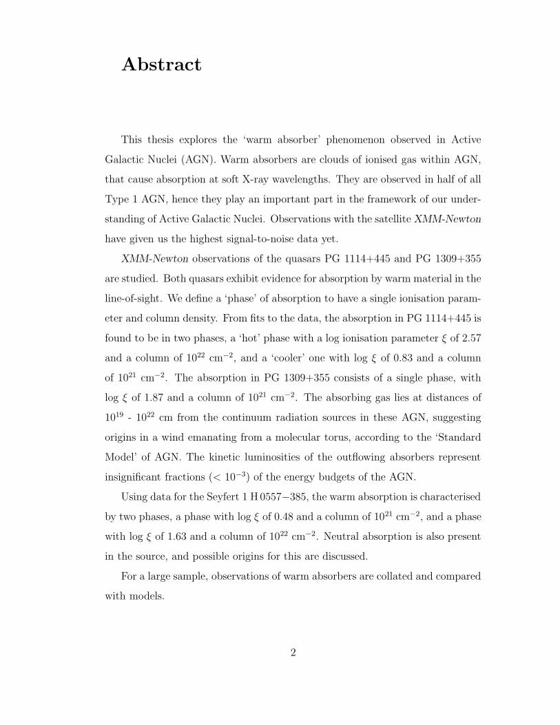
Abstract
This thesis explores the ‘warm absorber’ phenomenon observed in Active
Galactic Nuclei (AGN). Warm absorbers are clouds of ionised gas within AGN,
that cause absorption at soft X-ray wavelengths. They are observed in half of all
Type 1 AGN, hence they play an important part in the framework of our under-
standing of Active Galactic Nuclei. Observations with the satellite XMM-Newton
have given us the highest signal-to-noise data yet.
XMM-Newton observations of the quasars PG 1114+445 and PG 1309+355
are studied. Both quasars exhibit evidence for absorption by warm material in the
line-of-sight. We define a ‘phase’ of absorption to have a single ionisation param-
eter and column density. From fits to the data, the absorption in PG 1114+445 is
found to be in two phases, a ‘hot’ phase with a log ionisation parameter ξ of 2.57
and a column of 1022 cm−2, and a ‘cooler’ one with log ξ of 0.83 and a column
of 1021 cm−2. The absorption in PG 1309+355 consists of a single phase, with
log ξ of 1.87 and a column of 1021 cm−2. The absorbing gas lies at distances of
1019 - 1022 cm from the continuum radiation sources in these AGN, suggesting
origins in a wind emanating from a molecular torus, according to the ‘Standard
Model’ of AGN. The kinetic luminosities of the outflowing absorbers represent
insignificant fractions (< 10−3) of the energy budgets of the AGN.
Using data for the Seyfert 1 H0557−385, the warm absorption is characterised
by two phases, a phase with log ξ of 0.48 and a column of 1021 cm−2, and a phase
with log ξ of 1.63 and a column of 1022 cm−2. Neutral absorption is also present
in the source, and possible origins for this are discussed.
For a large sample, observations of warm absorbers are collated and compared
with models.
2
Contents
List of Figures 4
1 Introduction 11
1.1 Discovery of AGN . . . . . . . . . . . . . . . . . . . . . . . . . . . 11
1.2 What is an AGN? . . . . . . . . . . . . . . . . . . . . . . . . . . . 12
1.3 Classes of AGN . . . . . . . . . . . . . . . . . . . . . . . . . . . . 13
1.4 AGN Spectra . . . . . . . . . . . . . . . . . . . . . . . . . . . . . 17
1.4.1 Broad-band Spectra . . . . . . . . . . . . . . . . . . . . . 17
1.4.2 X-ray Spectra . . . . . . . . . . . . . . . . . . . . . . . . . 19
1.5 Absorption . . . . . . . . . . . . . . . . . . . . . . . . . . . . . . . 21
1.5.1 Cold absorption . . . . . . . . . . . . . . . . . . . . . . . . 21
1.5.2 Warm absorption . . . . . . . . . . . . . . . . . . . . . . . 21
1.5.3 The origins of warm absorbers . . . . . . . . . . . . . . . . 24
1.5.4 Warm absorbers in Quasars and Seyfert AGN . . . . . . . 25
1.5.5 Where are warm absorbers located in AGN? . . . . . . . . 27
1.5.6 UV and X-ray warm absorbers . . . . . . . . . . . . . . . . 28
1.6 The XMM-Newton observatory . . . . . . . . . . . . . . . . . . . 29
1.6.1 Pile-up . . . . . . . . . . . . . . . . . . . . . . . . . . . . . 33
1.6.2 Filters and window modes . . . . . . . . . . . . . . . . . . 33
2 PG 1114+445 and PG 1309+355 35
2.1 XMM-Newton observations . . . . . . . . . . . . . . . . . . . . . 36
3

CONTENTS 4
2.2 Initial fitting . . . . . . . . . . . . . . . . . . . . . . . . . . . . . . 37
2.2.1 Models including warm absorbers . . . . . . . . . . . . . . 42
2.2.2 The case of PG 1114+445 . . . . . . . . . . . . . . . . . . 42
2.2.3 The case of PG 1309+355 . . . . . . . . . . . . . . . . . . 46
2.3 Discussion . . . . . . . . . . . . . . . . . . . . . . . . . . . . . . . 47
2.3.1 Distances, filling factors and densities of the absorbers . . 49
2.3.2 Outflow and accretion rates . . . . . . . . . . . . . . . . . 50
2.3.3 Associated UV and X-ray absorber? . . . . . . . . . . . . . 52
2.3.4 Where is the warm absorber coming from? . . . . . . . . . 52
2.3.5 Comparison with other AGNs . . . . . . . . . . . . . . . . 56
2.4 Conclusion . . . . . . . . . . . . . . . . . . . . . . . . . . . . . . . 57
3 The Seyfert 1 AGN H 0557-385 59
3.1 Fits to the EPIC data . . . . . . . . . . . . . . . . . . . . . . . . 61
3.2 Fits to the RGS data . . . . . . . . . . . . . . . . . . . . . . . . . 67
3.3 Discussion . . . . . . . . . . . . . . . . . . . . . . . . . . . . . . . 69
3.3.1 Where did the warm absorbers originate? . . . . . . . . . . 74
3.3.2 Comparison with other AGN . . . . . . . . . . . . . . . . . 74
3.3.3 Where is the neutral gas component? . . . . . . . . . . . . 76
3.4 Conclusion . . . . . . . . . . . . . . . . . . . . . . . . . . . . . . . 77
4 Discussion 79
4.0.1 Connection with X-ray and UV absorbers . . . . . . . . . 79
4.0.2 Where can we place the warm absorbers? . . . . . . . . . . 81
4.0.3 A torus origin for warm absorbers? . . . . . . . . . . . . . 81
5 Conclusions 87
Bibliography 89

List of Figures
1.1 Images of NGC 4261 . . . . . . . . . . . . . . . . . . . . . . . . . 15
1.2 The Unified AGN model . . . . . . . . . . . . . . . . . . . . . . . 16
1.3 Mean Spectral Energy distributions from quasars . . . . . . . . . 17
1.4 Broad-band spectrum of IC 4329A demonstating reflection. . . . . 20
1.5 RGS Spectra of IRAS 13349+2438 . . . . . . . . . . . . . . . . . 22
1.6 Ionic abundance of oxygen. . . . . . . . . . . . . . . . . . . . . . . 23
1.7 Ionic abundance of iron. . . . . . . . . . . . . . . . . . . . . . . . 23
1.8 Ionisation cone diagram of the Seyfert 2 NGC 1068 . . . . . . . . 26
1.9 Quantum Efficiency of the pn CCD . . . . . . . . . . . . . . . . . 32
1.10 Quantum Efficiency of the MOS CCD . . . . . . . . . . . . . . . . 32
2.1 PG 1114+445: Power law fit. . . . . . . . . . . . . . . . . . . . . 38
2.2 PG 1114+445: Fit with single warm absorber. . . . . . . . . . . . 38
2.3 PG 1114+445: Fit with two warm absorbers. . . . . . . . . . . . . 39
2.4 PG 1114+445: Fit with two warm absorbers and iron Kα line. . . 39
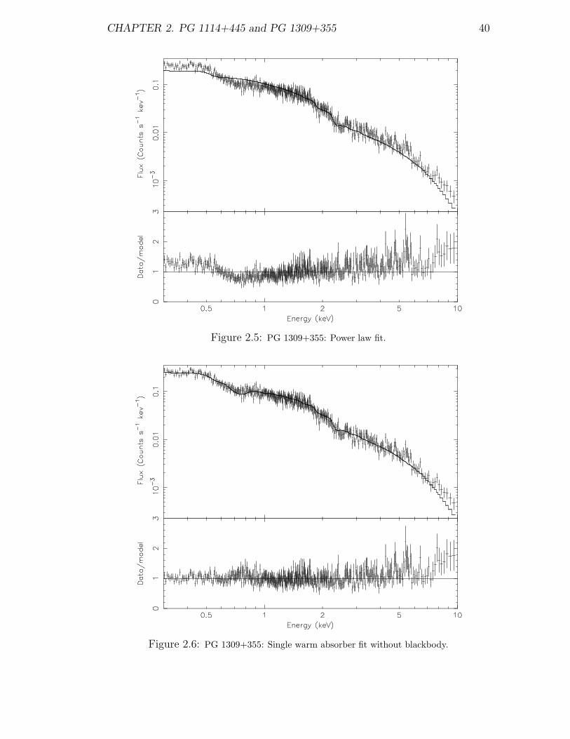
2.5 PG 1309+355: Power law fit. . . . . . . . . . . . . . . . . . . . . 40
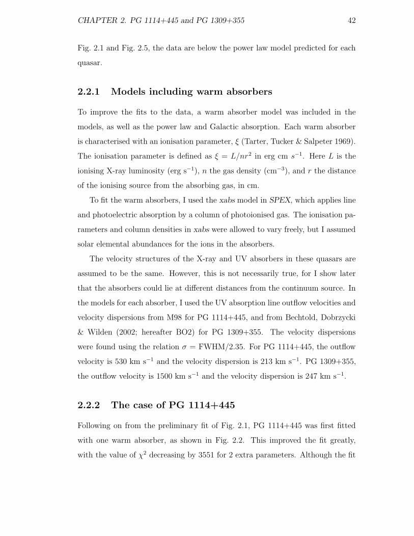
2.6 PG 1309+355: Single warm absorber fit without blackbody. . . . 40
2.7 PG 1309+355: Single warm absorber fit with blackbody. . . . . . 41
2.8 PG 1309+355: Single warm absorber fit with blackbody and iron
Kα line. . . . . . . . . . . . . . . . . . . . . . . . . . . . . . . . . 41
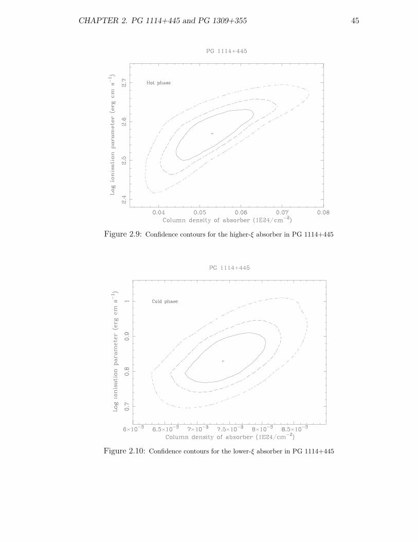
2.9 Confidence contours for the higher-ξ absorber in PG 1114+445 . . 45
2.10 Confidence contours for the lower-ξ absorber in PG 1114+445 . . 45
5

LIST OF FIGURES 6
2.11 Confidence contours for the absorber in PG 1309+355 . . . . . . . 46
2.12 Warm absorber models plotted at high resolution. . . . . . . . . . 48
3.1 H0557−385: Power law fit. . . . . . . . . . . . . . . . . . . . . . . 62
3.2 H0557−385: Fit with one warm absorber. . . . . . . . . . . . . . 62
3.3 H0557−385: Fit with two warm absorbers. . . . . . . . . . . . . . 63
3.4 H0557−385: Fit with two warm absorbers and neutral absorption. 63
3.5 H0557−385: Fit with two warm absorbers, neutral absorption and
iron Kα line. . . . . . . . . . . . . . . . . . . . . . . . . . . . . . . 64
3.6 H0557−385: Fit with two warm absorbers, neutral absorption and
reflection. . . . . . . . . . . . . . . . . . . . . . . . . . . . . . . . 64
3.7 The RGS spectrum of H0557−385, plotted with the best-fit EPIC
model. . . . . . . . . . . . . . . . . . . . . . . . . . . . . . . . . . 70
3.8 The RGS spectrum of H0557−385, with the best-fit model. . . . . 71
3.9 The RGS best-fit model for H 0557−385 . . . . . . . . . . . . . . 71
3.10 Comparison of IRAS 13349+2438, NGC 3783, and H0557−385. . 72
4.1 Log ξ versus log Lbol . . . . . . . . . . . . . . . . . . . . . . . . . 80
4.2 Log NHtotal versus log Lbol . . . . . . . . . . . . . . . . . . . . . . 80
4.3 Ionising luminosity, versus log of product of ionisation parameter
and column density, for 14 AGN. . . . . . . . . . . . . . . . . . . 83
4.4 Volume filling factors from this work plotted versus those derived
from Blustin et al (2005). . . . . . . . . . . . . . . . . . . . . . . 85
List of Tables
2.1 Observation details for PG 1114+445 and PG 1309+355 . . . . . 36
2.2 Power law and warm absorber parameters for PG 1114+445 and
PG 1309+355 . . . . . . . . . . . . . . . . . . . . . . . . . . . . . 43
2.3 X-ray and UV absorber line equivalent widths for PG 1114+445
and PG 1309+355. . . . . . . . . . . . . . . . . . . . . . . . . . . 53
2.4 A comparison of AGN warm absorber parameters. . . . . . . . . . 58
3.1 Observation details for H 0557−385. . . . . . . . . . . . . . . . . . 60
3.2 Parameters of fits to the combined EPIC data for H 0557−385. . . 66
3.3 Parameters of fits to the RGS and EPIC data of H 0557−385. . . 69
3.4 Comparison of warm absorber parameters for the type 1 AGN
NGC 3783, IRAS 13349+243 and H0557−385. . . . . . . . . . . . 75
4.1 Comparison of volume filling factors between this work and those
of Blustin et al (2005). . . . . . . . . . . . . . . . . . . . . . . . . 86
7

Acknowledgements
There are many people whom I have consulted for help during the writing of
this thesis; I’m sure you know who you all are!
My greatest thanks goes to my supervisors, Graziella Branduardi-Raymont
and Mat Page, for their guidance, help and the great amount of time they have
devoted to me, during my time at MSSL. It has been a pleasure to know such
marvellous people. I have benefited greatly from Graziella’s vast stores of knowl-
edge, and also her perfect command of the English languge which has shamed my
own schoolgirl grammar on many occasions. Similarly I have learnt much from
the huge amounts of time and effort Mat has devoted to me; I believe his sarcasm
has done me no lasting damage, and I hope sincerely he will discover there are
more culinary delights to be had than pot noodles.
I have also taken up a great deal of time from Alex Blustin and Rhaana
Starling, whom I thank deeply for their help and friendship. Thanks also to
Catherine Brocksopp, Nicola Loaring, Gavin Ramsay and Roberto Soria for being
great friends and colleagues.
I am pleased to have made the friendship of so many great people in the church
and village of Holmbury St.Mary, a definitive quintessential English village; their
interest in the work of MSSL has been inspiring. I also owe a great deal to
Mumsy, and her alarming ability to predict the future, generally quite useful but
especially so in times of crisis. I thank the Rev. Pam Robson for being a great
mentor, and Anne Payne, Annika Lohstroh and David Folkerd for their support
in finishing the thesis.
I would also like to thank Stephen Coulson and his family for their immense
hospitality towards me during my first year in Surrey (and in England, for that
matter.)
I am grateful to PPARC for financial support for the last 3 years.
I acknowledge initial guidance from the late Liz Puchnarewicz, an enthusiastic
astronomer who introduced me to PG quasars and, amongst other things, refined
my soul with fire. I doubt I will meet her like again.
Diolch yn fawr a iechyd da!
This work is based on observations obtained with XMM-Newton, an ESA sci-
ence mission with instruments and contributions directly funded by ESA Member
States and the USA (NASA). This research has made use of the NASA/IPAC Ex-
tragalactic Database (NED) which is operated by the Jet Propulsion Laboratory,
California Institute of Technology, under contract with the National Aeronau-
tics and Space Administration. This research has also made use of the SIMBAD
database, operated at CDS, Strasbourg, France.
The copyright of this thesis rests with the author and no quotation from it or
information derived from it may be published without the prior written consent
of the author.

When I consider thy heavens,
the work of thy fingers,
the moon and the stars, which thou hast
ordained;
What is man, that thou art mindful of him?
And the son of man, that thou visitest him?
Psalm 8

Chapter 1
Introduction
1.1 Discovery of AGN
AGN have fascinated astronomers for about a century now. But what are the
historical milestones that have led to the discovery of this most powerful class of
galaxies?
The first optical spectrum of an AGN was taken of NGC 1068 in 1908 (Fath
1909). Even then, emission lines were noted in the spectrum. Very soon after,
a higher-quality spectrum showed that the lines are resolved and have widths of
hundreds of km s−1. In 1926, in a study of extragalactic nebulae, Edwin Hubble
noted strong emission-line spectra of three galaxies: NGC 1068, NGC 4051 and
NGC 4151 (Hubble 1926). In 1943, Carl Seyfert was the first to identify a class
of spiral galaxies with bright, compact nuclei. Seyfert found that the optical
spectra of these bright galaxies have strong nuclear emission lines, and these are
now known as Seyfert galaxies.
In the 1960s, the apparent ‘stars’ 3C 273 and 3C 64, both strong radio emit-
ters, were measured to be at the then-huge redshifts of 0.158 and 0.367 respec-
tively. Dubbed quasi-stellar radio sources, later shortened to quasars, it was
realised that sources of this type all have large redshifts, broad emission lines and
11

CHAPTER 1. Introduction 12
are variable.
Astronomers have tried to account for the different properties of AGN by
invoking a unified model that can explain them all. First I describe the properties
of AGN, then I review the classes of AGN that have been identified.
1.2 What is an AGN?
Astronomers believe that at the centres of AGN there reside supermassive black
holes, with masses of millions of solar masses. They are immensely powerful,
capable of generating huge amounts of energy (> 1047 erg s−1), and they emit
radiation across practically the whole electromagnetic spectrum.
In the 1960s, the huge distances that quasars are at was first realised, im-
plying that they must have very high luminosities. It was suggested that such
luminosities could be produced by the efficient conversion of gravitational poten-
tial energy released by gases falling onto a black hole, into radiation by friction
in the accretion disk (e.g. Lynden-Bell 1969). Friction in the disk causes it to be-
come very hot (∼ 105-106 K) to the extent that it emits large amounts of X-rays.
Other effects are relativistic jets, boosted out along the disk’s axis.
Black holes can be spinning or not; spinning black holes are called Kerr black
holes, and non-spinning black holes are called Schwarzschild black holes. The
radius of the last stable orbit before material is sucked into a Kerr black hole is
2GM/c2, where G is the gravitational constant, M is the black hole mass and c
is the speed of light. For a Schwarzschild black hole the last stable orbit has a
radius equal to 6GM/c2.
The physical structure of AGN is now quite well understood. Starting at the
centre and moving out, we have the black hole, and the hot accretion disk, which
is of scales of light days. Then we have the broad-line region (BLR) clouds, on
scales of hundreds of light days. The BLR clouds are whirling around rapidly as
they are quite close in to the AGN, and yield optical emission lines with widths

CHAPTER 1. Introduction 13
of thousands of km s−1. They also have high densities, with electron densities 109
cm−3 or higher. Further out is the torus. This is an optically thick doughnut-
shaped ring of cold gas and dust that surrounds the central source, and is scales
of parsecs across. The narrow-line region (NLR) clouds, on scales of hundreds
of parsecs, are much further from the AGN and so do not whirl round quite as
fast as those of the BLR; the NLR optical emission lines have widths of hundreds
of km s−1, and can be resolved. The NLR clouds are low-density ionised gas
(electron densities 103-106 cm−3).
Lastly we have radio jets, which can extend to Mpc scales. Jets of relativis-
tic particles and magnetic fields are responsible for the radio emission: this is
thought to be due to synchrotron radiation of high energy electrons spiralling
along magnetic fields. Whether an AGN is radio-loud or radio-quiet is defined by
the strength of the jet radio emission, if present at all. Fanaroff & Riley (1974)
found that extended radio structures can be divided into two separate luminosity
classes.
Images of the torus and radio jet in the galaxy NGC 4261 are shown in Fig. 1.1.
1.3 Classes of AGN
The classification of AGN according to their observational properties has evolved
throughout the decades, as better instrumentation has become available and fea-
tures could be resolved to a higher degree.
The two types of AGN studied in this thesis are quasars and Seyfert galaxies.
First discovered optically (Seyfert 1943), Seyferts can be classified as either type
1 or type 2, depending on the widths of their optical emission lines: some AGN
were seen to have optical emission lines with widths up to thousands of km s−1
(Seyfert 1s) whereas others have widths of only hundreds of km s−1 (Seyfert 2s).
These days, the term ‘quasar’ refers to both radio-loud and radio-quiet sources,
although only ∼ 10 % of quasars are radio-loud.
CHAPTER 1. Introduction 14
Another class of AGN is BL Lacs. Greatly studied in the 1960’s and 1970’s,
a characteristic of these objects is the absence of strong absorption or emission
lines in their spectra. They are also polarised, variable and radio-loud; they are
thought to be radio galaxies with the radio jets viewed pole-on.
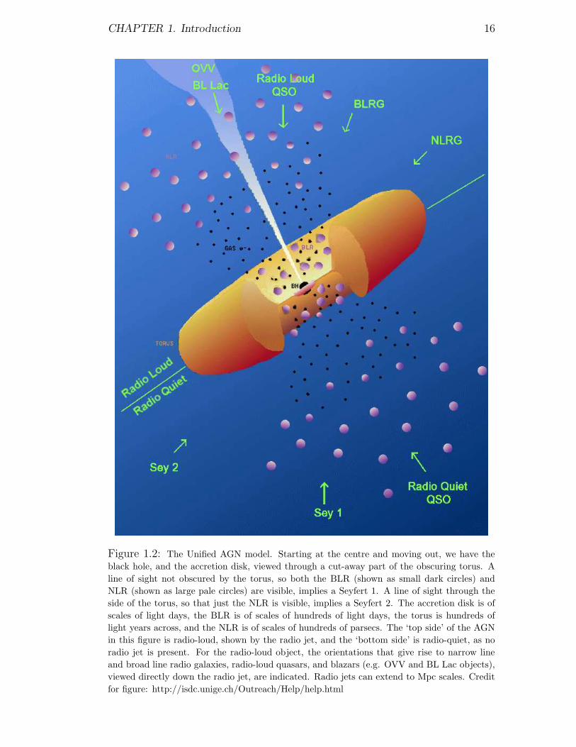
The reason for the dichotomy between Seyfert 1s and Seyfert 2s is explained
by the ‘Unified Model’ for AGN (Antonucci 1993; see Fig. 1.2). The dichotomy
is believed to arise from the obscuration of the central continuum source by
the torus, an optically thick doughnut-shaped ring of cold gas and dust that
surrounds the central source. Crucial evidence for the Unified model was found
by Antonucci & Miller (1985), who discovered a hidden Seyfert 1 nucleus in the
Seyfert 2 NGC 1068, by polarisation measurements of continuum and broad line
photons, scattered by electrons that lie above the torus. If we are looking directly
at the central source, then no obscuration is present and we will observe both the
broad and narrow line regions (Seyfert 1s); if we are looking through the torus,
then we will only observe the narrow line region (NLR) clouds which lie outside
the torus, and the broad line region (BLR) will be obscured (Seyfert 2s). As
mentioned earlier, the BLR clouds are close to the AGN, their optical emission
lines have widths of thousands of km s−1 and are produced at high densities
(electron densities 109 cm−3 or higher). The NLR clouds are much further from
the AGN, and have line widths of hundreds of km s−1. They consist of low-
density ionised gas (electron densities 103-106 cm−3). The NLR is shaped by the
torus into ‘ionisation cones’, and the shape can be discerned in Seyfert 2 AGN
as they are observed from the side (e.g. Capetti et al 1999). The best example
of ionisation cones is seen in NGC 1068 (Pogge 1988). A range of intermediate
types between Seyfert 1s and 2s also exist, dependent on the ratio of the broad
to narrow line strength. Maiolino & Rieke (1995) find that Seyfert 2s are 4 times
more numerous than Seyfert 1s.
Fig. 1.2 shows what is currently believed to be the AGN model that explains
the many different observed types.

CHAPTER 1. Introduction 15
Figure 1.1: Images of the galaxy NGC 4261. LHS: an optical image (white) is su-
perimposed on a radio image (orange). The central source and radio jets are very clear.
RHS: a close-up of the central source reveals the gas and dust torus. Credit for figure:
http://hubblesite.org/newscenter/newsdesk/archive/releases/1992/27/image/b
The most important difference between Seyferts and quasars is the amount of
radiation from the central source. In optical wavelengths the luminosity typically
emitted by a Seyfert central source is similar to that emitted by the sum of the
galaxy stars, but in the case of quasars, the luminosity from the source is greater
than that of the stars by a factor of at least 100. Hence, in Seyfert galaxies the
host galaxy can be seen, but in quasars, host galaxies are difficult to see because
of the glare from the quasar. At X-ray wavelengths, the measure usually used is
the 2-10 keV luminosity; a quasar has typically L2−10 > 1044 erg s−1 and a Seyfert
galaxy has L2−10 < 1044 erg s−1 (e.g. Loaring et al 2003).
CHAPTER 1. Introduction 16
Figure 1.2: The Unified AGN model. Starting at the centre and moving out, we have the
black hole, and the accretion disk, viewed through a cut-away part of the obscuring torus. A
line of sight not obscured by the torus, so both the BLR (shown as small dark circles) and
NLR (shown as large pale circles) are visible, implies a Seyfert 1. A line of sight through the
side of the torus, so that just the NLR is visible, implies a Seyfert 2. The accretion disk is of
scales of light days, the BLR is of scales of hundreds of light days, the torus is hundreds of
light years across, and the NLR is of scales of hundreds of parsecs. The ‘top side’ of the AGN
in this figure is radio-loud, shown by the radio jet, and the ‘bottom side’ is radio-quiet, as no
radio jet is present. For the radio-loud object, the orientations that give rise to narrow line
and broad line radio galaxies, radio-loud quasars, and blazars (e.g. OVV and BL Lac objects),
viewed directly down the radio jet, are indicated. Radio jets can extend to Mpc scales. Credit
for figure: http://isdc.unige.ch/Outreach/Help/help.html

CHAPTER 1. Introduction 17
µ10 cm 1 mm 10 m 1000Å 1.2 keV
Figure 1.3: Mean spectral energy distributions, normalised at 1.25µm, for radio-loud (dashed
line) and radio-quiet (solid line) quasars. Figure from Elvis et al (1994).
1.4 AGN Spectra
1.4.1 Broad-band Spectra
AGN spectra span from the far infrared to hard X-rays, with almost equal power
per decade of frequency; radio-loud objects also emit significantly in the radio
part. Some of the processes which give rise to the different parts are thermal,
i.e. radiation from particles with a Maxwellian velocity distribution. The rest are
non-thermal, i.e. radiation from particles whose velocities are not described by a
Maxwell-Boltzmann distribution; an example of this is particles that create syn-
chrotron powerlaw spectra, as the distribution of kinetic energy of these particles
must also be a powerlaw.
A mean spectral energy distribution for quasars is shown in Fig. 1.3. The
radio-loud AGN are seen to lie above the radio-quiet AGN at the hardest X-rays
and in the radio.
CHAPTER 1. Introduction 18
At energies below 1 keV, there are 2 gaps in the spectra where data are not
available; one of these is in the extreme ultraviolet (EUV) part of the spectrum
(∼ 1016 Hz) and the other is in the millimetre-wavelength regime.
The gap in the EUV is due mainly to the opacity of the ISM in our own Galaxy.
The gap at longer wavelengths, the ‘millimetre gap’, occurs for a few reasons.
Between ∼ 1 and 300 µm, water vapour absorption in the Earth’s atmosphere
makes it opaque to infrared and longer wavelengths; however up to ∼ 20 µm there
are some transparent atmospheric windows. For wavelengths longer than ∼ 300
µm, the opacity of the Earth’s atmosphere is such that ground-based observations
can be done from some very high mountain sites; however, there is a shortage of
data due to a lack of sensitive detectors.
The UV/Optical Band
The main feature of the UV/optical spectra of AGN is the ‘big blue bump’, (e.g.
Shang et al 2005), believed to arise from thermal emission in the range 105±1
K. It covers the wavelength range from ∼ 4000 A to at least 1000 A . It is not
known how strong the big blue bump is in the EUV, as our galaxy becomes almost
opaque at wavelengths between 912 A and ∼ 100 A due to absorption by neutral
hydrogen.
The big blue bump is generally thought to be thermal emission from an op-
tically thick, geometrically thin accretion disk. As the disk has a decreasing
temperature gradient, moving radially out from the centre, the resulting emis-
sion spectrum is roughly a multi-blackbody spectrum.
The Infrared Band
AGN infrared continua are described by a broad, smooth bump between the wave-
lengths of ∼ 2 - 100 µm. The emission can be thermal or non-thermal in origin.
A great deal, if not all, of the infrared continuum is thermal emission from dust,
illuminated by the AGN. The emission is generally comparable in strength to the

CHAPTER 1. Introduction 19
optical - UV, and is far too broad to be explained by a single-temperature grey-
body; a range of dust temperatures ∼ 50 - 500 K are required. A local minimum
at ∼ 1 µm implies a thermal emission mechanism in the near infrared. At these
wavelengths, thermal emission would require temperatures of ∼ 2000 K; this is
believed to be emission from the dust closest to the nuclear source (∼ 0.1 pc) e.g.
Barvainis (1987).
1.4.2 X-ray Spectra
A main characteristic of AGN is that they emit across the whole electromagnetic
spectrum; multiwavelength observations, e.g. Brocksopp et al (2005), are impor-
tant for constructing a picture of how AGN work as a whole. The X-ray band is
extremely important as it allows us to investigate the regions closest to the black
hole.
AGN are powered by accretion, but the accretion disk is too cool to produce
the observed X-rays. To explain this, a ‘corona’ (Haardt & Maraschi 1991), is
invoked, that consists of a tenuous gas of hot electrons. It is postulated to lie close
to the accretion disk. UV photons from the accretion disk are upscattered several
times by the electrons in the corona and boosted in energy through the inverse
Compton effect. The hot electrons in the corona have a powerlaw distribution
of energy; this gives rise to the power law shape of the continuum, in which the
number of photons per unit energy E is proportional to E−Γ, Γ being the photon
index.
Sometimes we see a reflection component, which peaks between about 20 and
50 keV. The shape of this reflection ‘hump’ is due to two mechanisms. One is
Compton down-scattering of energetic photons, which recoil off lower-energy elec-
trons in comparatively cold material, such as the outer parts of the accretion disk
or the torus. In doing so they lose energy, resulting in a spectral fall-off at high
energies (E > 50 keV). At lower-energies (< 10 keV), the photoelectric absorption

CHAPTER 1. Introduction 20
Figure 1.4: A broad-band spectrum of IC 4329A, denoted as crosses. The dashed curve gives
the incident spectrum, the dotted curve shows the reflection component including a fluorescent
Fe Kα line, and the solid line denotes the sum. Figure from Magdziarz & Zdziarski (1995).
cross-section is much larger than the cross-section for Compton scattering in cool
material, so photoelectric absorption prevents reflection. These aspects combine
to create the hump-like feature.
A spectrum of the Seyfert 1.2 IC 4329A is shown in Fig. 1.4. Also shown in
this Figure are the best-fit model components that demonstrate how the shape of
the spectrum arises. The absorbed incident spectra is distorted by the underlying
reflection.
Often an iron Kα line at 6.4 keV, formed by fluorescence, is present; one is
clearly present in Fig. 1.4. Fluorescence is a process whereby an atom’s inner-
shell electron is knocked out by a high-energy photon; following this, two things
can happen. An M-shell electron can drop down and fill the vacancy, with the
emission of a photon; or, as the ion is in an excited state, an outer shell electron
can be emitted. The latter event is known as the Auger effect, and the ejected
electron is known as an Auger electron. The probability that a photon is emitted
rather than an Auger electron is known as the fluoresence yield; iron has the
highest fluoresence yield, of 34 %. Iron Kα lines are often present in AGN and in
particular are present in all objects studied in this thesis. A review of reflection

CHAPTER 1. Introduction 21
and AGN iron lines is given in Fabian et al (2000).
In most sources an excess of emission above the extrapolated power law, below
∼ 1 keV in the soft X-ray band, is seen; this is known as the ‘soft excess’. One
theory for this component is that it is an extension of the big blue bump, seen in
the UV, that comes from the accretion disk.
1.5 Absorption
1.5.1 Cold absorption
Cold absorption from our own Galaxy is always present in X-ray spectra, but
sometimes there is additional cold absorption. This could originate in a variety
of locations, e.g. the host galaxy of the AGN or cold material near the AGN. Such
additional cold absorption occurs in the spectra of H 0557−385 and is discussed
in Chapter 3, but does not occur in PG 1114+445 or PG 1309+355.
1.5.2 Warm absorption
Warm absorbers are clouds of ionised gas intrinsic to AGN. They were first
suggested by Halpern (1984) to explain Einstein data of the quasar MR 2251-
178. They are dubbed ‘warm’ absorbers as they imply gas at temperatures of
∼ 104 − 105 K (Krolik & Kriss 2001); the gas is photoionised, not collisionally
ionised. High resolution observations of warm absorbers have shown that they
are outflowing (e.g. Kaastra et al 2000, Reeves et al 2003). The abundances of
different elements can also be derived from spectroscopy (e.g. Blustin et al 2002).
The spectral sign of a warm absorber is a deficit of counts in the soft X-ray
part of the spectrum with respect to the extrapolation of a power law fit carried
out at energies above ∼ 2 keV.
Warm absorbers were found to be of importance in the study of AGN following
a study of 24 type 1 AGN (Reynolds 1997), which showed them to be present
CHAPTER 1. Introduction 22
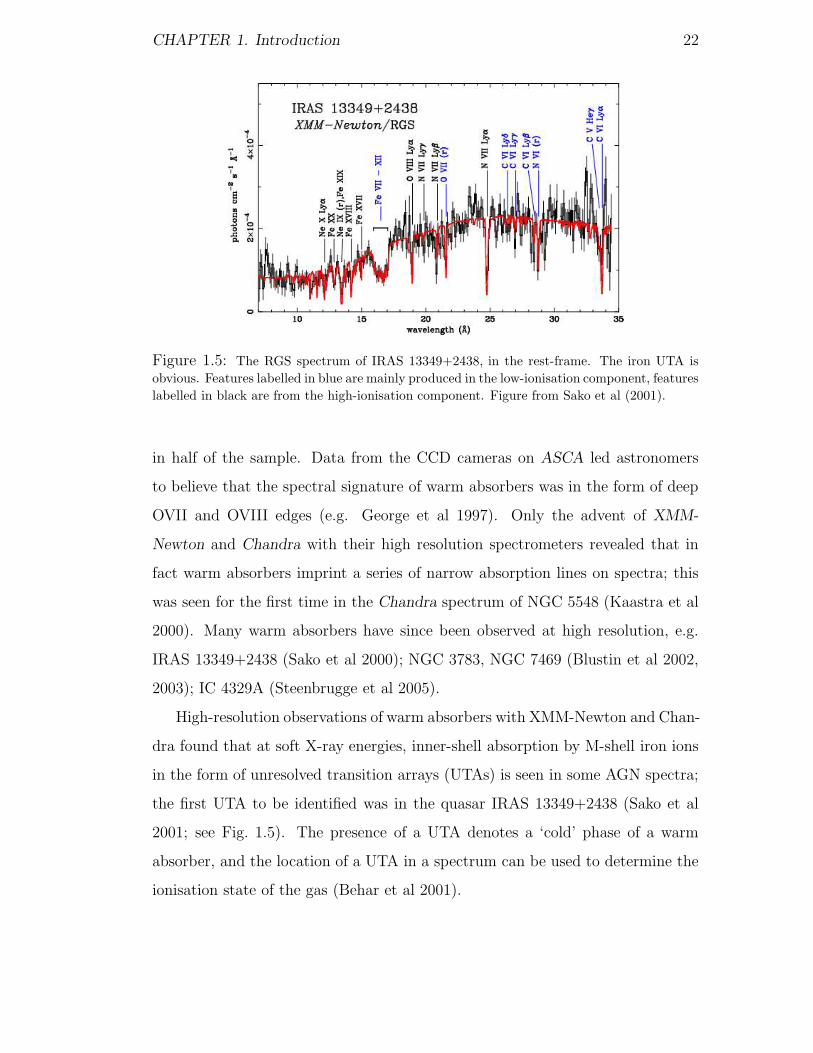
Figure 1.5: The RGS spectrum of IRAS 13349+2438, in the rest-frame. The iron UTA is
obvious. Features labelled in blue are mainly produced in the low-ionisation component, features
labelled in black are from the high-ionisation component. Figure from Sako et al (2001).
in half of the sample. Data from the CCD cameras on ASCA led astronomers
to believe that the spectral signature of warm absorbers was in the form of deep
OVII and OVIII edges (e.g. George et al 1997). Only the advent of XMM-
Newton and Chandra with their high resolution spectrometers revealed that in
fact warm absorbers imprint a series of narrow absorption lines on spectra; this
was seen for the first time in the Chandra spectrum of NGC 5548 (Kaastra et al
2000). Many warm absorbers have since been observed at high resolution, e.g.
IRAS 13349+2438 (Sako et al 2000); NGC 3783, NGC 7469 (Blustin et al 2002,
2003); IC 4329A (Steenbrugge et al 2005).
High-resolution observations of warm absorbers with XMM-Newton and Chan-
dra found that at soft X-ray energies, inner-shell absorption by M-shell iron ions
in the form of unresolved transition arrays (UTAs) is seen in some AGN spectra;
the first UTA to be identified was in the quasar IRAS 13349+2438 (Sako et al
2001; see Fig. 1.5). The presence of a UTA denotes a ‘cold’ phase of a warm
absorber, and the location of a UTA in a spectrum can be used to determine the
ionisation state of the gas (Behar et al 2001).

CHAPTER 1. Introduction 23
Figure 1.6: The ionic abundance for oxygen, versus ξ, within a photoionised plasma. The
curves from left to right correspond to increasingly ionised oxygen, from O I - O IX. Credit for
figure: Jelle Kaastra, SRON.
Figure 1.7: The ionic abundance for iron, versus ξ, within a photoionised plasma. The curves
from left to right correspond to increasingly ionised iron, from Fe I - Fe XXVII. Credit for
figure: Jelle Kaastra, SRON.
CHAPTER 1. Introduction 24
In most observations, it is found that more than one ‘phase’ of warm absorber
is present. Two phases were proposed for IRAS 13349+2438 (Sako et al 2000),
whereas Steenbrugge et al (2003) find three phases of warm absorber in NGC 5548.
We define a phase as gas at a particular ionisation parameter, ξ, and column
density. We define the ionisation parameter as ξ = L/nr2 in erg cm s−1 (Tarter
et al 1969). Here L is the ionising luminosity (erg s−1, taken to be the 1-1000
Rydberg luminosity), n the gas density (cm−3), and r the distance of the ionising
source from the absorbing gas, in cm.
Fig. 1.6 and Fig. 1.7 show the ionic abundances of oxygen and iron, respec-
tively, for a photoionised plasma. Both ions are important in AGN absorption
spectra, oxygen being highly abundant and contributing much absorption, and
iron forming a UTA if the ionisation parameter is in the right range. OVII is
most abundant at log ξ values of 1, whereas OVIII is most abundant nearer log
ξ values of 2. The ionisation parameters that lead to an M-shell UTA of iron (Fe
X - Fe XVI) are ∼ 0-2.
1.5.3 The origins of warm absorbers
There are currently two main theories for the origins of warm absorbers. One
explanation is a wind formed by photoionised evaporation from the inner edge of
the torus (Krolik & Kriss 2001), lying a few parsecs from the continuum source.
Reynolds (1997) suggests that ‘outer’ absorbers may be a radiatively driven dusty
wind from the torus; it could be ionised material on the inner edge of the torus,
driven by radiation pressure which would give it a conical shell-like structure.
Another possibility is a wind driven off the accretion disk. By analogy with
winds from hot stars, Castor, Abbott & Klein (1975) consider the force exerted on
stellar material as result of absorption and scattering of line radiation, thought
to be responsible for the outflow of material in massive hot stars. From the
concept that momentum is extracted most efficiently from the radiation field via

CHAPTER 1. Introduction 25
line opacity, Castor, Abbott & Klein (1975) show that a great number of lines
from many different elements contribute to the total force. Applying the concept
of such a wind to AGN, Proga et al (2000) find that a disk accreting around a
108 M black hole can launch a wind at ∼ 1016 cm from the central engine. Elvis
(2000) finds that an accretion disk wind, viewed at different angles, will explain
the many varieties of absorption features seen in quasars.
As for the geometry of warm absorbers, recent high-resolution X-ray observa-
tions of the Seyfert 2 NGC 1068 (Kinkhabwala et al 2002; Brinkman et al 2002)
suggest that in this source we are viewing the warm absorber in emission, in
the shape of an ionisation cone. Kinkhabwala et al (2002) find that the column
densities and ionisation parameters observed in Seyfert 2s are consistent with
those found in warm absorbers in Seyfert 1 AGN. Fig. 1.8 shows a cartoon of the
ionisation cone of NGC 1068.
1.5.4 Warm absorbers in Quasars and Seyfert AGN
Warm absorbers are common in Seyferts: in the study mentioned above of 24
type 1 AGN, of which 18 are Seyfert galaxies, half were found to have warm
absorbers (Reynolds 1997). However, they are far rarer in quasars. In a study
of 23 quasars, only one was found to display warm absorption (Laor 1997). So,
is there any physical difference in the warm absorbers observed in different types
of AGN?
Relativistic outflows have been reported for the quasars PG 0844+349 (Pounds
et al 2003a), PG 1211+143 (Pounds et al 2003b) and PDS 456 (Reeves et al 2003).
These authors find that the absorber can, in each case, be modelled with a single,
very high ionisation parameter, much higher than is usually found in quasars
or Seyferts; however, Kaspi et al (2004), using the same data, suggest that the
absorption lines in PG 1211+143 imply an outflow of just 3000 km s−1, instead
of 24,000 - 30,000 km s−1 as suggested by Pounds et al (2003b). But such fast

CHAPTER 1. Introduction 26
Figure 1.8: A cartoon of the ionisation cone of NGC 1068 (not to scale). The black dot
represents the central source. For a Seyfert 1, the ionisation cone comprising the warm absorber
is observed end-on as it absorbs the central source radiation. For a Seyfert 2, the torus (shown
as blobs either side of the central source, cut away to show the source) absorbs the radiation
from the central source, and the ionisation cone is seen in emission. Figure from Kinkhabwala
et al (2002).

CHAPTER 1. Introduction 27
outflows are by no means found in all quasar warm absorbers, so they are not
necessarily representative.
From a detailed study of the warm absorbers in 23 AGN, Blustin et al (2005)
find that bolometric luminosity is not correlated with average ionisation parame-
ter; neither is it correlated with total column. If PG 0844+349 and PG 1211+143
are ignored, then the average outflow speeds are not greatly correlated with bolo-
metric luminosity, column or average ionisation parameter. There seems to be no
defining difference between the warm absorbers seen in different types of AGN.
1.5.5 Where are warm absorbers located in AGN?
Locating the positions of warm absorbers in AGN has been found to be tricky.
At present, no definitive idea exists of where warm absorbers live in the structure
of AGN; Krolik & Kriss (2001) speculate that they could lie anywhere from
the broad-line region, to tens of parsecs out. Hence their origins are essentially
unconstrained, which is one of the motivations for the research in this thesis.
If a warm absorber is a wind from the inner edge of the torus (Krolik & Kriss
2001), then it will exist a few parsecs from the continuum source; on the other
hand, if it is a wind driven off the accretion disk, Proga et al (2000) find that it
can be launched at ∼ 1016 cm from the central engine.
The ionisation cone scenario suggested for the Seyfert 2 NGC 1068 (Kinkhab-
wala et al 2002; Brinkman et al 2002), which means we see the warm absorber in
emission in this type of galaxy, places it at the distance of the NLR of the AGN,
at hundreds of pc.
From their sample of 23 AGN, Blustin et al (2005) find that warm absorbers
are most likely to originate as outflows from the torus. For the absorber of
PG 1114+445, Mathur et al (1998) find the absorber eats into emission lines,
placing it outside the BLR; they put an upper limit of 4×1017 cm for the distance
of the absorber. However, from the 900ks Chandra observation of NGC 3783,
CHAPTER 1. Introduction 28
Netzer et al (2003) obtain lower limits of 3.2, 0.6 and 0.2 pc for the distances of
the three separate absorbers found.
1.5.6 UV and X-ray warm absorbers
It has been hypothesised for some time now that there are strong relations be-
tween X-ray and UV absorbers, or maybe even that they both have a common
origin. The evidence for this has been gathering ground recently.
Observationally, Mathur, Wilkes & Elvis (1998) model the absorption in
PG 1114+445 with a single UV and X-ray absorber. They found that the out-
flowing velocity of both the X-ray and UV absorbers is 530 km s−1, and that the
derived ion column densities from both absorbers agree.
Convincing evidence comes from the study by Crenshaw et al (1999), who
found that there is a 1:1 correlation of UV absorbers and X-ray absorbers. Their
study found that in most cases the UV absorbers are outflowing, as are the X-
ray absorbers; the cores of the strong absorption components are much deeper
than the continuum flux levels, which indicates that the absorption components
exist completely outside of the broad emission-line regions. From the sample it
is induced that the intrinsic absorbers cover a large part of the sky (≥ 50%) as
seen from the continuum source.
What processes take place for a wind to arise? Close in to the central source,
the gas is over-ionised and few atomic transitions are available, so electron scat-
tering prevails. This cannot drive a wind alone, and this ‘failed’ wind then acts
to screen the gas further out from the central source. In doing so, the ionisation
parameter is lowered; when it falls below a certain value, the number of tran-
sitions and the opacity rises very fast, making the radiation and line driving ∼1000 times stronger than just electron scattering, and a wind is formed. Most of
the UV and soft X-ray continuum is absorbed by the wind (Elvis 2004).
From hydrodynamical calculations of line-driven winds from AGN, Proga et al

CHAPTER 1. Introduction 29
(2000) find that local disk radiation can launch a disk wind, even in the presence
of strong ionising radiation from the central object. This central radiation may
cause the part of the flow to be over-ionised, and slow the wind down. The X-ray
opacity of the wind must be much higher than the UV opacity, in order to create
a fast wind. So that the stream is optically thin to the UV radiation but optically
thick to X-rays, a typical column density radially through the fast stream is a
few 1023 cm−2. For a disk accreting around a 108 M black hole, a wind can
be launched at ∼ 1016 cm from the central engine; then for a reasonable X-ray
opacity, the wind can be accelerated by the central UV radiation to velocities of
up to 15000 km s−1.
1.6 The XMM-Newton observatory
The XMM-Newton spacecraft (Jansen et al 2001) is the largest scientific satellite
ever launched by the European Space Agency. With a total effective area of ∼4500 cm2 (1500 cm2 at 1 keV per telescope, x 3 telescopes), it has much greater
sensitivity than Chandra (collecting area of 800 cm2 at 0.25 keV and 400 cm2 at
5 keV); in fact XMM-Newton has more than ten times the effective area than
Chandra at ∼ 6-7 keV, a very important energy band for the study of the K-
shell transitions of iron. In contrast, Chandra has higher spatial resolution, with
0.5′′ FWHM from the HRC (High Resolution Camera), compared to a spatial
resolution of 6′′ FWHM from the EPIC instruments on XMM-Newton.
Each of XMM-Newton’s three X-ray telescopes is made of 58 closely packed
mirror shells to get the highest effective area. Operating in a 48 hour eccentric
orbit, XMM-Newton provides uninterrupted observing capability for up to 40
hrs. The spacecraft houses three imaging X-ray instruments. At the primary
focus of the 3 telescopes, there are 3 EPIC (European Photon Imaging Camera)
CCD cameras. Two are EPIC MOS cameras (Turner et al 2001), employing
arrays of Metal-Oxide-Silicon (MOS) X-ray sensitive CCDs; one is an EPIC pn

CHAPTER 1. Introduction 30
camera (Struder et al 2001), with a pn CCD. They provide imaging and medium
resolution spectroscopy. Associated with the two telescopes with MOS cameras
are the high-resolution RGSs (Reflection Grating Spectrometers; den Herder et
al 2001). Both RGS chains incorporate an array of gold-coated reflection gratings
that deflect about half the light incident on them, whilst allowing the other half
to be transmitted to the primary focus where the MOS cameras are located. The
EPIC pn telescope has no gratings behind it, so the pn camera receives all the
X-ray flux. Co-aligned with the X-ray instruments is the optical monitor (Mason
et al 2001), a 30cm optical/ultraviolet telescope.
The spatial resolution of EPIC is such that the in-orbit measured Point Spread
Function half-energy width, within which half of the light from the telescopes is
focussed, is 15.2′′ for pn, 13.8′′ for MOS1 and 13.0′′ for MOS2. Later in this thesis
I extract spectra by selecting source photons within circles of radius 25-30′′. For
the EPIC instruments, 30′′ corresponds to ∼ 80% fraction encircled energy.
The EPIC cameras take imaging spectroscopy over the telescope’s field of
view (FOV) of 30 arcmin and in the energy range 0.15 to 15 keV, with moderate
spectral resolution (E/∆E ∼ 20-50). All the CCDs of the EPIC instruments
produce data in the form of event lists, that is, tables with one entry line per
received event, listing the positions at which the photons were registered, their
arrival times and their energies.
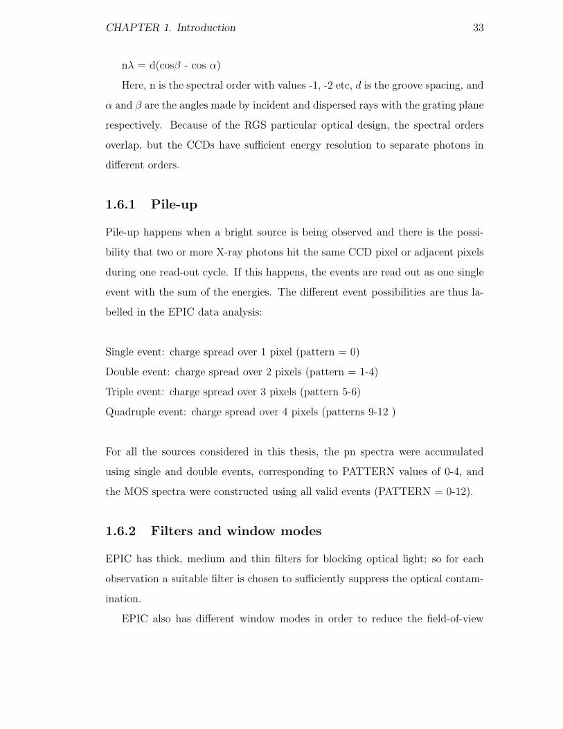
The MOS detectors are most efficient in the 1-5 keV range. As they only have
a 40-micron sensitive depth of silicon, the detectors are less responsive to hard
X-rays. Each MOS CCD consists of seven silicon chips, each made up of a matrix
of 600 x 600 pixels (1 pixel = 1.1′′).
The PN camera, with a 300-micron thickness of silicon, registers hard X-rays
better than the MOS camera. Also in contrast to the MOS camera, the PN
detector has a 400 x 400 pixel matrix of size 6 cm x 6 cm (1 pixel = 4.1′′).
One important practical difference between the MOS and pn cameras is their
time resolution. The pn has a much higher time resolution, as each pixel column
CHAPTER 1. Introduction 31
in the pn camera has its own readout node. In full-frame mode, the MOS reads
out in 2.6s, whereas for the pn, the parallel readout of channels enables the camera
to be operated quickly: in full-frame mode, only 73 ms are needed to acquire one
frame.
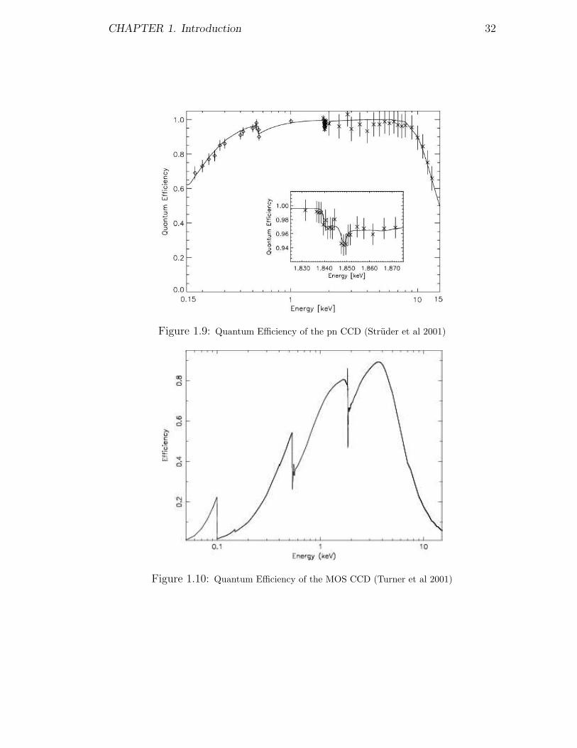
The type of illumination of the chips also affects the quantum efficiency (QE),
defined as the fraction of incident photons on the detector that generate an event
in the CCD. The QE differs between the MOS and pn CCDs: the QE of the pn
CCDs is higher than that of the MOS CCDs, see Fig. 1.9 and Fig. 1.10. As the pn
CCD is illuminated from the rear side (back-illuminated), which does not have
insensitive layers or coatings, the X-ray detection efficiency is extremely high and
homogeneous from the very low to the highest energies (over 90% from 0.5 to 10
keV).
The RGS is designed for high spectral resolution measurements in the soft X-
ray range, where the K-shell transitions of C, N, O, Ne Mg, Si, S and C, and also
the L-shell transitions of Fe are located. It allows detailed line diagnostics, and
from such measurements the density, temperature, ionisation state and chemical
composition of the sources observed can be determined. RGS has much higher
energy resolution (E/∆E ∼ 200-800 over an energy range 0.3-2.1 keV) than EPIC
(E/∆E ∼ 20-50, energy range of 0.1-15 keV).
The RGS spectrum is dispersed in wavelength so individual lines and line
profiles can be resolved. The reflection gratings are basically mirrors with many
tiny grooves on them. The gratings are covered with a gold layer and there are
600 grooves per millimeter. The light from the telescope grazes off the plates, and
diffraction occurs in the beams reflected from the grooves. For a given spectral
order, the angle of reflectance is greater for longer wavelengths, producing a
dispersed spectrum.
The X-rays dispersed into a spectrum are focussed on the two RGS cameras.
The position of an X-ray of wavelength λ on the CCD array is given by the
dispersion equation
CHAPTER 1. Introduction 32
Figure 1.9: Quantum Efficiency of the pn CCD (Struder et al 2001)
Figure 1.10: Quantum Efficiency of the MOS CCD (Turner et al 2001)
CHAPTER 1. Introduction 33
nλ = d(cosβ - cos α)
Here, n is the spectral order with values -1, -2 etc, d is the groove spacing, and
α and β are the angles made by incident and dispersed rays with the grating plane
respectively. Because of the RGS particular optical design, the spectral orders
overlap, but the CCDs have sufficient energy resolution to separate photons in
different orders.
1.6.1 Pile-up
Pile-up happens when a bright source is being observed and there is the possi-
bility that two or more X-ray photons hit the same CCD pixel or adjacent pixels
during one read-out cycle. If this happens, the events are read out as one single
event with the sum of the energies. The different event possibilities are thus la-
belled in the EPIC data analysis:
Single event: charge spread over 1 pixel (pattern = 0)
Double event: charge spread over 2 pixels (pattern = 1-4)
Triple event: charge spread over 3 pixels (pattern 5-6)
Quadruple event: charge spread over 4 pixels (patterns 9-12 )
For all the sources considered in this thesis, the pn spectra were accumulated
using single and double events, corresponding to PATTERN values of 0-4, and
the MOS spectra were constructed using all valid events (PATTERN = 0-12).
1.6.2 Filters and window modes
EPIC has thick, medium and thin filters for blocking optical light; so for each
observation a suitable filter is chosen to sufficiently suppress the optical contam-
ination.
EPIC also has different window modes in order to reduce the field-of-view

CHAPTER 1. Introduction 34
electronically to reduce the readout rate and hence improve the time resolution:
this increases the pile-up count-rate limit for bright sources (Struder et al 2001).
Chapter 2
PG 1114+445 and PG 1309+355
PG 1114+445 is a radio-quiet quasar that was listed in the Bright Quasar Survey
(BQS, Schmidt & Green 1983) and belongs to a subset of 23 quasars in the BQS
with z ≤ 0.4 and Galactic Nh ≤ 1.9×1020 cm−2 (Laor 1997). PG 1114+445 has a
redshift of 0.144 and Galactic Nh of 1.83×1020 cm−2 (Dickey & Lockman 1990).
The presence of a warm absorber in PG 1114+445 is well known. Using
ROSAT and ASCA data, George et al (1997) model the absorption in PG 1114+445
as OVII and OVIII edges, and determine the column density of the ionised gas
to be ∼ 2×1022 cm−2. Mathur et al (1998; hereafter M98) find that the absorber
lies outside the BLR, or is cospatial with it, and has a mass outflow rate of 1 M
yr−1.
As found by Reynolds (1997), significant absorption could occur for ∼ 50% of
lower-luminosity AGNs, wheras it is rare for quasars, occuring for less than 5% of
the subset of Laor (1997). Crenshaw et al (1999) find that there is a one-to-one
correlation of UV and X-ray absorbers in Seyfert galaxies; both X-ray and UV
absorption have been observed in PG 1114+445. The HST spectrum of M98
shows strong UV absorption lines blueshifted by ∼ 530 km s1 from the systemic
redshift of the quasar.
PG 1309+355 is a radio-intermediate AGN that was listed in the BQS. A
warm absorber has not been detected in this source prior to the XMM-Newton
35

CHAPTER 2. PG 1114+445 and PG 1309+355 36
Table 2.1: Galactic column densities and observation details. Obs. Date is Observation Date,
Gal. Nh is Galactic Nh in units of 1020cm−2 and Eff. Exp. Time is Effective Exposure Time.
Quasar Obs. Redshift Gal. Nh Eff. Exp. Time Count Rate
Date 1020 cm−2 (ks) (Counts s−1)
PG 1114+445 15.05.02 0.144 1.83 PN:37, MOS:42 PN:0.67, MOS:0.20
PG 1309+355 10.06.02 0.184 1.03 PN:23, MOS:29 PN:0.50, MOS:0.13
observation. PG 1309+355 lies at a redshift of 0.184 and has a Galactic Nh of
1.03×1020 cm−2 (Dickey & Lockman 1990).
2.1 XMM-Newton observations
PG 1114+445 and PG 1309+355 were observed with XMM-Newton (Jansen et al
2001) as part of the OM Guaranteed Time programme. The EPIC observations
of both objects were done using the thin filter, with the cameras in large window
mode.
Table 2.1 summarises the Galactic column densities (from Dickey & Lockman
1990), the redshifts (from L97), and observation details. The RGS data do not
contain enough counts for us to construct a useful spectrum for either quasar.
The EPIC data were taken in large window mode, and using the thin filter.
The data were processed using the Science Analysis System (SAS) Version 5.4.1;
the pn spectra were constructed using single and double events, corresponding
to pattern values of 0-4, and the MOS spectra were constructed using all valid
events (PATTERN = 0-12).
The count rates are well below the thresholds (12 counts s−1 for the pn and
CHAPTER 2. PG 1114+445 and PG 1309+355 37
1.8 counts s−1 for the MOS) where pile-up has to be considered for large win-
dow mode. Events next to bad pixels and next to the edges of CCDs were
excluded (FLAG = 0 in SAS). The source spectra were constructed by taking
counts within a circle of radius 25 arcsec around PG 1114+445 and 30 arcsec
around PG 1309+355. In each case, background spectra were extracted from
nearby source-free regions with three times the radius of those used to extract
the source spectra. Periods of high background, identified in 5-10 keV lightcurves
for the whole field of view outside the source circle, were excluded from further
analysis.
The quasar spectra were grouped with a minimum of twenty counts per chan-
nel, to allow χ2 statistics to be used. Response matrix files (RMF) and auxiliary
response files (ARF) for each instrument were generated using the SAS. The
EPIC MOS and pn data were coadded using the method of Page, Davis & Salvi
(2003). The data were modelled using SPEX 2.00 (Kaastra et al 2002). I adopt
a cosmology with H0 = 70.0 km s−1 Mpc−1, Ωm = 0.3 and Ωλ = 0.7.
2.2 Initial fitting
To begin, both quasar spectra were fitted over the 0.3-10.0 keV energy range
with a simple model, consisting of a power law and Galactic absorption. The
parameters for these fits are shown in Table 2.2.
Figs 2.1 - 2.8 show the spectra and data/model ratios for the combined pn
and MOS data of each quasar. All spectra are plotted in the observed frame,
unless otherwise stated. During the spectral fitting, neutral Galactic absorption
was held fixed at the values shown in Table 2.1.
As seen in Fig. 2.1, a power law was a poor fit to the EPIC data of PG 1114+445,
with a highly unacceptable χ2/dof of 5.38 for 832 dof. Similarly, a power law fit
to EPIC data of PG 1309+355 yields an unacceptable χ2/dof of 1.63 for 456 dof,
shown in Fig. 2.5. A warm absorber is indicated because at ∼ 0.6 - 1 keV in

CHAPTER 2. PG 1114+445 and PG 1309+355 38
Figure 2.1: PG 1114+445: Power law fit.
Figure 2.2: PG 1114+445: Fit with single warm absorber.

CHAPTER 2. PG 1114+445 and PG 1309+355 39
Figure 2.3: PG 1114+445: Fit with two warm absorbers.
Figure 2.4: PG 1114+445: Fit with two warm absorbers and iron Kα line.
CHAPTER 2. PG 1114+445 and PG 1309+355 40
Figure 2.5: PG 1309+355: Power law fit.
Figure 2.6: PG 1309+355: Single warm absorber fit without blackbody.

CHAPTER 2. PG 1114+445 and PG 1309+355 41
Figure 2.7: PG 1309+355: Single warm absorber fit with blackbody.
Figure 2.8: PG 1309+355: Single warm absorber fit with blackbody and iron Kα line.
CHAPTER 2. PG 1114+445 and PG 1309+355 42
Fig. 2.1 and Fig. 2.5, the data are below the power law model predicted for each
quasar.
2.2.1 Models including warm absorbers
To improve the fits to the data, a warm absorber model was included in the
models, as well as the power law and Galactic absorption. Each warm absorber
is characterised with an ionisation parameter, ξ (Tarter, Tucker & Salpeter 1969).
The ionisation parameter is defined as ξ = L/nr2 in erg cm s−1. Here L is the
ionising X-ray luminosity (erg s−1), n the gas density (cm−3), and r the distance
of the ionising source from the absorbing gas, in cm.
To fit the warm absorbers, I used the xabs model in SPEX, which applies line
and photoelectric absorption by a column of photoionised gas. The ionisation pa-
rameters and column densities in xabs were allowed to vary freely, but I assumed
solar elemental abundances for the ions in the absorbers.
The velocity structures of the X-ray and UV absorbers in these quasars are
assumed to be the same. However, this is not necessarily true, for I show later
that the absorbers could lie at different distances from the continuum source. In
the models for each absorber, I used the UV absorption line outflow velocities and
velocity dispersions from M98 for PG 1114+445, and from Bechtold, Dobrzycki
& Wilden (2002; hereafter BO2) for PG 1309+355. The velocity dispersions
were found using the relation σ = FWHM/2.35. For PG 1114+445, the outflow
velocity is 530 km s−1 and the velocity dispersion is 213 km s−1. PG 1309+355,
the outflow velocity is 1500 km s−1 and the velocity dispersion is 247 km s−1.
2.2.2 The case of PG 1114+445
Following on from the preliminary fit of Fig. 2.1, PG 1114+445 was first fitted
with one warm absorber, as shown in Fig. 2.2. This improved the fit greatly,
with the value of χ2 decreasing by 3551 for 2 extra parameters. Although the fit

CH
AP
TE
R2.
PG
1114+445
and
PG
1309+355
43
Table 2.2: Parameters found from the power law and warm absorber model fits for PG 1114+445 and PG 1309+355. Errors are at 90 %
confidence (∆χ2 = 2.71). ξ is the ionisation parameter in units of erg cm s−1. PL norm is the normalisation of the power law, in units of 1052
ph s−1 keV−1. EW is the equivalent width of the Fe Kα line.
PG 1114+445 Nh log ξ Γ PL norm Fe Kα Fe Kα Fe Kα χ2/d.o.f
(1022cm−2) at 1 keV Energy (keV) FWHM (eV) EW (eV)
PL — — 1.16±0.01 2.79±0.04 — — — 4475/832
PL×xabs 1.63+0.07−0.05
1.50±0.03 1.77±0.02 8.28±0.24 — — — 924/830
PL×xabs 4.21+1.00−0.70 , 0.71±0.08 2.49±0.09, 0.88+0.11
−0.10 1.87+0.04−0.03 10.29±0.60 — — — 834/828
×xabs
(PL+FeKα) 5.30+1.30−1.00 , 0.74+0.08
−0.07 2.57±0.08, 0.83+0.10−0.07 1.92±0.04 11.0+0.80
−0.70 6.51+0.04−0.05 320+110
−90230+90
−70766/825
×xabs×xabs
PG 1309+355 Nh log ξ BB kT BB Area Γ PL norm Fe Kα Fe Kα Fe Kα χ2/d.o.f
(1022cm−2) (keV) (1023 cm2) at 1 keV Energy (keV) FWHM (eV) EW (eV)
PL — — — — 1.96±0.02 4.75±0.07 — — — 743/456
PL×xabs 1.00+0.20−0.10
2.03+0.09−0.08
— — 2.08+0.02−0.03
6.45±0.20 — — — 378/454
(PL+BB) 0.40+0.14−0.12 1.86±0.20 0.12±0.02 3.20+3.80
−1.50 1.85±0.05 4.75±0.30 — — — 324/453
×xabs
(PL+BB 0.42+0.14−0.13 1.87+0.10
−0.20 0.12±0.02 3.04±0.60 1.87+0.06−0.05 4.84+0.40
−0.30 6.42+0.12−0.09 230+380
−230130+130
−80314/450
+FeKα)×xabs
CHAPTER 2. PG 1114+445 and PG 1309+355 44
is much improved, from examination of the data/model ratio in Fig. 2.2, more
absorption components are present than are accounted for by just one warm
absorber, which in this case has a log ξ of 1.5. In the observed frame, there are
some absorption features visible at ∼ 0.7 keV that could be due to an iron UTA,
and also at ∼ 0.8-0.9 keV, probably due to L-shell iron. From this it is clear that
the one warm absorber has too high an ionisation parameter to account for these
features; this implies that another warm absorber is present.
To account for the remaining absorption features, I tried adding a second
warm absorber, which improved the χ2 by 90 for 2 additional free parameters.
This is shown in Fig. 2.3. The two absorbers in the model have very different
values of log ξ; the higher-ξ absorber has a log ξ of 2.49, and Nh of 4.2×10²²
cm−2, and the lower-ξ warm absorber has log ξ of 0.88 and Nh of 0.71×10²²
cm−2. The higher-ξ phase accounts for the L-shell iron, and the lower-ξ phases
accounts for the iron UTA. The details of the warm absorber parameters are given
in Table 2.2.
A 6.5 keV (rest-frame) iron Kα line is prominent in the spectrum. The line is
incorporated into the model as shown in Fig. 2.4. I find the equivalent width of
the line to be 230+90−70 eV, whereas George et al (1997) find an equivalent width of
60+120−60 eV. With this line in the model, the parameters of the warm absorbers do
not change significantly; the higher-ξ absorber has log ξ of 2.57, Nh = 5.3×10²²
cm−2, and the low-ξ absorber has log ξ of 0.83, Nh = 0.74×1022 cm−2. We take
the fit shown in Fig. 2.4 to be the best-fit model. The confidence intervals on the
ranges of ξ and column density for this fit are shown in Fig. 2.9 and Fig. 2.10 for
PG 1114+445.
The 0.3-10 keV flux of the final model is 3.1×10⁻¹² erg s−1 cm−2, compared to
1.7×10⁻¹² erg s−1 cm−2 (estimated using PIMMS) from the ASCA observation
of George et al (1997). The 1-1000 Rydberg luminosity of the final model is
4.5×1044 erg s−1.
CHAPTER 2. PG 1114+445 and PG 1309+355 45
Figure 2.9: Confidence contours for the higher-ξ absorber in PG 1114+445
Figure 2.10: Confidence contours for the lower-ξ absorber in PG 1114+445

CHAPTER 2. PG 1114+445 and PG 1309+355 46
Figure 2.11: Confidence contours for the absorber in PG 1309+355
2.2.3 The case of PG 1309+355
A power law and a single warm absorber are a reasonable fit for PG 1309+355,
as shown in Fig. 2.6; from the data/model ratio, the fit is much improved. A
better fit still was obtained when a soft excess blackbody component was added
to the model, which reduced the χ2 by 54 for 2 extra free parameters. This fit is
shown in Fig. 2.7.
An iron Kα line at 6.4 keV (rest-frame), with equivalent width 130+130−80 eV, is
detected, and included in the model in Fig. 2.8. All fits parameters are given in
Table 2.2. The best-fitting model has log ξ = 1.87, and a blackbody temperature
of 0.12 keV. The confidence intervals for log ξ and column density for the best fit
are shown in Fig. 2.11. The 0.3-10 keV flux of the final model is 1.3×10⁻¹² erg
s−1 cm−2, and the 1-1000 Rydberg luminosity of the final model is 2.2×1044 erg
s−1.

CHAPTER 2. PG 1114+445 and PG 1309+355 47
2.3 Discussion
Useful physical constraints have been found for the warm absorbers in the quasars
PG 1114+445 and PG 1309+355, from a detailed analysis. In order to determine
the main absorbing species and see how they compare with warm absorbers ob-
served in other AGN, the best-fitting models are plotted at a resolution higher
than that of EPIC, in Fig. 2.12. The main ionic species contributing to the warm
absorption in each AGN are labelled. These models do not include Galactic
absorption, and are shown in the rest frames of the AGN.
For PG 1114+445, the most important ions in the cold phase are O V-VII,
and Fe XI-XIII. The iron UTA, an indication of a low-ξ phase in a warm ab-
sorber, is very prominent in the model of PG 1114+445; the UTA consists of
iron ions towards the top of the M-shell range, encompassing Fe IX-XIV. The
high-ξ phase is dominated by the ions O VIII and Fe XVIII-XXII. The absorber
in PG 1309+355 is too highly ionised for there to be an iron UTA; the most
important ions in the single phase absorber of this quasar are O VII-VIII and Fe
XIII-XVIII.
Porquet et al (2004) model EPIC data of PG 1114+445 and PG 1309+355
with simple absorption edges of O VII and O VIII. For PG 1114+445, they obtain
optical depths of 2.26+0.22−0.19 for the OVII edge, and 0.32±0.16 for the OVIII edge.
For PG 1309+355 they obtain 0.46+0.20−0.15 for the OVII edge, and < 0.25 for the
OVIII edge.
Converting from the optical depth values of Porquet et al (2004), for the
warm absorber of PG 1114+445, assuming a single phase of absorption we find
that the optical depths correspond to an equivalent hydrogen column of 2×10²²
cm−2. Similarly, for PG 1309+355, the optical depth corresponds to an equivalent
hydrogen column density of 7×1021 cm−2.
From our detailed fitting, we obtain columns of 5.3×1022 cm−2 and 7.4×10²¹
cm−2 for the two absorbers in PG 1114+445, and 4.2×1021 cm−2 for the single

CH
AP
TE
R2.
PG
1114+445
and
PG
1309+355
48
C VI Ly
N VI He
α
N VII LyαO VII He
O VIII Ly α
Ne IX He α
Ni XIV−XVII, Fe XVII
Ne X Ly α
Si XIV Ly α
α
α
UTA of Fe VI−XIV
−−
−
NG
C 3783
IRA
S 13349+
2438
N VII Ly α
O VIII LyαUTA: Fe VII−XII
Ne IX He , Fe XIXα
Ne IX He , Fe XIXα Fe XIX
C VI Ly α
C VI Ly βN VII Ly α
O VIII Ly αα
Ne IX Ly , Fe XVIIαFe XIX
(cold phase)
O VII He (cold phase)
PG
1114+445
UTA of Fe XI − XIII
Fe K
emission
αO
VII
edgeO
VIII edge
βO VIII Ly , Fe XVII
PG
1309+355
αC VI Ly
βC VI Ly
αNVII Ly
αO VII He αO VIII Ly
Fe XVIII
Ne IX Ly ααNe X Ly
Fe K
emission
α
Figu
re2.12:
Models
of
the
warm
abso
rbers
plo
ttedat
hig
hreso
lutio
n,
inth
erest
fram
e.
The
dom
inant
ions
are
labelled
.C
lock
wise
from
top
left:P
G1114+
445,P
G1309+
355,IR
AS
13349+
2438
(Sako
etal2001),
NG
C3783
(Blu
stinet
al2002).
For
com
pariso
n,th
eso
lidlin
es
show
the
models
with
no
ionised
abso
rptio
n.
CHAPTER 2. PG 1114+445 and PG 1309+355 49
absorber PG 1309+355; these are the same order of magnitude as the converted
values of Porquet et al (2004), again taking into account the estimation uncer-
tainties.
2.3.1 Distances, filling factors and densities of the ab-
sorbers
The locations of warm absorbers in the geometry of AGNs have yet to be well
constrained; the distance, r, to the warm absorber from the continuum source has
been speculated to range from 1017 to 1019 cm (Krolik & Kriss 2001). However,
we can put constraints on where we believe the absorbers lie.
Assuming δr/r ≤ 1, i.e. the depth of the absorber, δr, cannot be greater
than its distance from the source, using the relation ξ = L/nr2 for the ionisation
parameter, and taking Nh = nδrf , where f is the filling factor of the gas and
Nh the column density of the absorber, then
r ≤ Lf
NHξ(2.1)
I assume the conservative upper limit of f ≤ 1. Upper limits can then be found
for the distances from the continuum source to the warm absorber. This yields
a distance of ≤ 3.3 × 1019 cm to the higher-ξ absorber in PG 1114+445, and
≤ 1.2 × 1022 cm to the lower-ξ absorber. For PG 1309+355, the upper limit on
the absorber distance is 1.6×1021 cm.
Assuming that the outflow velocity, voutflow, derived from the UV data, ex-
ceeds the escape velocity, which is defined as
vescape =
√
2GM
r(2.2)
where M is the black hole mass and G the gravitational constant, then a lower
limit, rmin, can be found for the distance from the absorber to the continuum
source:
r ≥ rmin =2GM
v2outflow
(2.3)

CHAPTER 2. PG 1114+445 and PG 1309+355 50
Using the black hole masses given in Table 2.4, I find that r ≥ 2.4 × 1019 cm for
PG 1114+445. Similarly, for PG 1309+355, I find that the minimum distance of
the absorber from the continuum source is 1.9×1018 cm.
Substituting rmin for r in equation 2.1, a lower limit can be found for the
filling factor:
f ≥ rminNHξ
L(2.4)
In this way I obtain f ≥ 0.73 for the higher-ξ absorber of PG 1114+445, and f ≥2.1×10⁻³ for the lower-ξ absorber. For PG 1309+355 I find that f ≥ 1.2×10⁻³.
To compute lower limits on the gas density for each absorber phase, I use the
relation n = Nh/δrf with δr equal to the maximum value of r, f = 1 and Nh
equal to the lower limit found in the fit. For PG 1114+445, I find n ≥ 1300 cm−3
for the higher-ξ phase, and n ≥ 0.60 cm−3 for the lower-ξ phase. I obtain a limit
of n ≥ 1.8 cm−3 for PG 1309+355.
It is possible that in PG 1114+445 there is a range of log ξ in the absorber,
instead of two discrete clouds. The log ξ values in the best-fitting model would
then reflect the dominant ionisation states within the warm absorber. A range
of log ξ has been observed in the absorbers of several objects, e.g. NGC 3783
(Blustin et al 2002); NGC 5548 (Steenbrugge et al 2003); IRAS 13349+2438 (Sako
et al 2001).
2.3.2 Outflow and accretion rates
In order to investigate the dynamics of the quasars, the mass outflow rate, Mout,
was calculated. Assuming a spherical outflow, I obtain:
Mout = 4πvmpnr2 (2.5)
where v is the outflow velocity, mp is the proton mass, n is the density and r is the
absorber distance from the continuum source. I assume the velocity derived from
the UV data for the outflow velocity. Substituting ξ = L/nr2 into equation 2.5,

CHAPTER 2. PG 1114+445 and PG 1309+355 51
I derive:
Mout =ΩvmpLf
ξ(2.6)
where 4π is replaced by Ω, the solid angle subtended by the outflow, and f is the
filling factor. I assume the warm absorber fills all lines of sight not blocked by
the molecular torus, and therefore take the solid angle of the warm absorber to
be 0.2×4π, based on the observed ratio of Seyfert 1s to Seyfert 2s (Maiolino &
Rieke 1995).
For the hot phase in PG 1114+445, I calculate that 2.6 M yr−1 ≤ Mout ≤5.1Myr−1, and in the cold phase, 0.4 M yr−1 ≤ Mout ≤ 270M yr−1. For
PG 1309+355 I calculate a mass outflow of 0.02 M yr−1 ≤ Mout ≤ 47M yr−1.
These mass outflows for the absorbers can be compared with the mass accretion
rates for each quasar,
Macc =Lbol
ηc2(2.7)
where Lbol is the bolometric luminosity, c is the speed of light, and η is the
accretion efficiency, which I assume to be 0.1. For PG 1114+445, Lbol = 5× 1045
erg s−1 (M98), and for PG 1309+355, Lbol = 6.8 × 1045 erg s−1 (Laor 1998).
For PG 1114+445, I obtain a mass accretion rate of 0.9 M yr−1. Therefore,
the outflow appears to be larger than the accretion rate in PG 1114+445. The
accretion rate of PG 1309+355 is 1.2 M yr−1.
The kinetic luminosity carried in the outflows for the absorbers was found
using the relation
LKE =Moutv
2f
2(2.8)
For the higher-ξ absorber in PG 1114+445, I find 2.3×1041 erg s−1 ≤ LKE ≤4.5 × 1041 erg s−1, while for the lower-ξ absorber, I find 3.3×1040 erg s−1 ≤LKE ≤ 2.5 × 1043 erg s−1; the two warm absorber phases together account for
10−3-10−5 of the bolometric luminosity. For PG 1309+355, we find 1.5×1040 erg
s−1 ≤ LKE ≤ 3.3 × 1043 erg s−1; so for this quasar, the kinetic luminosity of the
outflow is 10−3-10−6 times the bolometric luminosity.
CHAPTER 2. PG 1114+445 and PG 1309+355 52
2.3.3 Associated UV and X-ray absorber?
As strong evidence exists for an association between X-ray and UV absorption
systems, (e.g. M98; Crenshaw et al (1999) found a one-to-one correlation of UV
and X-ray absorbers in a sample of Seyfert 1 AGN), I investigated which phases of
the X-ray absorber are related to the UV absorbers in the two PG quasars. I used
the SPEX xabs model to compute the equivalent widths of the UV absorption
lines, due to the warm absorbers modelled in the X-ray data. These are shown
in Table 2.3.
The UV lines observed by M98 all appear in the low-ξ phase model of PG 1114+445,
with comparable equivalent widths, so I identify the UV absorber with the low-ξ
X-ray absorber phase. For the low-ξ absorber, our assumption that the velocity
structure is the same as that of the UV absorber is therefore justified. However,
the high-ξ X-ray absorber is too highly ionised to give rise to any of the UV lines
observed by M98.
For the case of PG 1309+355, the X-ray absorber is not predicted to give rise
to significant C IV or N V lines, as it is too highly ionised. However, the X-ray
absorber model does predict absorption from O VI at 1037 A with an equivalent
width similar to that observed. Therefore it is likely that the X-ray and UV
absorbers have the same velocity structure.
2.3.4 Where is the warm absorber coming from?
In order to locate the warm absorbers in the structures of the AGN considered
here, the locations of the Broad Line Region (BLR) and the torus are calculated
for each quasar.
The quasars considered here are Type 1 AGN so that the observer is look-
ing directly towards the central engine. By finding the locations of the warm
absorbers relative to the BLR and the molecular torus, a useful picture of the
structure of each quasar is obtained, and the origins of the warm absorbers can

CH
AP
TE
R2.
PG
1114+445
and
PG
1309+355
53
Table 2.3: X-ray and UV absorber line equivalent widths in A. B02 refers to Bechtold (2002).
Line, A PG 1114+445 PG 1114+445 PG 1114+445 PG 1309+355 PG 1309+355
model: model: observed model: observed
log ξ = 0.83 log ξ = 2.57 (M98) log ξ = 1.87 (BO2)
C IV, 1548.2 5.5 — 2.4 0.02 1.63
C IV, 1550.8 4.8 — 2.1 0.01 0.43
N V, 1238.8 4.8 — 1.8 0.09 1.85
N V, 1242.8 4.4 — 1.9 0.04 1.66
O VI, 1037.6 5.2 0.06 — 1.8 1.99
CHAPTER 2. PG 1114+445 and PG 1309+355 54
be constrained.
The BLR sizes can be estimated using the empirical relation of Equation 6 in
Kaspi et al (2000), derived from reverberation studies:
RBLR = (32.9+2.0−1.9)
[
λLλ(5100A)
1044ergs−1
]0.700±0.033
lt − days (2.9)
In this equation, λLλ(5100A) is the monochromatic luminosity of the continuum
at 5100 A, times this wavelength. I use λLλ(5100A) values of 3.9×1044 erg s−1 for
PG 1114+445, and 6.9×1044 erg s−1 for PG 1309+355, from Vestergaard (2002).
I calculate the BLR distance in PG 1114+445 to be 2.1×1017 cm. I use the
relation in Krolik & Kriss (2001; see also Barvainis 1987) to estimate the inner
edge of the torus, in parsecs, from the ionising luminosity Lion,44, in units of 1044
erg s−1:
Rtorus, pc ∼ L1/2ion, 44 (2.10)
I estimate the torus inner edge to be 6.3×1018 cm for PG 1114+445. Therefore,
the absorbers in this AGN are located at a much greater distance from the con-
tinuum source than the BLR, and somewhat further than the inner edge of the
torus.
A similar situation exists for PG 1309+355, where the distance to the BLR
is 3.3×1017 cm, and the torus inner edge is at 4.4×1018 cm. As the absorber
lies further than 1.9×1018 cm, the warm absorber is again much further than the
BLR and at least as far as the torus inner edge. Since the warm absorbers appear
to lie beyond the inner edge of the torus, a torus wind is their most likely origin
in these quasars. At these distances, the warm absorbers are within the narrow
line region (NLR). Similarly, Sako et al (2000) suggested this was the case for
IRAS 13349+2438, while in NGC 1068 the warm emitter is directly observed to
be in the NLR (Ogle et al 2003, Brinkman et al 2002.)
An alternative possibility for the origin of warm absorbers is a wind launched
from the accretion disk. This is modelled by Proga, Stone & Kallman (2000),
who consider a disk accreting onto a 108 M black hole. They find that the
CHAPTER 2. PG 1114+445 and PG 1309+355 55
disk radiation can launch a wind at ∼ 1016 cm from the central engine, and can
accelerate it up to 15,000 km s−1 at an angle of ∼ 75 degrees to the disk axis.
This can be considered for both the quasars here, which have black hole masses
of ∼ 108 M (Vestergaard 2002). The model has a mass loss of 0.5 M yr−1 and
typical column densities generated in the wind are ∼ 1023 cm−2, at least an order
of magnitude higher than the warm absorbers observed in PG 1114+445 and
PG 1309+355. Furthermore, the model predicts that the density of the outflow
is greatest near the base of the flow, at ∼ 1016 cm, and therefore if an accretion
disk wind were responsible for the warm absorbers, they would be observed at
this distance from the continuum source. However, they are observed at > 1018
cm in both quasars. Thus in the quasars considered here, the warm absorbers lie
at distances too great to be produced by an accretion disk wind as described by
Proga et al (2000).
There have been recent reports of high-energy outflows in the quasars PG 1211+143
(Pounds et al 2003) and PDS 456 (Reeves, O’Brien & Ward 2003), however these
quasars were both found to exhibit very high ionisation parameters and high
columns. PG 1211+143 was found to have log ξ of 3.4, a high column of 5 x 10²³
cm−2 and an outflow of 0.12 M yr−1 at a velocity of 0.1c. Similarly, for PDS 456,
a log ξ of 2.5 and a column of 5 x 1023 cm−2 are found for a mass outflow with
a rate of 10 M yr−1 at a velocity of 0.2c. It is interesting that the log ξ of
2.5 for PDS 456 is similar to the log ξ of 2.57 found for one of the absorbers in
PG 1114+445. However, the outflows in PG 1211+143 and PDS 456 are much
faster than those considered in this thesis, where I have assumed justifiably, that
the velocities of the X-ray absorbers are the same as those of the UV absorbers
for PG 1114+445 and PG 1309+355.

CHAPTER 2. PG 1114+445 and PG 1309+355 56
2.3.5 Comparison with other AGNs
It is intriguing that the best-fitting model parameters of PG 1114+445 (Lbol =
5×1045 erg s−1), shown in Table 2.2, are similar to those of NGC 3783 (Lbol =
4.5×1044 erg s−1; Markowitz et al 2003), the nearest Seyfert 1 AGN with a warm
absorber which has been well studied (see e.g. Kaspi et al 2002; Blustin et al
2002; Netzer et al 2003; Krongold et al 2003). In PG 1114+445, I find values of
log ξ = 2.57, Nh = 5.3×1022 cm−2 and log ξ = 0.83, Nh = 0.7×1022 cm−2 for the
higher- and lower-ionisation absorbers respectively. Blustin et al (2002) model
NGC 3783 with two warm absorbers, a higher-ionisation one with log ξ = 2.4, Nh
∼ 1022 cm−2, and a lower-ionisation one with log ξ = 0.3 and Nh ∼ 1020 cm−2.
PG 1114+445 is ten times higher in luminosity than NGC 3783, yet the ionisation
parameters and column densities (at least for the higher ionisation phase) of
their absorbers are comparable. It appears that the ionisation parameters of
warm absorbers in at least some quasars are similar to those in Seyfert galaxies.
George et al (1997) also noted that the warm absorber in PG 1114+445 is akin
to those found in Seyfert galaxies.
Table 2.4 shows a comparison of warm absorber parameters in the two quasars
studied here, along with NGC 3783 and IRAS 13349+2438. The ionisation pa-
rameters and column densities of the absorbers do not show any particular trend
with luminosity. This supports the hypothesis that there is little difference in
AGN warm absorber characteristics across a sizeable range in Lbol. From the
definition of the ionisation parameter ξ = L/nr2, and given that similar values
of ξ are found over a large range of luminosity, I can infer, for constant density
n, that r scales approximately with L1/2ion,44. Since r has the same luminosity de-
pendance as the torus distance in Equation 2.10, this result is consistent with
the warm absorber originating as a torus wind. However, the distances inferred
for the warm absorbers are not sufficently constrained in Table 2.4 to be able
to construct a global picture of where a warm absorber would lie in the AGN

CHAPTER 2. PG 1114+445 and PG 1309+355 57
structure, given its bolometric luminosity.
2.4 Conclusion
I have studied the warm absorbers in the quasars PG 1114+445 and PG 1309+355
using XMM-Newton EPIC observations. The absorption in PG 1114+445 consists
of at least two phases, a ‘hot’ phase with a log ionisation parameter ξ of 2.57, and
a ‘cooler’ phase with log ξ of 0.83. The most important ions in the cold phase are
O V-VII and Fe XI-XIII, whilst for the high-ξ phase, the main ions are O VIII
and Fe XVIII-XXII. A UTA of M-shell iron is observed in the cooler phase of the
absorber. I identify the lower-ionisation absorber with that causing absorption
lines in the UV spectra. This quasar exhibits absorption which is similar to that
observed in the Seyfert 1 NGC 3783.
The absorption in PG 1309+355 can be modelled with a single warm absorber
phase, which has log ξ of 1.87; the most important ions in this absorber are O
VII-VIII and Fe XIII-XVIII.
The absorbers are located at distances of 1019 - 1022 cm from the continuum
sources in these AGN; these distances suggest that the absorbers are winds from
molecular tori, rather than accretion disk winds. From the definition of the ionisa-
tion parameter, the distances to the warm absorbers from the central continuum
source are proportional to the square root of the AGN ionising luminosity, which
is consistent with a torus wind origin. The kinetic luminosities of the outflows
are insignificant compared to the bolometric luminosities of the quasars.
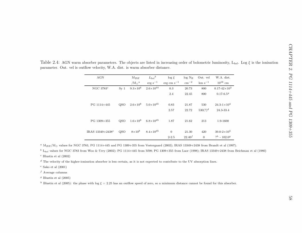
CH
AP
TE
R2.
PG
1114+445
and
PG
1309+355
58
Table 2.4: AGN warm absorber parameters. The objects are listed in increasing order of bolometric luminosity, Lbol. Log ξ is the ionisation
parameter. Out. vel is outflow velocity, W.A. dist. is warm absorber distance.
AGN MBH Lbolb log ξ log Nh Out. vel W.A. dist.
/Ma erg s−1 erg cm s−1 cm−2 km s−1 1018 cm
NGC 3783c Sy 1 9.3×10⁶ 2.6×1044 0.3 20.73 800 0.17-42×103
2.4 22.45 800 0.17-6.5g
PG 1114+445 QSO 2.6×10⁸ 5.0×1045 0.83 21.87 530 24.3-1×10⁴
2.57 22.72 530(?)d 24.3-33.4
PG 1309+355 QSO 1.6×10⁸ 6.8×1045 1.87 21.62 213 1.9-1600
IRAS 13349+2438e QSO 8×10⁸ 8.4×1045 0 21.30 420 39.0-2×10⁵
2-2.5 22.40f 0 ?h - 102.0g
a MBH/M values for NGC 3783, PG 1114+445 and PG 1309+355 from Vestergaard (2002); IRAS 13349+2438 from Brandt et al (1997).
b Lbol values for NGC 3783 from Woo & Urry (2002); PG 1114+445 from M98; PG 1309+355 from Laor (1998); IRAS 13349+2438 from Beichman et al (1980)
c Blustin et al (2002)
d The velocity of the higher-ionisation absorber is less certain, as it is not expected to contribute to the UV absorption lines.
e Sako et al (2001)
f Average columns
g Blustin et al (2005)
h Blustin et al (2005): the phase with log ξ = 2.25 has an outflow speed of zero, so a minimum distance cannot be found for this absorber.

Chapter 3
The Seyfert 1 AGN H 0557-385
H0557−385 (also known as 3A 0557-383, EXO055620-3820.2 and CTS B31.01) is
a Seyfert 1 AGN at redshift 0.034 (Fairall, McHardy & Pye 1982). The Galactic
neutral column density towards it is 4×1020cm−2 (Dickey & Lockman 1990).
In this thesis I report the first observations of this source with XMM-Newton.
H 0557-385 has also been observed with ASCA (Turner et al 1996) and BeppoSAX
(Quadrelli et al 2003). Both previous observations detected a warm absorber. In
this work I explore the details of the warm absorption in H0557-385, using both
EPIC and RGS data.
H 0557−385 was observed with XMM-Newton (Jansen et al 2001) on 3rd
April 2002 and 17th September 2002; the observation details are summarised in
Table 3.1.
The EPIC pn data were taken in large window mode, and the MOS data
in small window mode, both using the thin filter. Periods of high background,
identified in 5-10 keV lightcurves for the whole field of view outside the source
region, were excluded. The data were processed using the Science Analysis Sys-
tem (SAS) Version 6; the pn spectra were accumulated using single and double
events, corresponding to PATTERN values of 0-4, and the MOS spectra were
constructed using all valid events (PATTERN = 0-12). The count rates are be-
low the thresholds where pile-up has to be considered (12 counts s−1 for the pn
59
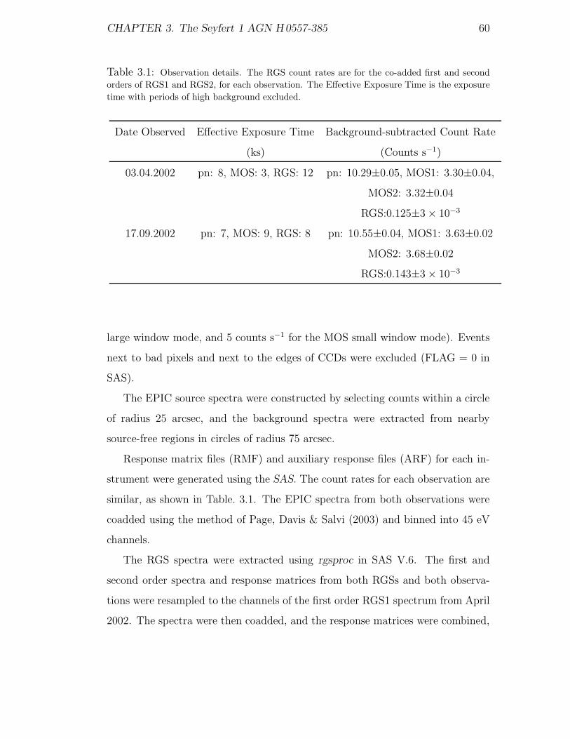
CHAPTER 3. The Seyfert 1 AGN H0557-385 60
Table 3.1: Observation details. The RGS count rates are for the co-added first and second
orders of RGS1 and RGS2, for each observation. The Effective Exposure Time is the exposure
time with periods of high background excluded.
Date Observed Effective Exposure Time Background-subtracted Count Rate
(ks) (Counts s−1)
03.04.2002 pn: 8, MOS: 3, RGS: 12 pn: 10.29±0.05, MOS1: 3.30±0.04,
MOS2: 3.32±0.04
RGS:0.125±3 × 10⁻³
17.09.2002 pn: 7, MOS: 9, RGS: 8 pn: 10.55±0.04, MOS1: 3.63±0.02
MOS2: 3.68±0.02
RGS:0.143±3 × 10⁻³
large window mode, and 5 counts s−1 for the MOS small window mode). Events
next to bad pixels and next to the edges of CCDs were excluded (FLAG = 0 in
SAS).
The EPIC source spectra were constructed by selecting counts within a circle
of radius 25 arcsec, and the background spectra were extracted from nearby
source-free regions in circles of radius 75 arcsec.
Response matrix files (RMF) and auxiliary response files (ARF) for each in-
strument were generated using the SAS. The count rates for each observation are
similar, as shown in Table. 3.1. The EPIC spectra from both observations were
coadded using the method of Page, Davis & Salvi (2003) and binned into 45 eV
channels.
The RGS spectra were extracted using rgsproc in SAS V.6. The first and
second order spectra and response matrices from both RGSs and both observa-
tions were resampled to the channels of the first order RGS1 spectrum from April
2002. The spectra were then coadded, and the response matrices were combined,

CHAPTER 3. The Seyfert 1 AGN H0557-385 61
to produce a single spectrum and a single response matrix. The spectrum was
then binned by a factor of 9 to improve signal to noise, giving a binsize of 0.1 A
at 20 A. The data were analysed using SPEX 2.00 (Kaastra et al 2002). I adopt
a cosmology with H0 = 70.0 km s−1 Mpc−1, Ωm = 0.3 and Ωλ = 0.7.
3.1 Fits to the EPIC data
The combined pn and MOS data were fitted in SPEX with a number of spectral
models: the fit parameters are listed in Table 3.2. Figs. 3.1-3.6 show the spectra
and data/model ratios for the combined pn and MOS data. All spectra are
plotted in the observed frame, unless otherwise stated.
Absorption by the Galactic column density is included in all the fits, using
the model hot, in SPEX. This is for a gas in collisional ionisation equilibrium,
set at the minimum temperature (5×10⁻⁴ keV), and it produces a very similar
spectrum to that of a pure photoelectric model (e.g. Morrison & McCammon
1983), but includes absorption lines as well as absorption edges.

CHAPTER 3. The Seyfert 1 AGN H0557-385 62
Figure 3.1: Power law fit (Model A).
Figure 3.2: Fit with one warm absorber (Model B).

CHAPTER 3. The Seyfert 1 AGN H0557-385 63
Figure 3.3: Fit with two warm absorbers (Model C).
Figure 3.4: Fit with two warm absorbers and neutral absorption (Model D).
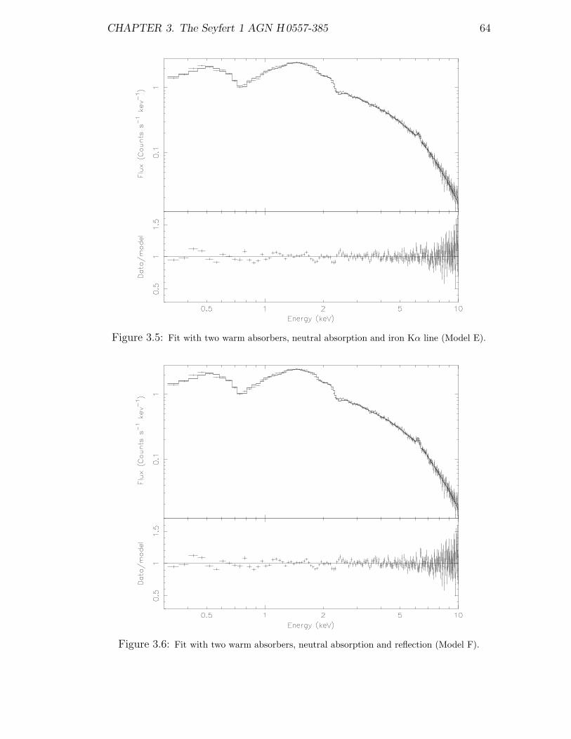
CHAPTER 3. The Seyfert 1 AGN H0557-385 64
Figure 3.5: Fit with two warm absorbers, neutral absorption and iron Kα line (Model E).
Figure 3.6: Fit with two warm absorbers, neutral absorption and reflection (Model F).

CHAPTER 3. The Seyfert 1 AGN H0557-385 65
I started by fitting a simple power law in the range 2.3-10 keV (Model A)
to avoid the regions where the low-energy absorption affects the spectrum. In
Fig. 3.1 the power law is plotted back to 0.3 keV to show the shape and extent of
the absorption. The plot is suggestive of the presence of a warm absorber, with
the deepest trough occuring at ∼ 0.7 keV; at this energy this will be a warm,
rather than a neutral absorber.
To fit the whole spectrum, a warm absorber component (xabs in SPEX) was
added to the model (Model B). The xabs component models absorption by a
cloud of photoionised gas, at a given column and ionisation parameter, where
the ionisation parameter is defined as ξ = L/nr2 in erg cm s−1. As mentioned
previously, L is the 1-1000 Rydberg ionising luminosity (erg s−1), n the gas density
(cm−3), and r the distance of the ionising source from the absorbing gas, in
cm. The turbulent velocity of the gas is set to 100 km s−1, and the elemental
abundances to solar values. Only the column and ionisation parameter were left
free in the fitting.
Including the warm absorber in the model brings it to resemble the data far
more closely, as shown in the plot for Model B. However, the χ2/dof is 946/211,
and the model is still not a good match to the data at some energies. The single
xabs component has created an absorption feature in the model which is deeper
than that in the data at ∼ 0.75 keV, but the model has insufficent absorption at
1 keV, as examination of the data/model ratio in Fig. 3.2 shows.
Another xabs component with a much higher ionisation parameter was added
(Model C): this reduces the ionisation parameter and column of the first xabs
component and provides a better fit to the data at ∼ 0.75 keV and 1 keV, as
shown in Fig. 3.3. The goodness of fit is significantly improved, but the model
still appears to require some absorption at ∼ 0.3-0.4 keV to match the data.
Therefore a component of neutral gas (again, using hot in SPEX at the minimum
temperature of 5×10⁻⁴ keV) was added at the same redshift as H 0557−385. The
column density of neutral gas, 4×1020 cm−2, provides a much better fit to the
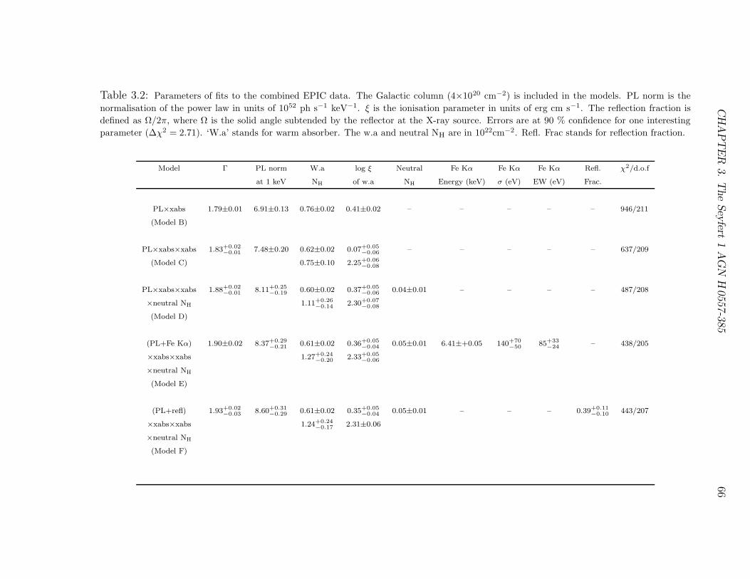
CH
AP
TE
R3.
The
Sey
fert1
AG
NH
0557-38566
Table 3.2: Parameters of fits to the combined EPIC data. The Galactic column (4×1020 cm−2) is included in the models. PL norm is the
normalisation of the power law in units of 1052 ph s−1 keV−1. ξ is the ionisation parameter in units of erg cm s−1. The reflection fraction is
defined as Ω/2π, where Ω is the solid angle subtended by the reflector at the X-ray source. Errors are at 90 % confidence for one interesting
parameter (∆χ2 = 2.71). ‘W.a’ stands for warm absorber. The w.a and neutral Nh are in 1022cm−2. Refl. Frac stands for reflection fraction.
Model Γ PL norm W.a log ξ Neutral Fe Kα Fe Kα Fe Kα Refl. χ2/d.o.f
at 1 keV Nh of w.a Nh Energy (keV) σ (eV) EW (eV) Frac.
PL×xabs 1.79±0.01 6.91±0.13 0.76±0.02 0.41±0.02 – – – – – 946/211
(Model B)
PL×xabs×xabs 1.83+0.02−0.01 7.48±0.20 0.62±0.02 0.07+0.05
−0.06 – – – – – 637/209
(Model C) 0.75±0.10 2.25+0.06−0.08
PL×xabs×xabs 1.88+0.02−0.01 8.11+0.25
−0.19 0.60±0.02 0.37+0.05−0.06 0.04±0.01 – – – – 487/208
×neutral Nh 1.11+0.26−0.14
2.30+0.07−0.08
(Model D)
(PL+Fe Kα) 1.90±0.02 8.37+0.29−0.21
0.61±0.02 0.36+0.05−0.04
0.05±0.01 6.41±+0.05 140+70
−5085+33
−24– 438/205
×xabs×xabs 1.27+0.24−0.20
2.33+0.05−0.06
×neutral Nh
(Model E)
(PL+refl) 1.93+0.02−0.03 8.60+0.31
−0.29 0.61±0.02 0.35+0.05−0.04 0.05±0.01 – – – 0.39+0.11
−0.10 443/207
×xabs×xabs 1.24+0.24−0.17 2.31±0.06
×neutral Nh
(Model F)
CHAPTER 3. The Seyfert 1 AGN H0557-385 67
data at lower energies, as shown in Fig. 3.4 (Model D). With the addition of
neutral gas, the column of the high-ξ absorber increases and the model fits the
data more closely at ∼ 0.3-0.4 keV and ∼ 0.5-1 keV.
Now the soft X-ray spectrum is fitted well, I turn to the hard X-ray spectrum.
An iron Kα line is visible at ∼ 6 keV and I first modelled it with a gaussian. This
improved the χ2 by 49 for 3 extra parameters (Model E). The energy of the line
is 6.41±0.05 keV, with a FWHM of 330+170−130 eV and equivalent width of 85+33
−24
eV. The fit is shown in Fig. 3.5. As this line may originate by fluorescence in
reflecting material, I next tried a reflection model (refl in SPEX), which includes
an iron Kα line, in combination with Model D. As the energy of the line indicates
it comes from cold material, I assume the reflecting material is cold. The best-fit
reflected fraction is 0.39+0.11−0.10. The addition of this component improves the χ2
by 44 from Model D. This is shown in Fig. 3.6, and is Model F. As the reflected
fraction is small, and the addition of this component produces a slightly worse
χ2 than Model E, I conclude that the inclusion of reflection is not justified and
that the iron Kα line alone is a sufficient addition to Model D. I then take Model
E as the best-fit to the EPIC data.
The 2-10 keV flux of model E is 4.3±0.1 × 10⁻¹¹ erg s−1 cm−2, compared to
2×10⁻¹¹ erg s−1 cm−2 at the time of the ASCA observation of Turner et al (1996)
and 4×10⁻¹¹ erg s−1 cm−2 at the time of the BeppoSax observation of Quadrelli
et al (2003). The 1-1000 Rydberg luminosity of model E is 4.3×1044 erg s−1.
3.2 Fits to the RGS data
I now investigate the soft X-ray absorption features using the RGS, which has
much higher energy resolution (E/∆E ∼ 200-800) than EPIC (E/∆E ∼ 20-50).
The EPIC best-fit, model E, was plotted on to the RGS spectra after con-
volving it with the RGS response; the result is shown in Fig. 3.7. RGS and EPIC
cross-calibration shows discrepancies of up to 15 % in the band 6 A -18 A and

CHAPTER 3. The Seyfert 1 AGN H0557-385 68
up to 10 % in ∼ 18 A -36 A (Fig 11 of Kirsch et al 2004). The spectral shape
and flux of H 0557−385 are generally well reproduced, but this model does not
match the RGS data completely. It overestimates the data over ∼ 8-15 A and ∼23-33 A and is too absorbed at ∼ 18-19 A . In order to obtain a better fit to the
RGS data, the continuum from EPIC model E was kept fixed, and the columns
and ionisation parameters of the absorbers in the model were left to vary. I con-
sider only the 8-30 A spectrum, where RGS calibration and statistical quality
of the data are best. The turbulent velocity of the gas was again set to 100 km
s−1. The absorbers were set at the recession velocity of the AGN. The resultant
best-fit proved to be in much better agreement with the RGS data, and is shown
in Fig. 3.8, along with the data/model ratio. The main ions from each absorbing
phase are indicated. The parameters from the EPIC model E and RGS fits are
compared in Table. 3.3.
As the RGS has better energy resolution than EPIC, the best-fit model will
be closer to the real characteristics of the source. As shown in Table. 3.3, the
parameters of the warm absorbers required by the RGS data are different to those
from the EPIC data. With respect to the EPIC data, for the RGS the column of
the low-ξ phase is lower whereas the column of the high-ξ phase has not changed.
The log ξ values of the low-ξ phase are consistent, but the log ξ of the high-ξ
phase is smaller than that derived from the EPIC data. A much larger column
of neutral gas is also required.
Compared to Fig. 3.7, the model in Fig. 3.8 is now a much better fit to the
data at 8-15 A and from 17 A onwards. The χ2/dof of the model shown in
Fig. 3.7 is 413/236, whereas the χ2/dof of the RGS best-fit model (Fig. 3.8) is
246/231. The discrepancy between the data and the model at ∼ 18-19 A in
Fig. 3.7 has disappeared.
Fig. 3.9 shows the models corresponding to the high-ξ and low-ξ phases. The
deep and broad absorption feature at ∼ 16-18 A, clearly visible in the RGS
spectrum, is the signature of an unresolved transition array (UTA) of M-shell
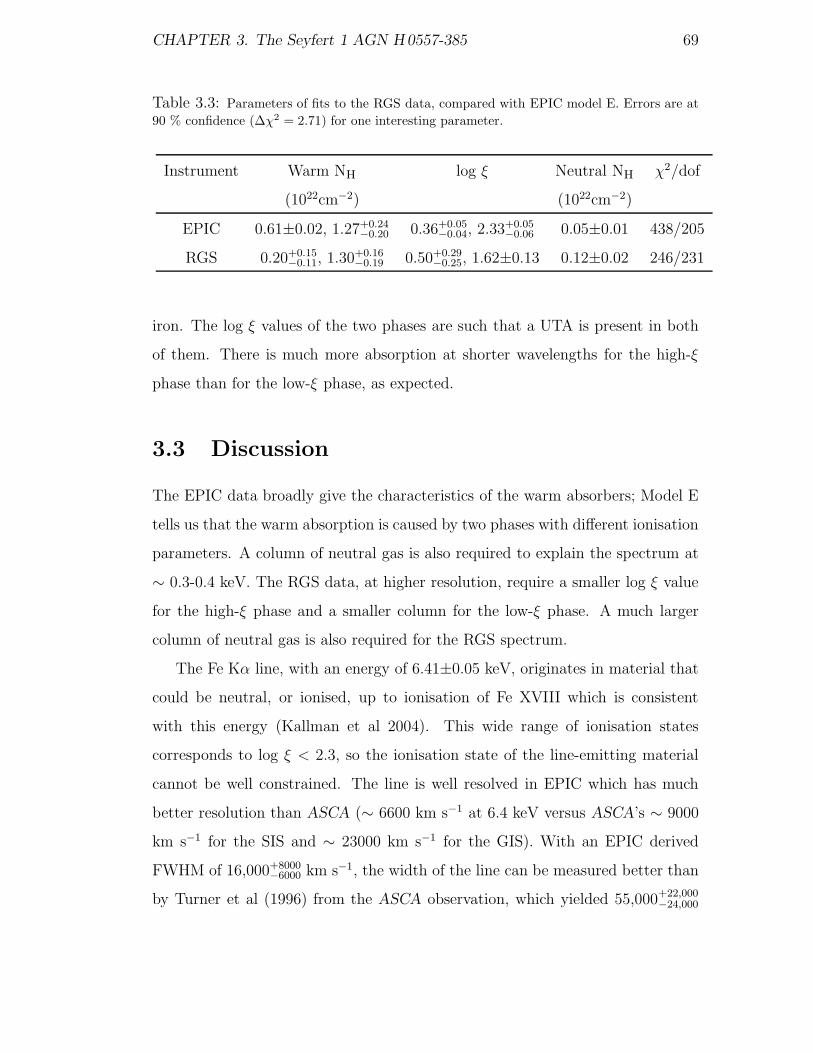
CHAPTER 3. The Seyfert 1 AGN H0557-385 69
Table 3.3: Parameters of fits to the RGS data, compared with EPIC model E. Errors are at
90 % confidence (∆χ2 = 2.71) for one interesting parameter.
Instrument Warm Nh log ξ Neutral Nh χ2/dof
(1022cm−2) (1022cm−2)
EPIC 0.61±0.02, 1.27+0.24−0.20 0.36+0.05
−0.04, 2.33+0.05−0.06 0.05±0.01 438/205
RGS 0.20+0.15−0.11, 1.30+0.16
−0.19 0.50+0.29−0.25, 1.62±0.13 0.12±0.02 246/231
iron. The log ξ values of the two phases are such that a UTA is present in both
of them. There is much more absorption at shorter wavelengths for the high-ξ
phase than for the low-ξ phase, as expected.
3.3 Discussion
The EPIC data broadly give the characteristics of the warm absorbers; Model E
tells us that the warm absorption is caused by two phases with different ionisation
parameters. A column of neutral gas is also required to explain the spectrum at
∼ 0.3-0.4 keV. The RGS data, at higher resolution, require a smaller log ξ value
for the high-ξ phase and a smaller column for the low-ξ phase. A much larger
column of neutral gas is also required for the RGS spectrum.
The Fe Kα line, with an energy of 6.41±0.05 keV, originates in material that
could be neutral, or ionised, up to ionisation of Fe XVIII which is consistent
with this energy (Kallman et al 2004). This wide range of ionisation states
corresponds to log ξ < 2.3, so the ionisation state of the line-emitting material
cannot be well constrained. The line is well resolved in EPIC which has much
better resolution than ASCA (∼ 6600 km s−1 at 6.4 keV versus ASCA’s ∼ 9000
km s−1 for the SIS and ∼ 23000 km s−1 for the GIS). With an EPIC derived
FWHM of 16,000+8000−6000 km s−1, the width of the line can be measured better than
by Turner et al (1996) from the ASCA observation, which yielded 55,000+22,000−24,000

CHAPTER 3. The Seyfert 1 AGN H0557-385 70
Figure 3.7: The RGS spectrum, plotted in the observed frame with the best-fit EPIC model
E superimposed. The data/model ratio is also shown.

CH
AP
TE
R3.
The
Sey
fert1
AG
NH
0557-38571
−−−− UTA of M−Shell Fe
α
α
α
−−−− O VIII Ly (hot phase)
−−−− N VII Ly (both phases)
−−−− N VI He (both phases)
α −−−− Ne X Ly (hot phase)
α −−−− Ne IX He (hot phase)
α −−−− O VII He (both phases)
−−
−−
−−
−− (both phases)
−−−− O I (neutral absorber) −−−− O I edge (neutral absorber)
Figu
re3.8:
The
RG
Ssp
ectrum
,plo
ttedin
the
observ
edfra
me
with
the
best-fi
tR
GS
model.
Som
eofth
em
ain
abso
rbin
gio
ns
that
belo
ng
toea
chphase
are
labelled
.T
he
data
/m
odel
ratio
isalso
show
n.
−−−−−−−−−−−−−−− O VII He (both phases)α
α
−−−−−−−−−−−−−−−−−− UTA of M−Shell Fe −−
−−
− −
−
−−−−−−−−−−−−−−− O VIII Ly (hot phase)
−−−−−−−−−−−−−−− O I (neutral absorber)
−−−−−−−−−−−−−−− Ne X Ly (hot phase)α
α−−−−−−−−−−−−−−−− Ne IX He (hot phase)
(both phases)
−−−−−−−−−−−−−−−−− N VII Ly (both phases)α
−−−−−−−− N VI He (both phases)α
−−−−−−−−−−−−−−− O I edge (neutral absorber)
Figu
re3.9:
The
RG
Sbest-fi
tm
odel,
plo
ttedin
the
observ
edfra
me,
for
the
two
abso
rber
phases.
Bla
ck:
hig
h-ξ
phase.
Grey
:low
-ξphase.
The
top
dotted
curv
e,sh
own
inbla
ck,is
the
unabso
rbed
contin
uum
;th
elow
ercu
rve,
also
inbla
ck,in
cludes
the
neu
tralgas.
The
Gala
ctic
colu
mn
isnot
inclu
ded
inany
ofth
em
odels
inth
isplo
t.
.
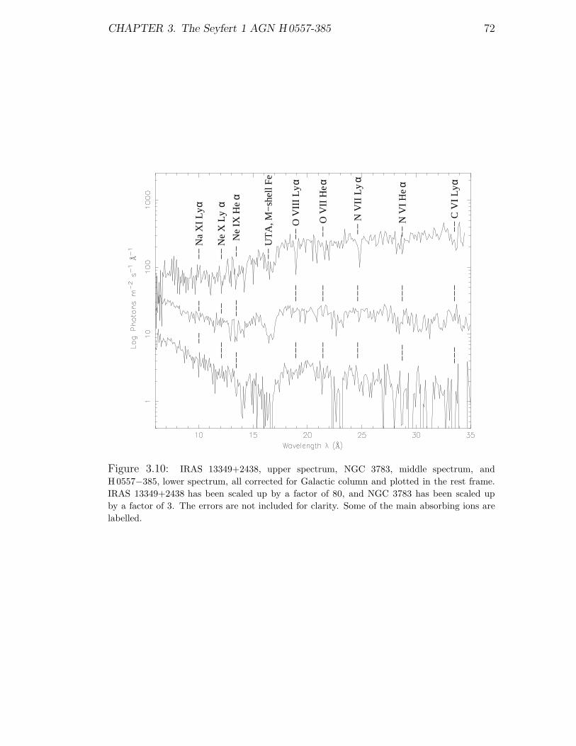
CHAPTER 3. The Seyfert 1 AGN H0557-385 72
−−
N V
I H
e α α
−−
−
−−
−
−−
−
−−
−
−
−−
−
−−
−
−−
−
−−
−
−−
−
−−
−
−−
−−
−
−−
Ne
X L
y
−−
Ne
IX H
e
α αα
−−
O V
III
Ly
−−
O V
II H
e
−−
N V
II L
y
−−
C V
I L
y α α α
−−
UT
A, M
−sh
ell F
e
−−
Na
XI
Ly
−−
−
−−
−
−−
−
Figure 3.10: IRAS 13349+2438, upper spectrum, NGC 3783, middle spectrum, and
H 0557−385, lower spectrum, all corrected for Galactic column and plotted in the rest frame.
IRAS 13349+2438 has been scaled up by a factor of 80, and NGC 3783 has been scaled up
by a factor of 3. The errors are not included for clarity. Some of the main absorbing ions are
labelled.

CHAPTER 3. The Seyfert 1 AGN H0557-385 73
km s−1. I find the equivalent width of the line to be 85+33−24 eV, compared with ∼
300 eV found by Turner et al (1996).
From optical spectroscopy, Rodrıguez-Ardila et al (2000) distinguish 3 Hα
components in H0557−385. The FWHM of the narrowest component is 1035
km s−1, that of the intermediate component is 2772 km s−1 and for the broadest
component it is 11,000 km s−1. The last value suggests that the region that
produces the broadest Hα component could also be the location of the Fe Kα
line emitting gas.
To start to build up a picture of the AGN as a whole, I use the relation in
Krolik & Kriss (2001) to estimate the approximate distance to the inner edge of
the torus, Rtorus, in cm, from the continuum source with ionising luminosity L,
in erg s−1:
Rtorus, cm ∼ 3 × 10⁻⁴√
L (3.1)
This is equivalent to Equation. 2.10 expressed in cgs units. Using the 1-1000
Rydberg luminosity from the EPIC best-fit model, i.e. L = 4.3×1044 erg s−1, I
obtain 6.2×1018 cm (∼ 2 pc) for the inner radius of the torus.
To place a distance on the Fe Kα line formation region from the black hole, I
use a black hole mass of 3×10⁷ M. This value is intermediate to the Schwarzchild
and Kerr black hole masses measured for H 0557−385 by Rokaki & Boisson (1999),
who assume that Hβ emission lines come from the disk. I use the FWHM of 16,000
km s−1 of the Fe Kα line as v in the equation:
v =
√
GM
R(3.2)
to obtain the distance, R, of the line formation region from the black hole, assum-
ing the line emitting gas moves in a Keplarian orbit: I obtain a distance of 2×10¹⁵
cm. The Schwarzchild radius for the black hole, 2GM/c2, will be 9×1012 cm. If
I take the inner edge of the accretion disk to be 6GM/c2, then for H 0557−385
this is 3×1013 cm. For the Hα line I find distances of 4×1017 cm, 5×1016 cm, and
3×1015 cm for the narrowest, intermediate and broadest components respectively.

CHAPTER 3. The Seyfert 1 AGN H0557-385 74
The distance of the broadest Hα line is very close to that of the Fe Kα line, which
suggests that these lines both come from the same place.
3.3.1 Where did the warm absorbers originate?
I now try to determine the distances of the warm absorbers from the continuum
source, and thus find some clue as to their origins.
I assume the warm absorbers to be a continous, constant velocity wind. I
use Rl as the launching radius of the wind; for such a wind, Nh = nlRlf and
ξ = L/nlR2l . L is the 1-1000 Rydberg luminosity (4.3×1044 erg s−1 from the
EPIC best-fit model), nl is the density at Rl and f is the volume filling factor of
the gas. Substituting to eliminate nl, I obtain
L =ξNhRl
f(3.3)
Taking the upper limit of the volume filling factor, f = 1, and including the 90
per cent confidence limits on the other parameters, I obtain upper limits of Rl ≤1×1021 cm to the higher-ξ absorber, and Rl ≤ 2×1023 cm to the lower-ξ absorber.
Unfortunately, the locations of the warm absorbers cannot be constrained any
better from the data available.
3.3.2 Comparison with other AGN
NGC 3783 and IRAS 13349+2438 are AGN with warm absorbers that display
significant UTAs, similar to H0557−385. A comparison of their RGS spectra,
corrected for redshift and Galactic column, is shown in Fig. 3.10, and the param-
eters of the warm absorbers observed in these AGN are listed in Table 3.4.
The warm absorbers of these three AGN exist in multiple phases and are
parameterised as two phases from the RGS observations. More recently, Netzer
et al (2003) conducted a more detailed study into NGC 3783 using Chandra
data, finding that the warm absorption exists in three phases, that correspond

CHAPTER 3. The Seyfert 1 AGN H0557-385 75
Table 3.4: Comparison of warm absorber parameters for the type 1 AGN NGC 3783,
IRAS 13349+243 and H 0557−385.
AGN Nh log ξ
(1022cm−2)
NGC 3783a 0.054+1×10⁻³
−5×10⁻³, 2.8+0.0−0.3 0.3, 2.4
IRAS 13349+2438b 0.2±0.1, 2.5±1.5 0, 2.25
H0557−385 0.20+0.15−0.11, 1.30+0.16
−0.19 0.50+0.29−0.25, 1.62±0.13
a Blustin et al (2002) b Sako et al (2001)
to log ξ values of 1.1, 2.3 and 2.9; however the RGS derived parameters of these
AGN are directly compared for consistency. From the RGS observation, the
warm absorbers of NGC 3783 have a combined log Nh value of 22.5, and those
of IRAS 13349+2438 have a combined log Nh of 22.4. H 0557−385 is more
heavily absorbed than the other two; it has a combined log Nh of 22.2, but also
has an intrinsic neutral gas component, which absorbs it particularly at longer
wavelengths, although this component has a much smaller column (log Nh of
21.1).
In H0557−385 the ionisation parameters of the two phases are such that the
UTA is produced in both, but in NGC 3783 and IRAS 13349+2438 the UTA only
comes from the lower-ξ phase. The column of the lower-ξ phase in NGC 3783 is
much smaller than the lower-ξ phase columns in the other two AGN; however,
in the spectral fitting of Blustin et al (2002), it was found that iron needs to be
overabundant by a factor of ∼ 10 with respect to C, N and O in order to account
for the depth of the UTA, so the column for the low-ξ phase should effectively be
considered as ten times higher than that listed in Table 3.4.

CHAPTER 3. The Seyfert 1 AGN H0557-385 76
3.3.3 Where is the neutral gas component?
I find that the RGS data of H 0557−385 require absorption from neutral gas
local to the galaxy, of density 1.20×1021cm−2. But where is this gas in the AGN
structure? Fairall, McHardy & Pye (1982) and Rafanelli (1985) found the optical
emission lines of H 0557−385 heavily reddened. Therefore if it is assumed that
dust is mixed with the neutral absorber, then both must lie outside the broad
line region. There are therefore three main possibilities for the location of the
neutral gas: the AGN itself, the disk of the host galaxy, or somewhere in the host
galaxy but outside the disk.
Scenario 1:
The first possibility is gas within the AGN itself. If the warm absorber is a wind
formed by evaporation from the dusty torus, then the neutral gas could be from
the torus. Ogle (2003) suggests that the torus has a role in defining the shape
of the ionisation cone. As the continuum source must be viewed through the
ionisation cone to see a warm absorber, we cannot be looking directly through
the side of the torus. However, it could be that we are seeing cold absorption
through a small cross-section of the torus if our line of sight grazes the edge.
Scenario 2:
The second possibility is the disk of the host galaxy. H 0557−385 is classified
as S0a in the Nasa Extragalactic Database, between a spiral and a lenticular
galaxy. It is observed at an inclination angle i = 75 from the normal (Crenshaw
& Kraemer 2001). If the host galaxy of H 0557−385 has similar column density
values to other Sa galaxies, then the neutral absorption observed could originate
in the host galaxy of the AGN. The average neutral hydrogen column density for
an Sa galaxy viewed face-on, Nh⊥, is 1.4×1021 cm−2 (Broeils & Woerden 1994).
Using the relation Nh = Nh⊥/cos i, I obtain an expected value of 5.3×1021 cm−2
for Nh. This is larger than the neutral column observed in H0557−385, so it is

CHAPTER 3. The Seyfert 1 AGN H0557-385 77
plausible the neutral gas in H0557−385 could originate in the disk of the host
galaxy.
Scenario 3:
The third possibility for the origin of this neutral gas is outside the AGN and
above the disk of the galaxy, but within the structure of the galaxy. It could be
in the form of a dust lane. From HST images, Malkan, Gorjian & Tam (1998)
find that there are dust lanes at distances of hundreds of parsecs in Seyfert 1 and
2 AGN. These dust lanes have little or no connection with the central engine and
could have column densities up to ∼ 1023 cm−2 (Matt et al 2000). Such a dust
lane could therefore plausibly supply a column of ∼ 1021 cm−2.
Given these three scenarios, I consider that all possibilities are plausible. Since
some of the values of Rl (the launching radius of the wind) for different AGN in
Table 4.1 are on similar scales to those of Scenario 3, it may be that the cold
gas can exist on similar scales to the warm absorbers; this is plausible given the
small filling factors of the warm absorbers.
3.4 Conclusion
From XMM-Newton RGS observations of the Seyfert 1 AGN H0557−385 I find
that warm absorption is present in two phases, a low-ξ phase with log ξ of 0.50
and a column of ∼ 1021 cm−2 and a high-ξ phase with log ionisation parameter ξ
of 1.62 and a column of ∼ 1022 cm−2. An unresolved transition array of (M-shell)
iron is detected in both phases of the absorber.
I infer a picture of the different scales of these components. The locations of
the warm absorbers are not well constrained (≤ 1021-1023 cm from the central
continuum source), compared to the molecular torus distance of ∼ 1018 cm from
the source of the ionising luminosity. The Fe Kα line and a broad Hα line are
both likely to originate at ∼ 1015 cm from the black hole.

CHAPTER 3. The Seyfert 1 AGN H0557-385 78
From a comparison with NGC 3783 and IRAS 13349+2438, AGN with warm
absorbers that also have significant UTAs similar to H0557−385, I find that
H0557−385 is more heavily absorbed than the other two.
A column of neutral gas is observed, that could originate from the AGN torus,
the host galaxy disk, or a lane or cloud of gas above the disk.

Chapter 4
Discussion
In this thesis I have examined the X-ray warm absorber outflows from two quasars,
PG 1114+445 and PG 1309+355, and a Seyfert 1 AGN, H0557−385. I will now
use these results to improve our understanding of the nature and origin of warm
absorbers in general.
Fig. 4.1 and Fig. 4.2 show plots of log Lbol versus log ξ and versus log total
absorbing column for the sample of 23 AGN studied by Blustin et al (2005; here-
after B05), to which I have added (from this thesis) PG 1114+445, PG 1309+355,
and H0557−385, and also the quasar PDS 456 (Reeves et al 2003).
From these graphs, we see that PG 1114+445 and PG 1309+355 sit at the
lower luminosity end of the quasars, and H0557−385 lies at the high luminosity
end of the Seyferts. The columns and ionisation parameters of all three are within
the range currently observed for AGN warm absorbers. I have already pointed
out in Chapter 2 that the ionisation parameters of warm absorbers in at least
some quasars are similar to those in Seyfert galaxies.
4.0.1 Connection with X-ray and UV absorbers
A UV absorber was known to exist in PG 1114+445 (M98), and from my detailed
study of X-ray warm absorption in this quasar, I find that the UV absorber is
79

CHAPTER 4. Discussion 80
Figure 4.1: Log Lbol versus log ξ; updated from Blustin et al (2005). Quasars are triangles
and Seyferts are circles. PG 1114+445 and PG 1309+355 are filled triangles, and H 0557−385
is a filled circle.
Figure 4.2: Log Lbol versus log NHtotal; updated from Blustin et al (2005). Quasars are
triangles and Seyferts are circles. PG 1114+445 and PG 1309+355 are filled triangles, and
H 0557−385 is a filled circle.

CHAPTER 4. Discussion 81
associated with the lower-ξ X-ray absorber. Warm absorption had not been
observed in PG 1309+355, before the XMM-Newton detection reported in this
thesis. It is likely the X-ray absorber is associated with the UV absorber also in
this source.
4.0.2 Where can we place the warm absorbers?
A crucial part of the study of warm absorbers is endeavouring to find their loca-
tions in the structure of AGNs. Whilst I am not able to find their exact locations,
I can put some useful limits on them.
For PG 1114+445 and PG 1309+355, I estimate the distance range of the
warm absorbers, as well as the distances of the BLR and the torus. For both
AGN, the absorbers lie further out from the continuum source than the BLR,
and also further out than the inner edge of the torus. This suggests that the
warm absorbers in both AGN originate as a torus wind.
For H0557−385 I can only estimate the upper distances to the absorbers;
these distances include the inner edge of the torus, so a torus wind is a possibility
for the origin of the absorbers in this AGN too.
4.0.3 A torus origin for warm absorbers?
Below I describe a method to determine the filling factors of warm absorbers, and
I compare my findings for a sample of AGN. I then discuss the implications they
have on the suggested origin of warm absorbers in torus winds.
From the relation for the ionisation parameter, ξ = L/nr2, I infer that for
constant density and ξ, r scales with L1/2. Equation 3.1 expresses the same scaling
relation, for the inner edge of the torus. Here, r is the distance of the ionising
source from the absorbing gas. From this I can infer that if warm absorbers
originate at the inner edge of the torus then they should possess similar values
of the product of ionisation parameter and density, independent of their ionising

CHAPTER 4. Discussion 82
luminosities.
I re-write Equation 3.1 as Rtorus ∼ K√
L with K = 3×10⁻⁴. Then re-arranging
Equation 3.3 (L = ξNHRl
f), equating Rl to Rtorus, and substituting for Rtorus, I
obtain
L1/2 ' ξNhK
f(4.1)
Taking logs of both sides then working through the algebra, I obtain
log L ' 2 log ξNh − 2 logf
K(4.2)
This implies a linear relationship between log L and log ξNh with a gradient
of 2 and an intercept of −2 log fK
. A list of log Nh, log ξ and log L values for
warm absorbers observed in 14 AGN is given in Tables 2 and 4 of B05. These
authors assume a constant velocity wind in considering the energetics of warm
absorbers. In Fig. 4.3, log L is plotted versus log ξNh for the AGN in B05 along
with the parameters derived for H 0557−385 from the RGS data. We can now
use Equation 4.2 to calculate the filling factor f for all the AGN in Fig. 4.3. The
filling factors for all absorber phases are listed in Table 4.1.
The absorber of PG 0844+349 and one of the absorbers in PG 1211+143
would have filling factors larger than 1 if they originated at the inner edge of the
torus, so they cannot originate as torus winds. Pounds et al (2003a, 2003b) and
B05 argue that the absorbers in these objects originate as accretion disk winds;
from Table 4.1 these must originate closer in than the torus, so the results are
consistent with an accretion disk wind.
In Table 4.1 there are 5 absorbers for which I compute very low filling factors
(f < 10−4). These absorbers have the smallest values of log ξ in the sample,
ranging from 0 to 0.68 (except for the absorber with log ξ = 2 in Ark 564). The
AGN in question are H0557−385, MR 2251-178, IRAS 13349+2438, NGC 4593,
NGC 5548 and Ark 564.

CHAPTER 4. Discussion 83
Figure 4.3: Log values of ionising luminosity, versus the log of the product of ionisation
parameter and column density, for 14 AGN. H 0557−385 is shown as starred points, along
with errors. Data for all other AGN are from B05. The warm absorbers in PG 0844+349 and
PG 1211+143, believed to be accretion disk winds, are shown as triangles. Some different filling
factors are represented as the diagonal lines and labelled at the bottom. PG 1114+445 and
PG 1309+355 are not included as this Figure was limited to results from high-resolution data.

CHAPTER 4. Discussion 84
In Fig. 4.4 the filling factors for the AGN as listed in Table 4.1 are plotted,
versus those found by BO5. My method for calculating filling factors compared
to that of B05 has the advantage of requiring only log Nh, log ξ and log L values
for warm absorbers, and no dynamical information. In contrast, the method of
B05 uses the outflow velocities of the warm absorbers, and involves calculating
the momentum absorbed and scattered by the warm absorber.
Unsurprisingly, Equation 4.2 assigns much larger filling factors to the accretion
disk wind absorbers than B05. For the remaining objects, the absorbers with log
ξ > 0.7 are located in a different part of Fig. 4.4 to the 5 lower-ξ absorbers,
which are found on the left-hand side of the plot. The absorbers with log ξ > 0.7
have -4 < log f < 0 in both methods. Their mean log f from B05 is -1.8±0.2
with a standard deviation of 0.7, and their mean log f from this work is -2.1±0.2
with a standard deviation of 0.8 where the errors are 1 σ. Therefore the two
methods yield consistent values for 〈log f〉. It is worth comparing the standard
devations of these results with the uncertainties inherent in the two methods.
For my method I estimate the overall uncertainty on f to be approximately 0.5
dex (a sum in quadrature of 0.15 dex from L, 0.2 dex from ξ, 0.3 dex from Nh
and 0.3 dex from K, the latter from the uncertainty in the distance of the inner
edge of the torus). For the method of B05, I estimate an uncertainty on f of
approximately 0.6 dex (a sum in quadrature of 0.3 dex from L, 0.2 dex from ξ
and 0.5 dex from the absorbed and scattered momentum). Hence, the standard
deviations on f derived from the two methods are comparable with the errors
estimated for the two methods. For the absorbers with log ξ < 0.7, the mean log
f from my method is -5.1±0.1 and that of B05 is -2.6±0.3.
If the assumption that the absorbers originate at the inner edge of the torus
is relaxed, the values of Rl that would bring the two methods into agreement can
be determined, by substituting the filling factors of B05 into Equation 3.3. These
values of Rl are given in column 8 of Table 4.1. Taking the standard deviations
on f found from the high-ξ group of absorbers as the uncertainties inherent in

CHAPTER 4. Discussion 85
Figure 4.4: The filling factors derived from B05, which are translated from percentages into
a fractional scale, plotted versus the filling factors from this work. The warm absorbers in
PG 0844+349 and PG 1211+143, believed to be accretion disk winds, are shown as triangles.
A line indicating equivalence between our results and those of B05 is shown.
the two methods, and summing them in quadrature, I obtain an uncertainty of ∼1 dex. This explains why some of the values of Rl determined are very large (the
low-ξ absorbers in MR 2251-178 and Ark 564 are estimated to be greater than
3 Kpc distant from the nucleus). The mean of log Rl for the low-ξ absorbers is
2.63, so a typical distance for these absorbers is ∼ 400 pc, which is similar to the
scale of the narrow-line region (Osterbrock 1993, Capetti et al 1999). At a similar
distance from the continuum source, a photoionised cloud is seen in emission in
X-ray observations of the prototypical Seyfert 2 galaxy NGC 1068 (Brinkman
et al 2002, Ogle et al 2003). The low-ξ absorbers could be equivalent to this
photoionised cloud in NGC 1068, but seen in absorption rather than in emission.
It is unclear, though, whether such absorbers originate from the torus or from
other, more distant, material.
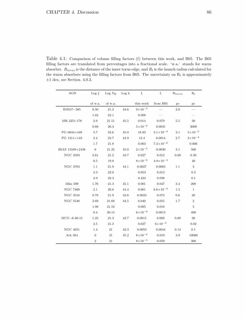
CHAPTER 4. Discussion 86
Table 4.1: Comparison of volume filling factors (f) between this work, and B05. The B05
filling factors are translated from percentages into a fractional scale. ‘w.a.’ stands for warm
absorber. Rtorus is the distance of the inner torus edge, and Rl is the launch radius calculated for
the warm absorbers using the filling factors from B05. The uncertainty on Rl is approximately
±1 dex, see Section. 4.0.3.
AGN Log ξ Log Nh Log L f, f, Rtorus Rl
of w.a. of w.a. this work from B05 pc pc
H0557−385 0.50 21.3 44.6 9×10⁻⁵ — 2.0 —
1.62 22.1 0.008 — —
MR 2251-178 2.9 21.51 45.5 0.014 0.079 5.5 30
0.68 20.3 5×10⁻⁶ 0.0031 3000
PG 0844+349 3.7 23.6 45.0 18.93 3.1×10⁻⁴ 3.1 5×10⁻⁵
PG 1211+143 3.4 23.7 44.9 13.4 0.0014 2.7 3×10⁻⁴
1.7 21.8 0.003 7.2×10⁻⁶ 0.006
IRAS 13349+2438 0 21.25 45.0 2×10⁻⁵ 0.0030 3.1 500
NGC 4593 2.61 21.2 43.7 0.027 0.012 0.69 0.30
0.5 19.8 8×10⁻⁶ 4.9×10⁻⁴ 40
NGC 3783 1.1 21.9 44.1 0.0027 0.0063 1.1 3
2.3 22.0 0.053 0.013 0.3
2.9 22.3 0.424 0.038 0.1
Mkn 509 1.76 21.3 45.1 0.001 0.047 3.4 200
NGC 7469 2.1 20.6 44.4 0.001 8.6×10⁻⁴ 1.5 1
NGC 3516 0.78 21.9 43.6 0.0023 0.072 0.6 20
NGC 5548 2.69 21.68 44.5 0.040 0.055 1.7 2
1.98 21.52 0.005 0.016 5
0.4 20.15 6×10⁻⁶ 0.0015 400
MCG -6-30-15 1.25 21.3 43.7 0.0015 0.069 0.69 30
2.5 21.3 0.027 6×10⁻⁴ 0.02
NGC 4051 1.4 21 42.3 0.0053 0.0044 0.14 0.1
Ark 564 0 21 45.2 8×10⁻⁶ 0.019 3.9 10000
2 21 8×10⁻⁴ 0.059 300
Chapter 5
Conclusions
For this thesis I have analysed XMM-Newton EPIC data of two quasars, PG 1114+445
and PG 1309+355, and EPIC and RGS data for a Seyfert 1 AGN, H0557−385.
Compared with a sample of 23 AGN with warm absorbers studied by Blustin
et al (2005), PG 1114+445 and PG 1309+355 sit at the lower luminosity end of
the quasars, and H0557−385 lies at the high luminosity end of the Seyferts.
In all three AGN I have found evidence for warm absorbers and I have studied
them in detail.
The absorption in PG 1114+445 is in two phases, a ‘hot’ phase with a log
ionisation parameter ξ of 2.57 (where ξ is in units of ergs cm s−1) and a col-
umn of 5.3×1022 cm−2, and a ‘cooler’ phase with log ξ of 0.83 and a column of
7.4×1021 cm−2. An unresolved transition array (UTA) of M-shell iron is observed
in the cooler phase. The absorption in this quasar is similar to that observed in
the Seyfert 1 NGC 3783. I have made the first detection of warm absorption in
PG 1309+355: it consists of a single phase, with log ξ of 1.87. The kinetic lumi-
nosities of these outflowing absorbers represent insignificant fractions (< 10−3) of
the energy budgets of the AGN.
For both PG 1114+445 and PG 1309+355, the absorbing gas lies at distances
of 1019 - 1022 cm from the continuum radiation source, which suggests that it
could originate in a wind emanating from a molecular torus.
87

CHAPTER 5. Conclusions 88
The warm absorption in H0557−385 can be characterised by two phases: a
phase with log ionisation parameter ξ of 0.50 and a column of 0.2×1021 cm−2,
and a phase with log ξ of 1.62 and a column of 1.3×1022 cm−2. An unresolved
transition array of (M-shell) iron is detected in both phases of the absorber. For
H0557−385 I can only estimate upper limits to the distances to the absorbers, but
they include the inner edge of the torus, so a torus wind is a possibility for the ori-
gin of the absorbers. From a comparison with NGC 3783 and IRAS 13349+2438,
AGN with warm absorbers that also have significant UTAs similar to H0557−385,
I find that H0557−385 is more heavily absorbed than the other two. A column
of neutral gas is observed, that could originate from the AGN torus, the host
galaxy disk, or a lane or cloud of gas above the disk.
UV absorption was already known to exist in PG 1114+445, and I have found
good reasons to believe that the UV absorber is associated with the lower-ξ
absorber. It is likely that the X-ray absorber in PG 1309+355 is associated with
the UV absorber in this source too.
Finally, I have established a new method of determining the volume filling
factors in warm absorbers, assuming that the ionised absorbers originate as an
outflow from the torus. I derive the volume filling factors for the Blustin et al
(2005) sample of AGN and compare them with those published, finding reason-
able agreement, although my values are generally smaller (≤ 1%) except for two
quasars, thought to possess accretion disk winds. A group of five absorbers have
filling factors derived in this work that are much smaller than those found by
Blustin et al (2005). These absorbers all have log ξ < 0.7, and putting together
my method with that used by Blustin et al (2005), I obtain distances for these
absorbers that imply they lie out in the narrow-line region, typically hundreds of
parsecs from the continuum source.

Bibliography
Antonucci R., & Miller J.S., 1985, Astrophys. J., 297, 621
Antonucci R., 1993, Ann. Rev. Astron. Astrophys., 31, 473
Barvainis R., 1987, Astrophys. J., 320, 537
Bechtold J., Dobrzycki A., Wilden B., Astrophys. J. Suppl., 2002, 140, 143
(BO2)
Behar E., Sako M., Kahn S.M., 2001, Astrophys. J., 563, 497
Beichman C.A., Soifer B.T., Helou G., Chester T.J., Neugebauer G., Gillett F.C.,
Low F.J., 1986, Astrophys. J., 308, L1
Blustin A.J., Branduardi-Raymont G., Behar E., Kaastra J.S., Kahn S.M., Page
M.J., Sako M., Steenbrugge K.C., 2002, Astr. & Astrophys., 392, 453
Blustin A.J., Branduardi-Raymont G., Behar E., Kaastra J.S., Kriss G.A., Page
M.J., Kahn S.M., Sako, M., et al, 2003, Astr. & Astrophys., 403, 481
Blustin A.J., Page M.J., Fuerst S.V., Branduardi-Raymont G., Ashton C.E.,
2005, Astr. & Astrophys., 431, 111 (B05)
Brandt W.N., Mathur S., Reynolds C.S., Elvis M., 1997, Mon. Not. R. astr. Soc.,
292, 407
Brinkman A.C., Kaastra J.S., van der Meer R. L. J., Kinkhabwala A., Behar E.,
Kahn S.M., Paerels F.B.S., Sako M., 2002, Astr. & Astrophys., 396, 761
89

REFERENCES 90
Brocksopp C., Starling R.L.C., Schady P., Mason K.O., Romero-Colmenero E.,
Puchnarewicz E.M., in press astro-ph/0510776
Broeils A.H., van Woerden H., 1994, Astr &. Astrophys. Suppl., 107, 129
Capetti A., Axon D.J., Macchetto F.D., Marconi A., Winge C., Mem. Soc.
Astron. Ital, 1999, 70, 41
Castor J.I.,, Abbott D.C., & Klein R.I., 1975, Astrophys. J., 195, 157
Crenshaw D.M., Kraemer S.B., Boggess A., Maran S.P., Mushotzky R.F., Wu,
C., 1999, Astrophys. J., 516, 750
Crenshaw D.M., Kraemer S.B., Hutchings J.B., Bradley L.D.II., Gull T.R., Kaiser
M.E., Nelson C.H., Ruiz J.R., Weistrop D., 2000, Astr. J., 120, 1731
Crenshaw D.M., Kraemer S.B., 2001, Astrophys. J., 562, L29
den Herder J.W., Brinkman A.C., Kahn S.M., Branduardi-Raymont G., Thomsen
K., Aarts H., Audard M., Bixler J.V., et al, 2001, Astr. & Astrophys., 365,
L7
Dickey J.M., Lockman F.J., 1990, Ann. Rev. Astron. Astrophys, 28, 215
Elvis M., Wilkes B.J., McDowell J.C., Green R.F., Bechtold J., Willner S.P., Oey
M.S., Polomski E., et al, 1994, Astrophys. J. Suppl., , 95, 1
Elvis M., 2000, Astrophys. J., 545, 63
Elvis M., 2004, AGN Physics with the Sloan Digital Sky Survey, ASP Conference
Series, Volume 311. San Francisco: Astronomical Society of the Pacific, 2004,
p.109
Fabian A.C., Iwasawa K., Reynolds C.S., Young A.J., 2000, PASP, 112, 1145
Fairall A.P., McHardy I.M., & Pye J.P., 1982, Mon. Not. R. astr. Soc., 198, 13P
Fanaroff B.L., & Riley J.M., 1974, MNRAS, 167, 31P
Fath E.A., 1909, Lick Observatory Bulletin 5, p.71, 1909
REFERENCES 91
George I.M., Nandra K., Laor A., Turner, T.J., Fiore F., Netzer H., Mushotzky
R.F., 1997, Astrophys. J., 491, 508
Halpern J.P., 1984, Astrophys. J., 281, 90
Haardt F., & Maraschi L., 1991, Astrophys. J., 380, L51
Hubble E., 1926, Astrophys. J., 64, 321
Jansen F., Lumb D., Altieri B., Clavel J., Ehle M., Erd C., Gabriel C., Guainazzi
M., Gondoin P., Much R., et al., 2001, Astr. & Astrophys., 365, L1
Kaastra J.S., Mewe R., Liedahl D.A., Komossa S., Brinkman A.C., 2000, Astr.
& Astrophys., 354, L83
Kaastra J.S. et al., 2002, Proceedings of the Symposium on New Visions of the
X-ray Universe in the XMM-Newton and Chandra Era, 26-30 November 2001,
ESTEC, The Netherlands
Kallman T.R., Palmeri P., Bautista M.A., Mendoza C., & Krolik J.H., 2004,
Astrophys. J. Suppl., 155, 675
Kaspi S., Smith P.S., Netzer H., Maoz D., Jannuzi B.T., Giveon U., 2000, Astro-
phys. J., 533, 631
Kaspi S., Brandt W.N., George I.M., Netzer H., Crenshaw D.M., Gabel J.R.,
Hamann F.W., Kaiser M.E., Koratkar A., Kraemer S.B., et al., 2002, Astro-
phys. J., 574, 643
Kaspi S., 2004, Proceedings of IAU Symposium, No. 222, Cambridge University
Press, 2004, p.41-4
Kinkhabwala A., Sako M., Behar E., Kahn S.M., Paerels F., Brinkman A.C.,
Kaastra J.S., Gu M.F., et al., 2002, Astrophys. J., 575, 732
Kirsch M. G. F., Altieri B., Chen B., Haberl F., Metcalfe L., Pollock A. M., Read
A. M., Saxton R. D., et al, 2004, SPIE, 5488, 103

REFERENCES 92
Kriss G.A., Blustin A.J., Branduardi-Raymont G., Green, R.F., Hutchings J.,
Kaiser M.E., 2003, Astr. & Astrophys., 403, 473
Krolik J.H, Kriss G.A., 2001, Astrophys. J., 561, 684
Krongold Y., Nicastro F., Brickhouse N.S., Elvis M., Liedahl D.A., Mathur S.,
2003, Astrophys. J., 597, 832
Laor A., Fiore F., Elvis M., Wilkes B.J., McDowell J.C., 1997, Astrophys. J.,
477, 93 (L97)
Laor A., 1998, Astrophys. J., 505, L83
Loaring N.S., Page M.J., Ramsay G., 2003, Mon. Not. R. astr. Soc., 345, 865
Lynden-Bell, D., 1969, Nature, 223, 690
Magdziarz & Zdziarski, 1995, Mon. Not. R. astr. Soc., 273, 837
Maiolino R., Rieke G.H., 1995, Astrophys. J., 454, 95
Malkan M. A., Gorjian V., Tam R., 1998, Astrophys. J. Suppl., 117, 25
Markowitz A., Edelson R., Vaughan S., Uttley P., George I.M., Griffiths R.E.,
Kaspi S., Lawrence A., McHardy I., Nandra K., et al., 2003, Astrophys. J.,
593, 96
Mason K., Breeveld A., Much R., Carter M., Cordova F.A., Cropper M.S., Ford-
ham J., Huckle H., et al, 2001, Astr. & Astrophys., 365, L36
Mathur S., Wilkes B., Elvis M., 1998, Astrophys. J., 503, L23 (M98)
Matt G., 2000, Astr. & Astrophys., 355, L31
McKernan B., Yaqoob T., George I.M., Turner T.J., 2003, Astrophys. J., 593,
142
Morrison R., McCammon D., 1983, Astrophys. J., 270, 119
Netzer H., Kaspi S., Behar E., Brandt W.N., Chelouche D., George I.M., Cren-
shaw D.M., Gabel J.R., Hamann F.W., Kraemer S.B., et al, 2003, Astrophys.

REFERENCES 93
J., 599, 933
Ogle P.M., Brookings T., Canizares C.R., Lee, J.C., Marshall H.L., 2003, Astr.
& Astrophys., 402, 849
Osterbrock D.E., 1993, Astrophys. J., 404, 551
Page M.J., Davis S.W., Salvi N.J., 2003, Mon. Not. R. astr. Soc., 343, 1241
Pogge R.W., 1988, Astrophys. J., 328, 519
Porquet D., Reeves J.N., O’Brien P.O., Brinkmann W., 2004, Astr. & Astrophys.,
422, 85 (P04)
Pounds K.A., King A.R., Page K.L., O’Brien P.T., 2003, Mon. Not. R. astr. Soc.,
346, 1025 (2003a)
Pounds K.A., Reeves J.N., King A.R., Page K.L., O’Brien P.T., Turner M.J. L.,
2003, Mon. Not. R. astr. Soc., 345, 705 (2003b)
Proga D., Stone J.M., & Kallman T.R., 2000, Astrophys. J., 543, 686
Quadrelli A., Malizia A., Bassani L., Malaguti G., 2003, Astr. & Astrophys., 411,
77
Rafanelli P., 1985, Astr. & Astrophys., 146, 17
Reeves J.N., O’Brien P.T., Ward M.J., 2003, Astrophys. J., 593, 65
Reynolds C.S., 1997, Mon. Not. R. astr. Soc., 286, 513
Rodrıguez-Ardila A., Pastoriza M.G., & Donzelli C.J., 2000, Astrophys. J. Suppl.,
126, 63
Rokaki E., Boisson C., 1999, Mon. Not. R. astr. Soc., 307, 41
Sako M., Kahn S.M., Behar E., Kaastra J.S., Brinkman A.C., Boller Th., Puchnarewicz
E.M., Starling R., etal, 2001, Astr. & Astrophys., 365, L168
Schmidt M., Green, R.F., 1983, Astrophys. J., 269, 352
REFERENCES 94
Seyfert K., 1943, Astrophys. J., 97, 28
Shang Z., Brotherton M.S., Green R.F., Kriss G.A., Scott J., Quijano J K., Blaes
O., Hubeny I., 2005, ApJ, 619, 41
Steenbrugge K.C., Kaastra J.S., de Vries C.P., Edelson R., 2003, Astr. & Astro-
phys., 402, 477
Steenbrugge K.C., Kaastra J.S., Sako M., Branduardi-Raymont G., Behar E.,
Paerels F.B.S., Blustin A.J., Kahn S.M., 2005, Astr. & Astrophys., 432, 453
Struder L., Briel U., Dennerl K., Hartmann R., Kendziorra E., Meidinger N.,
Pfeffermann E., Reppin C., et al, 2001, Astr. & Astrophys., 365, L18
Tarter C.B., Tucker W.H., Salpeter E.E., 1969, Astrophys. J., 156, 943
Turner M.J.L., Abbey A., Arnaud M., Balasini M., Barbera M., Belsole E., Bennie
P.J., Bernard J.P., 2001, Astr. & Astrophys., 365, L27
Turner T.J., Netzer H., George I.M., Astrophys. J., 1996, 463, 134
Vestergaard M., 2002, Astrophys. J., 571, 733
Woo J-H., Urry C.M., 2002, Astrophys. J., 579, 530