A Study of Time Series Model for Predicting Jute Yarn...
9
Research Article A Study of Time Series Model for Predicting Jute Yarn Demand: Case Study C. L. Karmaker, 1 P. K. Halder, 1,2 and E. Sarker 3 1 Department of Industrial and Production Engineering, Jessore University of Science and Technology, Jessore 7408, Bangladesh 2 School of Engineering, Royal Melbourne Institute of Technology University, Melbourne, VIC 3001, Australia 3 Hajee Mohammad Danesh Science and Technology University, Dinajpur 5200, Bangladesh Correspondence should be addressed to P. K. Halder; [email protected] Received 23 February 2017; Accepted 22 June 2017; Published 27 July 2017 Academic Editor: Gabor Szederkenyi Copyright © 2017 C. L. Karmaker et al. is is an open access article distributed under the Creative Commons Attribution License, which permits unrestricted use, distribution, and reproduction in any medium, provided the original work is properly cited. In today’s competitive environment, predicting sales for upcoming periods at right quantity is very crucial for ensuring product availability as well as improving customer satisfaction. is paper develops a model to identify the most appropriate method for prediction based on the least values of forecasting errors. Necessary sales data of jute yarn were collected from a jute product manufacturer industry in Bangladesh, namely, Akij Jute Mills, Akij Group Ltd., in Noapara, Jessore. Time series plot of demand data indicates that demand fluctuates over the period of time. In this paper, eight different forecasting techniques including simple moving average, single exponential smoothing, trend analysis, Winters method, and Holt’s method were performed by statistical technique using Minitab 17 soſtware. Performance of all methods was evaluated on the basis of forecasting accuracy and the analysis shows that Winters additive model gives the best performance in terms of lowest error determinants. is work can be a guide for Bangladeshi manufacturers as well as other researchers to identify the most suitable forecasting technique for their industry. 1. Introduction To stay competitive in the global business environment, effec- tive planning regarding scheduling, inventory, production, distribution, purchasing, and so on is very important as it is considered as the backbone of fruitful operations. Appro- priate prediction of products plays a pivotal role in reducing unnecessary inventory and smoothing planning issues which result in increasing profit. Many organizations have failed due to the fault estimation. Prediction refers to the technique to probe the future event or occurrence. An event may be demand of a product, price of a commodity, unemployment rate, and so on. In modern business environment, satisfying customer’s demand at right time at right quantity is the main driving force for generating profit. So, to ensure product availability with the lowest possible cost, prediction with as much accuracy as possible is very necessary. As prediction is an uncertain process, it is not so much easy task to predict consistently what will happen in future. Product diversifica- tion, short life cycle of product, rapid technological advances, and so on make prediction of product demand more difficult and too much challenging. ere are enormous research works in the arena of fore- casting method selection with time series data. Time series data may be different types like electric power consumption, sales/demand of a product, price of commodities, and so on. Several authors have worked on time series analysis [1–3]. Cox Jr. and Loomis [4] conducted a 25-year survey on time series analysis and suggested some possible ways to improve the forecasting techniques. e sole purpose of their work was to observe the stimulus of text books on forecasting learning. Ryu and Sanchez [5] constructed a framework for the evalu- ation of the most appropriate forecasting method at an insti- tutional food service dining facility. e authors applied dif- ferent forecasting methods and calculated measures of fore- casting accuracy using MAD, MSE, MAPE, MPE, RMSE, and eil’s -statistic. e analysis showed multiple regression analysis as the most appropriate method among several alter- natives. Hindawi Journal of Industrial Engineering Volume 2017, Article ID 2061260, 8 pages https://doi.org/10.1155/2017/2061260
Transcript of A Study of Time Series Model for Predicting Jute Yarn...
Research ArticleA Study of Time Series Model for Predicting Jute Yarn DemandCase Study
C L Karmaker1 P K Halder12 and E Sarker3
1Department of Industrial and Production Engineering Jessore University of Science and Technology Jessore 7408 Bangladesh2School of Engineering Royal Melbourne Institute of Technology University Melbourne VIC 3001 Australia3Hajee Mohammad Danesh Science and Technology University Dinajpur 5200 Bangladesh
Correspondence should be addressed to P K Halder pobitrahaldergmailcom
Received 23 February 2017 Accepted 22 June 2017 Published 27 July 2017
Academic Editor Gabor Szederkenyi
Copyright copy 2017 C L Karmaker et alThis is an open access article distributed under the Creative Commons Attribution Licensewhich permits unrestricted use distribution and reproduction in any medium provided the original work is properly cited
In todayrsquos competitive environment predicting sales for upcoming periods at right quantity is very crucial for ensuring productavailability as well as improving customer satisfaction This paper develops a model to identify the most appropriate method forprediction based on the least values of forecasting errors Necessary sales data of jute yarn were collected from a jute productmanufacturer industry in Bangladesh namely Akij Jute Mills Akij Group Ltd in Noapara Jessore Time series plot of demanddata indicates that demand fluctuates over the period of time In this paper eight different forecasting techniques including simplemoving average single exponential smoothing trend analysis Winters method and Holtrsquos method were performed by statisticaltechnique usingMinitab 17 software Performance of all methods was evaluated on the basis of forecasting accuracy and the analysisshows that Winters additive model gives the best performance in terms of lowest error determinants This work can be a guide forBangladeshi manufacturers as well as other researchers to identify the most suitable forecasting technique for their industry
1 Introduction
To stay competitive in the global business environment effec-tive planning regarding scheduling inventory productiondistribution purchasing and so on is very important as itis considered as the backbone of fruitful operations Appro-priate prediction of products plays a pivotal role in reducingunnecessary inventory and smoothing planning issues whichresult in increasing profit Many organizations have faileddue to the fault estimation Prediction refers to the techniqueto probe the future event or occurrence An event may bedemand of a product price of a commodity unemploymentrate and so on In modern business environment satisfyingcustomerrsquos demand at right time at right quantity is the maindriving force for generating profit So to ensure productavailability with the lowest possible cost prediction with asmuch accuracy as possible is very necessary As prediction isan uncertain process it is not so much easy task to predictconsistently what will happen in future Product diversifica-tion short life cycle of product rapid technological advances
and so on make prediction of product demand more difficultand too much challenging
There are enormous research works in the arena of fore-casting method selection with time series data Time seriesdata may be different types like electric power consumptionsalesdemand of a product price of commodities and so onSeveral authors have worked on time series analysis [1ndash3]Cox Jr and Loomis [4] conducted a 25-year survey on timeseries analysis and suggested some possible ways to improvethe forecasting techniquesThe sole purpose of theirworkwasto observe the stimulus of text books on forecasting learningRyu and Sanchez [5] constructed a framework for the evalu-ation of the most appropriate forecasting method at an insti-tutional food service dining facility The authors applied dif-ferent forecasting methods and calculated measures of fore-casting accuracy usingMADMSEMAPEMPE RMSE andTheilrsquos 119880-statistic The analysis showed multiple regressionanalysis as the most appropriate method among several alter-natives
HindawiJournal of Industrial EngineeringVolume 2017 Article ID 2061260 8 pageshttpsdoiorg10115520172061260
2 Journal of Industrial Engineering
Wallstrom and Segerstedt [6] applied Croston forecastingtechnique and single exponential smoothing approach todevelop flexible and robust supply chain forecasting systemsfor slow moving or intermittent demand The authors mea-sured the apprehended performance of methods based onestimated forecasting errors Sanwlani and Vijayalakshmi [7]conducted time series analysis for forecasting sales Differentstatistical methods namely ARIMA Holt Winters andexponential smoothing were used and absolute percentageerror (APE) was used for comparing the performance ofdifferent forecasting methods Hossain and Abdulla [8] per-formed time series analysis on secondary data of yearly juteproduction in Bangladesh over the period of 1972 to 2013Thepurpose of the work was to identify the Autoregressive Inte-grated Moving Average (ARIMA) model for forecasting theproduction of jute in Bangladesh Davies et al [9] measuredthe application of time series models including ARIMA andexponential smoothing for future requirements of volatileinventory They also applied Monte Carlo simulation forforecasting and compared the output of simulation with timeseries forecasts The contribution of the paper is to develop aframework that combines time series modeling and MonteCarlo simulation for forecasting Miller et al [10] did acomparison of different forecasting methods namely NaıveApproach simple moving average weighted moving averageexponential smoothing and Linear Least Square Regressionfor forecasting food production
Matsumoto and Ikeda [11] examined the demand fore-casting of an auto-part using time series analysis The objec-tive of the study was to examine the effectiveness of fore-casting for remanufactured products by time series analysisLi et al [12] used vector forecasting model for fuzzy timeseries whichwere capable of dealing with ambiguityThe con-tribution of the work was to improve forecasting capabilitythrough the expansion of the vector forecasting model Timeseries analysis is also used in tourism sector WeatherfordandKimes [13] applied different forecastingmethods on hotelrevenue management and recommended that exponentialsmoothing pickup and moving average models were themost suitable for forecasting as well as revenue generation
Different qualitative forecasting methods are used bymanagers to make forecast of product demand Qualitativemethods include past experience best guess or group dis-cussion To aid management in planning decisions differentquantitative techniques are available in the literatureThe aimof this study is to develop a framework for identifying themost appropriate forecasting method for predicting jute yarndemand of a Bangladeshi jute yarn manufacturer As no fore-casting technique can provide accurate forecast this papercan be a reliable guideline to reduce the deviation betweenactual and predicted values
2 Methodology
The sole purpose of this study is to develop a framework thatjustifies the viability of different forecasting methods andselect the best one with the least possible forecasting errorsForecasting is a powerful tool to reduce the uncertainty indemand of product and help the manager to project demand
for upcoming periods In this study several quantitative fore-casting models like simple moving average method singleexponential method double exponential method (Holtrsquos)Winters method decomposition method and so on havebeen utilized To identify the best one three error determi-nants namely mean absolute deviation (MAD) Mean Abso-lute Percentage Error (MAPE) and mean square deviation(MSD) are calculated All calculations are done by Minitab17 package The necessary data in this study was collectedfrom Akij Jute Mills Akij Group Ltd in Noapara Jessoreon weekly basis over four-year periods (1st week 2010 to 52thweek 2013) To analyze data using statistical techniques thehistorical demanddata of jute yarn productwas collectedThedetailed descriptions of each method used in this study areillustrated in the following sections
21 Forecasting Methods
211 Simple Moving Average Method (SMA) Simple movingaverage (SMA) or rolling average is the arithmetic mean ofobservations of the full data set and uses the arithmetic meanas the predictor of the future period This method is usedto smooth out short-term deviations of time series data andindicate long-term trends or cycles The equation of SMA isas follows
119865119905 = MA119899 = sum119899119894=1119863119894119899 (1)
where 119865119905 is forecast for time period 119905 119863119894 is demand in period119894 and 119899 is number of periods in the moving average
212 Single Exponential Smoothing (SES) Method Thissophisticatedmethod is a kind of weighted averagingmethodwhich estimates the future value based on previous forecastplus a percentage of the forecasted error It is easy toimplement and compute as it does not need maintaining thehistory of previous input data It fades uniformly the effect ofunusual data The equation of SES is as follows
119865119905 = 119865119905minus1 + 120572 (119865119905minus1 minus 119860 119905minus1) (2)
where 119865119905 is forecast for time period 119905 119865119905minus1 is forecast forthe previous period 119860 119905minus1 is actual demand for the previousperiod and 120572 is smoothing constant (0 le 120572 le 1)213 Double Exponential Smoothing (Holtrsquos Method) Doubleexponential smoothing or Holtrsquos method by Holt (1957) isused to forecast data having linear trend It is an extensionof simple exponential smoothing Holtrsquos method smoothsboth trend and slope in the time series using two differentsmoothing constants (alpha for the level and gamma for thetrend)
Forecast equation 119910119905+ℎ = 119897119905 + ℎ119887119905Level equation 119897119905 = 120572119910119905 + (1 minus 120572) (119897119905minus1 + 119887119905minus1) Trend equation 119887119905 = 120574 (119897119905 minus 119897119905minus1) + (1 minus 120574) 119887119905minus1
(3)
Journal of Industrial Engineering 3
where 119910119905+ℎ is forecast for h periods into the future 119897119905 is levelestimate at time 119905 119887119905 is trend (slope) estimate at time 119905 ℎ areperiods to be forecast into future 120572 is smoothing constantfor level (0 le 120572 le 1) and 120574 is smoothing constant for trend(0 le 120574 le 1)214 Winters Method When both trend and seasonalityare present in data set this procedure can be used It isused to smooth data employing a level component a trendcomponent and a seasonal component at each period andprovides short to medium range forecasting There are twotypes of model multiplicative and additive Multiplicativemodel is used when the magnitude of the seasonal patternvaries with the size of the data Additivemodel is just oppositeto multiplicative model The following equations are Wintersmethod smoothing equations
Smoothing equation for multiplicative model
Forecast equation 119910119905 = (119871 119905minus1 + 119879119905minus1) 119878119905minus119901Level equation 119871 119905 = 120572 ( 119910119905119878119905minus119901)
+ (1 minus 120572) (119871 119905minus1 + 119879119905minus1) Trend equation 119879119905 = 120574 (119871 119905 minus 119871 119905minus1) + (1 minus 120574) 119879119905minus1
Seasonal equation 119878119905 = 120575 ( 119910119905119871 119905) + (1 minus 120575) 119878119905minus119901
(4)
Smoothing equation for additive model
Forecast equation 119910119905 = 119871 119905minus1 + 119879119905minus1 + 119878119905minus119901Level equation 119871 119905 = 120572 (119910119905 minus 119878119905minus119901)
+ (1 minus 120572) (119871 119905minus1 + 119879119905minus1) Trend equation 119879119905 = 120574 (119871 119905 minus 119871 119905minus1) + (1 minus 120574) 119879119905minus1
Seasonal equation 119878119905 = 120575 (119910119905 minus 119871 119905) + (1 minus 120575) 119878119905minus119901
(5)
where 119910119905 is one-period ahead of forecast at time 119905 119871 119905 is levelestimate at time 119905 119879119905 is trend estimate at time 119905 119878119905 is seasonalestimate at time 119905 119910119905 is data value at time 119905 119901 is seasonalperiod 120572 is smoothing constant for level (0 le 120572 le 1) 120574 issmoothing constant for trend (0 le 120574 le 1) and 120575 is smoothingconstant for seasonality (0 le 120575 le 1)215 Trend Analysis Trend analysis fits a general model tomultiple time series data having trend pattern and providesidea to traders about what will happen in the future based onhistorical data Trend can be linear quadratic or S-curve Ageneral linear type trend equation has the following form
119865119905 = 119886 + 119887119905119887 = 119899 sum 119905119910 minus sum 119905 sum 119910
119899 sum 1199052 minus (sum 119905)2
119886 = sum 119910 minus 119887 sum 119905119899
(6)
where 119865119905 is forecast for time period 119905 119905 is specified number oftime periods 119886 is intercept of the trend line 119887 is slope of theline 119899 is number of periods and 119910 is value of the time series
216 Decomposition Decomposition technique is used toseparate the time series into linear trend and seasonal com-ponents as well as error Seasonal component can be additiveor multiplicative with the trend When seasonal componentis present in time series it is used to examine the nature ofthe component parts
22 Measures of Forecasting Accuracy Forecasting accuracyplays a vital role when deciding among several forecastingalternatives Here accuracy refers to forecasting error whichis the deviation between the actual value and forecastedvalue of a given period In this study three forecasting errordeterminants are used mean absolute deviation (MAD) themean squared error (MSE) and the Mean Absolute Percent-age Error (MAPE) MAD is the average absolute differencebetween actual value and value that was predicted for a givenperiod MSE is the average of squared errors and MAPE isthe average of absolute percent error The formulas used tocalculate above stated errors are
MAD = sum 1003816100381610038161003816119863119905 minus 1198651199051003816100381610038161003816119899
MSE = sum (119863119905 minus 119865119905)2119899 minus 1
MAPE = sum 10038161003816100381610038161198901199051198631199051003816100381610038161003816119899 times 100
(7)
where 119863119905 is actual demand for time period 119905 119865119905 is forecastdemand for time period 119905 119899 is specified number of timeperiods and 119863119905 is forecast error = (119863119905 minus 119865119905)3 Prototype Example and Result Analysis
The sole purpose of this study is to develop a framework forthe future researchers as well as Bangladeshi manufacturersthat can help to identify an appropriate forecasting methodbased on its error determinants For real case demonstrationa practical case study on Akij Jute Mills Akij Group Ltd inNoapara Jessore was conducted Eight forecasting methodsare used and measures of forecasting accuracy namely meanabsolute deviation (MAD) Mean Absolute Percentage Error(MAPE) and mean square deviation (MSD) are calculatedusing Minitab 17 package
Figure 1 shows the time series plot of 208-week demanddata of jute yarn from year 2010 to year 2013 It indicatesthat demand fluctuates over period to period The trendsof demand in 2010 2011 and 2012 are quite the same withlittle fluctuations Demand was steady until 4 weeks and thensharply increased at week 5 It continued as steady and thensuddenly decreased at week 9 The trend of demand found inweeks 32ndash35 was highest for all four years and here theseasonality was found Average demand has increased fromyear 2010 to year 2012 On the other hand demand data
4 Journal of Industrial Engineering
Table 1 Forecasting errors under SMA method
Length of average in weeks (119899) MAPE MAD MSD2MA 83 705 1943123MA 108 914 2447334MA 132 1121 2978395MA 141 1219 3237676MA 147 1275 3350477MA 15 1311 3392038MA 151 1332 3397649MA 153 135 33949810MA 151 1347 33797711MA 15 1335 33577212MA 147 1314 33334613MA 144 1296 33163514MA 142 1289 33243415MA 143 1298 336452
Table 2 Forecasting errors under SES method
Value of smoothing constant (alpha) MAPE MAD MSD01 131 1168 29939502 126 1091 26144403 118 1011 23576304 108 922 21390405 98 827 19528306 87 736 18003707 78 657 16822208 71 591 15977109 65 536 15457
corresponding to year 2013 showed great change in demandat every week and these values were greater than the previousyears The lowest value of demand was above 1000 tonswhereas it was the highest demand for year 2010 Table 1depicts different forecasting errors for different forecastingperiods under simple moving average method In simplemoving average method fourteen trials are taken throughputting different values of 119899 Fourteen sets of error determi-nants are measured and least values of MAD MAPE andMSE are obtained when value of forecasting period (119899) is 15weeks The values of MAD MAPE and MSE for 15 weeksare varied between 705ndash135 83ndash153 and 194312ndash339764respectively A graphical representation of actual demandversus forecasted demand for simple moving average methodis portrayed in Figure 2There are a sudden increase and sud-den decrease in actual demandwhile forecasted demand fluc-tuates between the highest and lowest value of actual demandThe accuracy measures are 131 1174 and 269121 for MAPEMAD and MSD respectively On the other hand to deter-mine optimal smoothing constant (120572) in single exponentialsmoothingmethod nine trials are made and least forecastingerrors are obtained at higher value of smoothing constantDifferent values of forecasting errors with varying smooth-ing constant are shown in Table 2 The values of MAPEMAD and MSE are varied between 65ndash131 536ndash1168 and
(Week)
Actu
al d
eman
d of
jute
yar
n
Year
Time series plot of demand data
1750
1500
1250
1000
750
500
1 5 10 15 20 25 30 35 40 45 50
2010
2011
2012
2013
Figure 1 Time series plot of jute yarn demand
Table 3 Forecasting errors under Holtrsquos method
Smoothingconstant alpha(Level)
Smoothingconstant gamma
(Trend)MAPE MAD MSD
01 01 15 128 32880401 02 159 1367 36354101 03 18 1521 42391802 01 142 1198 29969102 02 163 1355 34575102 03 178 147 38415103 01 132 1106 27050403 02 145 1204 30592103 03 151 1259 338757
15457ndash299395 respectively It is clear from Table 2 that thevalues of MAPE MAD and MSE decrease with increase ofthe value of smoothing constant Figure 3 shows that thefluctuation of actual and forecasting demand is approximatelysame for single exponential smoothing method It is foundthat the minimum errors occurred at optimum smoothingconstant (120572 = 09) In Holtrsquos method nine trials areperformed with varying smoothing constants (both level andtrend) from 01 to 03 which is shown in Table 3 Figure 4shows the comparison of actual demand of jute yarn in tonwith the forecasted demand in 2010ndash2013 usingHoltrsquosmethodat most suitable combination of smoothing constants Thelowest values of errors are achieved at 120572 = 03 and 120574 = 01
From trend analysis on jute yarn demand data of 208weeks obtained trend equation is119884119905 = 4251+447lowast119905which isshown in Figure 5 Figure 5 also shows the forecasting errorsas well as forecasted values with respect to the actual demandBesides these two types ofWintersmodel (multiplicative andadditive model) are used to determine the errors Total 27
Journal of Industrial Engineering 5
Index
Dem
and
Moving average plot for demand
1750
1500
1250
1000
750
500
1 21 42 63 84 105 126 147 168 189
VariableActualFits Length 14
Moving average MAPE 131MAD 1174MSD 269121
Accuracy measures
Figure 2 Comparison of actual sales with forecasted demand inSMA method
Index
Dem
and
1750
1500
1250
1000
750
500
1 21 42 63 84 105 126 147 168 189
VariableActualFits Alpha 09
Smoothing constant MAPE 65MAD 536MSD 154570
Accuracy measures
Smoothing plot for demandSingle exponential method
Figure 3 Comparison of actual sales with forecasted demand in SESmethod
trials have been conducted by varying the values of threesmoothing constants (120572 120574 and 120575) ranging from 01 to 03 Forboth cases seasonal length is about 52 weeks Twenty-sevensets of forecasting errors for 27 trials are obtained for multi-plicative and additive Winters model and shown in Table 4Optimum smoothing constants for additive and multiplica-tive models and corresponding MAD MAPE and MSE aregiven in Figures 6 and 7 respectively The figures show that
Index
Dem
and
1750
1500
1250
1000
750
500
1 21 42 63 84 105 126 147 168 189
VariableActualFits
Gamma (trend)Alpha (level) 03
01
Smoothing constantsMAPE 132MAD 1106MSD 270504
Accuracy measures
Smoothing plot for demandDouble exponential method
Figure 4 Comparison of actual sales with forecasted demand inHoltrsquos method
minimum errors are obtained for both models at 120572 = 03 120574 =01 and 120575 = 01 But Winters additive model provides moresatisfactory result than multiplicative model Multiplicativeand additive decomposition models considering both sea-sonal plus trend and only seasonal pattern are used to calcu-late measures of accuracy Table 5 summarizes the results ofboth models and indicates that multiplicative decompositionmodel with trend and seasonal effect has minimum errorsAdditivemodel having trend and seasonal effect also providesleast error values
Considering all the calculation and analysis the entireoutput using eight different forecasting techniques is sum-marized in Table 6 Results show that differences are presentamong applied techniques MAD values vary from 4058 to13416 MAPE values of different forecasting methods varyfrom 506 to 1539 The maximum value of MSD (332434)is found by moving average method while the lowest value(4705) is obtained by Winters additive method Comparingthe performance of anticipated methods Winters additivemodel displays the minimum forecasting error values whichindicates the greatest accuracy and implies the suitability ofthis method
4 Conclusion
The main goal of this study is to determine the mostappropriate forecasting technique for upcoming sale of juteyarn for jute productsmanufacturing industry in BangladeshThe forecasting method will be selected on the basis of leastforecasting errors that is minimum values of MAPE MADand MSD For this purpose different time series analysis isperformed on 208-week demand data usingMinitab 17 pack-age and measures of accuracy are calculated Performance
6 Journal of Industrial Engineering
Table 4 Forecasting errors under Winters method
Smoothing constantalpha (level)
Smoothing constantgamma (trend)
Smoothing constantdelta (seasonal)
Winters additive model Winters multiplicative modelMAPE MAD MSD MAPE MAD MSD
01 01 01 608 4851 50306 716 6175 75605701 01 02 621 4999 541465 742 6446 83766201 01 03 636 5173 580784 766 6666 92351401 02 01 621 4955 520478 744 6317 75375601 02 02 638 5138 560868 784 6807 86434701 02 03 657 5343 601293 826 7277 98737501 03 01 648 5177 553725 767 6324 74132101 03 02 661 5344 599133 82 6922 86169801 03 03 679 5546 644268 9 775 10167702 01 01 535 4304 477984 589 4851 55635902 01 02 545 4428 512434 613 513 62123202 01 03 556 4563 547325 638 5418 69086302 02 01 559 4514 516655 637 5191 58639202 02 02 568 4648 557186 664 5502 66098402 02 03 583 4821 599481 696 5851 74815502 03 01 593 4824 564304 668 5474 63805702 03 02 607 5014 613007 704 5876 72460902 03 03 628 525 666018 742 6288 83058303 01 01 506 4058 470568 538 4392 50893303 01 02 511 4138 500392 555 4584 56249403 01 03 519 4243 530995 574 4784 62049703 02 01 539 4347 515321 565 4638 55500503 02 02 547 4451 549352 588 488 61418103 02 03 556 4574 585234 611 5121 68033803 03 01 57 4613 565262 573 4736 60666103 03 02 578 4721 603321 598 4994 67238703 03 03 589 4856 644637 625 5275 747254
Table 5 Summary of decomposition methods
MeasureDecomposition
Multiplicative AdditiveTrend and seasonality Only seasonality Trend and seasonality Only seasonal
MAPE 835 318 816 318MAD 6766 2526 6593 2524MSD 757378 861077 746741 86446
Table 6 Summary of all forecasting methods and error calculations
Forecasting method MAPE MAD MSDMultiplicative decomposition model with trend and seasonality 835 6766 757378Additive decomposition model with trend and seasonality 816 6593 746741Moving average 142 1289 332434Single exponential smoothing 65 536 15457Holtrsquos method 132 1106 270504Trend analysis 1539 13416 3203166Winters multiplicative model 538 4392 508933Winters additive model 506 4058 470568
Journal of Industrial Engineering 7
Index
Dem
and
1750
1500
1250
1000
750
500
1 21 42 63 84 105 126 147 168 189
VariableActualFits
MAPE 154MAD 1342MSD 320317
Accuracy measures
Trend analysis plot for demandLinear trend modelYt = 4251 + 447 lowast t
Figure 5 Linear trend line analysis of demand
Index
Dem
and
2000
1500
1000
500
1 21 42 63 84 105 126 147 168 189
VariableActualFits
Delta (seasonal)Gamma (trend)Alpha (level) 03
0101
Smoothing constantsMAPE 506MAD 4058MSD 470568
Accuracy measures
Winters method plot for demandAdditive method
Figure 6 Comparison of actual sales with forecasted demand inWinters additive method
of eight forecasting methods is evaluated and results showthat the suitablemethod isWinters additivemodel to forecasttheir actual demand This study can help the industry as wellas others Bangladeshi manufacturers to reduce the deviationbetween actual and forecasted demand through the selectionof the contingent forecasting method
Index
Dem
and
2000
1 21 42 63 84 105 126 147 168 189
VariableActualFits
MAPE 538MAD 4392MSD 508933
Accuracy measures
Winters method plot for demandMultiplicative method
1750
1500
1250
1000
750
500
Delta (seasonal)Gamma (trend)Alpha (level) 03
0101
Smoothing constants
Figure 7 Comparison of actual sales with forecasted demand inWinters multiplicative method
Conflicts of Interest
The authors declare that they have no conflicts of interest
References
[1] J Strasheim ldquoDemand forecasting for motor vehicle sparepartsrdquo Journal of Industrial Engineering vol 6 no 2 pp 18-191992
[2] C Floros ldquoForecasting theUKunemployment ratemodel com-parisonsrdquo vol 2 pp 57ndash72 2005
[3] Q Zhu Y Guo and G Feng ldquoHousehold energy consumptionin China Forecasting with BVAR model up to 2015rdquo inProceedings of the 2012 5th International Joint Conference onComputational Sciences and Optimization CSO 2012 pp 654ndash659 2012
[4] J E Cox Jr and D G Loomis ldquoImproving forecasting throughtextbooks a 25 year reviewrdquo International Journal of Forecastingvol 22 no 3 pp 617ndash624 2006
[5] K Ryu and A Sanchez ldquoThe evaluation of forecasting methodsat an institutional foodservice dining facilityrdquo The Journal ofHospitality Financial Management vol 11 no 1 pp 27ndash45 2013
[6] PWallstrom and A Segerstedt ldquoEvaluation of forecasting errormeasurements and techniques for intermittent demandrdquo Inter-national Journal of Production Economics vol 128 no 2 pp625ndash636 2010
[7] M Sanwlani and M Vijayalakshmi ldquoForecasting sales throughtime series clusteringrdquo International Journal of Data Mining ampKnowledge Management Process vol 3 no 1 pp 39ndash56 2013
[8] M M Hossain and F Abdulla ldquoJute production in Bangladesha time series analysisrdquo Journal ofMathematics and Statistics vol11 no 3 pp 93ndash98 2015
[9] R Davies T Coole and D Osipyw ldquoThe application oftime series modelling and monte carlo simulation forecasting
8 Journal of Industrial Engineering
volatile inventory requirementsrdquo Applied Mathematics vol 05no 08 pp 1152ndash1168 2014
[10] J L Miller C S McCahon and B K Bloss ldquoFood productionforecastingwith simple time seriesmodelsrdquoHospitality ResearchJournal vol 14 p 21 1991
[11] M Matsumoto and A Ikeda ldquoExamination of demand fore-casting by time series analysis for auto parts remanufacturingrdquoJournal of Remanufacturing vol 5 no 1 2015
[12] S-T Li S-C Kuo Y-C Cheng and C-C Chen ldquoA vectorforecastingmodel for fuzzy time seriesrdquoApplied Soft ComputingJournal vol 11 no 3 pp 3125ndash3134 2011
[13] L RWeatherford and S E Kimes ldquoA comparison of forecastingmethods for hotel revenue managementrdquo International Journalof Forecasting vol 19 no 3 pp 401ndash415 2003
RoboticsJournal of
Hindawi Publishing Corporationhttpwwwhindawicom Volume 2014
Hindawi Publishing Corporationhttpwwwhindawicom Volume 2014
Active and Passive Electronic Components
Control Scienceand Engineering
Journal of
Hindawi Publishing Corporationhttpwwwhindawicom Volume 2014
International Journal of
RotatingMachinery
Hindawi Publishing Corporationhttpwwwhindawicom Volume 2014
Hindawi Publishing Corporation httpwwwhindawicom
Journal of
Volume 201
Submit your manuscripts athttpswwwhindawicom
VLSI Design
Hindawi Publishing Corporationhttpwwwhindawicom Volume 201
Hindawi Publishing Corporationhttpwwwhindawicom Volume 2014
Shock and Vibration
Hindawi Publishing Corporationhttpwwwhindawicom Volume 2014
Civil EngineeringAdvances in
Acoustics and VibrationAdvances in
Hindawi Publishing Corporationhttpwwwhindawicom Volume 2014
Hindawi Publishing Corporationhttpwwwhindawicom Volume 2014
Electrical and Computer Engineering
Journal of
Advances inOptoElectronics
Hindawi Publishing Corporation httpwwwhindawicom
Volume 2014
The Scientific World JournalHindawi Publishing Corporation httpwwwhindawicom Volume 2014
SensorsJournal of
Hindawi Publishing Corporationhttpwwwhindawicom Volume 2014
Modelling amp Simulation in EngineeringHindawi Publishing Corporation httpwwwhindawicom Volume 2014
Hindawi Publishing Corporationhttpwwwhindawicom Volume 2014
Chemical EngineeringInternational Journal of Antennas and
Propagation
International Journal of
Hindawi Publishing Corporationhttpwwwhindawicom Volume 2014
Hindawi Publishing Corporationhttpwwwhindawicom Volume 2014
Navigation and Observation
International Journal of
Hindawi Publishing Corporationhttpwwwhindawicom Volume 2014
DistributedSensor Networks
International Journal of
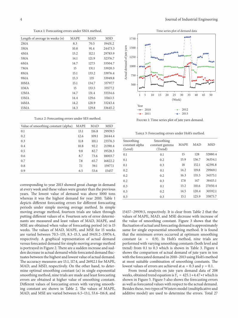
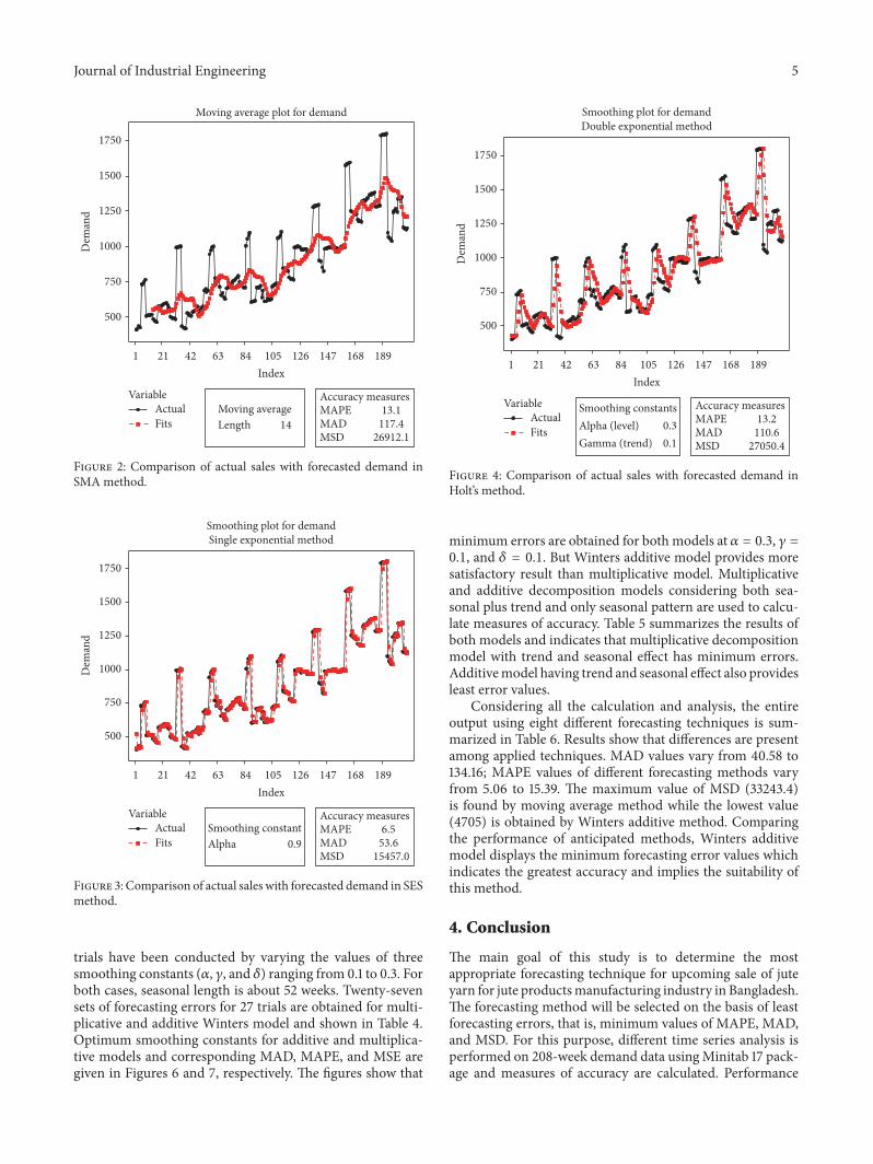
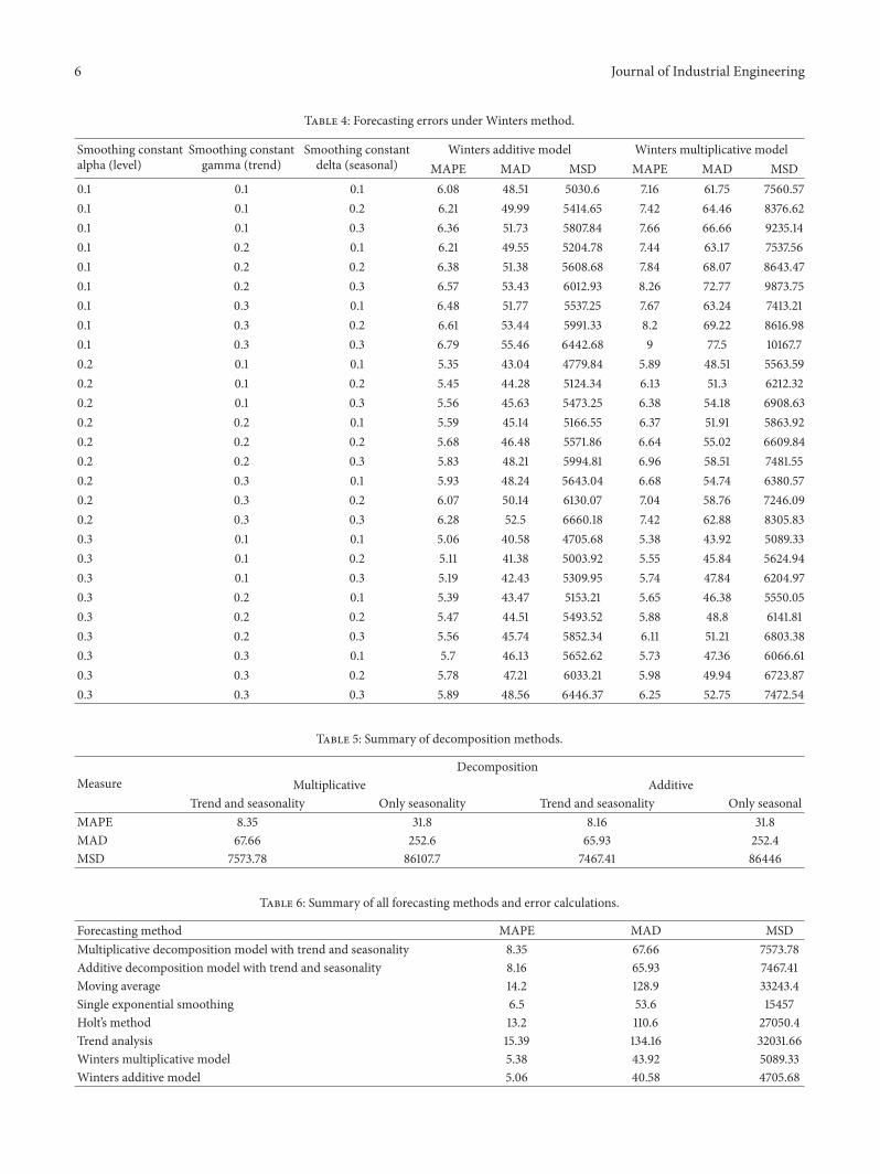
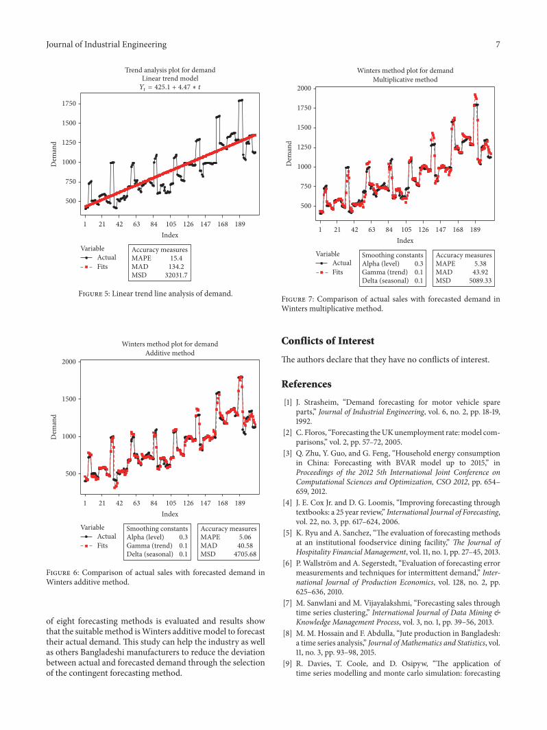


![Study on jute mill workers exposed to occupational hazardsiaimjournal.com/wp-content/uploads/2018/04/iaim_2018_0504_09.pdfMuralidhar Y, et al. [1] among the jute mill workers showed](https://static.fdocuments.net/doc/165x107/5e9c12ad9627d7740a6521fc/study-on-jute-mill-workers-exposed-to-occupational-muralidhar-y-et-al-1-among.jpg)