A Study of 2D Non-Stationary Massive MIMO Channels by ...

0018-9545 (c) 2020 IEEE. Personal use is permitted, but republication/redistribution requires IEEE permission. See http://www.ieee.org/publications_standards/publications/rights/index.html for more information.

This article has been accepted for publication in a future issue of this journal, but has not been fully edited. Content may change prior to final publication. Citation information: DOI 10.1109/TVT.2020.3037199, IEEETransactions on Vehicular Technology

1

A Study of 2D Non-Stationary Massive MIMOChannels by Transformation of Delay and Angular

Power Spectral DensitiesCarlos F. Lopez and Cheng-Xiang Wang, Fellow, IEEE

Abstract—In this paper, we propose a transformationmethod to model space-time-variant (STV) two-dimensionalnon-stationary wideband massive multiple-input multiple-output(MIMO) channels. This method enables us to obtain the STVjoint probability density function of the time of arrival and angleof arrival (AOA) at any time instant and antenna element of thearray from a predefined configuration of the scatterers. In addi-tion, we introduce a simplified channel modeling approach basedon STV parameters of the AOA distribution and demonstratethat key statistical properties of massive MIMO channels, suchas the STV temporal autocorrelation function and Doppler powerspectral density, can be derived in closed form. As examples ofapplication, we study multiple array-variant properties of threewidely-used geometry-based stochastic models (GBSMs): the Uni-fied Disk, Ellipse, and Gaussian scattering models. Furthermore,we present numerical and simulation results of the statisticalproperties of these three GBSMs and compare them with thoseobtained using the conventional spherical wavefront approach.We point out possible limitations of the studied channel modelsto properly represent massive MIMO channels.

Index Terms—Massive MIMO, non-stationary channel models,array-variant angular and delay distributions, transformationmethod, statistical properties.

I. INTRODUCTION

IN recent years, multiple-input multiple-output (MIMO)technologies have enabled a remarkable increase in reli-

ability, efficiency, and throughput of wireless communicationsystems by employing multiple antennas on one or both sidesof the communication link. Consequently, MIMO technologieshave widely been adopted in modern wireless communicationstandards. In particular, massive MIMO, i.e., MIMO tech-nologies incorporating a large number of antennas, has beenproposed as a solution to cope with the exigent requirements

This work was supported by the National Key R&D Program of China underGrant 2018YFB1801101, the National Natural Science Foundation of China(NSFC) under Grant 61960206006, the Frontiers Science Center for MobileInformation Communication and Security, the High Level Innovation andEntrepreneurial Research Team Program in Jiangsu, the High Level Innovationand Entrepreneurial Talent Introduction Program in Jiangsu, the ResearchFund of National Mobile Communications Research Laboratory, SoutheastUniversity, under Grant 2020B01, the Fundamental Research Funds for theCentral Universities under Grant 2242020R30001, and the EU H2020 RISETESTBED2 project under Grant 872172.

C.-F. Lopez is with The MathWorks, Glasgow, G2 2NR, U.K. (e-mail:[email protected]).

C.-X. Wang (corresponding author) is with the National Mobile Communi-cations Research Laboratory, School of Information Science and Engineering,Southeast University, Nanjing, 210096, China, and also with the PurpleMountain Laboratories, Nanjing 211111, China, and also with the Institute ofSensors, Signals and Systems, School of Engineering and Physical Sciences,Heriot-Watt University, Edinburgh, EH14 4AS, U.K. ([email protected]).

of the fifth-generation (5G) wireless communication systems[1]–[3]. Despite the great challenges caused by employinga large number of antennas, massive MIMO can providesubstantial gains as practical implementations have recentlydemonstrated [4]–[6]. However, important benefits of massiveMIMO technologies, e.g., increased array gain, angular resolu-tion, and diversity order, are intrinsically related to a sufficientseparation between adjacent antennas and the total size of theantenna array [7]. Thus, as packing many antennas in verycompact shapes is not always possible or desirable, massiveMIMO deployments often result in antenna arrays spanninglong distances, i.e., longer than the distance where the channelcan be considered wide-sense stationary (WSS).

In order to assess and design new wireless communica-tion technologies, it is of paramount importance to studyand model the underlying propagation channels. Large-scaleantenna arrays are subject to complex propagation effects, e.g.,near-field region effects, not present in conventional MIMOcommunication systems. These effects have been demonstratedby measurements and they include array-varying angle ofarrival (AOA), time of arrival (TOA), received power, andmultipath components (MPCs) (dis)appearance among others[8]–[16]. Consequently, massive MIMO channels can often notbe regarded as wide-sense stationary over the array [17].

In the past, time-domain non-WSS wireless channels werefirstly studied to enable high-mobility communication systems[18], [19], e.g., vehicular and high-speed train [20], [21], dueto their rapidly-varying characteristics. Recent high-mobilitychannel models [22], [23] employed the so called parametersdrifting, i.e., time-variant channel parameters such as TOAsand AOAs, with increased theoretical and computational com-plexity. Conversely, the family of COST channel models, e.g.,COST 207 [24] and COST 2100 [25], are intrinsically non-stationary in the time domain, but they determine the locationof the clusters of scatterers in the environment from thespecified angular and delay parameters and compute the exactdistance between the scatterers and transceivers. A similarapproach was used in recent works on massive MIMO channelmodeling that incorporated spherical [26]–[29] or parabolicwavefronts [30], [31]. Spherical and parabolic wavefrontscompute the exact and second-order approximations to thedistances between the scatterers and the antenna elementsof the array, respectively. Similarly to the parameters-driftingapproach, high-order wavefronts capture channel non-WSSproperties over the array at the expense of high theoreticaland computational complexity. However, channel models that

Authorized licensed use limited to: Southeast University. Downloaded on December 23,2020 at 14:08:12 UTC from IEEE Xplore. Restrictions apply.



2

can lead to closed-form expressions of their statistical prop-erties can help develop new techniques that improve systemperformance [32].

In [26], [28], [29], the authors proposed two-dimensional(2D) [26] and three-dimensional (3D) [28], [29] widebandmassive MIMO geometry-based stochastic models (GBSMs)that used spherical wavefronts, temporal parameter drifting,and space-time birth-death processes to capture near-fieldregion effects and (dis)appearance of clustered MPCs, re-spectively. In [31], a 3D wideband massive MIMO GBSMswere proposed, respectively, including parabolic wavefrontsof reduced complexity, cluster (re)appearance and shadowingprocesses in time and space domains. Whereas the authors in[26], [28], [31] neglected variations of the TOA over the array,[29] considered them. However, none of these works studiedthe space-time-variant (STV) distribution of TOA and AOA.

The quasi-deterministic channel models QuaDRiGa [33]and mmMAGIC [34] employed a combined approach includ-ing spherical wavefronts and temporal parameters drifting.The stochastic COST 2100 [25], METIS [35], 3GPP-NR[36] and IMT-2020 [37] channel models did not considerspherical wavefronts and supported mobility at the mobile-station side only. Although COST 2100 [25] channel modeldid not originally support large-scale arrays, an extension wasdeveloped in [38] to incorporate spherical wavefronts andvisibility regions over the array. The map-based deterministicMETIS model and the quasi-deterministic MiWEBA [39]channel model implicitly included spherical wavefronts andtemporal channel evolution through ray-tracing techniqueswith high computational complexity. Among these works,delay drifts over the array were only considered in QuaDRiGa[33], map-based METIS [35], and the extended COST 2100[38] models. However, these works [33], [35], [38] did notstudy the effects of delay drifts on the statistical properties ofmassive MIMO channels and none of the works above studiedthe STV distribution of TOA and AOA.

In [40], the authors employed the theory of transformationof random variables to investigate the spatial configuration ofthe scatterers in multiple coordinate systems for predefinedjoint probability density functions (PDFs) of the AOA andTOA. Similar investigations were conducted in the past forspecific GBSMs [41], [42], but they did not study non-WSSchannels in space or time domains.

In previous works [43], we reported preliminary results onthe delay drift over the array. However, we only studied theEllipse channel model and focused on the TOA variationsover the array, neglecting the spatial-temporal variations ofthe joint PDF of the TOA and AOA. Theoretical studies onthe STV joint PDF of the TOA and AOA and space-timeparameters drifting for non-WSS massive MIMO channelsare still missing. Moreover, the equivalence of the sphericalwavefront and parameters drifting approaches to model thestatistical properties of massive MIMO channels has not beeninvestigated yet. To fill these gaps, we propose a transfor-mation method to theoretically study spatial-temporal non-stationary wideband massive MIMO channels. The proposedmethod employs the theory of transformation of randomvariables and geometrical mappings in multiple coordinate

systems to model the STV joint PDF of the TOA and AOA forthe first time. It also enables us to obtain analytical expressionsof the STV scattering function (SF), delay and angular powerspectral densities (PSDs) for arbitrary configurations of thescatterers. In addition, we propose an approximation methodto obtain the STV angular spread, which was not considered inprevious theoretical studies of massive MIMO channels. Next,we highlight the contributions and novelties of this paper:

1) We propose a general transformation method to modelthe STV joint PDF of the TOA and AOA for 2D non-WSS massive MIMO channels. For the first time, wederive closed-form expressions of this joint-PDF forthe three most common ways of specifying the distri-bution of the scatterers, e.g., in the TOA-AOA, polar,and Cartesian domains, and for arbitrary-shaped 2Darrays. Through numerical evaluation and simulation, wedemonstrate the equivalence of the proposed methodsand the spherical-wavefront approach to capture thestatistical properties of the channel.

2) We obtain approximate expressions for the STV angularspread of the channel when the AOA follows a vonMises distribution. Additionally, we employ the STV an-gular spread to approximate new closed-form solutionsof key statistical properties of massive MIMO channels,such as the temporal autocorrelation function (ACF) andthe Doppler PSD.

3) We study the STV joint PDFs of the AOA and TOA ofwidely-used MIMO GBSMs such as the Ellipse, UnifiedDisk, and Gaussian scattering models. In all cases, weshow that the joint PDFs of the AOA and TOA aresubject to drifting and spreading over the array. Besides,we study the frequency correlation function (FCF) ofthese GBSMs and show that its array-varying propertiesare caused not only by the disappearance of MPCs, butalso by the drift and spread of the TOA over the array.

4) We describe some limitations of existing MIMO GBSMsthat were upgraded to simulate massive MIMO channels,e.g., the Unified Disk, Ellipse, and Gaussian scatteringmodels, due to the array-variant characteristics of thejoint PDF of the TOA and AOA.

The rest of this paper is organized as follows. In Section II,we present the non-stationary wideband massive MIMO chan-nel model employed in the following sections. In Section III,we derive the general transformation method for the threemost-used coordinate systems. Section IV applies the trans-formation method to widely-used MIMO channel models suchas the Ellipse or Gaussian cluster models. The derivation ofkey statistical properties of the channel from the transformedjoint PDF of the TOA and AOA is presented in Section V.In Section VI, we show the good agreement between thestatistical properties obtained through the proposed methodsand the spherical wavefront approach. Conclusions are drawnin Section VII.

II. A 2D WIDEBAND MASSIVE MIMO STOCHASTICCHANNEL MODEL

Let us consider a 2D wideband massive MIMO channelmodel depicted in Fig. 1 where the transmitter (Tx) and




3

receiver (Rx) are equipped with uniform linear antenna arrays(ULAs). The transmitting (receiving) ULA is composed ofNT (NR) omnidirectional antenna elements equally spacedwith a distance δT (δR) and it is tilted at an angle βT (βR)with respect to (w.r.t.) the x-axis of a Cartesian coordinatesystem centered at the receiving array’s center. The p-th (p =1, 2, ..., NT ) transmitting and q-th (q = 1, 2, ..., NR) receivingantenna elements are denoted by ATp and ARq , respectively. Weassume that the signal is omnidirectionally bounced only onceby each scatterer, denoted by Sn (n = 1, 2, ..., NS), and ittravels a distance Dn,qp(t) = DT

n,p +DRn,q(t) from ATp to ARq

via Sn at time instant t. Normally, the phase shifts θn intro-duced by the scatterers are modeled as independent and iden-tically distributed (i.i.d.) random variables obeying a uniformdistribution over [0, 2π) [44]. The massive MIMO channel isrepresented by the matrix H(t, τ) = [hqp(t, τ)]NR×NT whoseentries denote the channel impulse response (CIR) betweenthe antennas ATp and ARq . The CIR is given by

hqp(t, τ) =

NS∑n=1

cnejψn,qp(t)δ(τ − τn,qp(t)) (1)

where j =√−1, δ(·) is the Dirac delta function. The term

ψn,qp(t) = k0Dn,qp(t) + θn denotes the phase of the signal,k0 = 2π/λ, and λ denotes the carrier wavelength. The n-th scattered signal is received with amplitude cn and itsassociated propagation delay is τn,qp(t) = Dn,qp(t)/c0, wherec0 denotes the speed of light. Since signals from and tosufficiently separated antenna elements of the array experiencedifferent TOAs, τn,qp(t) in (1) depends on the antenna indicesp and q. The channel transfer function (CTF), i.e., the Fouriertransform of the CIR w.r.t. τ , is given by

Hqp(t, f) =

NS∑n=1

cnejψn,qp(t)e−j2πfτn,qp(t). (2)

For simplicity, we assume that the center of the receiving arrayis located at the origin at t = 0 and it moves at a constantspeed v forming an angle φv w.r.t. the x-axis. The Tx is staticand located at a distance d from the Rx along the negative x-axis. Accordingly, the distance traveled by the signal radiatedby ATp and received by ARq via Sn can be computed as

Dn,qp(t)=√

(xn − xRq − vxt)2 + (yn − yRq − vyt)2

+√

(xn + d− xTq )2 + (yn − yTp )2 (3)

Sn(xn, yn)

RxTx

x

y

d

v

φv

AT1

ATp

ATNT

AT2

δT

Sn+1Sn−1DT

n,p

DTn DR

n (t)AR

q

AR1

AR2

δR

ARNR

DRn,q(t)

βR

φRn

φTn

βT

Fig. 1. A 2D wideband massive MIMO channel model.

where (xn, yn) denote the Cartesian coordinates of Sn. Theterms xRq = δRq cos(βR) and yRq = δRq sin(βR) with δRq =(NR − 2q + 1)δR/2 denote the Cartesian coordinates of theantenna ARq at t = 0. Similarly, xTp = δTp cos(βT ) andyTp = δTp sin(βT ) with δTp = (NT − 2p + 1)δT /2 are theprojections of the position vector of ATp w.r.t. the center of thetransmitting array onto x and y axes, respectively. The Carte-sian components of the velocity vector are vx = v cos(φv) andvy = v sin(φv).

A. Spherical and Plane Wavefronts

Spherical wavefronts are considered in the model as longas (3) is used to compute the phase of the signal ψn,qp(t)in (1). The conventional approximation for short periods oftime and small arrays, i.e., the first-order or plane wavefrontapproximation, reduces the distance Dn,qp(t) to

Dn,qp(t)≈Dn − δTp cos(φTn − βT )

−δRq cos(φRn − βR)− vt cos(φRn − φv) (4)

where Dn = DTn +DR

n (0) =√

(xn + d)2 + y2n +

√x2n + y2

n

denotes the distance between the arrays’ centers, and theterms φTn and φRn denote the angle of departure (AOD)and AOA of the n-th scattered signal w.r.t. to the arrays’centers, which can be calculated as φRn = arctan(yn/xn) andφTn = arctan(yn/(xn + d)). Equation (4) can be obtained byreplacing δTp = xDT

n , δRq = yDRn (0), vt = zDR

n (0) in (3) andusing a first-order Taylor approximation of the two radicalswith respect to x, y, and z.

In spatial WSS non-massive MIMO channel models, theplane-wavefront approximation in (4) is usually employed tocompute the phase of the signal in (1) [44]. From (1) and (4),it can be seen that this approximation leads to linear space-time variations of the phase, which do not allow to capture thenon-WSS properties of massive MIMO channels. In addition,the TOA τn,qp(t) in (1) and (2) is usually approximated asa constant value for every scatterer, i.e., τn,qp(t) = τn. Thisassumption may be inaccurate for large antenna arrays.

III. A TRANSFORMATION METHOD OF THE STV JOINTPDF OF THE TOA AND AOA

In conventional WSS GBSMs [44], scatterers are assumedto be randomly distributed in the environment according to apredefined PDF that models the TOA and AOA of the receivedsignal, and this PDF is space-time-frequency independent [40].Unlike WSS channels, measurements [8]–[16] have shown thatTOAs and AOAs may change over the array and time for largearrays and periods of time, respectively. In this section, weintroduce a method based on the transformation of randomvariables to obtain the STV joint PDF of TOA-AOA forevery antenna pair ATp –ARq at any time instant t. The methodproposed is developed for the three most common domainsused to specify the distribution of the scatterers: TOA-AOA,Polar, and Cartesian domains.




4

A. Transformation in TOA-AOA Domain

For clarity, the most important elements of the TOA-AOAtransformation are illustrated geometrically in Fig. 2 for aMIMO system employing 2×2 antennas at time instant t = 0.Note that we have depicted ULAs for convenience, but theproposed method is not limited to any arrangement of theantenna arrays, i.e., it can be applied to arbitrary-shaped 2Darrays. The origins of the Cartesian coordinate systems (X,Y )and (X1, Y1) are located at the center of the receiving arrayand AR1 , respectively. The AOAs of the signal scattered bySn and measured at (X,Y ) and (X1, Y1) are denoted by φRnand φR1,n, respectively. Signals radiated from the center of thetransmitting array and bounced by the scatterers located in theellipse ε, e.g., Sj and Sn, arrive at the center of the receivingarray with the same TOA, which is denoted as τn. Likewise,the ellipse ε1 illustrates the same concept as ε when the signalstransmitted from AT2 and received at AR1 experience a constantdelay denoted as τ1,n.

The direct transformation of the random TOA and AOAmeasured at the center of the array (τ, φR) to the TOA andAOA measured at any antenna element and time instant t(τ1, φ

R1 ) is defined as

τ =c−10

(√x2 + y2 +

√(x+ d)2 + y2

)(5)

φR = arctan(y/x) (6)

with

x =1

2

[(c0τ1)2 − d2

qp(t)

c0τ1 + dqp(t) cosφR1

]cos(φR1 + αqp(t)) + xRq + vxt (7)

y =1

2

[(c0τ1)2 − d2

qp(t)

c0τ1 + dqp(t) cosφR1

]sin(φR1 + αqp(t)) + yRq + vyt. (8)

The parameter dqp(t) denotes the distance between ATp andARq and αqp(t) the angle between the segment joining ATpand ARq and the x-axis at time instant t. These parameters arecalculated in Appendix A.

RxTx

Snǫ

AR1

AR2

AT1

AT2

dqp

Y1

X1

ǫ1

X

Y

d

τn

τ1,n

φRn

φR1,n

βT βRv φv

Sj

Sk

φTn

Fig. 2. Elements of the transformation of the joint PDF of the TOA and AOAat t = 0.

As the direct transformation of the random TOA and AOAis rather complicated and leads to cumbersome expressionsfor the Jacobian determinant, we use a stepped approach toobtain the STV joint PDF of TOA-AOA. The distribution ofthe TOA-AOA of a signal radiated from AT2 and received atAR1 can be obtained using the following steps:

1) From a given distribution of TOA-AOA fτ,φR(τ, φR),the joint PDF of the location of the scatterers fXY (x, y)in the Cartesian coordinates (X,Y ) is derived as pro-posed in [40]. The transformation of the random vari-ables (τ, φR) is indeed a transformation of coordinates.

2) A second transformation is performed from (X,Y ) into(X1, Y1), resulting in the PDF fX1Y1(x1, y1). Thesetwo coordinate systems are related by shift and rotationoperations according to the relative positions of theantennas AT2 and AR1 .

3) The locations of the scatterers in the system (X1, Y1) aretransformed back into the TOA-AOA domain, obtainingthe PDF fτ1,φR1 (τ1, φ

R1 ) for the antenna elements AT2

and AR1 .Using the previous approach, the joint PDF can be obtainedas (see Appendix A)

fτ1,φR1 (τ1, φR1 )=

(|J1(x, y)||J3(τ1, φ

R1 )|)−1

fτ,φR(τ, φR) (9)

where τ and φR were obtained in (5)–(8), respectively. TheJacobian determinants J1(x, y) and J3(τ1, φ

R1 ) can be found

in Appendix A. Notice that the actual AOA measured fromARq is not φR1 but φR1 − αqp(t) due to the rotation of thecoordinate system (X1, Y1) w.r.t. (X,Y ). It can be seenthat for small arrays and periods of time, i.e., δTMT

�(c0τ − d), δRMR

� (c0τ − d), and vt � (c0τ − d), then|J1(x, y)|−1|J3(τ1, φ

R1 )|−1 ≈ 1, αqp(t) ≈ 0, dqp(t) ≈ d, and

fτ1,φR1 (τ1, φR1 ) ≈ fτ,φR(τ, φR). Thus, when the joint PDF of

TOA-AOA is independent of the antenna element and timeinstant, the channel can be considered as WSS.

The main advantage of this stepped approach compared tothe direct one from (τ, φR) to (τ1, φ

R1 ) is that the equations

of the Jacobian determinants J1 and J3 can be reused forother specifications of the scatterers’ distribution in differentdomains such as (14) and (15). In addition, the expressions forthe Jacobian determinants of the transformations are simpler.

It is important to highlight the difference between thetransformation method proposed and the ones used in pre-vious theoretical works (e.g., [45]–[47] and [26]–[28]). In theproposed method, the parameters that define fτ,φR(τ, φR) arespace-time invariant, but this distribution gets transformed fordifferent antenna elements of the arrays and time instants.In those previous works, it was assumed that only someparameters, e.g., the mean AOA, defining the distribution areSTV, but the distribution remained space-time invariant. Theprevious approach is an approximation that may only hold insome limited cases as we will show in subsequent sections.

B. Transformation in Polar Domain

Analogous to the previous section, the PDF of the po-sition of the scatterers is transformed in three steps. How-ever, as the given PDF is defined in polar coordinates, i.e.,




5

fR,φR(r, φR), the first transformation of the random variables(r, φR) to (X,Y ) is performed using X = R cos(φR) andY = R sin(φR). The joint PDF of (X,Y ) is given by

fX,Y (x, y) = |J1(x, y)|−1fR,φR(r, φR) (10)

where

r =√x2 + y2 (11)

φR =arctan(y/x) (12)

and J1(x, y) is the Jacobian of the transformation, i.e.,

|J1(x, y)|−1 =

∣∣∣∣∣ 1√x2 + y2

∣∣∣∣∣ . (13)

Finally, the joint PDF of (τ1, φR1 ) can be obtained as

fτ1,φR1 (τ1, φR1 )=

(|J1(x, y)||J3(τ1, φ

R1 )|)−1

fR,φR(r, φR) (14)

where |J3(τ1, φR1 )|−1, x, and y are defined in (45), (7), and

(8), respectively.

C. Transformation in Cartesian Domain

In this case, the transformation procedure is reduced to twosteps as it is not necessary to perform a transformation toCartesian coordinates. Thus, the joint PDF fτ1,φR1 (τ1, φ

R1 ) is

a function of the joint PDF fX,Y (x, y) and is obtained as

fτ1,φR1 (τ1, φR1 ) =

∣∣∣J3(τ1, φR1 )∣∣∣−1

fX,Y (x, y) (15)

where x and y are defined in (7) and (8), respectively.

IV. APPLICATION OF THE TRANSFORMATION METHOD TOMIMO CHANNEL MODELS

In this section, the transformation method described inSection III is applied to study the TOA-AOA variations acrossthe array of widely-used channel models defined in each of thethree different domains. For the TOA-AOA domain, the Ellipsenarrowband and wideband channel models are studied. For thePolar domain, the one-ring model and unified disk scatteringmodel (UDSM) are analyzed. For the Cartesian domain, theGaussian cluster channel model is employed.

1) Ellipse Narrowband and Wideband Channel Models:In the Ellipse channel model, the scatterers are located inthe perimeter of an ellipse with foci at the center of thetransmitting and receiving arrays. In the single-ellipse model,the TOA is fixed to a single value τ0, but the AOA distributionis not defined. In this paper, we will employ the von Misesdistribution to model the AOA as an example, as it can coverboth isotropic and non-isotropic angular distributions throughits parameters [44], [48]. For large values of its concentrationparameter κ, the von Mises distribution accurately approxi-mates a Gaussian distribution, which has been widely reportedand used in standard-based channel models such as 3GPP-NR[36]. The joint PDF is given by

fτ,φR(τ, φR) = δ(τ − τ0) · 1

2πI0(κ)eκ cos(φR−µφ) (16)

where µφ and κ are the mean AOA and concentration param-eter, respectively, and I0(·) denotes the zero-order modifiedBessel function of the first kind. It is important to remarkthat (16) implies independent time dispersion and frequencydispersion [44], i.e., its joint PDF of TOA-AOA is separable,and is also a narrowband channel model, i.e., the absolutevalue of the FCF is constant. A more flexible distribution thatincludes the previous one as a special case and permits tocapture wideband characteristics of the channel is

fτ,φR(τ, φR) =e−

(τ−τ0)στ

στu(τ − τ0)

1


where u(·) denotes the unit-step function, i.e., u(x) = 1 forx > 0 and zero otherwise. Note that the marginal distributionof delays δ(τ − τ0) in (16) has been substituted in (17) bya shifted exponential distribution with minimum delay τ0 andstandard deviation στ , which denotes the delay spread of thechannel. The unit-step function is used to guarantee that themodel is causal. It is clear that as στ → 0, the PDF in (17)converges to that in (16). From the communications system’sperspective, as long as στ is much smaller than the time-resolution of the system considered, both distributions modelequivalent channels. The transformed PDFs at the antennasATp , ARq and time instant t can be obtained by plugging (16)and (17) into (9). As it will be shown in the results presentedin Section VI, the transformation of (16) breaks down theseparability of the distribution of TOA-AOA, introducing adependence between these two random variables. This canbe easily seen by noting that the term δ(τ − τ0) in (16) istransformed into δ(c−1

0 [√x2 + y2 +

√(x+ d)2 + y2] − τ0),

with x and y given by (7) and (8), respectively. As thevalues of φR1 that solve

√x2 + y2 +

√(x+ d)2 + y2 = c0τ0

depend on the the delay τ1, the TOA and AOA are dependentand therefore correlated. As this argument can be appliedto any separable distribution, the important independent timedispersive and Doppler frequency dispersive property [44] ofthe Ellipse and other channel models is broken down by thelarge dimensions of the array.

2) One-Ring model and Unified Disk Scattering Model(UDSM): The One-Ring model defines the geometrical config-uration of the scatterers in a circular ring around the center ofthe receiving array. This geometry is usually applied to modelnarrowband channels, although its delay spread is not zero andvaries according to the radius of the ring and the distribution ofthe AOA [49]. Using the von Mises distribution for the AOA,the PDF of the position of the scatterers in polar coordinatesis given by

fR,φR(r, φR) = δ(r − r0) · 1


where r0 is the radius of the ring. A more flexible distributionthat includes the one-ring model as a special case is the UDSM[50]. Although the UDSM is constrained to uniform distribu-tions of the AOA, the PDF of the position of the scatterers




6

can be extended to account for non-uniform distributions as

fr,φR(r, φR)=(kU + 1)

r(kU+1)0

rkU ·[u(r)− u(r − r0)

]× 1


where kU > −1 is a real-valued parameter called the shapefactor that controls the spread of the scatterers w.r.t. theradial distance. As kU → ∞, the scatterers become moreconcentrated near the edge of the disk forming a ring ofradius r0 and (19) converges to (18). The transformed PDFsat the antennas ATp , ARq and time instant t can be obtainedby plugging (18) and (19) into (14). The resulting PDFs areomitted here for brevity.

3) Gaussian Cluster Channel Model: The Gaussian clustermodel has widely been used in multiple standard GBSMs,e.g., COST 207 [24] and COST 2100 [25], to model single-and multi-bounce clustered MPCs including intracluster delayand angle spreads. A simplified PDF of the position of thescatterers for this model in Cartesian coordinates is given by

fX,Y (x, y) =1

2πσ2xy

e−1

2σ2xy[(x−x0)2+(y−y0)2]

(20)

where (x0, y0) denote the coordinates of the center of thecluster and σxy the spread of the cluster in the xy-plane. Notethat the spreads of the cluster in the x and y axes are assumedto be equal here for simplicity. The joint PDF fτ1,φR1 (τ1, φ

R1 )

can be obtained by plugging (20) into (15). The resulting PDFis omitted here for brevity.

V. STATISTICAL PROPERTIES OF MASSIVE MIMOCHANNELS

In the following, the STV PDF fτ1,φR1 (τ1, φR1 ) obtained

in Section III will be used to compute the STV statisticalproperties of the channel such as the Doppler, delay, andangular PSDs, and the space-time-frequency cross-correlationfunction (STF-CCF).

A. Computation of Statistical Properties from the TransformedDistribution of the TOA-AOA

1) Delay PSD: The delay PSD or power delay profile(PDP) is a measure of the distribution of the received power inthe delay domain. It can be seen that the PDP is proportionalto the distribution of the TOA of the received signal [44, p.348]. Accordingly, the STV PDP can be obtained through themarginal PDF of τ1 as Sτ1(τ1) = σ2

0fτ1(τ1) where σ20 denotes

the total received power and fτ1(τ1) denotes the marginal PDFof the TOA.

2) Angular PSD: Similarly, the angular PSD or powerangular spectrum (PAS) is a measure of the incoming powerin the angular domain. Thus, the STV PAS can be analo-gously obtained through the marginal PDF of the AOA φR1 asSφR1 (φR1 ) = σ2

0fφR1 (φR1 ) where fφR1 (φR1 ) denotes the marginalPDF of the AOA.

3) Doppler PSD: For a mobile station moving at a constantspeed v and direction defined by the angle φv , and a set ofstatics scatterers, the Doppler frequency ν is a function of theAOA as ν = νmax cos(φR1 − φv), where νmax = v/λ denotesthe maximum Doppler frequency. According to this definition,it can be proved that the Doppler PSD is given by [44]

Sν(ν)=2σ0

νmax√

1− (ν/νmax)2gφR1 (arccos[ν/νmax]) (21)

where

gφR1 (φR1 ) =1

2

(fφR1 (φR1 ) + fφR1 (−φR1 )

)(22)

is the even part of the STV PDF of the AOA.4) Space-Time-Frequency Cross-Correlation Function

(STF-CCF): In the proposed approach, the cross-correlationbetween the signal corresponding to the link ATp –ARq attime instant t and frequency f , and that of the link ATp′–A

Rq′

at time t + ∆t and frequency f + ∆f can be obtained asρqp,q′p′(t,∆t,∆f) = E[Hqp(t, f)H∗q′p′(t+ ∆t, f + ∆f)],with E(·) denoting the expectation operator and H∗ thecomplex conjugate of H . Thus, the STF-CCF can becomputed as

ρqp,q′p′(t,∆t,∆f) = σ20

∫ ∞0

∫ 2π

0

e−jk0Ψq′p′qp (t,∆t)e−j2π∆fτ1

×fτ1,φR1 (τ1, φR1 )dτ1dφR1 (23)

where Ψq′p′

qp (t,∆t) = ∆pp′ cos(φT1 − βT + αqp(t)) +∆qq′ cos(φR1 − βR + αqp(t)) + v∆t cos(φR1 − φv + αqp(t))denotes the phase difference between the signal transmittedfrom ATp and received by ARq at time t and the signaltransmitted from ATp′ and received by ARq′ at t + ∆t. Thedistance between ATp and ATp′ is ∆pp′ = (p− p′)δT , and thatbetween ARq and ARq′ is ∆qq′ = (q− q′)δR. It is worth notingthat near-field region effects, which are usually modeled usingspherical wavefronts, are captured in the proposed method bythe space-time variant PDF of the TOA and AOA.

When the spherical wavefront is used, the STF-CCF can becalculated as [27]

ρqp,q′p′(t,∆t,∆f) = σ20

∫ ∞0

∫ 2π

0

e−jk0Ψq′p′qp (t,∆t)e−j2π∆fτ

×fτ,φR(τ, φR)dτdφR (24)

where Ψq′p′

qp (t,∆t) = Dqp(t) − Dq′p′(t + ∆t) and Dqp(t)denotes the total distance traveled by the signal from ATp toARq at time instant t as given by (3). Notice that the TOA andAOA used in (24) are defined at the center of the transmittingand receiving arrays at time t = 0 and they are space-timeinvariant. Consequently, the spherical wavefront is requiredto capture non-WSS properties of the channel and the planewavefront approximation in (4) cannot be used.

With respect to the deterministic simulation model as de-fined in (1) and (2) once the random variables involved aredrawn, the STF-CCF can be approximated as a local time-average, i.e.,

ρqp,q′p′(t,∆t,∆f) ≈ 1

T

∫ t2

t1

Hqp(t′, f)

×H∗q′p′(t′ + ∆t, f+∆f)dt′ (25)




7

where t1 = t − T/2 and t2 = t + T/2. The temporal ACFscan be obtained by setting ∆f = ∆qq′ = ∆pp′ = 0 in(23), (24), and (25) as ρqp,qp(t,∆t, 0), ρqp,qp(t,∆t, 0), andρqp,qp(t,∆t, 0), respectively. By setting ∆t = ∆f = 0 in thesame equations, we can calculate the spatial cross-correlationfunctions (S-CCFs) as ρqp,q′p′(t, 0, 0), ρqp,q′p′(t, 0, 0), andρqp,q′p′(t, 0, 0). The FCFs are computed by setting ∆qq′ =∆pp′ = ∆t = 0 as ρqp,qp(t, 0,∆f), ρqp,qp(t, 0,∆f), andρqp,qp(t, 0,∆f). The ACFs, S-CCFs, and FCFs obtained de-pend on the antenna indices and the time instant through τ1and φR1 in (23) and through the total distance in Ψq′p′

qp (t,∆t)in (24), indicating that the channel is space-time non-WSS.

B. Approximate Solutions to the ACF and Doppler PSD

Although analytic solutions for the STF-CCF in (23) aredifficult to obtain due to the complexity of the STV joint PDFof the TOA and AOA, approximate expressions for the ACF,Doppler PSD, and S-CCF can be derived for non-WSS massiveMIMO channels. We propose a simplified approach based onan implicit assumption of previous works, e.g., [51] and [45],in which the PAS was assumed space-time invariant, but someof its parameters were not.

Let us consider that the AOA defined at the center of thearray (φR) follows a von Mises distribution with parameters(κ, µφ). Then, if we assume that only the parameters of thisdistribution are STV, the PDF of the AOA for any ATp , ARqand time instant t becomes

fφR1 (φR1 ) =1

2πI0(κqp(t))eκqp(t) cos(φR1 −µ

φqp(t)) (26)

where the mean AOA µφqp(t) and concentration parameterκqp(t) are now dependent of time and antenna indices. Inslowly varying channels, we can assume that the rates ofchange of µφqp(t) and κqp(t) are small. Consequently, theseparameters can be considered approximately constant for shortintervals of the array and periods of time. If the spatial-temporal evolution of these parameters is known, the STVACF can be approximated as [44]

ρ(∆t; δTp , δ

Rq ,t) ≈

2σ20

I0(κqp(t))I0

([κ2qp(t)− (2πνmax∆t)2

−j4πκqp(t)νmax∆t cos(µφqp(t)− φv))] 1

2

). (27)

As the parameters µφqp(t) and κqp(t) depend on the positionover the array and time instant, the channel is non-WSS inthese domains. Similarly, according to (21), the STV DopplerPSD is

Sν(ν)≈ 2σ20 e

κ2qp(t) cos(µφqp(t)−φv)ν/νmax

πνmaxI0(κ2qp(t))

√1− (ν/νmax)2

× cosh(κ2qp(t) sin(µφqp(t)− φv)

√1− (ν/νmax)2

). (28)

In Appendix B, we derive approximate solutions of the STVconcentration κqp(t) and mean AOA µφqp(t) as

κqp(t)=κ

1 +

(δRqrc

)2

+

(vt

rc

)2

− 2δRqrc

cos(µφc − βR)

−2vt

rccos(µφc − φv) + 2

vtδRqr2c

cos(βR − φv)

)(29)

and

µφqp(t) = arctan(ξ) (30)

with

ξ =rc sin(µφc )− δRq sin(βR)− vt sin(φv)

rc cos(µφc )− δRq cos(βR)− vt cos(φv). (31)

It can be easily seen that, for small arrays and short periodsof time, i.e., MRδR/2 � rc and vt � rc, the concentrationparameter and mean AOA become invariant, i.e., κc,q(t) ≈ κcand µφqp(t) ≈ µφc .

VI. RESULTS AND ANALYSIS

In this section, we will present and compare the array-variant distribution of channel parameters and statistical prop-erties obtained using the proposed transformation method,approximation method, spherical wavefront approach, andsimulation results, for three channel models introduced inSection III. The results corresponding to the transformationmethod were obtained by numerical evaluation of (9), (14),and (15). Similarly, those corresponding to the approximationmethod were computed by evaluating (27)–(28) and makinguse of the variant parameters as determined by (29) and (30).We evaluated (24) to obtain the results corresponding to thespherical wavefront approach. For the simulation results, wegenerated 103 scatterers randomly distributed and computedthe CIR as in (2). Realizations of the channel parameters,e.g., TOA and AOA, were obtained by the inverse transformsampling method [52]. To obtain the simulation results, thestatistical properties were computed by averaging 103 realiza-tions of the STF-CCF in (25).

In the following, we assume that no line-of-sight path existsbetween the Tx and Rx, which are located 100 m apart alongthe x-axis at t = 0 and both count on ULAs composed of100 antenna elements each. The separation between adjacentantennas is λ/2 at 2 GHz of carrier frequency.

A. Array-Variant TOA-AOA joint PDF

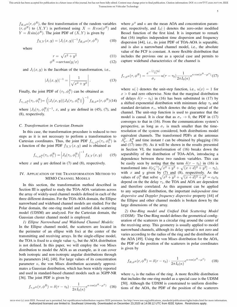
In Fig. 3, we present the STV joint PDFs of the TOA-AOA in logarithmic scale (dB) of the wideband Ellipse channelmodel at the extremes and center of the receiving array, i.e.,at AR1 (left), AR50 (center), and AR100 (right). We imposed aminimum TOA of τ0 = 400 ns and a von Mises concentrationparameter k = 0, i.e., uniform scattering in the AOA.

On one hand, the joint PDF of the TOA-AOA at AR50

(center) shows the properties imposed by the channel modelsuch as uniformity in the AOA domain, exponential decay inthe TOA domain, and independence between TOA and AOA.




8

On the other hand, the PDFs at the extremes of the arrayare remarkably affected by the transformation. The resultingmeandering shape of the PDFs at AR1 and AR100 shows that theTOA varies as a function of the AOA. This is most noticeablewhen the receiving antenna is far from the focus of the ellipse,i.e., at AR1 and AR100, as the sum of the distances from theopposite focus (Tx) to such antennas via scatterers of theellipse is highly variant. In the AOA domain, the uniformityimposed (κ = 0) at the center of the array is no longer valid atits ends. Two maxima of the PDF appear around φR1 ≈ −π/2and φR1 ≈ π/4 for AR1 and AR100, respectively, indicating areduction of the angular spread.

These results show that, at the extremes of a large-scalearray, additional delay spread may be introduced into thechannel model with unforeseen consequences. This artifact ofthe Ellipse channel model produced by the large dimensions ofthe array was not considered in previous works, e.g., [26]–[28],[30], [31]. Moreover, Fig. 3 indicates that the transformationperformed breaks down the separability of the joint PDF ofthe TOA and AOA, as the conditional distribution of the AOAgiven a specific TOA depends on the delay considered.

As the STV statistical properties of the channel are notice-able only when the scatterers are relatively close to any ofthe arrays, we will use the parameters of the channel modelspresented in Table I in the following unless otherwise stated.The parameters of the Ellipse, modified UDSM, and Gaussiancluster models are selected so that the maximum concentra-tions of the scatterers of all three models are coincident. Thedelay spread of the Ellipse model στ and distance spread ofthe UDSM model σr can be chosen arbitrarily small.

B. Array-Variant Delay and Angular PSDs

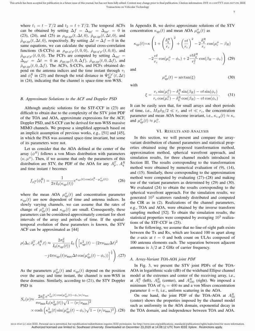
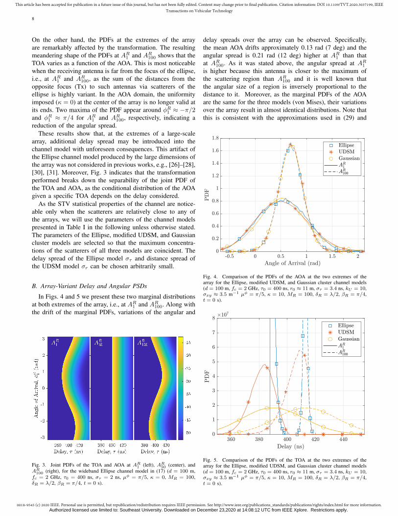
In Figs. 4 and 5 we present these two marginal distributionsat both extremes of the array, i.e., at AR1 and AR100. Along withthe drift of the marginal PDFs, variations of the angular and

Fig. 3. Joint PDFs of the TOA and AOA at AR1 (left), AR50 (center), andAR100 (right), for the wideband Ellipse channel model in (17) (d = 100 m,fc = 2 GHz, τ0 = 400 ns, στ = 2 ns, µφ = π/5, κ = 0, MR = 100,δR = λ/2, βR = π/4, t = 0 s).

delay spreads over the array can be observed. Specifically,the mean AOA drifts approximately 0.13 rad (7 deg) and theangular spread is 0.21 rad (12 deg) higher at AR1 than thatat AR100. As it was stated above, the angular spread at AR1is higher because this antenna is closer to the maximum ofthe scattering region than AR100 and it is well known thatthe angular size of a region is inversely proportional to thedistance to it. Moreover, as the marginal PDFs of the AOAare the same for the three models (von Mises), their variationsover the array result in almost identical distributions. Note thatthis is consistent with the approximations used in (29) and

Fig. 4. Comparison of the PDFs of the AOA at the two extremes of thearray for the Ellipse, modified UDSM, and Gaussian cluster channel models(d = 100 m, fc = 2 GHz, τ0 = 400 ns, r0 ≈ 11 m, στ = 3.4 ns, kU = 10,σxy ≈ 3.5 m−1 µφ = π/5, κ = 10, MR = 100, δR = λ/2, βR = π/4,t = 0 s).

Fig. 5. Comparison of the PDFs of the TOA at the two extremes of thearray for the Ellipse, modified UDSM, and Gaussian cluster channel models(d = 100 m, fc = 2 GHz, τ0 = 400 ns, r0 ≈ 11 m, στ = 3.4 ns, kU = 10,σxy ≈ 3.5 m−1 µφ = π/5, κ = 10, MR = 100, δR = λ/2, βR = π/4,t = 0 s).




9

TABLE IPARAMETERS OF THE PDFS OF THE THREE CHANNEL MODELS.

Ellipse UDSM Gaussian

φR (rad) τ (ns) φR (rad) r (m) X (m) Y (m)

µφ σφR µτ στ µφ σφR µr σr µX σX µY σYπ5

π10

400 1 π5

π10

11 1 8.9 3.5 6.4 3.5

(30) to obtain the STV parameters of the AOA distribution.Although each model presents a different marginal PDF of theTOA, a similar drift of approximately 23 ns of the mean TOAand small variations of the delay spread (below 1 ns) can beobserved in Fig. 5 for the three models.

C. Array-Variant ACF

In Fig. 6, we present a comparison of the absolute valuesof the array-variant local ACFs obtained by the transformationmethod, approximation method, spherical wavefront approach,and simulation, at the two extremes of the receiving ULAand for different directions of motion φv . Although there aresmall differences between the results corresponding to eachmethod, the ACFs obtained through the transformation andapproximation methods are very similar in the whole range.Moreover, the good agreement between the methods proposedand the spherical wavefront approach indicates that all thesemethods are approximately equivalent. Note that only the ACFof the Ellipse model is presented in Fig. 6. This is becausein equal conditions of motion, i.e., v and φv are equal forthe three models, the ACF is only determined by the PDF ofthe AOA. As the PDFs of the AOA of the three models areapproximately equal as shown in Fig. 4, it is not necessary toshow the ACFs corresponding to the other models.

Fig. 6. Comparison of the absolute values of the local ACFs obtained by thetransformation method, approximation method, spherical wavefront approach,and simulation at the two extremes of the receiving array (d = 100 m,fc = 2 GHz, τ0 = 400 ns, στ = 3.4 ns, µφ = π/5, κ = 10, MR = 100,δR = λ/2, βR = π/4, νmax = 90 Hz, v = 13.5 m/s, δT = 0 m, t = 0).

Fig. 7. Comparison of the absolute values of the local Doppler PSDs obtainedby the transformation method, the approximation method, and simulation atthe two extremes of the receiving array (d = 100 m, fc = 2 GHz, τ0 = 400ns, στ = 3.4 ns, µφ = π/5, κ = 10, MR = 100, δR = λ/2, βR = π/4,νmax = 90 Hz, v = 13.5 m/s, δT = 0 m, t = 0).

D. Array-Variant Doppler PSD

In Fig. 7, we present a comparison of the absolute valuesof the array-variant Doppler PSDs obtained through the trans-formation method, the approximation method, the sphericalwavefront approach, and simulation, at the two extremes of theULA and for different directions of motion φv . The variationsof the Doppler PSD along the array can be attributed to thedifference in relative motion w.r.t. the scatterers at sufficientlyseparated antenna elements, e.g., AR1 and AR100. It can be seenthat not only the Doppler PSD drifts along the array, but alsothe Doppler spread is affected. On one hand, when the ULApoints to the maximum concentration of the scatterers, i.e.,βR−µφ ≈ 0 or βR−µφ ≈ π, the Doppler PSD hardly drifts,but there is a noticeable variation of the Doppler spread alongthe array. On the other hand, for a perpendicular orientationof the ULA, i.e., when βR − µφ ≈ ±π/2, the Doppler PSDdrifts over the array, but the Doppler spread hardly varies.

E. Array-Variant S-CCF

In Fig. 8, we present a comparison of the absolute valuesof the array-variant receive-side S-CCFs obtained by using thetransformation method, the approximation method of variantparameters, the spherical wavefront approach, and simulation,at the receive antenna positions AR1 and AR100 for differentvalues of the angular tilt of the receiving antenna βR. Thereis clearly a good agreement between the transformation and




10

Fig. 8. Comparison of the absolute values of the local S-CCFs obtained bythe transformation method, the approximation method, the spherical wavefrontapproach, and simulation at the two extremes of the receiving array (d = 100m, fc = 2 GHz, τ0 = 400 ns, στ = 3.4 ns, µφ = π/5, κ = 10, MR = 100,δR = λ/2, βR = π/4, δT = 0 m, t = 0 s).

approximation methods proposed. The differences between thetransformation and approximation methods can be attributedto the fact that the latter assumes that the function determiningthe PAS remains the same, e.g., von Mises (26), at any positionof the array and only the parameters of that function, i.e., κand µφ, are array-variant.

F. Array-Variant FCF

In Fig. 9, the absolute values of the array-variant FCFs ofthe Ellipse, modified UDSM, and Gaussian cluster modelsare presented. In the figure, it can be seen that the variantdistribution of the TOA results in array-variant FCFs as aconsequence of the large dimensions of the receiving array.This effect is specially significant for the modified UDSMand the Ellipse model. In the last one, the imposed nar-rowband property (στ = 0.3 ns) or frequency flatness isslowly degraded as the distance between the center of thearray and the considered antenna element increases. The causeof this artifact has already been explained in the analysisof Fig. 3. As a consequence, what it was designed as afrequency non-selective and frequency-uncorrelated channelmodel may change to a frequency-selective and frequency-correlated channel for sufficiently large arrays. Note that inthe case of the Ellipse model we have chosen a sufficientlysmall value of the delay spread στ to consider the channelas frequency non-selective in most practical cases, as it canbe seen in the almost-flat FCF depicted for AR50. Conversely,the FCF of the Gaussian cluster model is barely affected asthe shift and rotation of a 2D symmetric Gaussian distributiononly affects its mean values, but not its spread. Hence, itsdelay PSD only experiences a shift (see Fig. 5), which affectsthe phase but not the absolute value of the FCF.

VII. CONCLUSIONS

In this paper, we have proposed a novel method to modelthe joint PDF of the TOA and AOA in massive MIMOchannels. The proposed method can be used to study massiveMIMO channel characteristics of both channel measurementsand models. We have also proposed an approximation methodbased on varying angular parameters for the von Mises dis-tribution and obtained approximate closed-form expressionsof key statistical properties of the channel. The statisticalproperties obtained with these two methods have shown agood agreement between them and with the spherical wave-front approach. The proposed methods incorporated the non-stationary properties of the channel model through the jointPDF of the TOA and AOA. Moreover, we showed that themeans and spreads of the AOA and TOA vary over the array.Due to the delay drift and spread, we demonstrated that theFCF of massive MIMO channels is array-variant as well.Finally, it has been demonstrated that artifacts may appearwhen conventional MIMO models such as the Ellipse modeland UDSM are applied to large-scale arrays.

APPENDIX ATRANSFORMED PDF OF THE TOA AND AOA

For single-bounced rays, the TOA-AOA parameters of therays (τ, φR) are related to their Cartesian coordinates in(X,Y ) through the following non-linear transformation equa-tions [40]

X =1

2

(c0τ)2 − d2

c0τ + d cosφRcosφR (32)

Y =1

2

(c0τ)2 − d2

c0τ + d cosφRsinφR. (33)

The PDF in Cartesian coordinates can be calculated by apply-ing the theory of transformation of random variables as [40]

Fig. 9. Comparison of the absolute values of the local FCFs at AR1 and AR50obtained by the transformation method, the spherical wavefront approach, andsimulation (d = 100 m, fc = 2 GHz, τ0 = 400 ns, r0 ≈ 11 m, στ = 0.3ns, kU = 10, σxy ≈ 3.5 m−1, µφ = π/5, κ = 10, MR = 100, δR = λ/2,βR = π/2, δT = 0 m, t = 0 s).




11

fX,Y (x, y) = |J1(x, y)|−1fτ,φR(τ(x, y), arctan(y/x)

)(34)

with τ(x, y) = c−10 (√x2 + y2 +

√(x+ d)2 + y2). J1(x, y)

is the Jacobian of the transformation, i.e.,

|J1(x, y)|−1 = c−10

∣∣∣∣∣∣ 1√x2 + y2

+1 + dx

x2+y2√(x+ d)2 + y2

∣∣∣∣∣∣ . (35)

Using fX,Y (x, y), we can obtain a second distribution for theantennas ATp and ARq and time instant t by performing shiftand rotation operations on the random variables (X,Y ) asdefined by the following transformation equations[X1

Y1

]=

[cosαqp(t) sinαqp(t)− sinαqp(t) cosαqp(t)

][X − xRq − vxtY − yRq − vyt

](36)

where αqp(t) denotes the angle between the segment joiningATp and ARq at time instant t and the x-axis, which can becalculated as

αqp(t) = arctan

(yRq + vyt− yTp

xRq + vxt− xTq + d

). (37)

As this transformation corresponds to a shift and rotationof the coordinate system, hence |J2(x1, y1)|−1 = 1. Thedistribution in Cartesian coordinates is now fX1Y1

(x1, y1) =fXY (x(x1, y1), y(x1, y1)), with[

xy

]=

[cosαqp(t) − sinαqp(t)sinαqp(t) cosαqp(t)

] [x1

y1

]+

[xRq + vxtyRq + vyt

].

(38)In the third step, the random variables (X1, Y1) are trans-formed back into the TOA-AOA domain (τ1, φ

R1 ) by using

the inverse transformation equations of (32) and (33) used inthe first step, i.e.,

τ1=c−10

(√X2

1 + Y 21 +

√[X1 + dqp(t)

]2+ Y 2

1

)(39)

φR1 =arctan(Y1/X1

)(40)

where the separation dqp(t) between ATp and ARq depends onthe antennas locations at any time as

dqp(t) =

√(xRq + vxt− d− xTq

)2

+(yRq + vyt− yTp

)2

.

(41)

Thus, the joint PDF of the random variables (τ1, φR1 ) can be

computed as

fτ1,φR1 (τ1, φR1 ; δRq ,δ

Tp , t) = |J3(τ1, φ

R1 )|−1

×fX1Y1(x1(τ1, φ1), y1(τ1, φ1)) (42)

where

x1(τ1, φ1) =1

2

(c0τ1)2 − d2qp(t)

c0τ1 + dqp(t) cosφR1cosφR1 (43)

y1(τ1, φ1) =1

2

(c0τ1)2 − d2qp(t)

c0τ1 + dqp(t) cosφR1sinφR1 (44)

and J3(τ1, φR1 ) is the Jacobian of the transformation, i.e.,

|J3(τ1, φR1 )|−1 =

c04

∣∣∣∣∣∣∣[(c0τ1)2 − d2

qp(t)]

[dqp(t) cosφR1 + c0τ1

]3×[(c0τ1)2 + d2

qp(t) + 2dqp(t)c0τ1 cosφR1

]∣∣∣∣ . (45)

Finally, the resulting joint PDF fτ1,φR1 (τ1, φR1 ) in (9) is ob-

tained using (34)–(45).

APPENDIX BDERIVATION OF THE STV PRAMETERS OF THE VON MISES

DISTRIBUTION

Let us use the Gaussian cluster model defined in (20)whose marginal distribution of the AOA approximates verywell a von Mises distribution. The distribution of the positionof the scatterers in the Gaussian cluster model expressed inpolar coordinates (R,φR) can be obtained by applying thetransformation equations X = R cosφR and Y = R sinφR as

fR,φR(r, φR) =r

2πσ2xy

e− 1

2σ2xy(r2+r2c−2rrc cos(φR−µφc ))

(46)

where r2c = x2

0 + y20 and µφc = arctan(y0/x0) have been

used. Clearly, the conditional distribution fr,φR(φR|r = rc)follows a von Mises distribution with mean angle µφc andconcentration parameter κc = r2

c/σ2c . Integrating (46) w.r.t.

r, the distribution of the AOA is given by

fφR(φR)=e−(rc/

√2σxy)2

2π

+1

2√

2π

rcσxy

1 + erf

(rc√2σxy

cos(φR − µφc )

)× cos(φR − µφc )e−(rc/

√2σxy)2 sin2(φR−µφc ). (47)

It can be seen that (47) is a very good approximation of thevon Mises distribution with mean angle µφc and concentrationparameter κc = (rc/σxy)2 for κ� 1. In practice, a root meansquare error below 1% is obtained for any value of κc. Usingthe previous observation, the STV concentration parameter canbe calculated as κ2

q(t) = (rc,q(t)/σxy)2, where rc,q(t) can beobtained by applying the law of cosines as

r2c,q(t) =r2

c + (δRq )2 + (vt)2 − 2rcδRq cos(µφc − βR)

− 2rcvt cos(µφc − φv) + 2δRq vt cos(βR − φv).(48)

Next, the distance rc and the parameters of the von Misesdistribution imposed at the center of the receiving array µφc andκc can be used to obtain the standard deviation of the Gaussiancluster model as σxy = rc/

√κc. The STV concentration

parameter κqp(t) in (29) can be computed substituting (48)

inr2c,q(t)

r2cκ. Finally, by geometrical considerations, the STV

mean AOA µφqp(t) can be easily obtained as indicated in (30).




12

REFERENCES

[1] E. G. Larsson, O. Edfors, F. Tufvesson, and T. L. Marzetta, “MassiveMIMO for next generation wireless systems,” IEEE Commun. Mag.,vol. 52, no. 2, pp. 186–195, Feb. 2013.

[2] C. X. Wang et al., “Cellular architecture and key technologies for 5Gwireless communication networks,” IEEE Commun. Mag., vol. 52, no. 2,pp. 122–130, Feb. 2014.

[3] E. Bjornson, E. G. Larsson, and T. L. Marzetta, “Massive MIMO: tenmyths and one critical question,” IEEE Commun. Mag., vol. 54, no. 2,pp. 114–123, Feb. 2016.

[4] C. Shepard et al., “Argos: practical many-antenna base stations,” in Proc.ACM MOBICOM’12, Istanbul, Turkey, Aug. 2012, pp. 53–64.

[5] J. Vieira et al., “A flexible 100-antenna testbed for massive MIMO,” inProc. IEEE GLOBECOM’14, Austin, USA, Dec. 2014, pp. 287–293.

[6] P. Harris et al., “LOS throughput measurements in real-time with a128-antenna massive MIMO testbed,” in Proc. IEEE GLOBECOM’16,Washington, DC, USA, Dec. 2016, pp. 1–7.

[7] D. Tse and P. Viswanath, Fundamentals of wireless communication,1st ed. Cambridge: University Press, 2005.

[8] X. Gao, F. Tufvesson, O. Edfors, and F. Rusek, “Measured propaga-tion characteristics for very-large MIMO at 2.6 GHz,” in Proc. IEEEASILOMAR’12, Pacific Grove, USA, Nov. 2012, pp. 295–299.

[9] X. Gao, F. Tufvesson, and O. Edfors, “Massive MIMO channels -measurements and models,” in Proc. IEEE ASILOMAR’13, PacificGrove, USA, Nov. 2013, pp. 280–284.

[10] W. Li, L. Liu, C. Tao, Y. Lu, J. Xiao, and P. Liu, “Channel measurementsand angle estimation for massive MIMO systems in a stadium,” in Proc.IEEE ICACT’15, Seoul, South Korea, July 2015, pp. 105–108.

[11] S. Payami and F. Tufvesson, “Channel measurements and analysis forvery large array systems at 2.6 GHz,” in Proc. IEEE EUCAP’12, Prague,Czech Republic, Mar. 2012, pp. 433–437.

[12] ——, “Delay spread properties in a measured massive MIMO system at2.6 GHz,” in Proc. IEEE PIMRC’13, London, United Kingdom, Sept.2013, pp. 53–57.

[13] X. Gao, O. Edfors, F. Rusek, and F. Tufvesson, “Massive MIMOperformance evaluation based on measured propagation data,” IEEETrans. Wireless Commun., vol. 14, no. 7, pp. 3899–3911, July 2015.

[14] X. Gao, O. Edfors, F. Tufvesson, and E. G. Larsson, “Massive MIMOin real propagation environments: do all antennas contribute equally?”IEEE Trans. Commun., vol. 63, no. 11, pp. 3917–3928, Nov. 2015.

[15] C.-X. Wang, S. Wu, L. Bai, X. You, J. Wang, and C.-L. I, “Recent ad-vances and future challenges for massive MIMO channel measurementsand models,” Sci. China Inf. Sci., vol. 59, no. 2, pp. 1–16, Feb. 2016.

[16] J. Huang, C. X. Wang, R. Feng, J. Sun, W. Zhang, and Y. Yang,“Multi-frequency mmWave massive MIMO channel measurements andcharacterization for 5G wireless communication systems,” IEEE J. Sel.Areas Commun., vol. 35, no. 7, pp. 1591–1605, July 2017.

[17] C.-X. Wang, J. Bian, J. Sun, W. Zhang, and M. Zhang, “A survey of5G channel measurements and models,” IEEE Commun. Surveys Tuts.,vol. 20, no. 4, pp. 3142-3168, 4th Quart., 2018.

[18] G. Matz, “On non-WSSUS wireless fading channels,” IEEE Trans.Wireless Commun., vol. 4, no. 5, pp. 2465–2478, Sept 2005.

[19] A. Gehring, M. Steinbauer, I. Gaspard, and M. Grigat, “Empirical chan-nel stationarity in urban environments,” in Proc. EPMCC’01, Vienna,Austria, Feb. 2001.

[20] C. X. Wang, A. Ghazal, B. Ai, Y. Liu, and P. Fan, “Channel mea-surements and models for high-speed train communication systems: Asurvey,” IEEE Commun. Surveys Tuts., vol. 18, no. 2, pp. 974–987, 2ndQuart. 2016.

[21] J. Yang et al., “A geometry-based stochastic channel model for themillimeter-wave band in a 3GPP high-speed train scenario,” IEEE Trans.Veh. Technol., vol. 67, no. 5, pp. 3853–3865, May 2018.

[22] T. Zwick, C. Fischer, D. Didascalou, and W. Wiesbeck, “A stochasticspatial channel model based on wave-propagation modeling,” IEEE J.Sel. Areas Commun., vol. 18, no. 1, pp. 6–15, Jan. 2000.

[23] C.-C. Chong, D. I. Laurenson, and S. McLaughlin, “The implementationand evaluation of a novel wideband dynamic directional indoor channelmodel based on a Markov process,” in Proc. IEEE PIMRC’03, Beijing,China, Sept. 2003.

[24] L. Correia, Mobile Broadband Multimedia Networks, 1st ed. AcademicPress, 2006.

[25] R. Verdone and A. Zannella, Pervasive mobile and ambient wirelesscommunications – the COST action 2100, 1st ed. Springer, 2011.

[26] S. Wu, C.-X. Wang, H. Haas, H. Aggoune, M. M. Alwakeel, andB. Ai, “A non-stationary wideband channel model for massive MIMOcommunication systems,” IEEE Trans. Wireless Commun., vol. 14, no. 3,pp. 1434–1446, Mar. 2015.

[27] S. Wu, C. X. Wang, E. H. M. Aggoune, M. M. Alwakeel, and Y. He, “Anon-stationary 3-D wideband twin-cluster model for 5G massive MIMOchannels,” IEEE J. Sel. Areas Commun., vol. 32, no. 6, pp. 1207–1218,June 2014.

[28] S. Wu, C. X. Wang, e. H. M. Aggoune, M. M. Alwakeel, and X. H.You, “A general 3D non-stationary 5G wireless channel model,” IEEETrans. Commun., vol. 66, no. 7, pp. 3065–3078, July 2018.

[29] Y. Liu, C. Wang, J. Huang, J. Sun, and W. Zhang, “Novel 3-D nonsta-tionary mmwave massive MIMO channel models for 5G high-speed trainwireless communications,” IEEE Trans. Veh. Technol., vol. 68, no. 3, pp.2077–2086, March 2019.

[30] C. F. Lopez, C.-X. Wang, and R. Feng, “A novel 2D non-stationarywideband massive MIMO channel model,” in Proc. IEEE CAMAD’16,Toronto, Canada, Oct. 2016, pp. 207–212.

[31] C. F. Lopez and C.-X. Wang, “Novel 3D non-stationary widebandmodels for massive MIMO channels,” IEEE Trans. Wireless Commun.,vol. 17, no. 5, pp. 2893–2905, May 2018.

[32] J. Joung, E. Kurniawan, and S. Sun, “Channel correlation modeling andits application to massive MIMO channel feedback reduction,” IEEETrans. Veh. Technol., vol. 66, no. 5, pp. 3787–3797, May 2017.

[33] S. Jaeckel, L. Raschkowski, K. Borner, and L. Thiele, “QuaDRiGa: A 3-D multi-cell channel model with time evolution for enabling virtual fieldtrials,” IEEE Trans. Antennas Propag., vol. 62, no. 6, pp. 3242–3256,June 2014.

[34] M. Peter et al., “Measurement campaigns and initial channel modelsfor preferred suitable frequency ranges,” mmMagic project, Tech. Rep.D2.1 V1.0, 2016.

[35] L. Raschkowski et al., “METIS channel models (D1.4),” ICT-317669METIS Project, Tech. Rep., July 2015.

[36] G. T. 38.901, “Study on channel model for frequencies from 0.5 to 100GHz,” Tech. Rep. V14.3.0, 2017.

[37] I.-R. R15-WP5D-170613-TD-0332, “Preliminary draft new report ITU-R M.[IMT-2020.EVAL], test environments and channel models,” 3GPP,Tech. Rep. TR 38.901 , V14.3.0, June 2017.

[38] X. Gao, J. Flordelis, G. Dahman, F. Tufvesson, and O. Edfors, “MassiveMIMO channel modeling - extension of the COST 2100 model,” in Proc.JNCW’15, Barcelona, Spain, Oct. 2015.

[39] A. Maltev et al., “Channel modeling and characterization,” ICT FP7MiWEBA project, Tech. Rep. D5.1 V1.0, June 2014.

[40] A. Borhani and M. Patzold, “On the spatial configuration of scatterersfor given delay-angle distributions,” IAENG Engineering Letters, vol. 22,no. 1, pp. 34–38, Feb. 2014.

[41] R. B. Ertel and J. H. Reed, “Angle and time of arrival statistics forcircular and elliptical scattering models,” IEEE J. Sel. Areas Commun.,vol. 17, no. 11, pp. 1829–1840, Nov 1999.

[42] S. H. Kong, “TOA and AOD statistics for down link Gaussian scattererdistribution model,” IEEE Trans. Wireless Commun., vol. 8, no. 5, pp.2609–2617, May 2009.

[43] C.-F. Lopez and C.-X. Wang, “A study of delay drifts on massive MIMOwideband channel models,” in Proc. IEEE WSA’18, Bochum, Germany,Mar. 2018.

[44] M. Patzold, Mobile Radio Channels, 2nd ed. West Sussex: John Wiley& Sons, 2012.

[45] A. Ghazal, C. X. Wang, B. Ai, D. Yuan, and H. Haas, “A nonstationarywideband MIMO channel model for high-mobility intelligent transporta-tion systems,” IEEE Trans. Intell. Transp. Syst., vol. 16, no. 2, pp. 885–897, Apr. 2015.

[46] Y. Liu, C.-X. Wang, C.-F. Lopez, and X. Ge, “3D non-stationarywideband circular tunnel channel models for high-speed train wirelesscommunication systems,” Sci. China Inf. Sci., vol. 60, no. 8, Aug. 2017.

[47] A. Ghazal et al., “A non-stationary IMT-Advanced MIMO channelmodel for high-mobility wireless communication systems,” IEEE Trans.Wireless Commun., vol. 16, no. 4, pp. 2057–2068, Apr. 2017.

[48] K. Mardia and P. E. Jupp, Directional Statistics. John Wiley & Sons,2000.

[49] A. Y. Olenko, K. T. Wong, and E. H.-O. Ng, “Analytically derivedTOA-DOA statistics of uplink/downlink wireless multipaths arisen fromscatterers on a hollow-disc around the mobile,” IEEE Antennas WirelessPropag. Lett., vol. 2, no. 1, pp. 345–348, 2003.

[50] A. Borhani and M. Patzold, “A unified disk scattering model andits angle-of-departure and time-of-arrival statistics,” IEEE Trans. Veh.Technol., vol. 62, no. 2, pp. 473–485, Feb. 2013.




13

[51] Y. Yuan, C. X. Wang, Y. He, M. M. Alwakeel, and e. H. M. Aggoune,“3D wideband non-stationary geometry-based stochastic models fornon-isotropic MIMO vehicle-to-vehicle channels,” IEEE Trans. WirelessCommun., vol. 14, no. 12, pp. 6883–6895, Dec. 2015.

[52] L. Devroye, Non-uniform Random Variate Generation, 1st ed. NewYork: Springer-Verlag New York Inc, 1986.

Carlos F. Lopez received his BSc and MSc degreesin Telecommunications Engineering from TechnicalUniversity of Madrid, Spain, in 2011 and 2015, re-spectively, and the PhD degree in Wireless Commu-nications from Heriot-Watt University, UK, 2019.

In 2011, he worked as a research engineer in theRadio Communication Research Group at TechnicalUniversity of Madrid, where he led the design anddevelopment of simulation tools for wireless channelmodeling in 4G/LTE mobile communications net-works and he carried out measurement campaigns

for wireless channel characterization using broadband communication systemsin Madrid Metro facilities. From 2015 to 2018, he was a Research Associateand PhD candidate at Heriot-Watt University, Edinburgh, UK. Since 2018,he has been a software engineer in the Wireless Standards Team at TheMathWorks. His research interests include wireless channel measurements,modeling, and simulation, massive MIMO systems, and mm-Wave wirelesscommunications.

Cheng-Xiang Wang (S’01-M’05-SM’08-F’17) re-ceived the BSc and MEng degrees in Commu-nication and Information Systems from ShandongUniversity, China, in 1997 and 2000, respectively,and the PhD degree in Wireless Communicationsfrom Aalborg University, Denmark, in 2004.

He was a Research Assistant with the HamburgUniversity of Technology, Hamburg, Germany, from2000 to 2001, a Visiting Researcher with SiemensAG Mobile Phones, Munich, Germany, in 2004, anda Research Fellow with the University of Agder,

Grimstad, Norway, from 2001 to 2005. He has been with Heriot-Watt Uni-versity, Edinburgh, U.K., since 2005, where he was promoted to a Professorin 2011. In 2018, he joined Southeast University, China, as a Professor. Heis also a part-time professor with the Purple Mountain Laboratories, Nanjing,China. He has authored four books, two book chapters, and more than 400papers in refereed journals and conference proceedings, including 24 HighlyCited Papers. He has also delivered 22 Invited Keynote Speeches/Talks and7 Tutorials in international conferences. His current research interests includewireless channel measurements and modeling, B5G wireless communicationnetworks, and applying artificial intelligence to wireless communicationnetworks.

Prof. Wang is a member of the Academia Europaea, a fellow of theIET, an IEEE Communications Society Distinguished Lecturer in 2019 and2020, and a Highly-Cited Researcher recognized by Clarivate Analytics,in 2017–2020. He is currently an Executive Editorial Committee memberfor the IEEE TRANSACTIONS ON WIRELESS COMMUNICATIONS. Hehas served as an Editor for nine international journals, including the IEEETRANSACTIONS ON WIRELESS COMMUNICATIONS from 2007 to2009, the IEEE TRANSACTIONS ON VEHICULAR TECHNOLOGY from2011 to 2017, and the IEEE TRANSACTIONS ON COMMUNICATIONSfrom 2015 to 2017. He was a Guest Editor for the IEEE JOURNAL ONSELECTED AREAS IN COMMUNICATIONS, Special Issue on VehicularCommunications and Networks (Lead Guest Editor), Special Issue on Spec-trum and Energy Efficient Design of Wireless Communication Networks, andSpecial Issue on Airborne Communication Networks. He was also a GuestEditor for the IEEE TRANSACTIONS ON BIG DATA, Special Issue onWireless Big Data, and is a Guest Editor for the IEEE TRANSACTIONS ONCOGNITIVE COMMUNICATIONS AND NETWORKING, Special Issue onIntelligent Resource Management for 5G and Beyond. He has served as a TPCMember, TPC Chair, and General Chair for over 80 international conferences.He received twelve Best Paper Awards from IEEE GLOBECOM 2010, IEEEICCT 2011, ITST 2012, IEEE VTC 2013-Spring, IWCMC 2015, IWCMC2016, IEEE/CIC ICCC 2016, WPMC 2016, WOCC 2019, IWCMC 2020,and WCSP 2020.


A Study of 2D Non-Stationary Massive MIMO Channels by ...

Documents

Transcript of A Study of 2D Non-Stationary Massive MIMO Channels by ...