1

A Structural Econometric Model of Spatial General

Equilibrium

Michael Beenstock and Daniel Felsenstein

2015

Structural economic models of spatial general equilibrium are scarce in the regional

economics literature. In this paper a structural spatial econometric model for 9 regions

of Israel is estimated using nonstationary spatial panel data during 1987 -2010. The

model focuses on the relation between regional labor and housing markets when there

is imperfect internal migration between regions and when building contractors operate

across regions. The model is used to characterize empirically spatial general

equilibrium in regional housing and labor markets by solving for wages, house prices

and population in the 9 regions. The model is used to simulate the temporal and

spatial propagation of regional shocks induced by housing policy, capital investment,

amenities etc. It is shown that shocks are spatially state dependent because of

heterogeneity in spatial dependence. They are also highly persistent because of

longevity in housing.

Keywords: spatial general equilibrium, regional labor markets, regional housing

markets, spatial econometrics.

2

Introduction

Spatial general equilibrium (SGE) theory is concerned with the joint determination of

regional wages, employment, population and house prices though the study of the

relations between markets for labor, output, capital and housing within regions and

between them. Theoretical models of SGE have been proposed by Roback (1982) in

which real estate markets play a central role in the spatial distribution of economic

activity, and by Krugman (1991) in which the spatial distribution of economic activity

depends on transport costs and pecuniary scale economies induced by home market

effects. The latter has formed the backbone of the New Economic Geography (NEG)

model, which occupies a central place in the study of economic geography (Brakman,

Garretsen and van Marrewijk 2009, McCann 2013, and Combes, Mayer and Thisse

2012).1

As usual, empirical study of SGE has lagged behind theoretical developments2.

Nevertheless, there have been a number of empirical studies of the relation between

real estate markets and regional employment (Vermeulen and Ommerman 2009,

Glaeser and Gottlieb 2009, Greenwood and Stock 1990 and Johnes and Hyclak 1999)

as well as empirical studies of the home market effect on wages and investment

(Hanson 2005, Head and Mayer 2004, Davis and Weinstein 2003). These studies

have, on the whole, been non-structural partly because key data have not been

available. For example, Vermeulen and Ommerman and Greenwood and Stock did

not have data for house prices or rents. Johnes and Hyclak did not have data on

housing stocks. In the absence of regional house price data or data for housing

construction, it is of course impossible to estimate structural models of regional

housing markets. More recently, Bushinsky, Gotlibovski and Lifshitz (2014)

investigated the co-determination of residential location, employment location ,

occupational choice and labor market outcomes for immigrants in Israel. However,

this is carried out in a partial equilibrium setting because house prices and native

1 We differentiate SGE from computable general equilibrium (CGE) models in regional economic

research (Partridge and Rickman 1988, Giesecke and Madden 2013) and dynamic stochastic general

equilibrium (DSGE) (Brandsma, Kancs, Monfort and Rillaers 2013).

2 There have been numerous partial equilibrium empirical studies of components of the NEG model.

See e.g. chapter 12 in Combes, Mayer and Thisse (2008) for a critical (and downbeat) review. Brakman

and Garretsen (2006) also comment on the gap between theory and empirics in NEG research.

3

wages are assumed to be independent of immigration. By contrast these variables are

endogenous in spatial general equilibrium.

We agree with the assessment of Combes, Mayer and Thisse (2008) that,

“..despite significant and marked progress, empirical studies still fall short of the

theoretical research that calls for general-equilibrium models.” (p 303). Moreover,

“..it appears that the structural approaches, directly rooted in specific theoretical

models, are often more convincing than the reduced forms that are traditionally

used.” (p 340, italics in original). Furthermore, “There is no question that future

empirical studies must move beyond testing hypotheses within a simple bilateral

linear relationship, as is so often characteristic of existing studies.” (p 341) Similar

methodological criticisms have been voiced by Brackman, Garretsen and van

Marrewijk (2009, p 243) who argue that empirical results from partial equilibrium

settings might cease to apply in general equilibrium, and that there is a need to use

spatial econometrics methods to allow for spatial spillover between regions (pp 350 –

355).

In this paper we respond to these methodological challenges. We have

constructed a database which incorporates essential regional data (such as house

prices, housing stocks and capital stocks), which are not generally available. We use

spatial econometric methods that allow spatial spillovers between regions. The model

and its estimation are conceived in general equilibrium. Also, we go beyond bilateral

analysis because the model has nine regions. We investigate empirically the joint

determination of regional population, wages and house prices. These outcomes are

determined in a structural econometric model of regional housing markets in Israel

estimated using spatial panel data during 1987 – 2010. The housing sector of the

model draws on our previous work (Beenstock, Felsenstein and Xieer 2014) in which

the key variables are housing starts, housing completions, housing stocks and house

prices. The labor sector of the model determines regional wages and employment.

Specifically, we extend previous work (Beenstock, Ben Zeev and Felsenstein 2011) in

which we showed that regional wages vary directly with regional capital – labor

ratios. Given everything else, therefore, regional wages vary inversely with

employment in the region, but they vary directly with regional capital stocks. We also

find evidence of an agglomeration effect in regional labor productivity; wages are

higher in regions in which capital per worker was larger in the past.

4

We present new results on internal migration, which suggest that locations are

imperfect substitutes because people have regional preferences (Beenstock and

Felsenstein 2010). In this model regional population shares vary directly in the long-

run with relative regional wages and inversely with relative house prices. Given

everything else, people prefer to live in regions where wages are higher and housing

is cheaper. We show that this simple model gives a satisfactory empirical account of

population shares in several regions of Israel.

However, there are locations such as Tel Aviv and Jerusalem where this

simple model does not apply. In fact, their population shares vary inversely with

relative real wages and directly with relative house prices. We suggest for these

regions that that the demand to reside in them depends on unobserved amenities,

which are estimated implicitly using the principle of compensating wage differentials.

By assumption, therefore, the population shares in these regions vary directly with

relative wages and inversely with relative house prices, and they vary directly with

relative amenities. However, we show that the time series properties of these implicit

amenities satisfy theoretical restrictions suggested by amenity theory. Indeed, these

restrictions are used to inform about the effects of relative wages and house prices on

regional population shares.

As noted by Glaeser and Gottlieb (2009), SGE theory is traditionally based on

a trinity of arbitrage conditions: “..workers must be indifferent between locations,

firms must be indifferent about hiring more workers, and builders must be indifferent

about supplying more housing.” This trinity is based on the simplifying assumption

that firms, workers and builders regard alternative locations as perfect substitutes. We

have shown elsewhere (Beenstock and Felsenstein 2015) that this assumption does

not apply to building contractors. We show here that it does not apply to workers3. It

remains to be seen whether it applies to firms, and whether capital is perfectly

mobile4.

3 See also the assessment of Combes, Mayer and Thisse (2008) that internal migration is insufficient to

equate regional wages (p 341). 4 As Baldwin and Martin (2004) point out, capital mobility is a stabilizing factor that works against

catastrophic agglomeration. This is because production shifting does not necessarily induce demand

shifting. Additionally capital mobility is not synonymous with the mobility of capital owners. Capital

moves without its owners. Profits are repatriated to the region where capital owners are located. Capital

owners may have regional preferences. The regional share of capital is thus endogenous and is not

determined by arbitrage conditions.

5

Since population, wages and house prices increase over time the spatial panel

data that we use to estimate the model are nonstationary. Moreover, because the data

are spatial, the units in the panel may not be independent. As noted by Brakman,

Garretsen and van Marrwijk (2009) it is ironic that most empirical work in economic

geography ignores spatial dependence. We may add to this criticism that they usually

treat the data as if they were stationary5. We take both of these phenomena into

account by using spatial econometric methods designed for nonstationary panel data.

Specifically, we use spatial panel cointegration tests to estimate the model.

In summary, this paper touches on four separate but related literatures; spatial

general equilibrium, regional labor markets, regional housing markets, and the spatial

econometric analysis of nonstationary panel data. What results is possibly the first

structural econometric SGE model.

Theory

Here we summarize the model's main theoretical features by assuming that a region is

“small and open” so that what happens in the region depends on what happens outside

it, but not the opposite way around. In the econometric model, by contrast, all regions

are inter-dependent. The region is open to trade and internal migration. Although for

the present, regional capital stocks are exogenous, the model may be extended to take

account of internal capital mobility. Land is zoned for residential or commercial

purposes, and because housing density is endogenous the supply of housing space

varies directly with residential land and house prices, and inversely with building

costs. Although housing is immobile, regional housing markets are related on the

supply side because building contractors operate in different regional housing

markets, and on the demand side because of internal migration. If it becomes more

profitable to build elsewhere, building contractors will reduce their activity in the

region. The demand for housing space varies directly with population and wages in

the region and inversely with house prices. House prices in the region are determined

by market clearing where the demand for housing equals the stock of housing.

We follow Roback rather than NEG by assuming that product markets are

competitive rather than monopolistic, and that zoning rather than transport costs

5 For example, Vermeulen and Ommerman (2009) estimate spatial error correction models but do not

use critical values calculated by Westerlund (2007) for nonstationary panels. They also assume that

regions in Holland are independent. The same applies to the numerous empirical relationships in

Glaeser and Gottlieb (2009).

6

matter for SGE. Labor demand in the region varies directly with the capital stock and

land zoned for commerce, and it varies inversely with real wages. The population

share of the region varies directly with relative wages, and inversely with relative

house prices. Therefore, the supply of labor is wage elastic due to internal migration.

However, because the participation ratio is exogenous labor supply is wage inelastic

within regions.

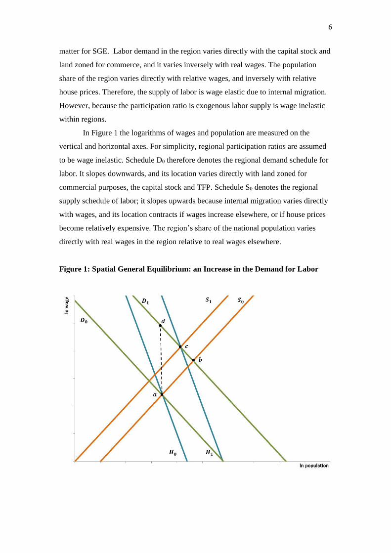
In Figure 1 the logarithms of wages and population are measured on the

vertical and horizontal axes. For simplicity, regional participation ratios are assumed

to be wage inelastic. Schedule D0 therefore denotes the regional demand schedule for

labor. It slopes downwards, and its location varies directly with land zoned for

commercial purposes, the capital stock and TFP. Schedule S0 denotes the regional

supply schedule of labor; it slopes upwards because internal migration varies directly

with wages, and its location contracts if wages increase elsewhere, or if house prices

become relatively expensive. The region’s share of the national population varies

directly with real wages in the region relative to real wages elsewhere.

Figure 1: Spatial General Equilibrium: an Increase in the Demand for Labor

7

Schedule H0 plots the combinations of wages and population that support

regional house prices at PHo. It slopes downwards because the demand for housing

varies directly with wages and population, and is flatter the greater the income

elasticity of demand for housing space. Above schedule H there is an excess demand

for housing, which would raise house prices and which causes schedule H to shift

upwards by an extent which varies inversely with the price elasticity of demand for

housing. Schedule H shifts upwards if land zoned for housing increases, because PHo

is supported by larger combinations of wages and population. Schedule H shifts

downwards if house prices and land zoned for housing increases elsewhere because

builders prefer to construct elsewhere.

Spatial general equilibrium (SGE) occurs at point a in Figure 1, where the

housing market is in equilibrium, and the supply of labor equals the demand for it.

Relative real wages are defined as:

)1(

H

H

P

P

w

wRRW

where bars denote variables elsewhere, and is the share of housing in consumption.

If RRW = 1, real wages adjusted for living costs (house prices) are equated. But there

is no reason why RRW should equal 1 unless labor is perfectly mobile.

An increase in TFP in the region raises the demand for labor to D1. At point b

(intersection between D1 and S0)there is an excess demand for housing. The increase

in house prices shifts schedule H0 to H1 and schedule S0 contracts to S1. The new SGE

is at a point such as c (intersection of schedules D1, H1 and S1).

Notice that at c the population does not necessarily increase relative to a. This

will happen if schedule S contracts by more than schedule H expands when house

prices increase. Nor must schedule H be steeper than schedule D. These slopes are

unrestricted by theory. Indeed, there is an entire taxonomy of SGEs so that the

response of population, wages and house prices to e.g. TFP shocks is indeterminate.

SGE occurs on schedule D1 to the north-east of point b. If SGE occurs on segment db

population, wages and house prices increase. If SGE occurs to the north-east of d

wages and house prices increase, but population decreases. This indeterminacy

increases when the regions are mutually dependent, and when the schedules featured

in Figure 1 are asymmetric. For example, schedule H may be flatter than schedule D

in some regions but steeper in others. The scope for indeterminacy naturally increases

8

with the number of regions. As noted, Brakman, Garretsen and van Marrewijk (2009)

have criticized theory derived for two region models for predicting what happens in N

regions. This criticism holds a fortiori if the regions are asymmetric. In our case N =

9, which naturally increases the potential for spatial state dependence in which the

propagation of shocks in housing, land, and labor markets depends on where they

occur.

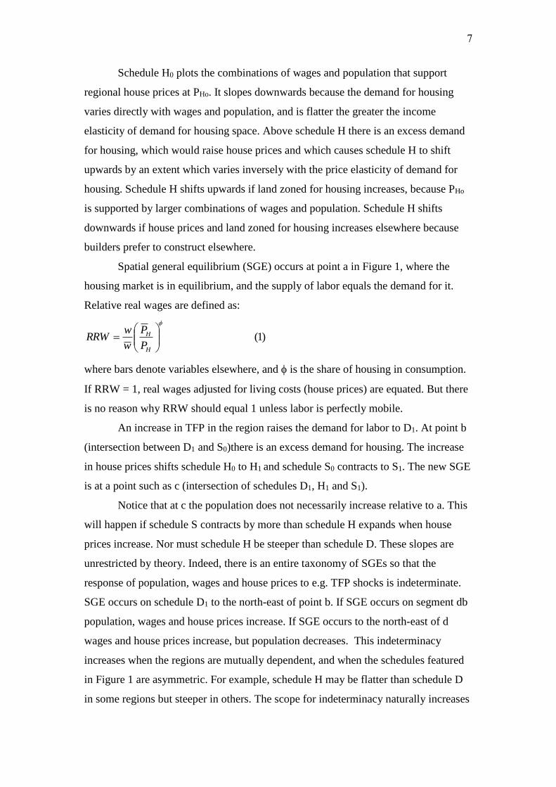
An increase in land zoned for housing would raise schedule H0 to H1 (Figure

2). House prices along schedules H0 and H1 are the same (PH0). At point a there is an

excess supply of housing, which lowers house prices, thereby contracting H1 to H2

and expanding S0 to S1. Schedule S0H1 plots the locus of intersections between

schedules S and H as house prices decrease (below b) or increase (above b). House

prices continue to decrease until the new SGE is reached at point d at which wages

and house prices are lower and population is higher. This result does not depend on

whether schedule D is flatter than schedule H.

Figure 2: Spatial General Equilibrium: an Increase in Land Zoned for Housing

Data

9

We have developed an annual database for nine regions in Israel (see map) during

1987 – 2010. These regions have been selected because house price data have been

published for them since the early 1970s by the Central Bureau of Statistics (CBS). In

the absence of regional income accounts we have constructed annual panel data for

these 9 regions for such variables as housing starts, completions and stocks, wages,

employment, schooling, capital, population etc. Since we have described this database

elsewhere (Beenstock and Felsenstein 2008, 2015) we provide minimal details here.

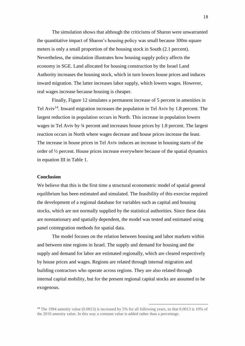
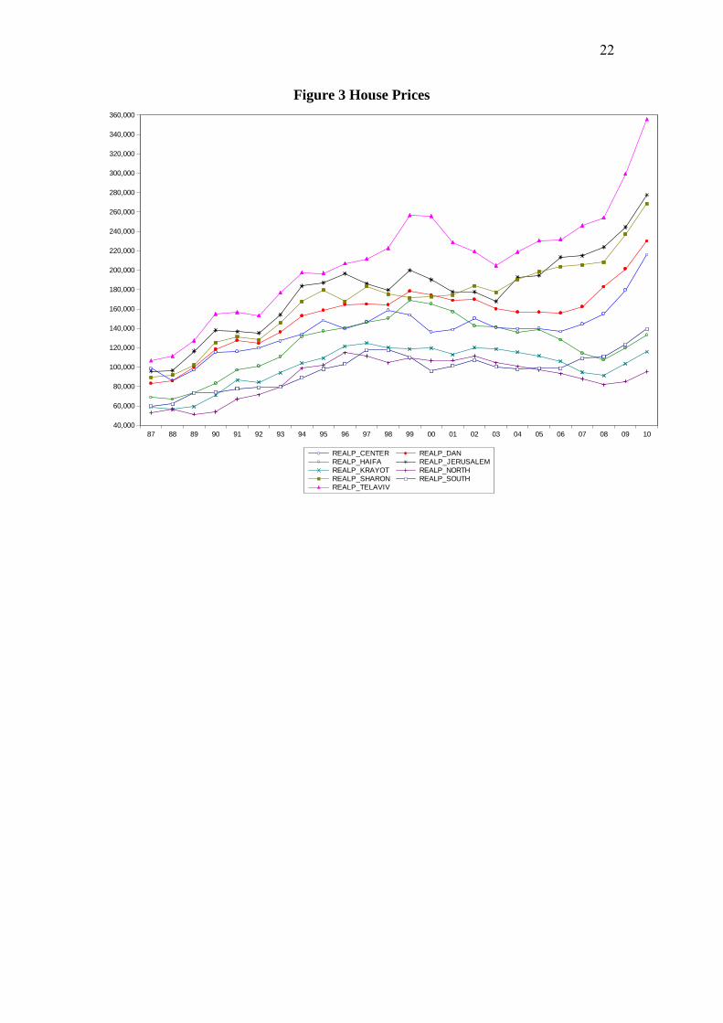
Figures 3 – 8 plot key variables over time and space. Population has risen everywhere

on the background of the arrival of a million immigrants from the former USSR

during the 1990s. Also the natural rate of increase in the national population is

relatively high (about 2% pa). The population increased from 4.5 million in 1987 to 8

million in 2012. Notice that despite the fact that GDP per head grew at an annual rate

of about 1.8% pa, wages did not grow during the 1990s and grew only slowly

subsequently. The last two decades have favored capital at the expense of labor partly

because demographic factors have increased labor supply.

House prices doubled in real terms during the wave of immigration from the

former USSR in the early 1990s. However, Figure 3 shows that the increase in house

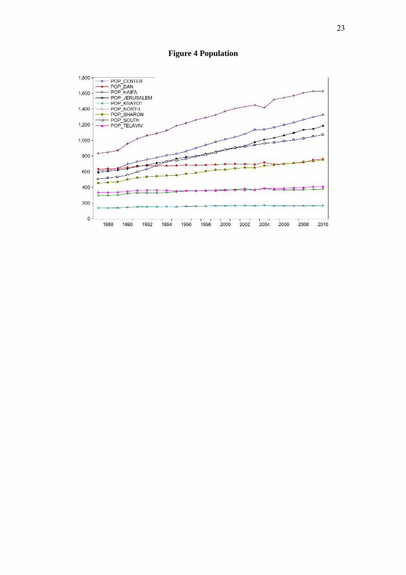
prices was not uniform. The same applies to population (Figure 4). Figure 5 shows

that with the exception of the early 1990s when the wave of immigration crested,

housing construction kept pace with the rate of population growth so that housing

space per capita increased. However, there is substantial regional variation in this

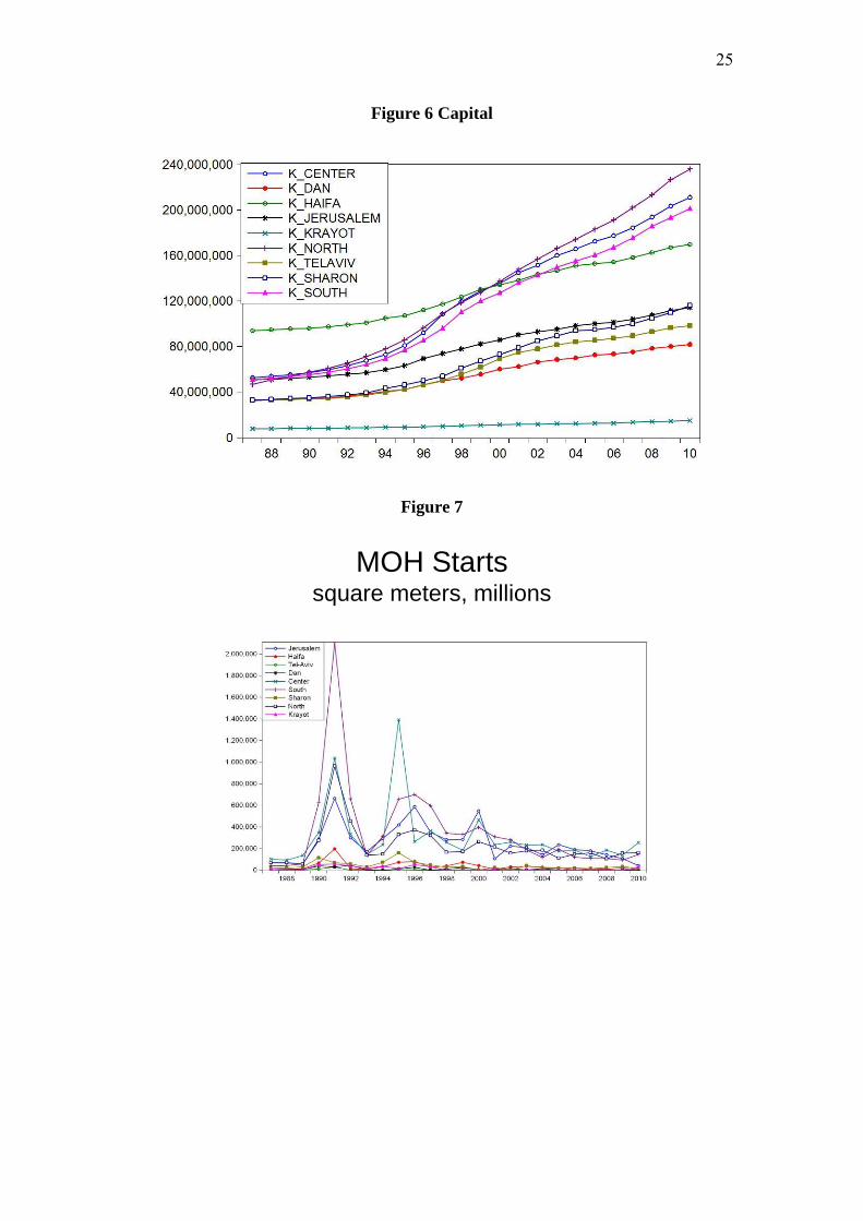
measure of housing density. Finally, Figure 6 plots capital stocks; it shows that capital

grew more slowly in capital abundant regions, such as North, and more rapidly in

capital scarce regions, thereby inducing beta and sigma convergence in capital stocks.

The Israel Land Authority (ILA) is a unique institution in which

approximately 90 percent of land in Israel is vested. The balance is owned privately6.

ILA auctions land for housing construction (and commercial purposes) to building

contractors, who sell completed housing in the private market to the public. Home-

owners are given 50-year leaseholds with ILA, which are renewable at zero cost. The

main purpose of ILA is political; to give the government ultimate control over land

ownership. ILA is highly politicized. It is currently answerable to the Minister of

Housing and Construction (MOHC), and land for housing construction is frequently

6 Mainly by churches and freeholds dating back to Ottoman rule which ended in 1918.

10

made available by ILA on a partisan basis. We estimate that ILA currently holds

enormous land reserves for housing equal to all the built-up land in Israel.

Unfortunately, these reserves are in locations where residential demand is low. Figure

6 plots land auctioned for residential purposes by ILA7. It shows that land for housing

has been sold-off mainly in the periphery. These land sales constitute a major

instrument of regional policy, and play a central role in the econometric model for

identifying housing supply.

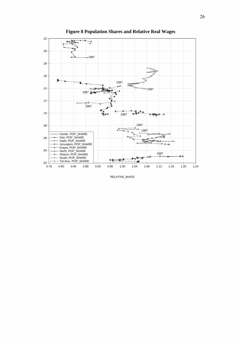
Figure 8 plots population shares against relative real wages (RRW) for each

of the nine regions. The data points are joined chronologically so that the first point

refers to 1987 and the last to 2010. The population shares in Center, Dan and Krayot

vary directly with relative real wages, as expected. Over the entire period South’s

population share and its relative real wage increased, however, the latter preceded the

former. In two regions, North and Haifa, population shares increased but relative real

wages zig-zagged without increasing. In Sharon relative real wages increased but its

population share did not change. Finally, in Tel Aviv and Jerusalem the relationship

between population shares and relative real wages slopes the “wrong” way. In Tel

Aviv relative real wages increased but its population share decreased. The opposite

happened in Jerusalem; relative real wages decreased but its population share

increased.

Panel Cointegration

In spatial panel data unit roots that induce nonstationarity in the data may arise from

either or both of two reasons. There may be temporal unit roots that arise in nonspatial

data, and there may be spatial unit roots (Yu, de Jong and Lee 2012, Beenstock and

Felsenstein 2012) induced by unit eigenvalues in W or by unit SAR coefficients. We

have established elsewhere that our panel data are nonstationary for the former

reason. Since parameter estimates may be spurious in nonstationary panel data

(Phillips and Moon 1999) we use panel cointegration tests due to Pedroni (1999,

2004). Specifically we use the grouped ADF statistic (GADF) for the residuals.

Pedroni’s critical values assume that cross-section units are independent. Banerjee

and Carrion-I-Silvestre (2011) have calculated critical values for strong cross-section

dependence and Beenstock and Felsenstein (2015) show that Pedroni’s critical values

7 In CBS publications these data are referred to as “housing starts under public initiative”.

11

are salient for weak (spatial) cross-section dependence for SAR coefficients less than

0.4. These critical values are indicative only because they have not as yet been

calculated for cointegration in spatial panel data models. For example, Banerjee and

Carrion-I-Silvestre report that the critical value of GADF at p = 0.05 is -2.57 when N

= 10, T = 20 and there are three cointegrating variables. The model is cointegrated

and the results are not spurious if the estimated residuals are stationary, i.e. GADF is

smaller than its critical value 8.

Because the structural equations of the model are estimated using panel

cointegration, the model refers to long-term relations between the state variables. We

do not estimate the error correction models associated with these cointegrating

relations because economic theory is more restrictive about long-term behavior than

about short-term behavior. Therefore, the model ignores short-term dynamics. More

generally, it ignores stationary components of the state variables such as the role of

expectations (especially of house prices and inflation) and partial adjustment

mechanisms (especially in wage determination and housing construction).

The equations in the model have the following generic spatial Durbin

specification:

tttt

ttttt

WYYWXX

uYXXY

~~

)2(~~

where Y, X and u are column vectors of length N, is an N-vector of fixed regional

effects, tildes denote spatially lagged variables, and W is an NxN spatial connectivity

matrix row-summed to one, with zeros along the leading diagonal, and with

eigenvalues less than 1. Since Y and X are difference stationary, so are spatial lagged

variables difference stationary because W does not generally constitute a matrix of

cointegrating vectors. Panel cointegration requires that u be stationary9. If u is

stationary when = = 0, equation (2) is “locally cointegrated” because cointegration

is induced within spatial units. If u is stationary when = 0, equation (2) is “spatially

cointegrated” because cointegration is induced between spatial units. If none of these

8 We do not use estimators for spatial cointegration proposed e.g. by Yu, de Jong and Lee (2012)

because the unit roots in the data are temporal rather than spatial. 9 The 1st order error correction model associated with equation (2) is

ttttttt XfYeXdYcbuaY 11111

~~

where b < 0 is the error correction coefficient and is iid. As mentioned, we do not estimate error

correction models.

12

restrictions apply, then equation (2) is “generally cointegrated” because cointegration

is induced within and between spatial units10.

The solution for Yt from equation (2) is:

)()(

)3()(

1 WiABWIA

BXuAY

NN

ttt

in which case the spatial propagation of X in region j on Y in region i is bij = aij + cij

where C = AW. The counterpart for innovations is aij.

In cointegrated time series models the parameter estimates are super-

consistent (Stock 1987) in which case potential reverse causality from Y to X in

equation (2) would not affect the consistency of , although it may be biased in finite

samples (Banerjee et al 1993). Matters are different in nonstationary panel data

because the bias induced by cross-section dependence between state variables does

not tend to zero with N (Phillips and Moon 1999). However, if N is fixed as it is in

spatial panel data, it may be shown that this bias tends to zero with T (Beenstock and

Felsenstein 2015). This means that model covariates, such as X in equation (2) are

weakly exogenous11, in which case the parameter estimates are consistent.

Similar reasoning applies to , which in stationary panel data must be

estimated by maximum likelihood (Elhorst 2003) since dependent variables and

spatial lagged dependent variables are jointly determined. In nonstationary panel data

OLS estimates of SAR coefficients are consistent (Beenstock and Felsenstein 2015)

provided the model is panel cointegrated; because Y~

~ I(1) and u ~ I(0) are

asymptotically independent.

We do not report equation standard errors because estimates of cointegrating

vectors generally have non-standard distributions. Instead, tests of parameter

restrictions are carried out by imposing the restrictions and using the cointegration test

statistic to evaluate them. For example, if the model ceases to be cointegrated when a

restriction is imposed, the restriction is rejected. If, however, the p-value for

cointegration does not depend on the restriction, the restriction is accepted.

10 Notice that Y and Y

~and X and X

~are not generally cointegrated with each other.

11 Since the covariates are integrated to order 1 and the residuals are integrated to order zero, there can

be no asymptotic relation between the covariates and the residuals. In spatial panel data super-

consistency depends on the number of time series observations (T) not the number of cross-section

observations (N).

13

The spatial weighting scheme is given by equation VIII in Table 1. It varies

inversely with distance (d) and it is asymmetric unless the average populations of i

and j happen to be the same12. Therefore, bigger neighbors have a greater spatial

weight than smaller neighbors. Agglomeration (A) at the beginning of period t is

defined in equation IX. It varies directly with “capital experience” as measured by the

capital-labor ratio (k) in period t-1, and it depreciates by 5 percent per year. The time

series properties of A are therefore the same as those of k. Using capital creates new

knowledge through learning-by-going, which increases TFP.

The Model

The empirical model described in this section is based on the theoretical model

described in section 2, but in bringing theory to data a number of extensions are

required. First, there are nine dependent regions rather than only one “small” region.

However, each region may be characterized as in Figure 1; there are supply and

demand schedules for housing and labor. Second, whereas the theoretical model did

not articulate the gestation lag in housing construction, the empirical model specifies

the dynamic relation between housing starts and completions. Because the housing

stock is quasi-fixed in the short-run but variable thereafter the empirical model

distinguishes between temporary and permanent (steady state) equilibria Third, the

Israel Land Authority, which was ignored in the theoretical model plays a central role

in the empirical model as the source of land zoned for housing construction. Fourth,

amenities which had no role in the theoretical model are specified in the empirical

model.

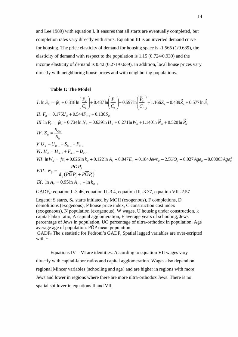
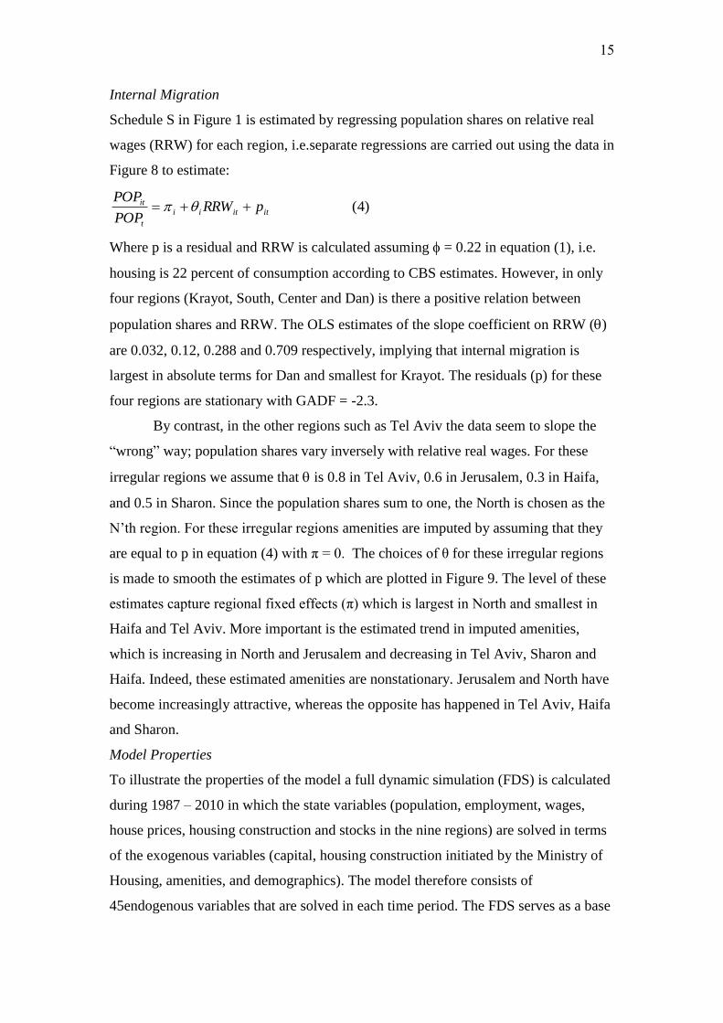
The main equations of the model are reported in Table 1. Housing starts (S)

are determined by Equation I according to which starts vary directly with house prices

(P) and construction incentives provided by the Ministry of Housing and Construction

(Z), inversely with building costs (C), as well as spatial lags of these variables13.

These spatial lag coefficients are negative because there is spatial substitution in

housing construction. The spatial lagged dependent variable is positive (0.557) due to

spatial spillover in housing construction. The overall price elasticity of housing starts

is 0.28. Equation II relates completions to starts and is multi-cointegrated (Granger

12 Note that W does not depend on t because it refers to the sample average. 13 See Beenstock and Felsenstein (2015) for details and further explanations for equations I, II, V and

V1.

14

and Lee 1989) with equation I. It ensures that all starts are eventually completed, but

completion rates vary directly with starts. Equation III is an inverted demand curve

for housing. The price elasticity of demand for housing space is -1.565 (1/0.639), the

elasticity of demand with respect to the population is 1.15 (0.724/0.939) and the

income elasticity of demand is 0.42 (0.271/0.639). In addition, local house prices vary

directly with neighboring house prices and with neighboring populations.

Table 1: The Model

2

111

111

1

00063.0027.05.2184.0047.0ln122.0ln026.0ln.

.

.

~ln520.0

~ln140.1ln271.0ln639.0ln734.0ln

136.0544.0175.0.

~ln577.0

~439.0166.1

~

ln597.0ln487.0ln318.0ln.

itititititititiit

itititit

itititit

it

Gitit

itititititiit

itititit

ttt

t

it

t

t

t

itiit

AgeAgeUOJewsEAkfeWVII

DFHHVI

FSUUV

S

SZIV

PNWHNfePIII

SFUFII

SZZC

P

C

P

C

PfeSI

11 lnln95.0ln.

)(.

ititit

ijij

j

ij

kAAIX

POPPOPd

POPwVIII

GADFz: equation I -3.46, equation II -3.4, equation III -3.37, equation VII -2.57

Legend: S starts, SG starts initiated by MOH (exogenous), F completions, D

demolitions (exogenous), P house price index, C construction cost index

(exogeneous), N population (exogenous), W wages, U housing under construction, k

capital-labor ratio, A capital agglomeration, E average years of schooling, Jews

percentage of Jews in population, UO percentage of ultra-orthodox in population, Age

average age of population. PŌP mean population.

GADFz The z statistic for Pedroni’s GADF, Spatial lagged variables are over-scripted

with ~.

Equations IV – VI are identities. According to equation VII wages vary

directly with capital-labor ratios and capital agglomeration. Wages also depend on

regional Mincer variables (schooling and age) and are higher in regions with more

Jews and lower in regions where there are more ultra-orthodox Jews. There is no

spatial spillover in equations II and VII.

15

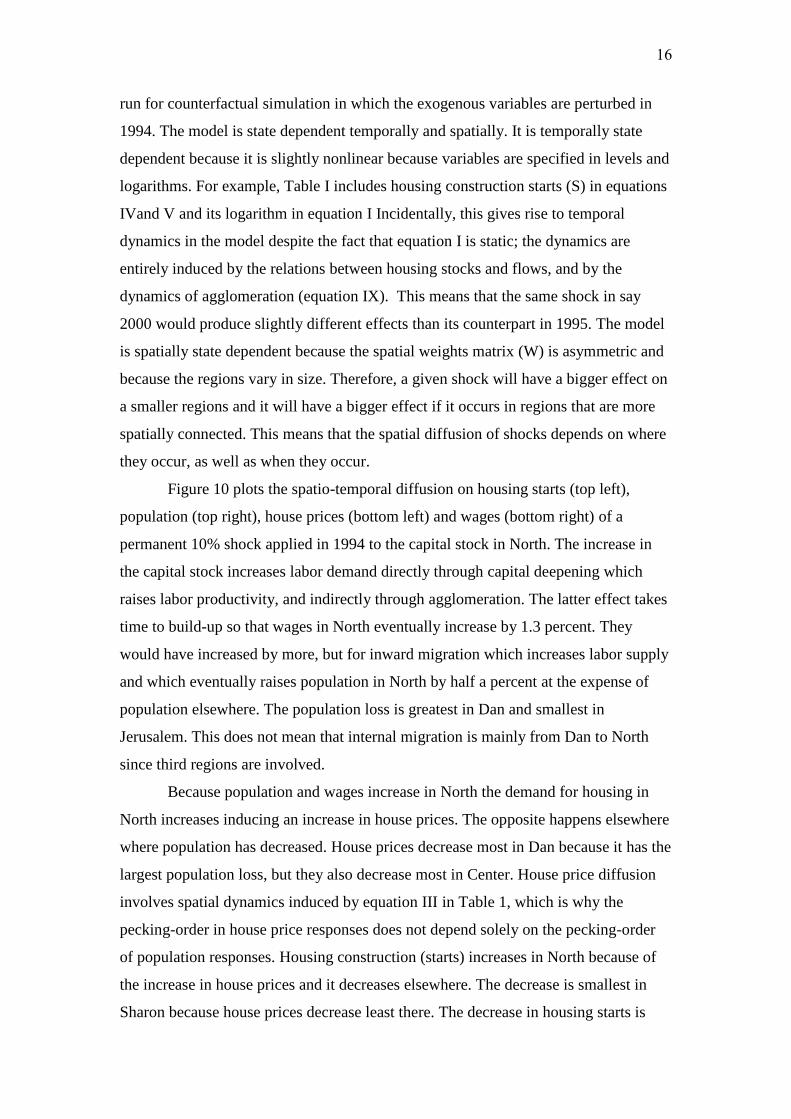
Internal Migration

Schedule S in Figure 1 is estimated by regressing population shares on relative real

wages (RRW) for each region, i.e.separate regressions are carried out using the data in

Figure 8 to estimate:

)4(ititii

t

it pRRWPOP

POP

Where p is a residual and RRW is calculated assuming = 0.22 in equation (1), i.e.

housing is 22 percent of consumption according to CBS estimates. However, in only

four regions (Krayot, South, Center and Dan) is there a positive relation between

population shares and RRW. The OLS estimates of the slope coefficient on RRW ()

are 0.032, 0.12, 0.288 and 0.709 respectively, implying that internal migration is

largest in absolute terms for Dan and smallest for Krayot. The residuals (p) for these

four regions are stationary with GADF = -2.3.

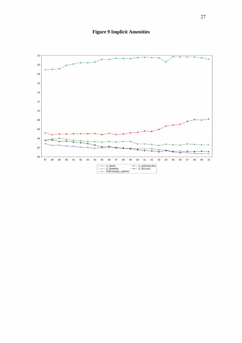
By contrast, in the other regions such as Tel Aviv the data seem to slope the

“wrong” way; population shares vary inversely with relative real wages. For these

irregular regions we assume that is 0.8 in Tel Aviv, 0.6 in Jerusalem, 0.3 in Haifa,

and 0.5 in Sharon. Since the population shares sum to one, the North is chosen as the

N’th region. For these irregular regions amenities are imputed by assuming that they

are equal to p in equation (4) with π = 0. The choices of θ for these irregular regions

is made to smooth the estimates of p which are plotted in Figure 9. The level of these

estimates capture regional fixed effects (π) which is largest in North and smallest in

Haifa and Tel Aviv. More important is the estimated trend in imputed amenities,

which is increasing in North and Jerusalem and decreasing in Tel Aviv, Sharon and

Haifa. Indeed, these estimated amenities are nonstationary. Jerusalem and North have

become increasingly attractive, whereas the opposite has happened in Tel Aviv, Haifa

and Sharon.

Model Properties

To illustrate the properties of the model a full dynamic simulation (FDS) is calculated

during 1987 – 2010 in which the state variables (population, employment, wages,

house prices, housing construction and stocks in the nine regions) are solved in terms

of the exogenous variables (capital, housing construction initiated by the Ministry of

Housing, amenities, and demographics). The model therefore consists of

45endogenous variables that are solved in each time period. The FDS serves as a base

16

run for counterfactual simulation in which the exogenous variables are perturbed in

1994. The model is state dependent temporally and spatially. It is temporally state

dependent because it is slightly nonlinear because variables are specified in levels and

logarithms. For example, Table I includes housing construction starts (S) in equations

IVand V and its logarithm in equation I Incidentally, this gives rise to temporal

dynamics in the model despite the fact that equation I is static; the dynamics are

entirely induced by the relations between housing stocks and flows, and by the

dynamics of agglomeration (equation IX). This means that the same shock in say

2000 would produce slightly different effects than its counterpart in 1995. The model

is spatially state dependent because the spatial weights matrix (W) is asymmetric and

because the regions vary in size. Therefore, a given shock will have a bigger effect on

a smaller regions and it will have a bigger effect if it occurs in regions that are more

spatially connected. This means that the spatial diffusion of shocks depends on where

they occur, as well as when they occur.

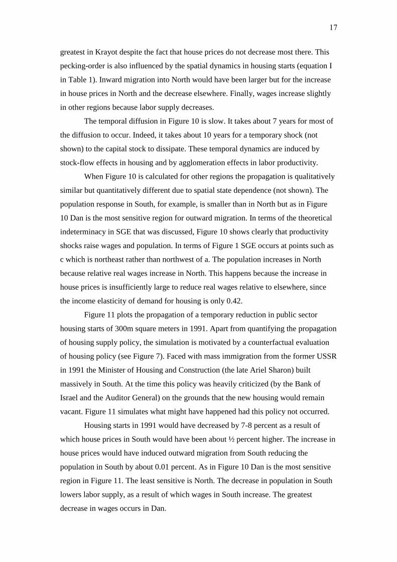
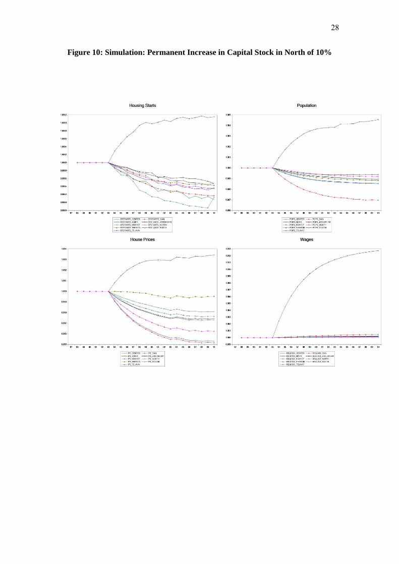
Figure 10 plots the spatio-temporal diffusion on housing starts (top left),

population (top right), house prices (bottom left) and wages (bottom right) of a

permanent 10% shock applied in 1994 to the capital stock in North. The increase in

the capital stock increases labor demand directly through capital deepening which

raises labor productivity, and indirectly through agglomeration. The latter effect takes

time to build-up so that wages in North eventually increase by 1.3 percent. They

would have increased by more, but for inward migration which increases labor supply

and which eventually raises population in North by half a percent at the expense of

population elsewhere. The population loss is greatest in Dan and smallest in

Jerusalem. This does not mean that internal migration is mainly from Dan to North

since third regions are involved.

Because population and wages increase in North the demand for housing in

North increases inducing an increase in house prices. The opposite happens elsewhere

where population has decreased. House prices decrease most in Dan because it has the

largest population loss, but they also decrease most in Center. House price diffusion

involves spatial dynamics induced by equation III in Table 1, which is why the

pecking-order in house price responses does not depend solely on the pecking-order

of population responses. Housing construction (starts) increases in North because of

the increase in house prices and it decreases elsewhere. The decrease is smallest in

Sharon because house prices decrease least there. The decrease in housing starts is

17

greatest in Krayot despite the fact that house prices do not decrease most there. This

pecking-order is also influenced by the spatial dynamics in housing starts (equation I

in Table 1). Inward migration into North would have been larger but for the increase

in house prices in North and the decrease elsewhere. Finally, wages increase slightly

in other regions because labor supply decreases.

The temporal diffusion in Figure 10 is slow. It takes about 7 years for most of

the diffusion to occur. Indeed, it takes about 10 years for a temporary shock (not

shown) to the capital stock to dissipate. These temporal dynamics are induced by

stock-flow effects in housing and by agglomeration effects in labor productivity.

When Figure 10 is calculated for other regions the propagation is qualitatively

similar but quantitatively different due to spatial state dependence (not shown). The

population response in South, for example, is smaller than in North but as in Figure

10 Dan is the most sensitive region for outward migration. In terms of the theoretical

indeterminacy in SGE that was discussed, Figure 10 shows clearly that productivity

shocks raise wages and population. In terms of Figure 1 SGE occurs at points such as

c which is northeast rather than northwest of a. The population increases in North

because relative real wages increase in North. This happens because the increase in

house prices is insufficiently large to reduce real wages relative to elsewhere, since

the income elasticity of demand for housing is only 0.42.

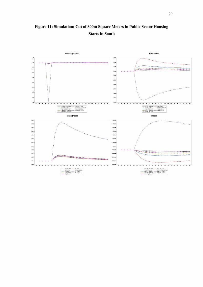
Figure 11 plots the propagation of a temporary reduction in public sector

housing starts of 300m square meters in 1991. Apart from quantifying the propagation

of housing supply policy, the simulation is motivated by a counterfactual evaluation

of housing policy (see Figure 7). Faced with mass immigration from the former USSR

in 1991 the Minister of Housing and Construction (the late Ariel Sharon) built

massively in South. At the time this policy was heavily criticized (by the Bank of

Israel and the Auditor General) on the grounds that the new housing would remain

vacant. Figure 11 simulates what might have happened had this policy not occurred.

Housing starts in 1991 would have decreased by 7-8 percent as a result of

which house prices in South would have been about ½ percent higher. The increase in

house prices would have induced outward migration from South reducing the

population in South by about 0.01 percent. As in Figure 10 Dan is the most sensitive

region in Figure 11. The least sensitive is North. The decrease in population in South

lowers labor supply, as a result of which wages in South increase. The greatest

decrease in wages occurs in Dan.

18

The simulation shows that although the criticisms of Sharon were unwarranted

the quantitative impact of Sharon’s housing policy was small because 300m square

meters is only a small proportion of the housing stock in South (2.1 percent).

Nevertheless, the simulation illustrates how housing supply policy affects the

economy in SGE. Land allocated for housing construction by the Israel Land

Authority increases the housing stock, which in turn lowers house prices and induces

inward migration. The latter increases labor supply, which lowers wages. However,

real wages increase because housing is cheaper.

Finally, Figure 12 simulates a permanent increase of 5 percent in amenities in

Tel Aviv14. Inward migration increases the population in Tel Aviv by 1.8 percent. The

largest reduction in population occurs in North. This increase in population lowers

wages in Tel Aviv by ¾ percent and increases house prices by 1.8 percent. The largest

reaction occurs in North where wages decrease and house prices increase the least.

The increase in house prices in Tel Aviv induces an increase in housing starts of the

order of ½ percent. House prices increase everywhere because of the spatial dynamics

in equation III in Table 1.

Conclusion

We believe that this is the first time a structural econometric model of spatial general

equilibrium has been estimated and simulated. The feasibility of this exercise required

the development of a regional database for variables such as capital and housing

stocks, which are not normally supplied by the statistical authorities. Since these data

are nonstationary and spatially dependent, the model was tested and estimated using

panel cointegration methods for spatial data.

The model focuses on the relation between housing and labor markets within

and between nine regions in Israel. The supply and demand for housing and the

supply and demand for labor are estimated regionally, which are cleared respectively

by house prices and wages. Regions are related through internal migration and

building contractors who operate across regions. They are also related through

internal capital mobility, but for the present regional capital stocks are assumed to be

exogenous.

14 The 1994 amenity value (0.0013) is increased by 5% for all following years, so that 0.0013 is 10% of

the 2010 amenity value. In this way a constant value is added rather than a percentage.

19

In Israel the government has two policy instruments for influencing the spatial

distribution of economic activity, the zoning of land for housing construction and

commercial purposes, and investment grants and subsidies differentiated by region.

The model is used to simulate these polices. For example, increasing land zoned for

housing increases housing construction and lowers house prices, which increases

labor supply through internal migration. The latter decreases wages and increases the

demand for housing. Investment grants which increase capital investment increase

labor productivity and wages which induce inward migration. House prices increase

because housing demand varies directly with population and income. Housing

construction increases because construction is more profitable, which moderates the

initial increase in house prices.

These policy instruments are place-based rather than people-based. Glaeser

and Gottlieb (2008) think that labor and capital are sufficiently internally mobile to

guarantee that spatial factor price equalization occurs within a sufficiently short

period of time. Accordingly, they think that place-based policies are redundant, and

that people-based polices should be applied to encourage internal mobility. By

contrast, Partridge et al (2013) think that placed-based policies are justified on second

best grounds. Our results are relevant to this debate in three respects. First, the forces

of internal migration are insufficiently strong to eliminate regional wage inequality

even in the long-term. Second, regional shocks in housing, labor and capital markets

are slow to dissipate; they persist even after 10-15 years. Third, agglomeration

aggravates this persistence and induces regional divergence rather than convergence.

These results suggest a prima facie case for place-based policy. If places matter to the

public and to building contractors in a small and young country such as Israel where

regional allegiances and cultures are not yet fully developed, they are likely to matter

even more in larger and more mature countries.

In the case of Israel, it can be argued that the place-based versus people-based

policies dichotomy may be exaggerated. This is because 90 percent of land and almost

half of land reserves are vested in the Israel Land Authority. This dominance means

that any place-based policy is also inherently people-based. Divestment of these land

reserves for housing and commercial purposes inevitably has implications for places

as well as people. Since these land reserves are concentrated in the periphery of the

country, a regional shock in the form of divestment would benefit the peripheral

20

regions and attract people and investment away from the congested center of the

country.

21

Map

22

Figure 3 House Prices

40,000

60,000

80,000

100,000

120,000

140,000

160,000

180,000

200,000

220,000

240,000

260,000

280,000

300,000

320,000

340,000

360,000

87 88 89 90 91 92 93 94 95 96 97 98 99 00 01 02 03 04 05 06 07 08 09 10

REALP_CENTER REALP_DAN

REALP_HAIFA REALP_JERUSALEM

REALP_KRAYOT REALP_NORTH

REALP_SHARON REALP_SOUTH

REALP_TELAVIV

23

Figure 4 Population

24

Figure 5 Housing Space per Head

25

Figure 6 Capital

Figure 7

MOH Startssquare meters, millions

26

Figure 8 Population Shares and Relative Real Wages

.02

.04

.06

.08

.10

.12

.14

.16

.18

.20

.22

0.76 0.80 0.84 0.88 0.92 0.96 1.00 1.04 1.08 1.12 1.16 1.20 1.24

RELATIVE_WAGE

Center, POP_SHARE

Dan, POP_SHARE

Haifa, POP_SHARE

Jerusalem, POP_SHARE

Krayot, POP_SHARE

North, POP_SHARE

Sharon, POP_SHARE

South, POP_SHARE

Tel-Aviv, POP_SHARE

1987

1987

1987

1987

1987

1987

1987

1987

1987

27

Figure 9 Implicit Amenities

.00

.02

.04

.06

.08

.10

.12

.14

.16

.18

.20

.22

87 88 89 90 91 92 93 94 95 96 97 98 99 00 01 02 03 04 05 06 07 08 09 10

A_HAIFA A_JERUSALEM

A_SHARON A_TELAVIV

POPSHARE_NORTH

28

Figure 10: Simulation: Permanent Increase in Capital Stock in North of 10%

29

Figure 11: Simulation: Cut of 300m Square Meters in Public Sector Housing

Starts in South

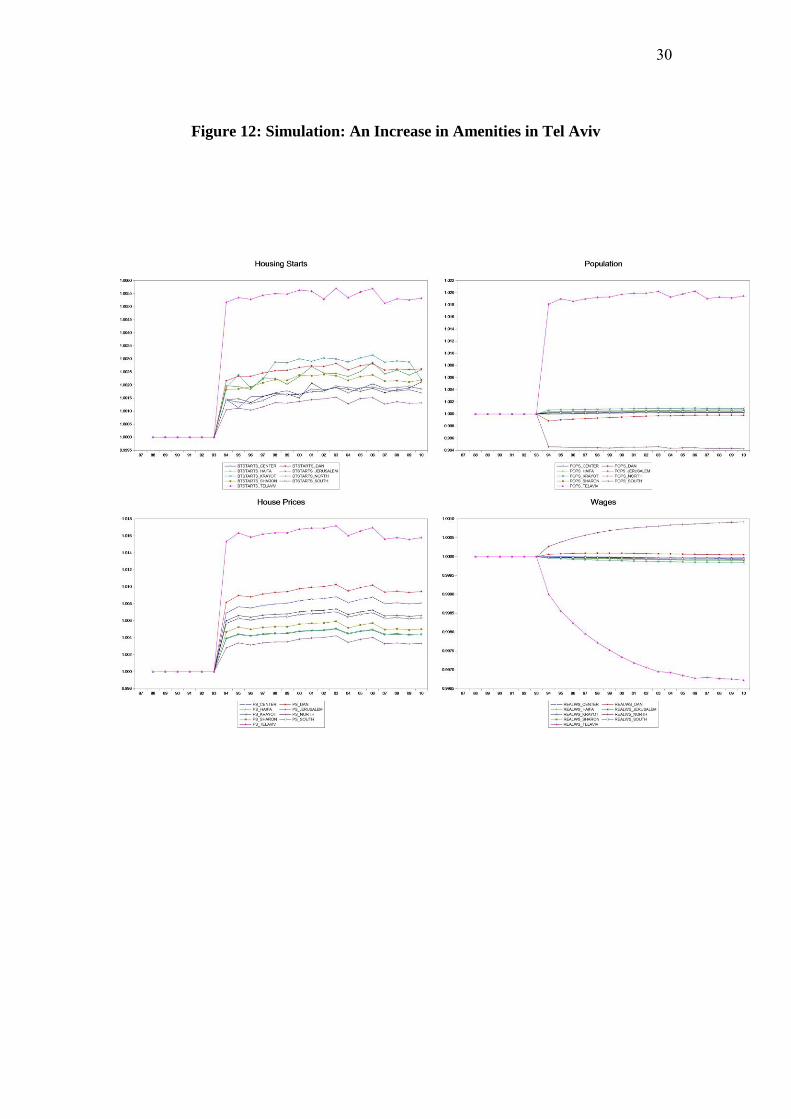
30

Figure 12: Simulation: An Increase in Amenities in Tel Aviv

31

References

Baldwin R.E and Martin P. (2004) Agglomeration and Regional Growth, pp 2672-

2711 in Vernon Henderson J and Thisse J-F (eds) Handbook of Regional and Urban

Economics Vol 4, Elsevier, Holland

Banerjee A., J. Dolado, J.W. Galbraith and D.F. Hendry (1993) Cointegration,Error

Correction, and the Econometric Analysis of Nonstationary Time Series. Oxford

University Press.

Banerjee A and Carrion-I-Silvestre J.L (2011) Testing for panel cointegration using

common correlated effects estimators. Dept of Economics, University of

Birmingham.

Beenstock M. and D. Felsenstein (2010) Spatial error correction and cointegration in

nonstationary spatial panel data: regional house prices in Israel. Journal of

Geographical Systems, 12: 189-206.

Beenstock M. and D. Felsenstein (2010) Marshallian theory of regional

agglomeration. Papers in Regional Science, 89: 155-172.

Beenstock M. and D. Felsenstein (2015) Spatial spillover in housing supply. Journal

of Housing Economics, 28, 42-53

Beenstock M., D. Felsenstein and N. Ben Zeev (2011) Capital deepening and regional

inequality: an empirical analysis. Annals of Regional Science, 47: 599-617.

Beenstock M., D. Feldman and D. Felsenstein (2012) Testing for Units Roots

and Cointegration in Spatial Cross Section Data, Spatial Economic Analysis

7(2), 203-222.

Beenstock M., D. Felsenstein and D. Xieer (2015) Spatial econometric analysis of

regional housing markets. Mimeo.

Brandsma, A, Kancs d’A, Monfort P and Rillaers A (2013) RHOMLO: A Dynamic

Spatial General Equilibrium Model for Assessing the Impact of Cohesion Policy,

EUR 25957 – Joint Research Centre – Institute for Prospective Technological Studies,

Publications Office of the European Union, Luxembourg.

Brakman S and Garretsen H (2006) New Economic Geography: Closing the Gap

between Theory and Empirics, Regional Science and Urban Economics, 36, 569-572.

Brakman S., H. Garretson and C. van Marrewijk (2009) The New Introduction to

Geographical Economics, 2nd edition, Cambridge University Press.

32

Buchinsky M., Gotlibovski C and Lifshitz O. (2014) Residential Location, Work

Location, and Labor Market Outcomes of Immigrants in Israel, Econometrica,82

(3), 995-1054.

Combes P-P., T. Mayer and J-F. Thisse (2008) Economic Geography: the Integration

of Regions and Nations, Princeton University Press.

Davis D.R. and D. Weinstein (2003) Market access, economic geography and

comparative advantage: an empirical assessment. Journal of International Economics,

59: 1-23.

Elhorst J.P (2003) Specification and estimation of spatial panel data models.

International Journal of Regional Science, 25: 244-268.

Giesecke J.A and Madden J.R. (2013) Regional computable general

equilibrium modeling pp 377-475 in Dixon P.B and Jorgensen D.W (eds) Handbook

of Computable General Equilibrium Modeling, Vol 1, Elsevier Holland.

Johnes G and Hyclak T (1999) House prices and regional labor markets, Annals of

Regional Science, 33, 33-49

Glaeser E. L., Kalko J. and Saiz A. (2001), Consumer City, Journal of Economic

Geography, 1, 27-50.

Glaeser E.L. and Gottlieb J.D (2008) The Economics of place-making policies,

Brookings Papers on Economic Activity, 1,: 155–239.

Glaeser E.L. and J.D. Gottlieb (2009) The wealth of cities: agglomeration economies

and spatial equilibrium in the United States. Journal of Economic Literature, 47: 983-

1028.

Granger, C.W.J., Lee, T., (1989) Investigation of production, sales and inventory

relations using multi-cointegration and non-symmetric error correction models.

Journal of Applied Econometrics, 4, S145-S159.

Greenwood M.U. and R. Stock (1990) Patterns of change in the intrametropolitan

location of population, jobs and housing. Journal of Urban Economics, 28: 243-276.

Hanson G. (2005) Market potential, increasing returns, and geographic concentration.

Journal of International Economics, 67: 1-24.

Head K and T. Mayer (2004) Market potential and the location of Japanese

investment in the European Union. Review of Economics and Statistics, 86: 959-972.

Krugman P. (1991) Geography and Trade. MIT Press.

Partridge M.D. and Rickman D.S. (1998) Regional computable general equilibrium

modeling: a survey and critical appraisal, International Regional Science Review,21,

205-248.

33

Partridge M.D.,Rickman D.S.,Rose Olfert M and Tan Y (2013) When spatial

equilibrium fails: is place-based policy second best?, Regional Studies,

http://dx.doi.org/10.1080/00343404.2013.837999

Pedroni P. (2004) Panel cointegration: asymptotic and finite sample properties of

pooled time series tests with an application to the PPP hypothesis, Econometric

Theory, 20: 597-625.

Phillips P.C.B. and H. Moon (1999) Linear regression limit theory for nonstationary

panel data, Econometrica, 67: 1057-1011.

Roback J. (1982) Wages, rents and the quality of life. Journal of Political Economy,

90: 1257-1278.

Stock J. H. (1987) Asymptotic properties of least squares estimators of cointegrating

vectors. Econometrica, 55, 1035-1056.

Vermeulen W and van Ommeren J (2009) Does land use planning shape regional

economies? A simultaneous analysis of housing supply, internal migration and local

employment growth in the Netherlands, Journal of Housing Economics 18, 294–310

Westerlund J. (2007) Error correction based panel cointegration tests, Oxford Bulletin

of Economics and Statistics

Yu J.,R. de Jong and L. Lee (2012) Estimation of spatial dynamic models with fixed

effects: the case of spatial cointegration. Journal of Econometrics, 167: 16-37.