A STEPWISE REGRESSION METHOD AND CONSISTENT...

Submitted to the Annals of StatisticsarXiv: math.PR/0000000

A STEPWISE REGRESSION METHOD AND CONSISTENT MODELSELECTION FOR HIGH-DIMENSIONAL SPARSE LINEAR MODELS

BY CHING-KANG ING ∗ AND TZE LEUNG LAI †

Academia Sinica and Stanford University

We introduce a fast stepwise regression method, called the orthogonalgreedy algorithm (OGA), that selects input variables to enter a p-dimensionallinear regression model (with p >> n, the sample size) sequentially so thatthe selected variable at each step minimizes the residual sum squares. Wederive the convergence rate of OGA as m = mn becomes infinite, and alsodevelop a consistent model selection procedure along the OGA path so thatthe resultant regression estimate has the oracle property of being equivalentto least squares regression on an asymptotically minimal set of relevant re-gressors under a strong sparsity condition.

1. Introduction. Consider the linear regression model

yt = α+p∑j=1

βjxtj + εt, t = 1, 2, · · · , n,(1.1)

with p predictor variables xt1, xt2, · · · , xtp that are uncorrelated with the mean-zero random disturbances εt. When p is larger than n, there are computational andstatistical difficulties in estimating the regression coefficients by standard regres-sion methods. Major advances to resolve these difficulties have been made in thepast decade with the introduction of L2-boosting [2], [3], [14], LARS [11], andLasso [22] which has an extensive literature because much recent attention has fo-cused on its underlying principle, namely, l1-penalized least squares. It has alsobeen shown that consistent estimation of the regression function

y(x) = α+ β>x, where β = (β1, · · · , βp)>,x = (x1, · · · , xp)>,(1.2)

is still possible under a sparseness condition on the regression coefficients. In par-ticular, by assuming the ”weak sparsity” condition that the regression coefficientsare absolutely summable, Buhlmann [2] showed that for p = exp(O(nξ)) with0 < ξ < 1, the conditional mean squared prediction error

CPE := E(y(x)− ym(x))2|y1,x1, · · · , yn,xn(1.3)∗Research supported by the National Science Council, Taiwan, ROC†Research supported by the National Science FoundationAMS 2000 subject classifications: Primary 62J05, 62J99; secondary 60F10, 41A25Keywords and phrases: Componentwise linear regression, Exponential inequality, Greedy algo-

rithm, High-dimensional information criterion, Lasso, Oracle inequality, Sparsity

1

2

of the L2-boosting predictor ym(x) (defined in Section 2.1) can converge in prob-ability to 0 if m = mn → ∞ sufficiently slowly. Fan and Lv [12] recently in-troduced another method, called sure independence screening (SIS), to screen outvariables from high-dimensional regression models, and showed that the proba-bility of including all relevant regressors by using SIS approaches 1 as the sam-ple size becomes infinite. The most comprehensive theory to date for these high-dimensional regression methods has been developed for Lasso and a closely relatedmethod, the Dantzig selector, introduced by Candes and Tao [5]. In particular, or-acle inequalities for the Dantzig selector and Lasso have been established in [1],[4], [5], [6], [26] under certain sparsity conditions.

A method that is widely used in applied regression analysis to handle a largenumber of input variables, albeit without Lasso’s strong theoretical justification, isstepwise least squares regression which consists of (a) forward selection of inputvariables in a ”greedy” manner so that the selected variable at each step minimizesthe residual sum of squares, (b) a stopping criterion to terminate forward inclusionof variables and (c) stepwise backward elimination of variables according to somecriterion. In this paper we develop an asymptotic theory for a version of stepwiseregression in the context of high-dimensional regression (p >> n) under certainsparsity assumptions. We also demonstrate its advantages in simulation studies ofits finite-sample performance and prove an inequality, which is similar to the oracleinequality for Lasso in [1], for the stepwise regression procedure.

The forward stepwise component of this procedure is called the orthogonalgreedy algorithm (OGA) or orthogonal matching pursuit in information theory,signal processing and approximation theory, which focuses on approximations innoiseless models (i.e., εt = 0 in model (1.1)); see [21], [23], [24]. In Section 2we review this literature and describe OGA as a greedy forward stepwise variableselection method to enter the input variables in regression models. In this connec-tion we also consider the L2-boosting procedure of Buhlmann and Yu [3], whichcorresponds to the pure greedy algorithm (PGA) or matching pursuit in approxi-mation theory [17], [21]. An apparent computational advantage of PGA over OGAis that PGA does not require matrix inversion involved in the least squares squareestimates used by OGA. In Section 2, however, we develop a fast iterative proce-dure for updating OGA that uses componentwise linear regression similar to PGAand does not require matrix inversion. Section 3 gives an oracle-type inequality andthe rate of convergence of the squared prediction error (1.3) in which ym(·) is theOGA predictor, under a weak sparsity condition that

∑pj=1 |βj | remains bounded

as n→∞.In Section 4, we develop a consistent model selection procedure under a ”strong

sparsity” condition that the nonzero regression coefficients satisfying the weaksparsity condition are not too small. Applying the convergence rate of OGA estab-

3

lished in Theorem 3.1, we prove that with probability approaching 1 as n → ∞,the OGA path includes all relevant regressors when the number of iterations islarge enough. This result shows that OGA is a reliable variable screening method,and hence we only need to focus on the variables chosen along the OGA path. Thesharp convergence rate in Theorem 3.1 also suggests the possibility of developinghigh-dimensional modifications of penalized model selection criteria like BIC andproving their consistency by an extension of the arguments of Hannan and Quinn[16]. We call such modification a high-dimensional information criterion (HDIC),which we use to choose the smallest correct model along the OGA path. This com-bined estimation and variable selection scheme, which we denote by OGA+HDIC,is shown in Theorem 4.2 to select the smallest set of all relevant variables withprobability approaching 1 (and is therefore variable selection consistent). SinceOGA is essentially an implementation of ordinary least squares after stepwise vari-able selection, Theorem 4.2 implies that OGA+HDIC is asymptotically equivalentto an optimal backward elimination procedure following forward stepwise additionto come up with a minimal set of regressors under the strong sparsity condition. Inthe fixed design case, Chen and Chen [7] proposed an ”extended Bayesian informa-tion criterion” whose penalty is considerably larger than that of BIC, and showedthat the criterion is consistent when p = O(nκ) for some κ > 0 and the num-ber of nonzero regression coefficients does not exceed a prescribed constant K.By applying a larger penalty, the HDIC introduced in Section 4 yields consistentvariable selection in more general sparse high-dimensional regression models withlog p = o(n).

Zhao and Yu [27] have shown that Lasso is variable selection consistent for non-random high-dimensional regressors under an ”irrepresentable condition” (IC) onthe sample covariance matrix and regression coefficients. For random regressors,Meinshausen and Buhlmann [18] have proved this consistency result for Lassounder an extension of IC, called the ”neighborhood stability condition” (NSC);moreover, IC or NSC is almost necessary for Lasso to be consistent (see [27]) andtherefore cannot be weakened. Although SIS has been shown by Fan and Lv [12]to include all relevant regressors (with probability approaching 1) when NSC doesnot hold, it requires a lower bound on the absolute values of the covariances be-tween the outcome and relevant regressors, besides an assumption on the maximumeigenvalue of the covariance matrix of the candidate regressors that can fail to holdin situations where all regressors are equally correlated; see Section 5 for details.Note that this equi-correlation structure has been adopted as a benchmark exam-ple in [7], [20], [27] and other papers. The simulation studies in Section 5 on thefinite-sample performance of OGA+HDIC demonstrate its advantages in this andother settings.

4

2. L2-boosting, forward stepwise regression and Tymlyakov’s greedy algo-rithms. We begin this section by reviewing Buhlmann and Yu’s [3] L2-boostingand then represent forward stepwise regression as an alternativeL2-boosting method.The ”population versions” of these two methods are Temlyakov [21] pure greedyand orthogonal greedy algorithms (PGA and OGA). Replacing yt by yt− y and xtjby xtj − xj , where xj = n−1∑n

t=1 xtj and y = n−1∑nt=1 yt, it will be assumed

that α = 0. Let xt = (xt1, · · · , xtp)>.

2.1. PGA iterations. Buhlmann and Yu’s [3] L2-boosting is an iterative pro-cedure that generates a sequence of linear approximations yk(x) of the regressionfunction (1.2) (with α = 0), by applying componentwise linear least squares tothe residuals obtained at each iteration. Initializing with y0(·) = 0, it computesthe residuals U (k)

t := yt − yk(xt), 1 ≤ t ≤ n, at the end of the kth iteration andchooses xt,jk+1

on which the pseudo-responses U (k)t are regressed, such that

jk+1 = arg min1≤j≤p

n∑t=1

(U (k)t − β(k)

j xtj)2,(2.1)

where β(k)j =

∑nt=1 U

(k)t xtj/

∑nt=1 x

2tj . This yields the update

yk+1(x) = yk(x) + β(k)

jk+1xjk+1

.(2.2)

The procedure is then repeated until a pre-specified upper bound m on the numberof iterations is reached. When the procedure stops at themth iteration, y(x) in (1.2)is approximated by ym(x). Note that the same predictor variable can be entered atseveral iterations, and one can also use smaller step sizes to modify the incrementsas yk+1(xt) = yk(xt) + δβ

(k)

jk+1xt,jk+1

, with 0 < δ ≤ 1, during the iterations; see[2, p.562].

2.2. Forward stepwise regression via OGA iterations. Like PGA, OGA usesthe variable selector (2.1). Since

∑nt=1(U (k)

t − β(k)j xtj)2/

∑nt=1(U (k)

t )2 = 1− r2j ,

where rj is the correlation coefficient between xtj and U(k)t , (2.1) chooses the

predictor that is most correlated with U(k)t at the kth stage. However, our im-

plementation of OGA updates (2.2) in another way and also carries out an ad-ditional linear transformation of the vector Xjk+1

to form X⊥jk+1

, where Xj =

(x1j , · · · , xnj)>. Our idea is to orthogonalize the predictor variables sequentiallyso that OLS can be computed by componentwise linear regression, thereby circum-venting difficulties with inverting high-dimensional matrices. With the orthogonalvectors Xj1

,X⊥j2, · · · ,X⊥

jkalready computed in the previous stages, we can com-

pute the projection Xjk+1of Xjk+1

into the linear space spanned by Xj1,X⊥

j2, · · · ,X⊥

jk

5

by adding the k projections into the respective one-dimensional linear spaces (i.e.,componentwise linear regression of xt,jk+1

on x⊥t,ji

). This also yields the resid-

ual vector X⊥jk+1

= Xjk+1− Xjk+1

. With X⊥jk+1

= (x⊥1,jk+1

, · · · , x⊥n,jk+1

)> thuscomputed, OGA uses the following update in lieu of (2.2):

yk+1(xt) = yk(xt) + β(k)

jk+1x⊥t,jk+1

,(2.3)

where β(k)

jk+1= (∑nt=1 U

(k)t x⊥

t,jk+1)/∑nt=1(x⊥

t,jk+1)2.

Note that OGA is equivalent to the least squares regression of yt on (xt,j1 , · · · ,xt,jk+1

)> at stage k + 1 when it chooses the predictor xt,jk+1that is most cor-

related with U (k)t . By sequentially orthogonalizing the input variables, OGA pre-

serves the attractive computational features of componentwise linear regression inPGA while replacing (2.2) by a considerably more efficient OLS update. Since∑nt=1 U

(k)t x⊥tj =

∑nt=1 U

(k)t xtj , β

(k)j and β(k)

j only differ in their denominators∑nt=1 x

2tj and

∑nt=1(x⊥tj)

2. Note that OGA still uses β(k)j , which does not require

computation of vector X⊥j , for variable selection. However, because U (k)t are the

residuals in regressing yt on (xt,j1 , · · · , xt,jk)> for OGA, the corresponding vari-able selector for jk+1 in (2.1) can be restricted to j /∈ j1, · · · , jk. Therefore,unlike PGA for which the same predictor variable can be entered repeatedly, OGAexcludes variables that are already included from further consideration in (2.1).

While (2.3) evaluates yk+1(x) at x ∈ x1, · · · ,xn, estimating y(x) at generalx requires the OLS estimate βk+1 of β(Jk+1), where Jk+1 = j1, · · · , jk+1 andβ(Jk+1) = (βj1 , · · · , βjk+1

)>. Thus, the OGA analog of (2.2) is

yk+1(x) = (xj1 , · · · , xjk+1)βk+1.(2.4)

We next describe a recursive algorithm to compute βk+1. This involves the follow-ing recursive formula for the coefficients bνi, 1 ≤ i ≤ ν − 1, in the representation

X⊥jν

= Xjν+ bν1Xj1

+ · · ·+ bν,ν−1Xjν−1.(2.5)

First recall that Xjk= Xjk

− X⊥jk

is the projection ak1Xj1+ ak2X⊥j2 + · · · +

ak,k−1X⊥jk−1of Xjk

into the linear space spanned by the orthogonal vectors Xj1,X⊥

j2,

· · · ,X⊥jk−1

, and therefore aki = X>jk

X⊥ji/‖X⊥

ji‖2 for 1 ≤ i ≤ k, replacing X⊥

jiby

Xjiwhen i = 1. The recursion

bk,k−1 = −ak,k−1, bki = −aki −k−1∑j=i+1

akjbji for 1 ≤ i < k − 1(2.6)

6

follows by combining (2.5) with X⊥jk

= Xjk−ak1Xj1

−ak2X⊥j2−· · ·−ak,k−1X⊥jk−1.

We use the β(k)

jk+1in (2.3) and bk+1 := (bk+1,1, · · · , bk+1,k) to compute βk+1 re-

cursively as follows, initializing with β1 = (∑nt=1 xt,j1yt)/(

∑nt=1 x

2t,j1

):

β>k+1 = (β

>k + β

(k)

jk+1bk+1, β

(k)

jk+1).(2.7)

Note that (2.7) follows from (2.5) with ν = k+ 1 and the fact that the componentsof βk are the coefficients in the projection of (y1, · · · , yn)> into the linear spacespanned by Xj1

, · · · ,Xjk.

2.3. Population version of OGA. Let y, z1, · · · , zp be square integrable ran-dom variables having zero means and such thatE(z2

i ) = 1. Let z = (z1, · · · , zp)>.The population version of OGA, which is a special case of Temlyakov’s [21]greedy algorithms, is an iterative scheme which chooses j1, j2, · · · sequentiallyby

jk+1 = arg max1≤j≤p

|E(ukzj)|, where uk = y − yk(z),(2.8)

and which updates yk(z), with y0(z) = 0, by the best linear predictor∑j∈Jk+1

cjzjof y that minimizes E(y −

∑j∈Jk+1

cjzj)2, where Jk+1 = j1, · · · , jk+1.

3. An oracle-type inequality and convergence rates under weak sparsity.In this section, we first prove convergence rates for OGA in linear regression mod-els in which the number of regressors is allowed to grow exponentially with thenumber of observations. Specifically, we assume that p = pn →∞ and

(C1) log pn = o(n),

which is weaker than Buhlmann’s assumption (A1) in [2] for PGA. Moreover, asin [2], we assume that the (εt,xt) in (1.1) are i.i.d. and such that εt is independentof xt and

(C2) Eexp(sε) <∞ for |s| ≤ s0,

where (ε,x) denotes an independent replicate of (εt,xt). As in Section 2, weassume that α = 0 and E(x) = 0. Letting σ2

j = E(x2j ), zj = xj/σj and

ztj = xtj/σj , we assume that there exists s > 0 such that

(C3) lim supn→∞max1≤j≤pn Eexp(sz2j ) <∞.

This assumption is used to derive exponential bounds for moderate deviation prob-abilities of the sample correlation matrix of xt. In addition, we assume the weaksparsity condition

7

(C4) supn≥1

∑pnj=1 |βjσj | <∞.

Conditions (C1)-(C4) are closely related to Buhlmann’s assumptions (A1)-(A4) in[2]. In particular, condition (C4) is somewhat weaker than (A2). While Buhlmannreplaces (C2) by a weaker moment condition (A4), his assumption (A3) requiresxj(1 ≤ j ≤ pn) to be uniformly bounded random variables while (C3) is consid-erably weaker. The second part of this section gives an inequality for OGA similarto Bickel, Ritov and Tysbakov’s [1] oracle inequality for Lasso. In this connectionwe also review related inequalities in the approximation theory literature dealingwith the noiseless case εt = 0 for all t. When there are no random disturbances,the approximation error comes from the bias in using m (instead of p) input vari-ables. When random disturbances εt are present, the inequality we prove for theperformance of OGA reflects a bias-variance tradeoff similar to that in the oracleinequality for Lasso in [1].

3.1. Uniform convergence rates. Let Kn denote a prescribed upper bound onthe number m of OGA iterations. Let

Γ(J) = Ez(J)z>(J), gi(J) = E(ziz(J)),(3.1)

where z(J) is a subvector of (z1, · · · , zp)> and J denotes the associated subset ofindices 1, · · · , p. We assume that for some positive constant M independent of n,

lim infn→∞

min1≤](J)≤Kn

λmin(Γ(J)) > 0, max1≤](J)≤Kn,i∈/J

‖Γ−1(J)gi(J)‖1 < M,(3.2)

where ](J) denotes the cardinality of J and

‖ν‖1 =k∑j=1

|νj | for ν = (ν1, · · · , νk)>.(3.3)

The following theorem gives the rate of convergence, which holds uniformly over1 ≤ m ≤ Kn, for the CPE (defined in (1.3)) of OGA provided that the correlationmatrix of the regressors selected sequentially by OGA satisfies (3.2).

THEOREM 3.1. Assume (C1)-(C4) and (3.2). Suppose Kn → ∞ such thatKn = O((n/ log pn)1/2). Then for OGA,

max1≤m≤Kn

(E[y(x)− ym(x)2|y1,x1, · · · , yn,xn]

m−1 + n−1m log pn

)= Op(1).

Let y(x) = β>x and let yJ(x) denote the best linear predictor of y(x) basedon xj , j ∈ J, where J is a subset of 1, · · · , pn. Let Jk be the set of in-put variables selected by the population version of OGA at the end of stage k.

8

Then by Theorem 3 of [21], the squared bias in approximating y(x) by yJm(x)is E(y(x) − yJm(x))2 = O(m−1). Since OGA uses ym(·) instead of yJm(·),it has not only larger squared bias but also larger variance in the least squaresestimates βji , i = 1, · · · ,m. The variance is of order O(n−1m log pn), notingthat m is the number of estimated regression coefficients, O(n−1) is the vari-ance per coefficient and O(log pn) is the variance inflation factor due to data-dependent selection of ji from 1, · · · , pn. Combining the squared bias with thevariance suggests thatO(m−1 +n−1m log pn) is the smallest order one can expectfor En(y(x) − ym(x)2), and standard bias-variance tradeoff suggests that mshould not be chosen to be larger than O((n/ log pn)1/2). Here and in the sequel,we use En(·) to denote E[·|y1,x1, · · · , yn,xn]. Theorem 3.1 says that uniformlyin m ≤ (n/ log pn)1/2, OGA can indeed attain this heuristically best order ofm−1 + n−1m log pn for En(y(x) − ym(x)2). Section 3.2 gives further discus-sion of these bias-variance considerations.

PROOF OF THEOREM 3.1. Let Jk = j1, · · · , jk and note that Jk is inde-pendent of (y,x, ε). Replacing xtj by xtj/σj and xj by xj/σj in the OGA andits population version, we can assume without loss of generality that σj = 1 for1 ≤ j ≤ pn, and therefore zj = xj ; recall that (C4) actually involves

∑pnj=1 |βj |σj .

For i /∈ J , define

µJ,i = E[y(x)− yJ(x)xi],

µJ,i = n−1n∑t=1

(yt − yt;J)xti/(n−1n∑t=1

x2ti)

1/2,(3.4)

where yt;J denotes the fitted value of yt when Y = (y1, · · · , yn)> is projected intothe linear space spanned by Xj , j ∈ J 6= ∅, setting yt;J = 0 if J = ∅. Note that µJ,iis the method-of-moments estimate of µJ,i; the denominator (n−1∑n

t=1 x2ti)

1/2 in(3.4) is used to estimate σj (which is assumed to be 1), recalling that E(xti) = 0.In view of (1.2) with α = 0, for i /∈ J ,

µJ,i =∑j /∈J

βjE[(xj − x(J)j )xi]

=∑j /∈J

βjE[xj(xi − x(J)i )] =

∑j /∈J

βjE(xjx⊥i;J),(3.5)

where x⊥i;J = xi−x(J)i and x(J)

i is the projection (in L2) of xi into the linear spacespanned by xj , j ∈ J, i.e.,

x(J)i = g>i (J)Γ−1(J)xJ , with xJ = (xl, l ∈ J).(3.6)

Since yt =∑pnj=1 βjxtj + εt and since

∑nt=1(εt − εt;J)xti =

∑nt=1 εtx

⊥ti;J ,

where x⊥ti;J = xti − xti;J , and εt;J and xti;J are the fitted values of εt and xti

9

when ε = (ε1, · · · , εn)> and Xi are projected into the linear space spanned byXj , j ∈ J , it follows from (3.4) and (3.5) that

µJ,i − µJ,i =∑nt=1 εtx

⊥ti;J√

n(∑nt=1 x

2ti)1/2

+∑j∈/J

βj

n−1∑n

t=1 xtj x⊥ti;J

(n−1∑nt=1 x

2ti)1/2

− E(xjx⊥i;J)

.

(3.7)

In Appendix A, we make use of (C2), (C3) together with (3.2) and (3.6) to deriveexponential bounds for the right-hand side of (3.7), and combine these exponentialbounds with (C1) and (C4) to show that there exists a positive constant s, indepen-dent of m and n, such that

limn→∞

P (Acn(Kn)) = 0, where

An(m) =

max

(J,i):](J)≤m−1,i/∈J|µJ,i − µJ,i| ≤ s(log pn/n)1/2

.

(3.8)

For any 0 < ξ < 1, let ξ = 2/(1− ξ) and define

Bn(m) =

min0≤i≤m−1

max1≤j≤pn

|µJi,j | > ξs(log pn/n)1/2,(3.9)

in which we set µJ,j = 0 if j ∈ J , and µJ0,j= µ∅,j . We now show that for all

1 ≤ q ≤ m,

|µJq−1,jq| ≥ ξ max

1≤i≤pn|µJq−1,i

| on An(m)⋂Bn(m),(3.10)

by noting that on An(m)⋂Bn(m),

|µJq−1,jq| ≥ −|µJq−1,jq

− µJq−1,jq|+ |µJq−1,jq

|≥ − max

(J,i):](J)≤m−1,i∈/J|µJ,i − µJ,i|+ |µJq−1,jq

|

≥ −s(log pn/n)1/2 + max1≤j≤pn

|µJq−1,j| (since |µJq−1,jq

| = max1≤j≤pn

|µJq−1,j|)

≥ −2s(log pn/n)1/2 + max1≤j≤pn

|µJq−1,j| ≥ ξ max

1≤j≤pn|µJq−1,j

|,

since 2s(n−1 log pn)1/2 < (2/ξ) max1≤j≤pn |µJq−1,j| onBn(m) and 1−ξ = 2/ξ.

Consider the ”semi-population version” of OGA that uses the variable selector(j1, j2, · · · ) but still approximates y(x) by

∑j∈Jk+1

cjxj , where the cj are the sameas those for the population version of OGA. In view of (3.10), this semi-population

10

version is a ”weak orthogonal greedy algorithm” introduced by Temlyakov [21, pp.216-217], to which we can apply Theorem 3 of [21] to conclude that

En[y(x)− yJm(x)2] ≤ (pn∑j=1

|βj |)2(1 +mξ2)−1on An(m)⋂Bn(m).(3.11)

For 0 ≤ i ≤ m−1,En[y(x)−yJm(x)2] ≤ En[y(x)−yJi(x)2], and therefore

En[y(x)− yJm(x)2] ≤ min0≤i≤m−1

En(y(x)− yJi(x))(pn∑j=1

βjxj)

≤ min0≤i≤m−1

max1≤j≤pn

|µJi,j |pn∑j=1

|βj | ≤ ξs(n−1 log pn)1/2pn∑j=1

|βj | on Bcn(m).

Combining this with (C4), (3.11) and the assumption that m ≤ Kn yields

En[y(x)− yJm(x)2]IAn(m) ≤ C∗m−1(3.12)

for some constantC∗ > 0, sinceKn = O((n/ log pn)1/2). Moreover, sinceAn(Kn) ⊆An(m), it follows from (3.8) and (3.12) that max1≤m≤KnmEn[y(x)−yJm(x)2] =Op(1). Theorem 3.1 follows from this and

max1≤m≤Kn

nEn[ym(x)− yJm(x)2]m log pn

= Op(1),(3.13)

whose proof is given in Appendix A, noting that

En[y(x)− ym(x)2] = En[y(x)− yJm(x)2] + En[ym(x)− yJm(x)2]. 2

3.2. A bias-variance bound. In this section, we assume that xtj in (1.1) arenonrandom constants and develop an upper bound for the empirical norm

‖ym(·)− y(·)‖2n = n−1n∑t=1

(ym(xt)− y(xt))2(3.14)

of OGA, providing an analog of the oracle inequalities of [1], [5], [6] and [26]for Lasso and the Dantzig selector. In the approximation theory literature, the εtin (1.1) are usually assumed to be either zero or nonrandom. In the case εt = 0for all t, an upper bound for (3.14) has been obtained by Tropp [23]. When εt arenonzero but nonrandom, a bound for the bias of the OGA estimate has also beengiven by Donoho, Elad and Temlyakov [9]. When the εt in (1.1) are zero-meanrandom variables, an upper bound for (3.14) should involve the variance besides

11

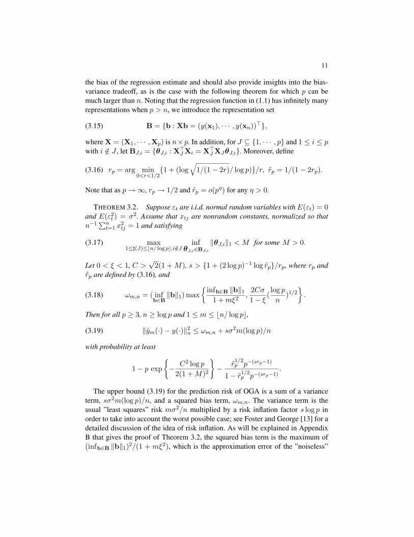
the bias of the regression estimate and should also provide insights into the bias-variance tradeoff, as is the case with the following theorem for which p can bemuch larger than n. Noting that the regression function in (1.1) has infinitely manyrepresentations when p > n, we introduce the representation set

B = b : Xb = (y(x1), · · · , y(xn))>,(3.15)

where X = (X1, · · · ,Xp) is n×p. In addition, for J ⊆ 1, · · · , p and 1 ≤ i ≤ pwith i /∈ J , let BJ,i = θJ,i : X>J Xi = X>J XJθJ,i. Moreover, define

rp = arg min0<r<1/2

1 + (log√

1/(1− 2r)/ log p)/r, rp = 1/(1− 2rp).(3.16)

Note that as p→∞, rp → 1/2 and rp = o(pη) for any η > 0.

THEOREM 3.2. Suppose εt are i.i.d. normal random variables with E(εt) = 0and E(ε2t ) = σ2. Assume that xtj are nonrandom constants, normalized so thatn−1∑n

t=1 x2tj = 1 and satisfying

max1≤](J)≤bn/ log pc,i/∈J

infθJ,i∈BJ,i

‖θJ,i‖1 < M for some M > 0.(3.17)

Let 0 < ξ < 1, C >√

2(1 + M), s > 1 + (2 log p)−1 log rp/rp, where rp andrp are defined by (3.16), and

ωm,n = ( infb∈B‖b‖1) max

infb∈B ‖b‖1

1 +mξ2,

2Cσ1− ξ

(log pn

)1/2.(3.18)

Then for all p ≥ 3, n ≥ log p and 1 ≤ m ≤ bn/ log pc,

‖ym(·)− y(·)‖2n ≤ ωm,n + sσ2m(log p)/n(3.19)

with probability at least

1− p exp

− C2 log p

2(1 +M)2

− r

1/2p p−(srp−1)

1− r1/2p p−(srp−1).

The upper bound (3.19) for the prediction risk of OGA is a sum of a varianceterm, sσ2m(log p)/n, and a squared bias term, ωm,n. The variance term is theusual ”least squares” risk mσ2/n multiplied by a risk inflation factor s log p inorder to take into account the worst possible case; see Foster and George [13] for adetailed discussion of the idea of risk inflation. As will be explained in AppendixB that gives the proof of Theorem 3.2, the squared bias term is the maximum of(infb∈B ‖b‖1)2/(1 + mξ2), which is the approximation error of the ”noiseless”

12

OGA and decreases asm increases, and 2Cσ(1−ξ)−1 infb∈B ‖b‖1(n−1 log p)1/2,which is the error caused by the discrepancy between the noiseless OGA and thesample OGA.

The ‖θJ,i‖1 function in (3.17) is closely related to the cumulative coherencefunction introduced in Tropp [23]. Since Theorem 3.2 does not put any restric-tion on M and infb∈B ‖b‖1, the theorem can be applied to any design matrixalthough a large value of M or infb∈B ‖b‖1 will result in a large bound on theright-hand side of (3.19). When M and infb∈B ‖b‖1 are bounded by a positiveconstant independent of n and p, the upper bound in (3.19) suggests that choosingm = D(n/ log p)1/2 for some D > 0 can provide the best bias-variance tradeoff,for which (3.19) reduces to

‖ym(·)− y(·)‖2n ≤ d(n−1 log p)1/2,(3.20)

where d does not depend on n and p. We can regard (3.20) as an analog of the oracleinequality of Bickel et al. [1, Theorem 6.2] for the Lasso predictor yLasso(r)(xt) =x>t βLasso(r), where

βLasso(r) = arg minc∈Rpn−1

n∑t=1

(yt − x>t c)2 + 2r‖c‖1,(3.21)

with r > 0. Let M(b) denote the number of nonzero components of b ∈ B,and define Q = infb∈BM(b). Instead of (3.17), Bickel et al. [1] assume thatσ is known and X>X satisfies a restricted eigenvalue assumption RE(Q, 3), andshow under the same assumptions of Theorem 3.2 (except for (3.17)) that for r =Aσ(n−1 log p)1/2 with A > 2

√2,

‖yLasso(r)(·)− y(·)‖2n ≤ FQ log pn

,(3.22)

where F is a positive constant depending only on A, σ and 1/κ, in which κ =κ(Q, 3) is the defining restricted engenvalue of RE(Q, 3).

Suppose that F in (3.22) is bounded by a constant independent of n and pand that log p is small relative to n. Then (3.20) and (3.22) suggest that the riskbound for Lasso is smaller (or larger) than that of OGA if Q << (n/ log p)1/2 (orQ >> (n/ log)1/2). To see this, note that when the underlying model has a sparserepresentation in the sense that Q << (n/ log p)1/2, Lasso provides a sparse so-lution that can substantially reduce the approximation error. However, when themodel does not have a sparse representation, Lasso tends to give a relatively non-sparse solution in order to control the approximation error, which also results inlarge variance. In addition, while the RE assumption is quite flexible, the value ofσ, which is required for obtaining βLasso(r) with r = Aσ(n−1 log p)1/2, is usually

13

unknown in practice. On the other hand, although the ability of OGA to reducethe approximation error is not as good as Lasso due to its stepwise local optimiza-tion feature, it has advantages in non-sparse situations by striking a good balancebetween the variance and squared bias with the choice m = D(n/ log p)1/2 in(3.20).

Note that Theorems 3.1 and 3.2 consider weakly sparse regression models thatallow all p regression coefficients to be nonzero. A standard method to select thenumber m of input variables to enter the regression model is cross-validation (CV)or its variants such as Cp and AIC that aim at striking a suitable balance betweensquared bias and variance. However, these variable selection methods do not workwell when p >> n, as shown in [8] that proposes to modify these criteria byincluding a factor log p in order to alleviate overfitting problems.

4. Consistent model selection under strong sparsity. In the case of a fixednumber p (not growing with n) of input variables, only q (< p) of which havenonzero regression coefficients, it is well known that AIC or CV does not penal-ize the residual sum of squares enough for consistent variable selection, for whicha larger penalty (e.g., that used in BIC) is needed. When p = pn → ∞ but thenumber of nonzero regression coefficients remains bounded, Chen and Chen [7]have shown that BIC does not penalize enough and have introduced a consider-ably larger penalty to add to the residual sum of squares so that their ”extendedBIC” is variable selection consistent when pn = O(nκ) for some κ > 0 and anasymptotic identifiability condition is satisfied. As in Section 3.1, we assume herethat log pn = o(n) and also allow the number of nonzero regression coefficients toapproach∞ as n → ∞. To achieve consistency of variable selection, some lowerbound (which may approach 0 as n → ∞) on the absolute values of nonzero re-gression coefficients needs to be imposed. This consideration leads to the followingstrong sparsity condition:

(C5) There exist 0 ≤ γ < 1 such that nγ = o((n/ log pn)1/2) and

lim infn→∞

nγ min1≤j≤pn:βj 6=0

β2j σ

2j > 0.

Note that (C5) imposes a lower bound on β2j σ

2j for nonzero βj . This is more

natural than a lower bound on |βj | since the predictor of yi involves βjxij . Insteadof imposing an upper bound on the number of nonzero regression coefficients asin [7], we show under the strong sparsity condition (C5) that all relevant regres-sors (i.e., those with nonzero regression coefficients) are included by OGA, withprobability near 1 if the number Kn of iterations is large enough. Letting

Nn = 1 ≤ j ≤ pn : βj 6= 0, Dn = Nn ⊆ JKn,(4.1)

14

note that the set JKn of variables selected along an OGA path includes all relevantregressors on Dn.

THEOREM 4.1. Assume (C1)-(C5) and (3.2). SupposeKn/nγ →∞ andKn =

O((n/ log pn)1/2). Then limn→∞ P (Dn) = 1.

PROOF. Without loss of generality, assume that σj = 1 so that zj = xj for1 ≤ j ≤ pn. Let a > 0 and define An(m) by (3.8) in which m = banγc = o(Kn).By (3.8) and (3.12),

limn→∞

P (Acn(m)) ≤ limn→∞

P (Acn(Kn)) = 0,

En[y(x)− yJm(x)]2IAn(m) ≤ C∗m−1.(4.2)

From (4.2), it follows that

limn→∞

P (Fn) = 0,where Fn = En[y(x)− yJm(x)]2 > C∗m−1.(4.3)

For J ⊆ 1, · · · , pn and j ∈ J , let βj(J) be the coefficient of xj in thebest linear predictor

∑i∈J βi(J)xi of y that minimizes E(y−

∑i∈J cixi)

2. Defineβj(J) = 0 if j /∈ J . Note that

En[y(x)− yJm(x)]2 = En∑

j∈Jm∪Nn

(βj − βj(Jm))xj2.(4.4)

From (C4) and (C5), it follows that ](Nn) = o(nγ/2), yielding ](Jm ∪ Nn) =o(Kn). Let vn = min1≤](J)≤Kn λmin(Γ(J)). Then we obtain from (4.4) that forall large n,

En[y(x)− yJm(x)2] ≥ vn minj∈Nn

β2j on Nn ∩ Jcm 6= ∅.(4.5)

Combining (4.5) with (C5) and (3.2) then yields for some b > 0 and all largen, En[y(x) − yJm(x)2] ≥ bn−γ on Nn ∩ Jcm 6= ∅. By choosing the a inm = banγc large enough, we have bn−γ > C∗m−1, implying that Nn ∩ Jcm 6=∅ ⊆ Fn, where Fn is defined in (4.3). Hence by (4.3), limn→∞ P (Nn ⊆ Jm) =1. Therefore, the OGA that terminates after m = banγc iterations contains allrelevant regressors with probability approaching 1. This is also true for the OGAthat terminates after Kn iterations if Kn/m→∞.

Under strong sparsity, we next show that the best fitting model can be cho-sen along an OGA path by minimizing a high-dimensional information criterion

15

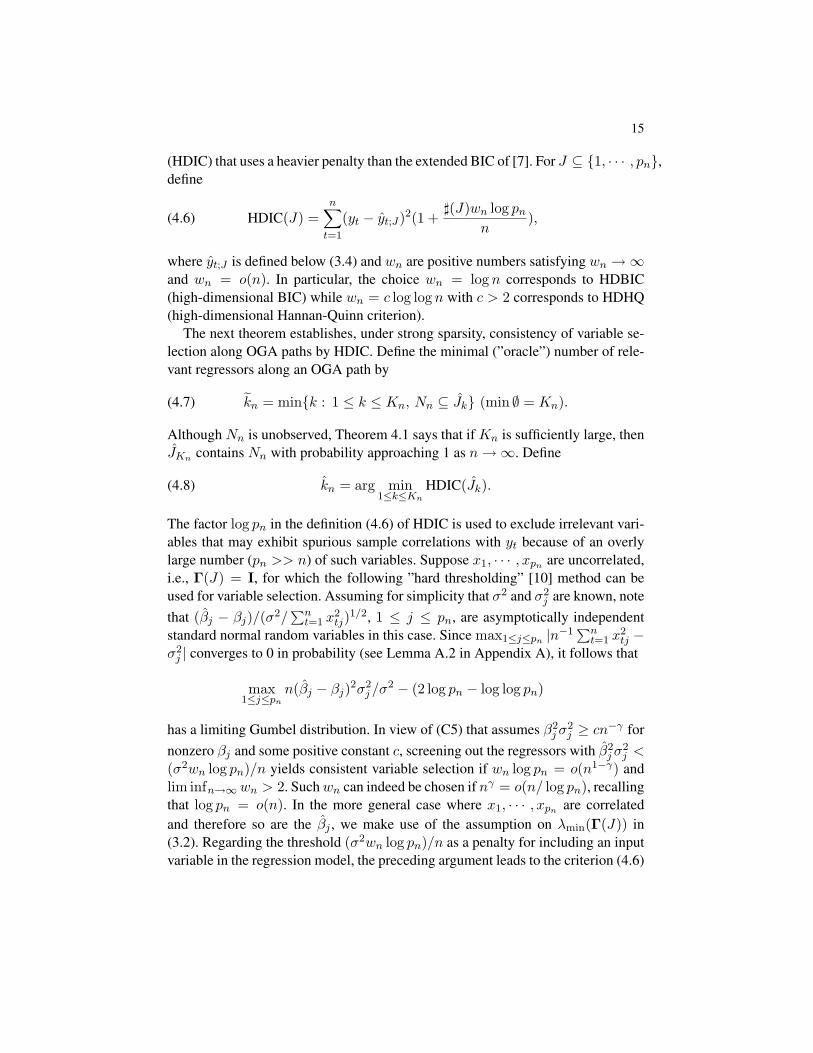
(HDIC) that uses a heavier penalty than the extended BIC of [7]. For J ⊆ 1, · · · , pn,define

HDIC(J) =n∑t=1

(yt − yt;J)2(1 +](J)wn log pn

n),(4.6)

where yt;J is defined below (3.4) and wn are positive numbers satisfying wn →∞and wn = o(n). In particular, the choice wn = log n corresponds to HDBIC(high-dimensional BIC) while wn = c log logn with c > 2 corresponds to HDHQ(high-dimensional Hannan-Quinn criterion).

The next theorem establishes, under strong sparsity, consistency of variable se-lection along OGA paths by HDIC. Define the minimal (”oracle”) number of rele-vant regressors along an OGA path by

(4.7) kn = mink : 1 ≤ k ≤ Kn, Nn ⊆ Jk (min ∅ = Kn).

Although Nn is unobserved, Theorem 4.1 says that if Kn is sufficiently large, thenJKn contains Nn with probability approaching 1 as n→∞. Define

(4.8) kn = arg min1≤k≤Kn

HDIC(Jk).

The factor log pn in the definition (4.6) of HDIC is used to exclude irrelevant vari-ables that may exhibit spurious sample correlations with yt because of an overlylarge number (pn >> n) of such variables. Suppose x1, · · · , xpn are uncorrelated,i.e., Γ(J) = I, for which the following ”hard thresholding” [10] method can beused for variable selection. Assuming for simplicity that σ2 and σ2

j are known, notethat (βj − βj)/(σ2/

∑nt=1 x

2tj)

1/2, 1 ≤ j ≤ pn, are asymptotically independentstandard normal random variables in this case. Since max1≤j≤pn |n−1∑n

t=1 x2tj −

σ2j | converges to 0 in probability (see Lemma A.2 in Appendix A), it follows that

max1≤j≤pn

n(βj − βj)2σ2j /σ

2 − (2 log pn − log log pn)

has a limiting Gumbel distribution. In view of (C5) that assumes β2j σ

2j ≥ cn−γ for

nonzero βj and some positive constant c, screening out the regressors with β2j σ

2j <

(σ2wn log pn)/n yields consistent variable selection if wn log pn = o(n1−γ) andlim infn→∞wn > 2. Suchwn can indeed be chosen if nγ = o(n/ log pn), recallingthat log pn = o(n). In the more general case where x1, · · · , xpn are correlatedand therefore so are the βj , we make use of the assumption on λmin(Γ(J)) in(3.2). Regarding the threshold (σ2wn log pn)/n as a penalty for including an inputvariable in the regression model, the preceding argument leads to the criterion (4.6)

16

and suggests selecting the regressor set J that minimizes HDIC(J). Under (C5) and(3.2), it can be shown that if wn is so chosen that

wn →∞, wn log pn = o(n1−2γ),(4.9)

then the minimizer of HDIC(J) over J with J ⊆ JKn is consistent for variable se-lection. Note that the penalty used in HDIC is heavier than that used in the extendedBIC of [7], and instead of all subset models used in [7], HDIC is applied to modelsafter greedy forward screening, which may result in stronger spurious correlationsamong competing models. The proof is similar to that of the following theorem,which focuses on consistent variable selection along OGA paths, J1, · · · , JKn . Inpractice, it is not feasible to minimize HDIC(J) over all subsets J of JKn whenKn is large, and a practical alternative is to minimize HDIC(Jk) instead.

THEOREM 4.2. With the same notation and assumptions as in Theorem 4.1,suppose (4.9) holds, Kn/n

γ →∞ and Kn = O((n/ log pn)1/2). Then

limn→∞

P (kn = kn) = 1.

PROOF. As in the proof of Theorem 4.1, assume σ2j = 1. For notational sim-

plicity, we drop the subscript n in kn and kn. We first show that P (k < k) = o(1).As shown in the proof of Theorem 4.1, for sufficiently large a,

limn→∞

P (Dn) = 1, where Dn = Nn ⊆ Jbanγc = k ≤ anγ.(4.10)

On k < k, HDIC(Jk) ≤ HDIC(Jk) and∑nt=1(yt − yt;Jk

)2 ≥∑nt=1(yt −

yt;Jk−1)2, so

n∑t=1

(yt − yt;Jk−1)2 −

n∑t=1

(yt − yt;Jk)2

≤ n−1wn(log pn)(k − k)n∑t=1

(yt − yt;Jk)2.(4.11)

Let HJ denote the projection matrix associated with projections into the linearspace spanned by Xj , j ∈ J ⊆ 1, · · · , p. Then

n−1n∑t=1

(yt − yt;Jk−1)2 −

n∑t=1

(yt − yt;Jk)2

= n−1(βjkXjk+ ε)>(HJk

−HJk−1)(βjkXjk

+ ε)

= βjkX>jk

(I−HJk−1)Xjk

+ X>jk

(I−HJk−1)ε2/nX>

jk(I−HJk−1

)Xjk.

(4.12)

17

Simple algebra shows that the last expression in (4.12) can be written as β2jkAn +

2βjkBn + A−1n B2

n, where

An = n−1X>jk

(I−HJk−1)Xjk

, Bn = n−1X>jk

(I−HJk−1)ε,

Cn = n−1n∑t=1

(yt − yt;Jk)2 − σ2.(4.13)

Hence, (4.12) and (4.11) yield β2jkAn + 2βjkBn + A−1

n B2n ≤ n−1wn(log pn)(k −

k)(Cn + σ2) on k < k, which implies that

2βjkBn − n−1wn(log pn)banγc|Cn|

≤ −β2jkAn + n−1wn(log pn)banγcσ2 on k < k

⋂Dn.

(4.14)

Define vn = min1≤](J)≤banγc λmin(Γ(J)). Note that by (3.2), there exists c0 > 0such that for all large n, vn > c0. In Appendix A, it will be shown that for anyθ > 0,

P (An ≤ vn/2,Dn) + P (|Bn| ≥ θn−γ/2,Dn)

+ P (wn(log pn)|Cn| ≥ θn1−2γ ,Dn) = o(1).(4.15)

From (C5), (4.10), (4.14) and (4.15), it follows that P (k < k) = o(1).It remains to prove P (k > k) = o(1). Noting that k < Kn and βj = 0 for

j /∈ Jk, we have the following counterpart of (4.11) and (4.12) on Kn ≥ k > k:

ε>(I−HJk)ε(1 + n−1kwn log pn) ≤ ε>(I−HJk

)ε(1 + n−1kwn log pn),

which implies

ε>(HJk−HJk

)ε(1 + n−1kwn log pn)

≥ n−1ε>(I−HJk)ε(k − k)wn log pn.

(4.16)

Let Fk,k denote the n× (k− k) matrix whose column vectors are Xj , j ∈ Jk− Jk.Standard calculations yield

ε>(HJk−HJk

)ε

= ε>(I−HJk)Fk,kF

>k,k

(I−HJk)Fk,k

−1F>k,k

(I−HJk)ε

≤ ‖Γ−1(JKn)‖‖n−1/2F>

k,k(I−HJk

)ε‖2

≤ 2‖Γ−1(JKn)‖‖n−1/2F>

k,kε‖2 + 2‖Γ−1

(JKn)‖‖n−1/2F>k,k

HJkε‖2

≤ 2(k − k)(an + bn),

(4.17)

18

where Γ(J) denotes the sample covariance matrix that estimates Γ(J) for J ⊆1, · · · , pn (recalling that σ2

j = 1), ‖L‖ = sup‖x‖=1 ‖Lx‖ for a nonnegativedefinite matrix L, and

an = ‖Γ−1(JKn)‖ max

1≤j≤pn(n−1/2

n∑t=1

xtjεt)2,

bn = ‖Γ−1(JKn)‖ max

1≤](J)≤k,i/∈J(n−1/2

n∑t=1

εtxti;J)2.

Since n−1ε>(I−HJk)ε− σ2 = Cn, combining (4.17) with (4.16) yields

2(k − k)(an + bn)(1 + n−1kwn log pn) + |Cn|(k − k)wn log pn

≥ σ2(k − k)wn log pn.(4.18)

In Appendix A it will be shown that for any θ > 0,

P(an + bn)(1 + n−1Knwn log pn) ≥ θwn log pn+ P|Cn| ≥ θ = o(1).

(4.19)

From (4.18) and (4.19), the desired conclusion P (k > k) = o(1) follows.

5. Simulation studies and discussion. In this section, we report simulationstudies of the performance of OGA+HDBIC and OGA+HDHQ. These simulationstudies consider the regression model

(5.1) yt =q∑j=1

βjxtj +p∑

j=q+1

βjxtj + εt, t = 1, · · · , n,

where βq+1 = · · · = βp = 0, p >> n, εt are i.i.d. N(0, σ2) and are independent ofthe xtj . Examples 1 and 2 consider the case

(5.2) xtj = dtj + ηwt,

in which η ≥ 0 and (dt1, · · · , dtp, wt)>, 1 ≤ t ≤ n, are i.i.d. normal with mean(1, · · · , 1, 0)> and covariance matrix I. Since for any J ⊆ 1, · · · , p and 1 ≤ i ≤p with i /∈ J ,

λmin(Γ(J)) = 1/(1 + η2) > 0 and ‖Γ−1(J)gi(J)‖1 ≤ 1,(5.3)

(3.2) is satisfied; moreover, Corr(xtj , xtk) = η2/(1 + η2) increases with η > 0.On the other hand,

(5.4) max1≤](J)≤ν

λmax(Γ(J)) = (1 + νη2)/(1 + η2).

19

As noted in Section 1, Fan and Lv [12] require λmax(Γ(1, · · · , p)) ≤ cnr forsome c > 0 and 0 ≤ r < 1 in their theory for the sure independence screeningmethod, but this fails to hold for the equi-correlated regressors (5.2) when η > 0and p >> n, in view of (5.4). For nonrandom regressors for which there is nopopulation correlation matrix Γ(J) and the sample version Γ(J) is nonrandom,Zhang and Huang [25] have shown that under the sparse Riesz condition c∗ ≤min1≤](J)≤q∗ λmin(Γ(J)) ≤ max1≤](J)≤q∗ λmax(Γ(J)) ≤ c∗ for some c∗ ≥ c∗ >0 and q∗ ≥ 2 + (4c∗/c∗)q + 1, the set of regressors selected by Lasso includesall relevant regressors, with probability approaching 1. If these fixed regressors areactually a realization of (5.2), then in view of (5.3) and (5.4), the requirement thatq∗ ≥ 2 + (4c∗/c∗)q + 1 in the sparse Riesz condition is difficult to meet whenq ≥ (2η)−2.

Example 1. Consider (5.1) with q = 5, (β1, · · · , β5) = (3,−3.5, 4,−2.8, 3.2)and assume that σ = 1 and (5.2) holds. The special case η = 0, σ = 1 or 0.1,and (n, p) = (50, 200) or (100, 400) was used by Shao and Chow [20] to illus-trate the performance of their variable screening method. The cases η = 0, 2 and(n, p) = (50, 1000), (100, 2000), (200, 4000) are considered here to accommo-date a much larger number of candidate variables and allow substantial correlationsamong them. In light of Theorem 4.2 which requires the numberKn of iterations tosatisfy Kn = O((n/ log pn)1/2), we choose Kn = 5(n/ log pn)1/2. Table 1 showsthat OGA+HDBIC and OGA+HDHQ perform well, in agreement with the asymp-totic theory of Theorem 4.2. Each result is based on 1000 simulations. Here and inthe sequel, we choose c = 2.01 for HDHQ. For comparison, the performance ofOGA+BIC is also included in the table.

In the simulations for n ≥ 100, OGA always includes the 5 relevant regressorswithin Kn iterations, and HDBIC and HDHQ identify the smallest correct modelfor 99% or more of the simulations, irrespective of whether the candidate regres-sors are uncorrelated (η = 0) or highly correlated (η = 2). In contrast, OGA+BICalways chooses the model obtained at the last iteration. The mean squared pre-diction errors (MSPE) of OGA+BIC are at least 20 times higher than those ofOGA+HDBIC or OGA+HDHQ when n = 100, and are at least 35 times higherwhen n = 200, where

MSPE =1

1000

1000∑l=1

(p∑j=1

βjx(l)n+1,j − y

(l)n+1)2,

in which x(l)n+1,1, · · · , x

(l)n+1,p are the regressors associated with y(l)

n+1, the new out-

come in the lth simulation run, and y(l)n+1 denotes the predictor of y(l)

n+1. Note thatthe MSPEs of OGA+HDBIC and OGA+HDHQ are close to the ideal value 5σ2/nof (1.3) for the least squares predictor based on only the q = 5 relevant variablesin (5.1).

20

In the case of n = 50 and p = 1000, OGA can include all relevant regressors(within Kn iterations) about 94% of the time when η = 0; this ratio decreasesto 83% when η = 2. As shown in Table 2 of [20], in the case of n = 100 andp = 400, the variable screening method of Shao and Chow [20], used in conjunc-tion with AIC or BIC, can only identify the smallest correct model about 50% ofthe time even when η = 0. To examine the sensitivity of Kn in our simulationstudy, we have varied the value of D in Kn = D(n/ log pn)1/2 from 3 to 10. Theperformance of OGA+HDBIC and OGA+HDHQ remains similar to the case ofD = 5, but that of OGA+BIC becomes worse as D becomes larger.

Example 2. Consider (5.1) with q = 9, n = 400, p = 4000, (β1, · · · , βq)=(3.2,3.2, 3.2, 3.2, 4.4, 4.4, 3.5, 3.5, 3.5) and assume that σ2 = 2.25 and (5.2) holds withη = 1. Table 2 summarizes the results of 1000 simulations on the performanceof Lasso, OGA+HDBIC and OGA+HDHQ, using Kn = 5(n/ log p)1/2 iterations

for OGA. The Lasso estimate βL

(λ) = (βL1 (λ), · · · , βLp (λ))> is defined as theminimizer of n−1∑n

t=1(yt − x>t c)2 + λ‖c‖1 over c. To implement Lasso, we usethe Glmnet package of [15] and conduct 5-fold cross-validation to select the opti-mal λ, yielding the estimate ”Lasso” in Table 2. In addition, we have also tracedthe Lasso path using a modification of the LARS algorithm [11, Section 3] basedon the MATLAB code of [19], and the tracing is stopped when the value of theregularization parameter defined in [19] along the path is smaller than the defaulttolerance of 10−5 or 10−4, yielding the estimate ”LARS(10−5)” or ”LARS(10−4)”in Table 2. We have also tried other default tolerance values 10−1, 10−2, · · · , 10−8,but the associated performance is worse than that of LARS(10−4) or LARS(10−5).Table 2 shows that OGA+HDBIC and OGA+HDHQ can identify the smallest cor-rect model in 98% of the time and choose slightly overfitting models in 2% of thetime. Their MSPEs are near the oracle value qσ2/n = 0.051. Although Lasso orLARS-based implementation of Lasso can include the 9 relevant variables in allsimulation runs, they encounter overfitting problems. The model chosen by Lassois usually more parsimonious than that chosen by LARS (10−4) or LARS(10−5).However, the MSPE of Lasso is larger than those of LARS(10−5) and Lasso(10−4),which are about 10-12 times larger than qσ2/n due to overfitting.

This example satisfies the neighborhood stability condition, introduced in [18],which requires that for some 0 < δ < 1 and all i = q + 1, · · · , p,

|c′qiR−1(q)sign(β(q))| < δ,(5.5)

where xt(q) = (xt1, · · · , xtq)>, cqi = E(xt(q)xti), R(q) = E(xt(q)x>t (q))and sign(β(q)) = (sign(β1), · · · , sign(βq))>. To show that (5.5) holds in thisexample, straightforward calculations give cqi = η21q, R−1(q) = I − η2/(1 +η2q)1q1>q , and sign(β(q)) = 1q, where 1q is the q-dimensional vector of 1’s.Therefore, for all i = q+ 1, · · · , p, |c′qiR−1(q)sign(β(q))| = η2q/(1 + η2q) < 1.

21

TABLE 1Frequency, in 1000 simulations, of selecting all 5 relevant variables in Example 1

η n p Method E E+1 E+2 E+3 E+4 E+5 E∗ Correct MSPE0 50 1000 OGA+HDBIC 902 33 7 0 0 0 0 942 2.99

OGA+HDHQ 864 64 13 3 1 0 0 945 2.90OGA+BIC 0 0 0 0 0 0 945 945 4.87

100 2000 OGA+HDBIC 1000 0 0 0 0 0 0 1000 0.053OGA+HDHQ 994 6 0 0 0 0 0 1000 0.055OGA+BIC 0 0 0 0 0 0 1000 1000 1.245


2 50 1000 OGA+HDBIC 663 121 41 5 0 0 0 830 9.43OGA+HDHQ 643 134 44 17 4 1 0 843 8.36OGA+BIC 0 0 0 0 0 0 843 843 12.59



1. E denotes the frequency of selecting exactly all relevant variables.2. E+i denotes the frequency of selecting all relevant variables and i additional irrelevant variables.3. E∗ denotes the frequency of selecting the largest model along the OGA path which includes all relevant variables.4. Correct denotes the frequency of including all relevant variables.

TABLE 2Frequency, in 1000 simulations, of selecting all 9 relevant variables in Example 2

MethodE E+1 E+2 E+3 Correct MSPE

OGA+HDBIC 980 19 1 0 1000 0.052OGA+HDHQ 980 19 1 0 1000 0.052

Range Average Correct MSPELARS(10−5) [44, 389] 124.3 1000 0.602LARS(10−4) [30, 227] 82.6 1000 0.513Lasso [25, 84] 50.17 1000 0.864

1. The lower and upper limits of range are the smallest and largest numbers of selected variables in 1000 runs.2. Average is the mean number of selected variables over 1000 runs.3. See the footnotes of Table 1 for the notations E, E+i, and Correct.

22

TABLE 3Frequency, in 1000 simulations, of selecting all 10 relevant variables in Example 3 using

the same notation as that in Table 2Method

E E+1 E+2 E+3 Correct MSPEOGA+HDBIC 0 43 939 18 1000 0.033OGA+HDHQ 0 43 939 18 1000 0.033

Range Average Correct MSPELARS(10−7) [325, 439] 408.3 116 10.52LARS(10−5) [81, 427] 331.9 34 1.39Lasso [163, 236] 199.1 0 0.92

Under (5.4) and some other conditions, Meinshausen and Buhlmann [19, Theorems1 and 2] have shown that if λ = λn in β

L(λ) converges to 0 at a rate slower than

n−1/2, then limn→∞ P (Ln(λ) = Nn) = 1, where Ln(λ) = i : βLi (λ) 6= 0.Example 3. Consider (5.1) with q = 10, n = 400, p = 4000 and (β1, · · · , βq)=

(3, 3.75, 4.5, 5.25, 6, 6.75, 7.5, 8.25, 9, 9.75). Assume that σ = 1, that xt1, · · · , xtqare i.i.d. standard normal, and that

xtj = dtj + bq∑l=1

xtl, for q + 1 ≤ j ≤ p,

where b = (3/4q)1/2 and (dt(q+1), · · · , dtp)> are i.i.d. multivariate normal withmean 0 and covariance matrix (1/4)I and are independent of xtj for 1 ≤ j ≤ q.Using the same notation as in the last paragraph of Example 2, straightforwardcalculations show that for q + 1 ≤ j ≤ p, cqj = (b, · · · , b)>, R(q) = I andsign(β(q)) = (1, · · · , 1)>. Therefore, for q+1 ≤ j ≤ p, |c>qjR−1(q)sign(β(q))| =(3q/4)1/2 = (7.5)1/2 > 1, and hence (5.5) is violated. On the other hand, it is notdifficult to show that (3.2) is satisfied in this example.

Table 3 gives the results of 1000 simulations on the performance of Lasso,LARS(10−7), LARS(10−5), OGA+HDBIC and OGA+HDHQ, usingKn = 5(n/ log p)1/2

iterations for OGA. The table shows that LARS (10−7) only includes all 10 rele-vant regressors in 116 of the 1000 simulations, LARS (10−5) includes them in only34 simulations and Lasso fails to include them in all simulations. This result sug-gests that violation of (5.5) seriously degrades Lasso’s ability in variable selection.Despite its inferiority in including all relevant variables, Lasso has MSPE equal to0.92, which is two thirds of the MSPE of LARS(10−5) and is about 11 times lowerthan the MSPE of LARS(10−7). In contrast, OGA+HDBIC and OGA+HDHQ canpick up all 10 relevant regressors and include at most three irrelevant ones. More-over, the MSPEs of OGA+HDBIC and OGA+HDHQ are only slightly larger thanqσ2/n = 0.025.

In Example 1, p is 20 times larger than n and in Examples 2 and 3, (n, p) =

23

(400, 4000). In these examples, the number of relevant regressors ranges from 5 to10 and OGA includes nearly all of them after only 5(n/ log p)1/2 iterations. Thiscomputationally economical feature is attributable to the greedy variable selector(2.1) and the fact that, unlike PGA, a selected variable enters the model only onceand is not re-selected later. Although OGA requires least squares regression of yton all selected regressors, instead of regressing U (k)

t on the most recently selectedregressor as in PGA, the iterative nature of OGA enables us to avoid the computa-tional task of solving a large system of linear normal equations for the least squaresestimates, by sequently orthogonalizing the input variables so that the OGA update(2.3) is basically componentwise linear regression, similar to PGA.

The HDIC used in conjunction with OGA can be viewed as backward elimina-tion after forward stepwise inclusion of variables by OGA. Example 1 shows thatif BIC is used in lieu of HDBIC, then the backward elimination still leaves all in-cluded variables in the model. This is attributable to p being 20 times larger thann, resulting in many spuriously significant regression coefficients if one does notadjust for multiple testing. The factor wn log pn in the definition (4.6) of HDIC canbe regarded as such adjustment, as explained in the paragraph preceding Theorem4.2 that establishes the oracle property of OGA+HDIC under the strong sparsityassumption (C5).

It should be mentioned that since Lasso can include all relevant variables inExample 2, the overfitting problem of Lasso can be substantially rectified if oneperforms Zou’s [28] adaptive Lasso procedure that uses Lasso to choose an initialset of variables for further refinement. On the other hand, in situations where it isdifficult for Lasso to include all relevant variables as in Example 3, such two-stagemodification does not help to improve Lasso.

APPENDIX A: PROOF OF (3.8), (3.13), (4.15) AND (4.19)

The proof of (3.8) relies on the representation (3.7), whose right-hand side in-volves (i) a weighted sum of the i.i.d. random variables εt that satisfy (C2) and(ii) the difference between a nonlinear function of the sample covariance matrixof the xtj that satisfy (C3) and its expected value, recalling that we have assumedσj = 1 in the proof of Theorem 3.2. The proof of (3.13) will also make use ofa similar representation. The following four lemmas give exponential bounds formoderate deviation probabilities of (i) and (ii).

LEMMA A.1. Let ε, ε1, · · · , εn be i.i.d. random variables such that E(ε) = 0,E(ε2) = σ2 and (C2) holds. Then, for any constants ani(1 ≤ i ≤ n) and un > 0such that

un max1≤i≤n

|ani|/An → 0 and u2n/An →∞ as n→∞,(A.1)

24

where An =∑ni=1 a

2ni, we have

Pn∑i=1

aniεi > un ≤ exp−(1 + o(1))u2n/(2σ

2An).(A.2)

PROOF. Let eψ(θ) = E(eθε), which is finite for |θ| < t0 by (C2). By the Markovinequality, if θ > 0 and max1≤i≤n |θani| < t0, then

Pn∑i=1

aniεi > un ≤ exp−θun +n∑i=1

ψ(θani).(A.3)

By (A.1) and the Taylor approximationψ(t) ∼ σ2t2/2 as t→ 0, θun−∑ni=1 ψ(θani)

is minimized at θ ∼ un/(σ2An) and has minimum value u2n/(2σ

2An). Putting thisminimum value in (A.3) proves (A.2).

LEMMA A.2. With the same notation and assumptions as in Theorem 3.1 andassuming that σj = 1 for all j so that zj = xj , there exists C > 0 such that

max1≤i,j≤pn

P|n∑t=1

(xtixtj − σij)| > nδn ≤ exp(−Cnδ2n)(A.4)

for all large n, where σij = Cov(xi, xj) and δn are positive constants satisfyingδn → 0 and nδ2n → ∞ as n → ∞. Define Γ(J) by (3.1) and let Γn(J) be thecorresponding sample covariance matrix. Then, for all large n,

P max1≤](J)≤Kn

‖Γn(J)− Γ(J)‖ > Knδn ≤ p2nexp(−Cnδ2n).(A.5)

If furthermore Knδn = O(1), then there exists c > 0 such that

P max1≤](J)≤Kn

‖Γ−1n (J)− Γ−1(J)‖ > Knδn ≤ p2

nexp(−cnδ2n)(A.6)

for all large n, where Γ−1n denotes a generalized inverse when Γn is singular.

PROOF. Since (xti, xtj) are i.i.d. and (C3) holds, the same argument as thatin the proof of Lemma A.1 can be used to prove (A.4) with C < 1/(2Var(xixj)).Letting4ij = n−1∑n

t=1 xtixtj−σij , note that max1≤](J)≤Kn ‖Γn(J)−Γ(J)‖ ≤Kn max1≤i,j≤pn |4ij | and therefore (A.5) follows from (A.4). Since λmin(Γn(J)) ≥λmin(Γ(J))−‖Γn(J)−Γ(J)‖, it follows from (3.2) and (A.5) that the probabilityof Γn(J) being singular is negligible in (A.6), for which we can therefore assumeΓn(J) to be nonsingular.

25

To prove (A.6), denote Γn(J) and Γ(J) by Γ and Γ for simplicity. Making useof Γ

−1 −Γ−1 = Γ−1(Γ− Γ)Γ−1

and Γ = ΓI + Γ−1(Γ−Γ), it can be shownthat ‖Γ−1 − Γ−1‖(1− ‖Γ−1‖‖Γ− Γ‖) ≤ ‖Γ−1‖2‖Γ− Γ‖, and hence

max1≤](J)≤Kn

‖Γ−1 − Γ−1‖(1− max1≤](J)≤Kn

‖Γ−1‖‖Γ− Γ‖)

≤ max1≤](J)≤Kn

‖Γ−1‖2‖Γ− Γ‖.(A.7)

By (3.2), min1≤](J)≤Kn λmin(Γ) ≥ c0 for some positive constant c0 and all largen. Therefore, max1≤](J)≤Kn ‖Γ

−1‖ ≤ c−10 . Let D = supn≥1Knδn and note that

1−(D+1)−1Knδn ≥ (D+1)−1. We use (A.7) to bound Pmax1≤](J)≤Kn ‖Γ−1−

Γ−1‖ > Knδn by

P

max

1≤](J)≤Kn‖Γ−1 − Γ−1‖ > Knδn, max

1≤](J)≤Kn‖Γ−1‖‖Γ− Γ‖ ≤ Knδn

D + 1

+ P

max

1≤](J)≤Kn‖Γ−1‖‖Γ− Γ‖ > Knδn

D + 1

≤ P

max1≤](J)≤Kn

‖Γ−1‖2‖Γ− Γ‖ > KnδnD + 1

+ P

max

1≤](J)≤Kn‖Γ−1‖‖Γ− Γ‖ > Knδn

D + 1

.

(A.8)

Since max1≤](J)≤Kn ‖Γ−1‖2 ≤ c−2

0 , combining (A.8) with (A.5) (in which δn isreplaced by c20δn/(D+1) for the first summand in (A.8), and by c0δn/(D+1)for the second) yields (A.6) with c < Cc40/(D + 1)2.

LEMMA A.3. With the same notation and assumptions as in Theorem 3.1 andassuming σj = 1 for all j, let n1 =

√n/(log n)2 and nk+1 =

√nk for k ≥ 1.

Let un be positive constants such that un/n1 → ∞ and un = O(n). Let K be apositive integer and Ωn = max1≤t≤n |εt| < (log n)2. Then there exists α > 0such that for all large n,

max1≤i≤pn

Pmax1≤t≤n

|xti| ≥ n1 ≤ exp(−αn21),(A.9)

max1≤k≤K,1≤i≤pn

P

(n∑t=1

|εtxti|Ink+1≤|xti|<nk ≥ un(log n)2,Ωn

)≤ exp(−αun).

(A.10)

26

PROOF. (A.9) follows from (C3). To prove (A.10), note that on Ωn,

n∑t=1

|εtxti|Ink+1≤|xti|<nk ≤ nk(log n)2n∑t=1

I|xti|≥nk+1.

Therefore, it suffices to show that for all large n and 1 ≤ i ≤ pn, 1 ≤ k ≤ K,

exp(−αun) ≥ P (n∑t=1

I|xti|≥nk+1 ≥ un/nk) = PBinomial(n, πn,k,i) ≥ un/nk,

where πn,k,i = P (|xi| ≥ nk+1) ≤ exp(−cn2k+1) = exp(−cnk) for some c > 0, by

(C3). The desired conclusion follows from standard bounds for the tail probabilityof a binomial distribution, recalling that un = O(n) and un/n1 →∞.

LEMMA A.4. With the same notation and assumptions as in Lemma A.3, let δnbe positive numbers such that δn = O(n−θ) for some 0 < θ < 1/2 and nδ2n →∞.Then there exists β > 0 such that for all large n,

max1≤i≤pn

P

(|n∑t=1

εtxti| ≥ nδn,Ωn

)≤ exp(−βnδ2n).(A.11)

PROOF. Let ni, i ≥ 1 be defined as in Lemma A.3. Let K be a positive integersuch that 2−K < θ. Then since δn = O(n−θ), n2−K = o(δ−1

n ). Letting A(1) =[n1,∞), A(k) = [nk, nk−1) for 2 ≤ k ≤ K, A(K+1) = [0, nK), note that

P

(|n∑t=1

εtxti| ≥ nδn,Ωn

)

≤K+1∑k=1

P

(|n∑t=1

εtxtiI|xti|∈A(k)| ≥ nδn/(K + 1),Ωn

)≤ P ( max

1≤t≤n|xti| ≥ n1)

+K+1∑k=2

P

(|n∑t=1


).

(A.12)

From (A.10) (in which un is replaced by nδn/(K + 1)(log n)2), it follows thatfor 2 ≤ k ≤ K and all large n,

max1≤i≤pn

P

(|n∑t=1


)

≤ exp− αnδn

(K + 1)(log n)2

,

(A.13)

27

where α is some positive constant. Moreover, by (A.9), max1≤i≤pn P (max1≤t≤n|xti| ≥ n1) ≤ exp −αn/(log n)4, for some α > 0. Putting this bound and(A.13) into (A.12) and noting that 1/(log n)2δn → ∞, it remains to show

max1≤i≤pn

P

(|n∑t=1

εtxtiI|xti|∈A(K+1)| ≥ nδn/(K + 1),Ωn

)≤ exp(−c1nδ2n).

(A.14)

Let 0 < d1 < 1 and Li = d1 ≤ n−1∑nt=1 x

2tiI|xti|∈A(K+1) < d−1

1 . By anargument similar to that used in the proof of (A.4), it can be shown that there existsc2 > 0 such that for all large n, max1≤i≤pn P (Lci ) ≤ exp(−c2n). Applicationof Lemma A.1 after conditioning on Xi, which is independent of (ε1, · · · , εn)>,shows that there exists c3 > 0 for which

max1≤i≤pn

P (|n∑t=1

εtxtiI|xti|∈A(K+1)| ≥ nδn/(K + 1), Li) ≤ exp(−c3nδ2n),

for all large n. This completes the proof of (A.14).

PROOF OF (3.8). Let Ωn = max1≤t≤n |εt| < (log n)2. It follows from (C2)that limn→∞ P (Ωc

n) = 0. Moreover, by (A.4), there exists C > 0 such that for anyd2C > 1 and all large n,

P ( max1≤i≤pn

|n−1n∑t=1

x2ti − 1| > d(log pn/n)1/2))

≤ pnexp(−Cd2 log pn) = explog pn − Cd2 log pn = o(1).

(A.15)

Combining (A.15) with (3.7), (C4) and limn→∞ P (Ωcn) = 0, it suffices for the

proof of (3.8) to show that for some d > 0,

P ( max](J)≤Kn−1,i∈/J

|n−1n∑t=1

εtx⊥ti;J | > d(log pn/n)1/2,Ωn) = o(1),(A.16)

and

P ( maxi,j /∈J,](J)≤Kn−1

|n−1n∑t=1

xtj x⊥ti;J − E(xjx⊥i;J)| > d(log pn/n)1/2)

= o(1).

(A.17)

28

To prove (A.16), let xt(J) be a subvector of xt, with J denoting the correspond-ing subset of indices, and denote Γn(J) by Γ(J) for simplicity. Note that

max](J)≤Kn−1,i/∈J

|n−1n∑t=1

εtx⊥ti;J | ≤ max

1≤i≤pn|n−1

n∑t=1

εtxti|

+ max](J)≤Kn−1,i/∈J

|(n−1n∑t=1

x⊥ti:Jxt(J))>Γ−1

(J)(n−1n∑t=1

εtxt(J))|

+ max](J)≤Kn−1,i/∈J

|g>i (J)Γ−1(J)(n−1n∑t=1

εtxt(J))|

:= S1,n + S2,n + S3,n,

(A.18)

where x⊥ti:J = xti−g>i (J)Γ−1(J)xt(J). Since S3,n ≤max1≤i≤pn |n−1∑nt=1 εtxti|

max](J)≤Kn−1,i/∈J ‖Γ−1(J)gi(J)‖1, by (3.2) and Lemma A.4, there exists β > 0such that for any d > β−1/2(M + 1) and all large n,

P (S1,n + S3,n > d(log pn/n)1/2,Ωn)

≤ pnexp(−βd2 log pn/(M + 1)2) = o(1).(A.19)

Since Kn = O((n/ log n)1/2), there exists c1 > 0 such that for all large n, Kn ≤c1(n/ log pn)1/2. As shown in the proof of Lemma A.2, max1≤](J)≤Kn ‖Γ

−1(J)‖ ≤c−10 for all large n. In view of this and (A.6), there exists c > 0 such that for anyM > (2c21/c)

1/2 and all large n,

P ( max1≤](J)≤Kn

‖Γ−1(J)‖ > c−1

0 + M)

≤ P ( max1≤](J)≤Kn

‖Γ−1(J)− Γ−1(J)‖ > M)

≤ p2nexp(−cnM2/K2

n) = o(1).

(A.20)

By observing

max](J)≤Kn−1,i/∈J

‖n−1n∑t=1

x⊥ti:Jxt(J)‖

≤ K1/2n max

1≤i,j≤pn|n−1

n∑t=1

xtixtj − σij |

× (1 + max1≤](J)≤Kn,i/∈J

‖Γ−1(J)gi(J)‖1),

(A.21)

and max](J)≤Kn−1,i/∈J ‖n−1∑nt=1 εtxt(J)‖ ≤ K1/2

n max1≤i≤pn |n−1∑nt=1 εtxti|,

29

it follows from (3.2) that

S2,n ≤ ( max1≤](J)≤Kn

‖Γ−1(J)‖)Kn(1 +M)

× ( max1≤i,j≤pn

|n−1n∑t=1

xtixtj − σij |)( max1≤i≤pn

|n−1n∑t=1

εtxti|).(A.22)

Define Ω1,n = max1≤](J)≤Kn ‖Γ−1

(J)‖ ≤ c2 = c−10 + M. Then by Lemma

A.4, (A.20), (A.22), (A.4) and Kn = O((n/ log pn)1/2), there exists sufficientlylarge d > 0 such that

P (S2,n > d(log pn/n)1/2,Ωn) ≤ P (Ωc1,n)

+ P

(max

1≤i≤pn|n−1

n∑t=1

εtxti| >d1/2(log pn/n)1/4

(Knc2(1 +M))1/2,Ωn

)

+ P

(max

1≤i,j≤pn|n−1

n∑t=1

xtixtj − σij | >d1/2(log pn/n)1/4

(Knc2(1 +M))1/2

)= o(1).

(A.23)

From (A.18), (A.19) and (A.23), (A.16) follows.We prove (A.17) by using the bound

max](J)≤Kn−1,i,j /∈J

|n−1n∑t=1

xtj x⊥ti;J − E(xjx⊥i;J)|

≤ max1≤i,j≤pn

|n−1n∑t=1

xtjxti − σij |

+ max](J)≤Kn−1,i,j /∈J

|g>j (J)Γ−1(J)n−1n∑t=1

x⊥ti;Jxt(J)|


|g>i (J)Γ−1(J)(n−1n∑t=1

xtjxt(J)− gj(J))|


‖Γ−1(J)‖‖n−1

n∑t=1

x⊥ti;Jxt(J)‖‖n−1n∑t=1

x⊥tj;Jxt(J)‖

:= S4,n + S5,n + S6,n + S7,n.

(A.24)

It follows from (3.2) that S5,n ≤ max1≤i,j≤pn |n−1∑nt=1 xtjxti − σij |(1 +M)M

and S6,n ≤ max1≤i,j≤pn |n−1∑nt=1 xtjxti − σij |M . Combining this with (A.4)

yields that for some d > 0,

P (S4,n + S5,n + S6,n > d(log pn/n)1/2) = o(1).(A.25)

30

In view of (A.21) and (3.2),

S7,n ≤ ( max1≤](J)≤Kn

‖Γ−1(J)‖)Kn(1 +M)2 max

1≤i,j≤pn(n−1

n∑t=1

xtjxti − σij)2.

Therefore, by (A.4) and (A.20), there exists d > 0 such that

P (S7,n > d(log pn/n)1/2) ≤ P (Ωc1,n)

+ P

(max

1≤i,j≤pn(n−1

n∑t=1

xtjxti − σij)2 >d(log pn/n)1/2

c2Kn(1 +M)2

)= o(1).

(A.26)

Consequently, (A.17) follows from (A.24)-(A.26). 2

PROOF OF (3.13). Let q(J) = E(yxJ) and

Q(J) = n−1n∑t=1

(yt − x>t (J)Γ−1(J)q(J))xt(J).

Then, En(ym(x) − yJm(x))2 = Q>(Jm)Γ−1

(Jm)Γ(Jm)Γ−1

(Jm)Q(Jm). Wefirst show that

max1≤m≤Kn

n‖Q(Jm)‖2

m log pn= Op(1).(A.27)

By observing

‖Q(Jm)‖2 ≤ 2m max1≤i≤pn

(n−1n∑t=1

εtxti)2 + 2m max1≤i,j≤pn

(n−1n∑t=1

xtixtj − σij)2

× (pn∑j=1

|βj |)2(1 + max1≤](J)≤Kn,1≤l≤pn

‖Γ−1(J)gl(J)‖1)2,

(A.27) follows from (C4), (3.2), (A.4) and Lemma A.4. By (A.5) and (A.6),

max1≤m≤Kn

‖Γ−1(Jm)‖ = Op(1), max

1≤m≤Kn‖Γ(Jm)− Γ(Jm)‖ = Op(1).

This, (A.27) and the fact that

En(ym(x)− yJm(x))2 ≤ ‖Q(Jm)‖2‖Γ−1(Jm)‖2‖Γ−1

(Jm)− Γ(Jm)‖

+ ‖Q(Jm)‖2‖Γ−1(Jm)‖

together yield the desired conclusion (3.13). 2

31

PROOF OF (4.15). Denote banγc in (4.10) by m0. By (3.2) and an argumentsimilar to that used to prove (A.6) and in (A.20), there exists c1 > 0 such that

P ( max1≤](J)≤m0

‖Γ−1(J)‖ > 2v−1

n ) ≤ p2nexp(−c1n1−2γ) = o(1).(A.28)

Defining Ωn as in Lemma A.3, it follows from (A.16) and (C5) that

P (|Bn| ≥ θn−γ/2,Dn,Ωn)

≤ P ( max](J)≤m0−1,i/∈J

|n−1n∑t=1

εtx⊥ti;J | ≥ θn−γ/2,Ωn) = o(1).

(A.29)

Since (4.9) implies that n1−2γ/(wn log pn) → ∞, it follows from Lemma A.4,(4.9), (3.2) and (A.28) that for all large n,

P (|Cn| ≥ θn1−2γ/(wn log pn),Dn,Ωn)

≤ P (|n−1n∑t=1

ε2t − σ2| ≥ θ/2)

+ P ( max1≤](J)≤m0

‖Γ−1(J)‖m0 max

1≤j≤pn(n−1

n∑t=1

εtxtj)2 ≥ θ/2,Ωn)

= o(1).

(A.30)

As noted above in the proof of (3.8), P (Ωn) = 1 + o(1). Moreover, by (4.9) and(A.5) with Kn replaced by m0, there exists c2 > 0 such that

P (An < vn/2,Dn) ≤ P (λmin(Γ(Jkn)) < vn/2,Dn)

≤ P (λmin(Γ(Jm0)) < vn/2)

≤ P ( max1≤](J)≤m0

‖Γ(J)− Γ(J)‖ > c0/2)

≤ p2nexp(−c2n1−2γ) = o(1),

(A.31)

where c0 is defined in the line following (4.14). In view of (A.29)-(A.31), the de-sired conclusion follows. 2

PROOF OF (4.19). Letting M be defined as in (A.20) and πn = wn(log pn)/(1+wn(log pn)Knn

−1), note that

P(an + bn)(1 + n−1Knwn log pn) ≥ θwn log pn

≤ P (Ωcn) + P (‖Γ−1

(JKn)‖ ≥ c−10 + M)

+ P ( max1≤j≤pn

(n−1/2n∑t=1

xtjεt)2 ≥ πnθ/2(c−10 + M),Ωn)

+ P (2n(S2,n + S3,n)2 ≥ πnθ/2(c−10 + M),Ωn),

(A.32)

32

where S2,n and S3,n are defined in (A.18). SinceKn = O((n/ log pn)1/2), (n/ log pn)1/2 →∞ and wn →∞, there exists ln →∞ such that

πn ≥ 2−1 minwn log pn, nK−1n ≥ ln log pn.(A.33)

By (A.33) and Lemma A.4, we boundP (max1≤j≤pn(n−1/2∑nt=1 xtjεt)

2 ≥ πnθ/2(c−10 +

M),Ωn) by

pn max1≤j≤pn

P (|n−1/2n∑t=1

xtjεt| ≥ (πnθ/2(c−10 + M))1/2,Ωn)

≤ pnexp(−c1ln log pn) = o(1),

for some c1 > 0. By (A.33) and an argument similar to that used in (A.19) and(A.23), it follows that

P (2n(S2,n + S3,n)2 ≥ πnθ/2(c−10 + M),Ωn) = o(1).

In view of (A.20), one also has

P (‖Γ−1(JKn)‖ ≥ c−1

0 + M) = o(1).

Adding these bounds for the summands in (A.32), we obtain

P(an + bn)(1 + n−1Knwn log pn) ≥ θwn log pn = o(1).(A.34)

Form (A.30), (4.10) and P (Ωn) = 1 + o(1), it is straightforward to see thatP (|Cn| ≥ θ) = o(1). Combining this with (A.34) yields (4.19). 2

APPENDIX B: PROOF OF THEOREM 3.2

Note that when the regressors are nonrandom, the population version of OGAis the ”noiseless” OGA that replaces yt in OGA by its mean y(xt). Let µ =(y(x1), · · · , y(xn))>. Let HJ denotes the projection matrix associated with theprojection into the linear space spanned by Xj , j ∈ J ⊆ 1, · · · , p. Let U(0) =µ, j1 = arg max1≤j≤p |(U(0))>Xj |/ ‖Xj‖ and U(1) = (I−Hj1)µ. Proceedinginductively yields

jm = arg max1≤j≤p

|(U(m−1))>Xj |/‖Xj‖,U(m) = (I−Hj1,··· ,jm)µ.

When the procedure stops after m iterations, the noiseless OGA determines anindex set Jm = j1, · · · , jm and approximates µ by HJm

µ. A generalizationof noiseless OGA takes 0 < ξ ≤ 1 and replaces ji by ji,ξ, where ji,ξ is any1 ≤ l ≤ p satisfying |(U(i−1))>Xl|/‖Xl‖ ≥ ξmax1≤j≤p |(U(i−1))>Xj |/‖Xj‖.We first prove the following inequality for such generalization of the noiselessOGA.

33

LEMMA B.1. Let 0 < ξ ≤ 1, m ≥ 1, Jm,ξ = j1,ξ, · · · , jm,ξ and σ2j =

n−1∑nt=1 x

2tj . Then

‖(I−HJm,ξ)µ‖2 ≤ n( inf

b∈B

p∑j=1

|bj σj |)2(1 +mξ2)−1.

PROOF. For J ⊆ 1, · · · , p, i ∈ 1, · · · , p and m ≥ 1, define νJ,i =(Xi)>(I−HJ)µ/(n1/2‖Xi‖). Note that

‖(I−HJm,ξ)µ‖2

≤ ‖(I−HJm−1,ξ)µ−

(µ)>(I−HJm−1,ξ)Xjm,ξ

‖Xjm,ξ‖2

Xjm,ξ‖2

≤ ‖(I−HJm−1,ξ)µ‖2 − nν2

Jm−1,ξ,jm,ξ

≤ ‖(I−HJm−1,ξ)µ‖2 − nξ2 max

1≤j≤pν2Jm−1,ξ,j

,

(B.1)

in which HJ0,ξ= 0. Moreover, for any b = (b1, · · · , bp)> ∈ B,

‖(I−HJm−1,ξ)µ‖2 = n1/2

p∑j=1

bj‖Xj‖νJm−1,ξ,j

≤ max1≤j≤p

|νJm−1,ξ,j|n

p∑j=1

|bj σj |.(B.2)

Let Q = n1/2∑pj=1 |bj σj |. It follows from (B.1) and (B.2) that

‖(I−HJm,ξ)µ‖2 ≤ ‖(I−HJm−1,ξ

)µ‖21− (ξ2‖(I−HJm−1,ξ)µ‖2/Q2).

(B.3)

By Minkowski’s inequality, ‖(I−HJ0,ξ)µ‖2 = ‖µ‖2 ≤ Q2. From this, (B.3) and

Lemma 3.1 of [21], the stated inequality follows. 2

PROOF OF THEOREM 3.2. For the given 0 < ξ < 1, let ξ = 2/(1− ξ),

A = max(J,i):](J)≤m−1,i/∈J

|µJ,i − νJ,i| ≤ Cσ(n−1 log p)1/2,

B = min0≤i≤m−1

max1≤j≤p

|νJi,j | > ξCσ(n−1 log p)1/2,

recalling that µJ,i is defined in (3.4) and νJ,i is introduced in the proof of LemmaB.1. Note that νJ,i, A andB play the same roles as those of µJ,i, An(m) andBn(m)

34

in the proof of Theorem 3.1. By an argument similar to that used to prove (3.10),we have for all 1 ≤ q ≤ m,

|νJq−1,jq| ≥ ξ max

1≤j≤p|νJq−1,j

| on A⋂B,(B.4)

which implies that on the setA⋂B, Jm is the index set chosen by a generalization

of the noiseless OGA. Therefore, it follows from Lemma B.1 that

‖(I−HJm)µ‖2IA⋂B ≤ n( inf

b∈B‖b‖1)2(1 +mξ2)−1.(B.5)

Moreover, for 0 ≤ i ≤ m− 1, ‖(I−HJm)µ‖2 ≤ ‖(I−HJi

)µ‖2 and therefore

‖(I−HJm)µ‖2 ≤ min

0≤i≤m−1

p∑j=1

bjX>j (I−HJi)µ

≤ ( min0≤i≤m−1

max1≤j≤p

|νJi,j |)n‖b‖1 ≤ ξCσ(n log p)1/2‖b‖1 on Bc.

(B.6)

Since A decreases as m increases, it follows from (3.18), (B.5) and (B.6) that

n−1‖(I−HJm)µ‖2IA ≤ ωm,n for all 1 ≤ m ≤ bn/ log pc,(B.7)

where A denotes the set A with m = bn/ log pc. Moreover, as will be shownbelow,

P (Ac) ≤ a∗ := p exp−2−1C2(log p)/(1 +M)2,(B.8)

P (Ec) ≤ b∗ :=r1/2p p−(srp−1)

1− r1/2p p−(srp−1),(B.9)

where E = ε>HJmε ≤ sσ2m log p for all 1 ≤ m ≤ bn/ log pc and rp and

rp are defined in (3.16). By (B.7)-(B.9) and observing that ‖ym(·) − y(·)‖2n =n−1(‖(I−HJm

)µ‖2+ε>HJmε), (3.19) holds on the setA

⋂E , whose probability

is at least 1− a∗ − b∗. Hence the desired conclusion follows. 2

PROOF OF (B.8). Since µJ,i = (Xi)>(I−HJ)Y/(n1/2‖Xi‖) and n−1∑nt=1 x

2tj =

1 for all 1 ≤ j ≤ p, it follows that for any J ⊆ 1, · · · , p, 1 ≤ i ≤ p and i /∈ J ,

|µJ,i − νJ,i| ≤ max1≤i≤p

|n−1n∑t=1

xtiεt|(1 + infθJ,i∈BJ,i

‖θi,J‖1),

setting ‖θJ,i‖1 = 0 if J = ∅. This and (3.17) yield

max](J)≤bn/ log pc−1,i/∈J

|µJ,i − νJ,i| ≤ max1≤i≤p

|n−1n∑t=1

xtiεt|(1 +M).(B.10)

35

By (B.10) and the Gaussian assumption on εt,

P (Ac) ≤ Pmax1≤i≤p

|n−1/2n∑t=1

xtiεt/σ| > C(log p)1/2(1 +M)−1

≤ p exp(−C2 log p/[2(1 +M)2]).

2

PROOF OF (B.9). Clearly P (Ec) ≤∑bn/ log pcm=1 pm max](J)=m P (ε>HJε >

sσ2m log p). Moreover, we can make use of the χ2-distribution to obtain the bound

max](J)=m

P (ε>HJε > sσ2m log p) ≤ exp(−rsm log p)(1− 2r)−m/2(B.11)

for any 0 < r < 1/2. With r = rp and s > 1 + (2 log p)−1 log rp /rp in(B.11), we can use (B.11) to bound P (Ec) by

∑bn/ log pcm=1 gm ≤ g/(1 − g), where

g = r1/2p p−(srp−1) < 1, yielding (B.9). 2

REFERENCES

[1] BICKEL, P., RITOV, Y. and TSYBAKOV, A. (2009). Simultaneous analysis of Lasso and Dantzigselector. Ann. Statist., to appear.

[2] BUHLMANN, P. (2006). Boosting for high-dimensional linear models. Ann. Statist. 34 559-583.[3] BUHLMANN, P. and YU, B. (2003). Boosting with the L2 loss: regression and classification. J.

Amer. Statist. Assoc. 98 324-339.[4] BUNEA F., TSYBAKOV, A.B. and WEGKAMP, M.H. (2007). Sparsity oracle inequalities for the

Lasso. Electronic Journal of Statistics 1 169-194.[5] CANDES, E.J. and TAO, T. (2007). The Dantzig selector: statistical estimation when p is much

larger than n. Ann. Statist. 35 2313-2351.[6] CANDES, E.J. and PLAN, Y. (2009). Near-ideal model selection by l1 minimization. Ann.

Statist. 37 2145-2177.[7] CHEN, J. and CHEN, Z. (2008). Extended Bayesian information criteria for model selection

with large model spaces. Biometrika 95 759-771.[8] CHEN, R.-B., ING, C.-K., LAI, T.L. and ZHANG, F. (2009). Cross-validation in high-

dimensional linear regression models. Tech. Report, Dept. Statistics, Stanford Univ.[9] DONOHO, D.L., ELAD, M. and TEMLYAKOV, V.N. (2006). Stable recovery of sparse overcom-

plete representations in the presence of noise. IEEE Trans. Info. Theory 52 6-18.[10] DONOHO, D.L. and JOHNSTONE, I.M. (1994). Ideal spatial adaptation by wavelet shrinkage.

Biometrika 81 425-455.[11] EFRON, B., HASTIE, T., JOHNSTONE, I. and TIBSHIRANI, R. (2004). Least angle regression

(with discussion). Ann. Statist. 32 407-499.[12] FAN, J. and LV, J. (2008). Sure independence screening for ultra-high dimensional feature

space (with discussion). J. Roy. Statist. Soc. Ser. B 70 849-911.[13] FOSTER, D.P. and GEORGE, E.I. (1994). The risk inflation criterion for multiple regression.

Ann. Statist. 22 1947-1975.[14] FRIEDMAN, J. (2001). Greedy function approximation: a gradient boosting machine. Ann.

Statist. 29 1189-1232.[15] FRIEDMAN, J. , HASTIE, T. and TIBSHIRANI, R (2009). Regularized Paths for Generalized

Linear Models via Coordinate Descent. Technical Report.

36

[16] HANNAN, E.J. and QUINN, B.C. (1979). The determination of the order of an autoregression.J. Roy. Statist. Soc. Ser. B 41 190-195.

[17] MALLAT, S. and ZHANG, Z. (1993). Matching pursuit with time-frequency dictionaries. IEEETrans. Signal Process 41 3397V3415.

[18] MEINSHAUSEN, N. and BUHLMANN, P. (2006). High dimensional graphs and variable selec-tion with the Lasso. Ann. Statist. 34 1436-1462.

[19] ROCHA, G.V. and ZHAO, P. (2006). An implementation of the LARS algorithm for getting theLasso path in MATLAB. http://www.stat.berkeley.edu/∼gvrocha.

[20] SHAO, J. and CHOW, S.-C. (2007). Variable screening in predicting clinical outcome withhigh-dimensional microarrays. J. Multivariate Anal. 98 1529-1538.

[21] TEMLYAKOV, V.N. (2000). Weak greedy algorithms. Adv. Comput. Math. 12 213-227.[22] TIBSHIRANI, R. (1996). Regression shrinkage and selection via the Lasso. J. Roy. Statist. Soc.

Ser. B 58 267-288.[23] TROPP, J.A. (2004). Greed is good: Algorithmic results for sparse approximation. IEEE Trans.

Info. Theory 50 2231-2242.[24] TROPP, J.A. and GILBERT, A.C. (2007). Signal recovery from random measurements via or-

thogonal matching pursuit. IEEE Trans. Info. Theory 53 4655-4666.[25] ZHANG, C.-H. and HUANG, J. (2008). The sparsity and bias of the Lasso selection in high-

dimensional linear regression. Ann. Statist. 36 1567-1594.[26] ZHANG, T. (2009). Some sharp performance bounds for least squares regression with L1 reg-

ularization. Ann. Statist., to appear.[27] ZHAO, P. and YU, B. (2006). On model selection consistency of Lasso. J. Machine Learning

Research 7 2541-2563.[28] ZOU, H. (2006). The adaptive Lasso and its oracle properties. J. Amer. Statist. Assoc. 101

1418-1429.

CHING-KANG INGINSTITUTE OF STATISTICAL SCIENCEACADEMIA SINICATAIPEI 115, TAIWAN, ROCE-MAIL: [email protected]

TZE LEUNG LAIDEPARTMENT OF STATISTICSSTANFORD UNIVERSITYSTANFORD CA94305-4065, USAE-MAIL: [email protected]

A STEPWISE REGRESSION METHOD AND CONSISTENT...

Documents

Transcript of A STEPWISE REGRESSION METHOD AND CONSISTENT...