A Statistical Mechanics Perspective on Glasses and Aging

Ludovic Berthier1 and Giulio Biroli2

1Laboratoire des Colloıdes, Verres et Nanomateriaux,

Universite Montpellier II and CNRS, 34095 Montpellier, France2Service de Physique Theorique Orme des Merisiers – CEA Saclay, 91191 Gif sur Yvette Cedex, France

(Dated: December 4, 2007)

We briefly review the field of the glass transition, glassy dynamics and aging from a statisticalmechanics perspective. We give a broad introduction to the subject and then explain the mainphenomenology and puzzles encountered in glassy systems. We discuss the important role playedby computer simulations to understand the dynamics of systems close to the glass transition at themolecular level. We discuss more particularly the idea of a spatially heterogeneous dynamics thatcharacterizes the relaxation of supercooled liquids. We review the main theoretical approaches thatare currently available to account for these glassy phenomena and discuss the physics of aging andoff-equilibrium dynamics exhibited by glassy materials. We conclude the review by giving someperspectives for future research in the field.

Contents

I. Glossary 1

II. Glasses and aging: a broad introduction 2

III. Phenomenology 3

IV. Taxonomy of ‘glasses’ in science 6

A. The jamming transition of colloids andgrains 6

B. Other ‘glasses’ in physics and beyond 7

V. Numerical simulations 7

VI. Dynamic heterogeneity 9

A. Existence of spatio-temporal dynamicfluctuations 9

B. Multi-point correlation functions 11

VII. Some theory and models 13

A. Cooperativity, chaotic energy landscapesand Random First Order Theory 13

B. Free volume, defects, and facilitated models 16

C. Geometric frustration, avoided criticality,and Coulomb frustrated theories 19

VIII. Aging and off-equilibrium 20

A. Why aging? 20

B. Memory and rejuvenation effects 21

C. Mean-field aging and effective temperatures 22

D. Beyond mean-field 23

E. Driven glassy materials 25

IX. Future directions 26

Acknowledgments 26

References 26

I. GLOSSARY

In this preliminary section, we give a few concise defi-nitions of the most important concepts discussed in thisarticle.

Glass transition–For molecular liquids, the glasstransition denotes a crossover from a viscous liquid toan amorphous solid. Experimentally, the crossover takesplace at the glass temperature, Tg, conventionally definedas the temperature where the liquid’s viscosity reachesthe arbitrary value of 1012 Pa.s. The glass transitionmore generally applies to many different condensed mat-ter systems where a crossover or, less frequently, a truephase transition, takes place between an ergodic phaseand a frozen, amorphous glassy phase.

Aging–In the glass phase, disordered materials arecharacterized by relaxation times that exceed commonobservation timescales, so that a material quenchedin its glass phase never reaches equilibrium (neither ametastable equilibrium). It exhibits instead an aging be-haviour during which its physical properties keep evolv-ing with time.

Dynamic heterogeneity–Relaxation spectra in su-percooled liquids are very broad. This is associated to aspatial distribution of timescales: at any given time, dif-ferent regions in the liquid relax at different rates. Sincethe supercooled liquid is ergodic, slow regions eventu-ally become fast, and vice versa. Dynamic heterogene-ity refers to the existence of these non-trivial spatio-temporal fluctuations in the local dynamical behaviour, aphenomenon observed in virtually all disordered systemswith slow dynamics.

Effective temperature–An aging material relaxesvery slowly, trying (in vain) to reach its equilibrium state.During this process, the system probes states that donot correspond to thermodynamic equilibrium, so that itsthermodynamic properties can not be rigorously defined.Any practical measurement of its temperature becomesa frequency-dependent operation. A ‘slow’ thermome-ter tuned to the relaxation timescale of the aging system

2

measures an effective temperature corresponding to theratio between spontaneous fluctuations (correlation) andlinear response (susceptibility). This corresponds to ageneralized form of the fluctuation-dissipation theoremfor off-equilibrium materials.

Frustration–Impossibility of simultaneously minimiz-ing all the interaction terms in the energy function of thesystem. Frustration might arise from quenched disorder(as in the spin glass models), from competing interactions(as in geometrically frustrated magnets), or from compe-tition between a ‘locally preferred order’, and global, e.g.geometric, constraints (as in hard spheres packing prob-lems).

II. GLASSES AND AGING: A BROAD

INTRODUCTION

Glasses belong to a well-known state of matter: weeasily design glasses with desired mechanical or opticalproperties on an industrial scale, they are widely presentin our daily life. Yet, a deep microscopic understand-ing of the glassy state of matter remains a challenge forcondensed matter physicists [1, 2]. Glasses share similar-ities with crystalline solids (they are both mechanicallyrigid), but also with liquids (they both have similar dis-ordered structures at the molecular level). It is mainlythis mixed character that makes them fascinating evento non-scientists.

A glass can be obtained by cooling the temperature of aliquid below its glass temperature, Tg. The quench mustbe fast enough such that the more standard first orderphase transition towards the crystalline phase is avoided.The glass ‘transition’ is not a thermodynamic transitionat all, since Tg is only empirically defined as the tempera-ture below which the material has become too viscous toflow on a ‘reasonable’ timescale (and it is hard to definethe word ‘reasonable’ in any reasonable manner). There-fore, Tg does not play a fundamental role, as a phasetransition temperature would. It is simply the tempera-ture below the material looks solid. When quenched inthe glass phase below Tg, liquids slowly evolve towardsan equilibrium state they cannot reach on experimentaltimescales. Physical properties are then found to evolveslowly with time in far from equilibriun states, a processknown as ‘aging’ [3].

Describing theoretically and quantifying experimen-tally the physical mechanisms responsible for the vis-cosity increase of liquids approaching the glass transi-tion and for aging phenomena below the glass transitioncertainly stand as central open challenges in condensedmatter physics. Since statistical mechanics aims at un-derstanding the collective behaviour of large assembliesof interacting objects, it comes as no surprise that it isa central tool in this field. We shall therefore summa-rize the understanding gained from statistical mechanicsperspectives into the problem of glasses and aging.

The subject has quite broad implications. A material

is said to be ‘glassy’ when its typical relaxation timescalebecomes of the order of, and often much larger than, thetypical duration of an experiment or a numerical simula-tion. With this generic definition, a large number of sys-tems can be considered as glassy materials [4]. One canbe interested in the physics of liquids (window glasses arethen the archetype), in ‘hard’ condensed matter systems(for instance type II superconductors in the presence ofdisorder such as high-Tc superconducting materials), incharge density waves or spin glasses, in ‘soft’ condensedmatter with numerous complex fluids such as colloidalassemblies, emulsions, foams, but also granular materi-als, proteins, etc. All these materials exhibit, in somepart of their phase diagrams, some sort of glassy dynam-ics characterized by a very rich phenomenology with ef-fects such as aging, hysteresis, creep, memory, effectivetemperatures, rejuvenation, dynamic heterogeneity, non-linear response, etc.

These long lists explain why this area of research hasreceived increasing attention from physicists in the lasttwo decades. ‘Glassy’ topics now go much beyond thephysics of simple liquids (glass transition physics) andmodels and concepts developed for one system often findapplications elsewhere in physics, from algorithmic tobiophysics [5]. Motivations to study glassy materials arenumerous. Glassy materials are everywhere around usand therefore obviously attract interest beyond academicresearch. At the same time, the glass conundrum pro-vides theoretical physicists with deep fundamental ques-tions since classical concepts and tools are sometimes notsufficient to properly account for the glass state. More-over, simulating in the computer the dynamics of micro-scopically realistic material on timescales that are exper-imentally relevant is not an easy task, even with moderncomputers.

Studies on glassy materials constitute an exciting re-search area where experiments, simulations and theoret-ical calculations can meet, where both applied and fun-damental problems are considered. How can one ob-serve, understand, and theoretically describe the richphenomenology of glassy materials? What are the fun-damental quantities and concepts that emerge from thesedescriptions?

In the following, we first discuss in Sec. III the phe-nomenology of glass-forming liquids. In Sec. IV we brieflypresent other type of glasses in particular colloids andgranular materials. We then describe how computer sim-ulations have provided deep insights into the glass prob-lem in Sec. V. We discuss more particularly the issueof dynamic heterogeneity in Sec. VI. We briefly summa-rize some of the main theoretical perspectives currentlyavailable in the field in Sec. VII. We discuss aging andoff-equilibrium phenomena in Sec. VIII. Finally we dis-cuss issues that seem important for future research inSec. IX.

3

III. PHENOMENOLOGY

A vast majority of liquids (molecular liquids, poly-meric liquids, etc.) form a glass if cooled fast enoughin order to avoid the crystallisation transition [1]. Typ-ical values of cooling rate in laboratory experiments are0.1 − 100 K/min. The metastable phase reached in thisway is called ‘supercooled phase’. In this regime the typi-cal timescales increase in a dramatic way and they end upto be many orders of magnitudes larger than microscopictimescales at Tg , the glass transition temperature.

For example, around the melting temperature Tm, thetypical timescale τα on which density fluctuations relax,is of the order of

√

ma2/KBT , which corresponds to fewpicoseconds (m is the molecular mass, T the temperature,KB the Boltzmann constant and a a typical distance be-tween molecules). At Tg, which as a rule of thumb isabout 2

3Tm, the typical timescale has become of the or-der of 100 s, i.e. 14 orders of magnitude larger! Thisphenomenon is accompanied by a concomitant increaseof the shear viscosity η. This can be understood by asimple Maxwell model in which η and τ are related byη = G∞τα, where G∞ is the instantaneous (elastic) shearmodulus which does not vary considerably in the super-cooled regime. In fact, viscosities at the glass transitiontemperature are of the order of 1012 Pa.s. In order tograsp how huge this value is, recall that the typical vis-cosity of water at ambient temperature is of the order of10−2 Pa.s. How long would one have to wait to drink aglass of water with a viscosity 1014 times larger?

As a matter of fact, the temperature at which a liquiddoes not flow anymore and becomes an amorphous solid,called a ‘glass’, is protocol dependent. It depends on thecooling rate and on the patience of the people carryingout the experiment: solidity is a timescale dependentnotion. Pragmatically, Tg is defined as the temperatureat which the shear viscosity is equal to 1013 Poise (also1012 Pa.s).

The increase of the relaxation timescale of supercooledliquids is remarkable not only because of the large num-ber of decades involved but also because of its tempera-ture dependence. This is vividly demonstrated by plot-ting the logarithm of the viscosity (or the relaxationtime) as a function of Tg/T , as in Fig. 1. This is calledthe ‘Angell’ plot [1] and is very helpful in classifying su-percooled liquids. A liquid is called strong or fragile de-pending on its position in the Angell plot. Straight linescorrespond to ‘strong’ glass-formers and to an Arrheniusbehaviour. In this case, one can extract from the plotan effective activation energy, suggesting a quite simplemechanism for relaxation that consists in ‘breaking’ lo-cally a chemical bond. The typical relaxation time is thendominated by the energy barrier to activate this processand, hence, has an Arrhenius behaviour. Window glassesfall in this category [177]. If one tries to define an ef-fective activation energy for fragile glass-formers usingthe slope of the curve in Fig. 1, then one finds that thisenergy scale increases when the temperature decreases,

FIG. 1: Angell plot of the viscosity of several glass-formingliquids approaching the glass temperature Tg [2]. For ‘strong’glasses, the viscosity increases in an Arrhenius manner as tem-perature is decreased, log η ∼ E/(KBT ), where E is an ac-tivation energy and the plot is a straight line, as for silica.For ‘fragile’ liquids, the plot is bent and the effective activa-tion energy increases when T is decreased towards Tg, as forortho-terphenyl.

a ‘super-Arrhenius’ behaviour. This increase of energybarriers immediately suggests that the glass formation isa collective phenomenon for fragile supercooled liquids.Support for this interpretation is provided by the factthat a good fit of the relaxation time or the viscosity isgiven by the Vogel-Fulcher-Tamman law (VFT):

τα = τ0 exp

[

DT0

(T − T0)

]

, (1)

which suggests a divergence of the relaxation time, andtherefore a phase transition of some kind, at a finite tem-perature T0. A smaller D in the VFT law corresponds toa more fragile glass. Note that there are other compara-bly good fits of these curves, such as the Bassler law [6],

τα = τ0 exp

(

K

(

T∗T

)2)

, (2)

that only lead to a divergence at zero temperature. Actu-ally, although the relaxation time increases by 14 ordersof magnitude, the increase of its logarithm, and thereforeof the effective activation energy is very modest, and ex-perimental data do not allow one to unambiguously de-termine the true underlying functional law without anyreasonable doubt. For this and other reasons, physicalinterpretations in terms of a finite temperature phasetransition must always be taken with a grain of salt.

4

Substance o-terphenyl 2-methyltetra-hydrofuran n-propanol 3-bromopentane

Tg 246 91 97 108

T0 202.4 69.6 70.2 82.9

TK 204.2 69.3 72.2 82.5

TK/T0 1.009 0.996 1.028 0.995

TABLE I: Values of glass transition temperature, VFT singularity and Kauzmann temperatures for four supercooled liquids [7].

However, there are other experimental facts that shedsome light and reinforce this interpretation. Amongthem, is an empirical connection found between kineticand thermodynamic behaviours. Consider the part of theentropy of the liquids, Sexc, which is in excess comparedto the entropy of the corresponding crystal. Once thisquantity, normalized by its value at the melting temper-ature, is plotted as a function of T , a remarkable connec-tion with the dynamics emerges. As for the relaxationtime one cannot follow this curve below Tg in thermalequilibrium. However, extrapolating the curve below Tgapparently indicates that the excess entropy vanishes atsome finite temperature, called TK , which is very closeto zero for strong glasses and, generically, very close toT0, the temperature at which a VFT fit diverges. Thiscoincidence is quite remarkable: for materials with glasstransition temperatures that vary from 50 K to 1000 Kthe ratio TK/T0 remains close to 1, up to a few percents.Examples reported in Ref. [7] are provided in Table I.

The chosen subscript for TK stands for Kauzmann [8]which recognized TK as a very important temperature inthe glass phase diagram. Kauzmann further claimed thatsome change of behaviour (phase transition, crystal nu-cleation, etc.) must take place above TK , because belowTK the entropy of the liquid, a disordered state of matter,becomes less than the entropy of the crystal, an orderedstate of matter. This situation that seemed paradoxicalat that time is not a serious problem. There is no generalprinciple that would constraint the entropy of the liquidto be larger than that of the crystal. As a matter of fact,the crystallisation transition for hard spheres takes placeprecisely because the crystal becomes the state with thelargest entropy at sufficiently high density.

On the other hand, the importance of TK stands, par-tially because it is experimentally very close to T0. Ad-ditionally, the quantity Sexc which vanishes at TK , isthought to be a proxy for the so-called configurationalentropy, Sc, which quantifies the number of metastablestates. A popular physical picture due to Goldstein [9]is that close to Tg the system explores a part of the en-ergy landscape (or configuration space) which is full ofminima separated by barriers that increase when tem-perature decreases. The dynamic evolution in the energylandscape would then consist in a rather short equili-bration inside the minima followed by ‘jumps’ betweendifferent minima. At Tg the barriers have become solarge that the system remains trapped in one minimum,identified as one of the possible microscopic amorphous

configurations of a glass. Following this interpretation,one can split the entropy into two parts. A first con-tribution is due to the fast relaxation inside one mini-mum, a second counts the number of metastable states,Sc = logNmetastable, which is called the ‘configurational’entropy. Assuming that the contribution to the entropydue to the ‘vibrations’ around an amorphous glass con-figuration is not very different from the entropy of thecrystal, one finds that Sexc ≈ Sc. In that case, TK wouldcorrespond to a temperature at which the configurationalentropy vanishes. This in turn would lead to a disconti-nuity (a downward jump) of the specific heat and wouldtruly correspond to a thermodynamic phase transition.

At this point the reader might have reached the con-clusion that the glass transition may not be such a diffi-cult problem: there are experimental indications of a di-verging timescale and a concomitantly singularity in thethermodynamics. It simply remains to find static corre-lation functions displaying a diverging correlation lengthrelated to the emergence of ‘amorphous order’, whichwould indeed classify the glass transition as a standardsecond order phase transition. Remarkably, this remainsan open and debated question despite several decades ofresearch. Simple static correlation function are quite fea-tureless in the supercooled regime, notwithstanding thedramatic changes in the dynamics. A simple static quan-tity is the structure factor defined by

S(q) =

⟨

1

Nδρqδρ−q

⟩

, (3)

where the Fourier component of the density reads

δρq =

N∑

i=1

eiq·ri − N

Vδq,0, (4)

with N is the number of particles, V the volume, and riis the position of particle i. The structure factor mea-sures the spatial correlations of particle positions, but itdoes not show any diverging peak in contrast to whathappens, for example, at the liquid-gas tri-critical pointwhere there it has a divergence at small q. More compli-cated static correlation functions have been studied [10],especially in numerical work, but until now there are nostrong indications of a diverging, or at least substan-tially growing, static lengthscale [11]. A snapshot of asupercooled liquid configuration in fact just looks likea glass configuration, despite their widely different dy-namic properties. What happens then at the glass tran-sition? Is it a transition or simply a dynamic crossover?

5

FIG. 2: Temperature evolution of the intermediate scatteringfunction normalized by its value at time equal to zero forsupercooled glycerol [12]. Temperatures decrease from 413 Kto 270 K from left to right. The solid lines are fit with astretched exponential with exponent β = 0.7. The dottedline represents another fit with β = 0.82.

A more refined understanding can be gained studyingdynamic correlations or response functions.

A dynamic observable studied in light and neutronscattering experiments is the intermediate scatteringfunction,

F (q, t) =

⟨

1

Nδρq(t)δρ−q(0)

⟩

. (5)

Different F (q, t) measured by neutron scattering in su-percooled glycerol [12] are shown for different temper-atures in Fig. 2. These curves show a first, rather fast,relaxation to a plateau followed by a second, much slower,relaxation. The plateau is due to the fraction of densityfluctuations that are frozen on intermediate timescales,but eventually relax during the second relaxation. Thelatter is called ‘alpha-relaxation’, and corresponds to thestructural relaxation of the liquid. This plateau is akinto the Edwards-Anderson order parameter, qEA, definedfor spin glasses which measures the fraction of frozen spinfluctuations [13]. Note that qEA continuously increasesfrom zero below the spin glass transition. Instead, forstructural glasses, a finite plateau appears above anytransition.

The intermediate scattering function can be probedonly on a relatively small regime of temperatures. Inorder to track the dynamic slowing down from micro-scopic to macroscopic timescales, other correlators havebeen studied. A popular one is obtained from the dielec-tric susceptibility, which is related by the fluctuation-dissipation theorem to the time correlation of polariza-tion fluctuations. It is generally admitted that differentdynamic probes reveal similar temperature dependencesfor the relaxation time. The temperature evolution ofthe imaginary part of the dielectric susceptibility, ε′′(ω),

FIG. 3: Temperature evolution of the dielectric susceptibilityof the glass-former benzophenone measured over more than 10decades of relaxation times [14]. Dynamics slows down dra-matically as temperature is decreased and relaxation spectrabecome very broad at low temperature.

is shown in Fig. 3 which covers a very wide tempera-ture window [14]. At high temperature, a good repre-sentation of the data is given by a Debye law, ε(ω) =ε(∞)+∆ε/(1+ iωτα), which corresponds to an exponen-tial relaxation in the time domain. When temperature isdecreased, however, the relaxation spectra become verybroad and strongly non-Debye. One particularly well-known feature of the spectra is that they are well fitted,in the time domain, for times corresponding to the alpha-relaxation with a stretched exponential, exp(−(t/τα)β).In the Fourier domain, forms such as the Havriliak-Negami law are used, ε(ω) = ε(∞) + ∆ε/(1 + (iωτα)α)γ ,which generalizes the Debye law. The exponents β, α andγ depend in general on temperature and on the particu-lar dynamic probe chosen, but they capture the fact thatrelaxation is increasingly non-exponential when T de-creases towards Tg. A connection was empirically estab-lished between fragility and degree of non-exponentiality,more fragile liquids being characterized by broader relax-ation spectra [2].

To sum up, there are many remarkable phenomenathat take place when a supercooled liquid approachesthe glass transition. Striking ones have been pre-sented, but many others have been left out for lack ofspace [1, 2, 10, 13]. We have discussed physical be-haviours, relationships or empirical correlations observedin a broad class of materials. This is quite remarkable andsuggests that there is some physics (and not only chem-istry) to the problem of the glass transition, which we seeas a collective (critical?) phenomenon relatively indepen-dent of microscopic details. This justifies our statisticalmechanics perspective on this problem.

6

IV. TAXONOMY OF ‘GLASSES’ IN SCIENCE

We now introduce some other systems whose phe-nomenological behaviour is close or, at least, related, tothe one of glass-forming liquids, showing that glassiness istruly ubiquitous. It does not only appear in many differ-ent physical situations but also in more abstract contexts,such as computer science.

A. The jamming transition of colloids and grains

Colloidal suspensions consist of big particles suspendedin a solvent [15]. The typical radii of the particles arein the range R = 1 − 500 nm. The solvent, which isat equilibrium at temperature T , makes the short-timedynamics of the particles Brownian. The microscopictimescale for this diffusion is given by τ = R2/D whereD is the short-time self-diffusion coefficient. Typical val-ues are of the order of τ ∼ 1 ms, and thus are muchlarger than the ones for molecular liquids (in the picosec-ond regime). The interaction potential between particlesdepends on the systems, and this large tunability makescolloids very attractive objects for technical applications.A particularly relevant case, on which we will focus in thefollowing, is a purely hard sphere potential, which is zerowhen particles do not overlap and infinite otherwise. Inthis case the temperature becomes irrelevant, apart froma trivial rescaling of the microscopic timescale. Colloidalhard spheres systems have been intensively studied [15]in experiments, simulations and theory varying their den-sity ρ, or their volume fraction φ = 4

3πR3ρ. Hard spheres

display a fluid phase from 0 to intermediate volume frac-tions, a freezing-crystallisation transition at φ ' 0.494,and a melting transition at φ ' 0.545. Above this lat-ter value the system can be compressed until the closepacking point φ ' 0.74, which corresponds to the FCCcrystal. Interestingly for our purposes, a small amountof polydispersity (particles with slightly different sizes)suppresses crystallization. In this case, the system canbe more easily ‘supercompressed’ above the freezing tran-sition without nucleating the crystal, at least on experi-mental timescales. In this regime the relaxation timescaleincreases very fast [16]. At a packing fraction φg ' 0.58it becomes so large compared to typical experimentaltimescales that the system does not relax anymore: itis jammed. This ‘jamming transition’ is obviously rem-iniscent of the glass transition of molecular systems. Inparticular, the location φg of the colloidal glass transitionis as ill-defined as the glass temperature Tg.

Actually, the phenomenona that take place increasingthe volume fraction are analogous to the ones seen inmolecular supercooled liquid: the relaxation timescalesincreases very fast and can be fitted [17] by a VFT lawin density as in Eq. (1), dynamical correlation functionsdisplay a broad spectrum of timescales and develop aplateau, no static growing correlation length has beenfound, etc. Also the phenomenon of dynamic hetero-

FIG. 4: The ‘great unification’ phase diagram of jamming andglass transitions [25]. Glassy phases occur at low temperature,low external drive, or high density in different systems.

geneity that will be addressed in Sec. VI is present inboth cases [18–20]. However, it is important to underlinea major difference: because the microscopic timescale forcolloids is so large, experiments can only track the first5 decades of slowing down. A major consequence is thatthe comparison between the glass and colloidal transi-tions must be performed by focusing in both cases on thefirst 5 decades of the slowing down, which corresponds torelatively high temperatures in molecular liquids. Under-standing how much and to what extent the glassiness ofcolloidal suspensions is related to the one of molecularliquids remains an active domain of research.

Another class of systems that have recently been stud-ied from the point of view of their glassiness is drivengranular media. Grains are macroscopic objects and,as a consequence, do not have any thermal motion. Agranular material is therefore frozen in a given configu-ration if no energy is injected into the system [21]. How-ever, it can be forced in a steady state by an externaldrive, such as shearing or tapping. The dynamics in thissteady state shows remarkable similarities (and differ-ences) with simple fluids. The physics of granular mate-rials is a very wide subject [21]. In the following we onlyaddress briefly what happens to a polydisperse granu-lar fluid at very high packing fractions, close to its ran-dom close packed state. As for colloids, the timescalesfor relaxation or diffusion increase very fast when den-sity is increased, without any noticeable change in struc-tural properties. Again, it is now established [22–24] thatmany phenomonelogical properties of the glass and jam-ming transitions also occur in granular assemblies. Asfor colloids, going beyond the mere analogy and under-

7

standing how much these different physical systems arerelated is a very active domain of research.

This very question has been asked in a visual man-ner by Liu and Nagel [25] who rephrased it in a singlepicture, reproduced in Fig. 4. By building a commonphase diagram for glasses, colloids and grains, they askwhether the glass and jamming transitions of molecularliquids, colloids and granular media are different facetsof the same phase. In this unifying ‘phase diagram’, the‘phase’ close to the origin is glassy and can be reachedeither by lowering the temperature as in molecular liq-uids, or increasing the packing fraction or decreasing theexternal drive in colloids and granular media. It remainsto provide precise answers to this elegantly formulated,rather broad, set of questions.

B. Other ‘glasses’ in physics and beyond

There are many other physical contexts in which glassi-ness plays an important role [4]. A most famous exampleis the field of spin glasses. Real spin glasses are magneticimpurities interacting by quenched random couplings. Atlow temperatures, their dynamics become extremely slowand they freeze in amorphous spin configuration dubbeda ‘spin glass’ by P.W. Anderson. There are many otherphysical systems, often characterized by quenched disor-der, that show glassy behaviour, like Coulomb glasses,Bose glasses, etc. In many cases, however, one does ex-pect quite a different physics from structural glasses: thesimilarity between these systems is therefore only quali-tative.

Finally, and quite remarkably, glassiness emerges evenin other branches of science [5]. In particular, it has beendiscovered recently that concepts and techniques devel-oped for glassy systems turn out to apply and be veryuseful tools in the field of computer science. Problemslike combinatorial optimization display phenomena com-pletely analogous to phase transitions, actually, to glassyphase transitions. A posteriori, this is quite natural, be-cause a typical optimization problem consists in findinga solution in a presence of a large number of constraints.This can be defined, for instance, as a set of N Booleanvariables that satisfies M constraints. For N and M verylarge at fixed α = M/N , this problem very much re-sembles finding a ground state in a statistical mechanicsproblem with quenched disorder. Indeed one can definean energy function (a Hamiltonian) as the number of un-satisfied constraints, that has to be minimized, as in aT = 0 statmech problem. The connection with glassysystems origins from the fact that in both cases the en-ergy landscape is extremely complicated, full of minimaand saddles. The fraction of constraints per degree offreedom, α, plays a role similar to the density in a hardsphere system. A detailed presentation of the relation-ship between optimization problems and glassy systemsis clearly out of the scope of the present review. Wesimply illustrate it pointing out that a central problem

∼ t

∼ t2

t

∆(t

)

10710510310110−1

101

10−1

10−3

FIG. 5: Mean-squared displacements of individual particles ina simple model of a glass-forming liquid composed of Lennard-Jones particles observed on a wide time window. When tem-perature decreases (from left to right), the particle displace-ments become increasingly slow with several distinct timeregimes corresponding, in this order, to ballistic, localized,and diffusive regimes.

in optimization, random k-satisfiability, has been shownto undergo a glass transition when α increases that isanalogous to the one of structural glasses [26].

V. NUMERICAL SIMULATIONS

Studying the glass transition of molecular liquids ata microscopic level is in principle straightforward sinceone must answer a very simple question: how do par-ticles move in a liquid close to Tg? It is of course adaunting task to attempt answering this question exper-imentally because one should then resolve the dynamicsof single molecules to be able to follow the trajectories ofobjects that are a few Angstroms large on timescales oftens or hundreds of seconds, which sounds like eternitywhen compared to typical molecular dynamics usuallylying in the picosecond regime. In recent years, such di-rect experimental investigations have been started usingtime and space resolved techniques such as atomic forcemicroscopy [27] or single molecule spectroscopy [28], butthis remains a very difficult task.

In numerical simulations, by contrast, the trajectoryof each particle in the system can, by construction, befollowed at all times. This allows one to quantify easilysingle particle dynamics, as proved in Fig. 5 where theaveraged mean-squared displacement ∆(t) measured in asimple Lennard-Jones glass-former is shown. It is definedby

∆(t) =

⟨

1

N

N∑

i=1

|ri(t) − ri(0)|2⟩

, (6)

where ri(t) represents the position of particle i at timet in a system composed of N particles; the brackets in-dicate an ensemble average. The particle displacements

8

considerably slow down when T is decreased and the self-diffusion constant decreases by orders of magnitude, mir-roring the behaviour of the viscosity shown in Fig. 1 forreal systems. Moreover, a rich dynamics is observed, witha plateau regime at intermediate timescales, correspond-ing to an extended time window during which particlesvibrate around their initial positions, exactly as in a crys-talline solid. The difference with a crystal is of coursethat this localization is only transient, and all particleseventually escape and diffuse at long times with a diffu-sion constant Ds, so that ∆(t) ∼ 6Dst when t→ ∞.

In recent years, computer experiments have played anincreasingly important role in glass transition studies. Itcould almost be said that particle trajectories in numer-ical work have been studied under so many different an-gles that probably very little remains to be learnt fromsuch studies in the regime that is presently accessible us-ing present day computers. Unfortunately, this does notimply complete knowledge of the physics of supercooledliquids. As shown in Fig. 5, it is presently possible tofollow the dynamics of a simple glass-forming liquid overmore than eight decades of time, and over a temperaturewindow in which average relaxation timescales increaseby more than five decades. This might sound impressive,but a quick look at Fig. 1 shows, however, that at the low-est temperatures studied in the computer, the relaxationtimescales are still orders of magnitude faster than inexperiments performed close to the glass transition tem-perature. They can be directly compared to experimentsperformed in this high temperature regime, but this alsoimplies that simulations focus on a relaxation regime thatis about eight to ten decades of times faster than in exper-iments performed close to Tg. Whether numerical worksare useful to understand the glass transition itself at allis therefore an open, widely debated, question. We be-lieve that it is now possible to numerically access tem-peratures which are low enough that many features as-sociated to the glass transition physics can be observed:strong decoupling phenomena, clear deviations from fitsto the mode-coupling theory (which are experimentallyknown to hold only at high temperatures), and crossoverstowards truly activated dynamics.

Classical computer simulations of supercooled liquidsusually proceed by solving a cleverly discretized ver-sion of Newton’s equations for a given potential inter-action between particles [29]. If quantitative agreementwith experimental data on an existing specific material issought, the interaction must be carefully chosen in orderto reproduce reality, for instance by combining classi-cal to ab-initio simulations. From a more fundamentalperspective one rather seeks the simplest model that isstill able to reproduce qualitatively the phenomenologyof real glass-formers, while being considerably simplerto study. The implicit, but quite strong, hypothesis isthat molecular details are not needed to explain the be-haviour of supercooled liquids, so that the glass transi-tion is indeed a topic for statistical mechanics, not forchemistry. A considerable amount of work has therefore

FIG. 6: Intermediate scattering function at wavevector1.7 A−1 for the Si particles at T = 2750 K obtained frommolecular dynamics simulations of a model for silica [30].

been dedicated to studying models such as hard spheres,soft spheres, or Lennard-Jones particles. More realisticmaterials are also studied focusing for instance on thephysics of network forming materials, multi-componentones, anisotropic particles, or molecules with internal de-grees of freedom. Connections to experimental work canbe made by computing quantities that are experimen-tally accessible such as the intermediate scattering func-tion, static structure factors, S(q), or thermodynamicquantities such specific heat or configurational entropy,which are directly obtained from particle trajectories andcan be measured in experiments as well. As an examplewe show in Fig. 6 the intermediate scattering functionF (q, t) obtained from a molecular dynamics simulationof a classical model for SiO2 as a function of time fordifferent temperatures [30].

An important role is played by simulations also becausea large variety of dynamic and static quantities can besimultanously measured in a single model system. As weshall discuss below, there exist scores of different theoret-ical approaches to describe the physics of glass-formers,and they sometimes have their own set of predictionsthat can be readily tested by numerical work. Indeed,quite a large amount of numerical papers have been ded-icated to testing in detail the predictions formulated bythe mode-coupling theory of the glass transition, as re-viewed recently in Ref. [31]. Here, computer simulationsare particularly well-suited as the theory specifically ad-dresses the relatively high temperature window that isstudied in computer simulations.

While Newtonian dynamics is mainly used in numer-ical work on supercooled liquids, a most appropriatechoice for these materials, it can be interesting to con-sider alternative dynamics that are not deterministic, orwhich do not conserve the energy. In colloidal glassesand physical gels, for instance, particles undergo Brown-ian motion arising from collisions with molecules in thesolvent, and a stochastic dynamics is more appropriate.Theoretical considerations might also suggest the studyof different sorts of dynamics for a given interaction be-tween particles, for instance, to assess the role of con-servation laws and structural information. Of course,if a given stochastic dynamics satisfies detailed balancewith respect to the Boltzmann distribution, all structural

9

FIG. 7: Spatial map of single particle displacements in thesimulation of a binary mixture of soft spheres in two dimen-sions [38]. Arrows show the displacement of each particle in atrajectory of length about 10 times the structural relaxationtime. The map reveals the existence of particles with differentmobilities during relaxation, but also the existence of spatialcorrelations between these dynamic fluctuations.

quantities remain unchanged, but the resulting dynami-cal behaviour might be very different. Several papers [32–34] have studied in detail the influence of the chosen mi-croscopic dynamics on the dynamical behaviour in glass-formers using either stochastic dynamics (where a frictionterm and a random noise are added to Newton’s equa-tions, the amplitude of both terms being related by afluctuation-dissipation theorem), Brownian dynamics (inwhich there are no momenta, and positions evolve withLangevin dynamics), or Monte-Carlo dynamics (wherethe potential energy between two configurations is usedto accept or reject a trial move). Quite surprisingly, theequivalence between these three types of stochastic dy-namics and the originally studied Newtonian dynamicswas established at the level of the averaged dynamical be-haviour [32–34], except at very short times where obviousdifferences are indeed expected. This strongly suggeststhat an explanation for the appearance of slow dynamicsin these materials originates from their amorphous struc-ture. However, important differences were found whendynamic fluctuations were considered [34–36], even in thelong-time regime comprising the structural relaxation.

Another crucial advantage of molecular simulations isillustrated in Fig. 7. This figure shows a spatial map ofsingle particle displacements recorded during the simula-tion of a binary soft sphere system in two dimensions [38].This type of measurement, out of reach of most exper-imental techniques that study the liquid state, revealsthat dynamics might be very different from one particleto another. More importantly, Fig. 7 also unambiguouslyreveals the existence of spatial correlations between thesedynamic fluctuations. The presence of non-trivial spatio-temporal fluctuations in supercooled liquids is now called

‘dynamic heterogeneity’ [39]. This is the phenomenon wediscuss in more detail in the next section.

VI. DYNAMIC HETEROGENEITY

A. Existence of spatio-temporal dynamic

fluctuations

A new facet of the relaxational behaviour of super-cooled liquids has emerged in the last decade thanksto a considerable experimental and theoretical effort.It is called ‘dynamic heterogeneity’ (DH), and playsnow a central role in modern descriptions of glassy liq-uids [39]. As anticipated in the previous section, thephenomenon of dynamic heterogeneity is related to thespatio-temporal fluctuations of the dynamics. Initial mo-tivations stemmed from the search for an explanation ofthe non-exponentiality of relaxation processes in super-cooled liquids, related to the existence of a broad relax-ation spectrum. Two natural, but fundamentally differ-ent, explanations can be put forward. (1) The relax-ation is locally exponential, but the typical relaxationtimescale varies spatially. Hence, global correlation orresponse functions become non-exponential upon spa-tial averaging over this spatial distribution of relaxationtimes. (2) The relaxation is complicated and inherentlynon-exponential, even locally. Experimental and theoret-ical works [39] suggest that both mechanisms are likelyat play, but definitely conclude that relaxation is spa-tially heterogeneous, with regions that are faster andslower than the average. Since supercooled liquids areergodic materials, a slow region will eventually becomefast, and vice-versa. A physical characterization of DHentails the determination of the typical lifetime of theheterogeneities, as well as their typical lengthscale.

A clear and more direct confirmation of the heteroge-nous character of the dynamics also stems from simula-tion studies. For example, whereas the simulated aver-age mean-squared displacements are smooth functions oftime, time signals for individual particles clearly exhibitspecific features that are not observed unless dynamicsis resolved both in space and time. These features aredisplayed in Fig. 8. What do we see? We mainly observethat particle trajectories are not smooth but rather com-posed of a succession of long periods of time where par-ticles simply vibrate around well-defined locations, sep-arated by rapid ‘jumps’. Vibrations were previously in-ferred from the plateau observed at intermediate timesin the mean-squared displacements of Fig. 5, but the ex-istence of jumps that are clearly statistically widely dis-tributed in time cannot be guessed from averaged quan-tities only. The fluctuations in Fig. 8 suggest, and directmeasurements confirm, the importance played by fluctu-ations around the averaged dynamical behaviour.

A simple type of such fluctuations has been studied inmuch detail. When looking at Fig. 8, it is indeed naturalto ask, for any given time, what is the distribution of

10

103 × t/τα

|ri(t

)−

ri(0

)|2

25002000150010005000

4

3

2

1

0

FIG. 8: Time resolved squared displacements of individualparticles in a simple model of a glass-forming liquid composedof Lennard-Jones particles. The average is shown as a smoothfull line. Trajectories are composed of long periods of timeduring which particles vibrate around well-defined positions,separated by rapid jumps that are widely distributed in timeunderlying the importance of dynamic fluctuations.

particle displacements. This is quantified by the self-partof the van-Hove function defined as

Gs(r, t) =

⟨

1

N

N∑

i=1

δ(r − [ri(t) − ri(0)])

⟩

. (7)

For an isotropic Gaussian diffusive process, one getsGs(r, t) = exp(−|r|2/(4Dst))/(4πDst)

3/2. Simulationsreveal instead strong deviations from Gaussian behaviouron the timescales relevant for structural relaxation [40].In particular they reveal ‘fat’ tails in the distributionsthat are much wider than expected from the Gaussianapproximation. These tails are in fact well described byan exponential, rather than Gaussian, decay in a widetime window comprising the structural relaxation, suchthat Gs(r, t) ∼ exp(−|r|/λ(t)) [41]. Thus, they reflectthe existence of a population of particles that move dis-tinctively further than the rest and appear therefore tobe much more mobile. This observation implies that re-laxation in a viscous liquid differs qualitatively from thatof a normal liquid where diffusion is close to Gaussian,and that a non-trivial statistics of single particle displace-ments exists.

A long series of questions immediately follows thisseemingly simple observation. Answering them has beenthe main occupation of many workers in this field overthe last decade. What are the particles in the tails ef-fectively doing? Why are they faster than the rest? Arethey located randomly in space or do they cluster? Whatis the geometry, time and temperature evolution of theclusters? Are these spatial fluctuations correlated to ge-ometric or thermodynamic properties of the liquids? Dosimilar correlations occur in all glassy materials? Canone predict these fluctuations theoretically? Can one un-derstand glassy phenomenology using fluctuation-basedarguments? Can these fluctuations be detected experi-mentally?

FIG. 9: Decoupling between viscosity (full line) andself-diffusion coefficient (symbols) in supercooled ortho-terphenyl [43]. The dashed line shows a fit with a ‘fractional’Stokes-Einstein relation, Ds ∼ (T/η)ζ with ζ ∼ 0.82 .

Another influential phenomenon that was related earlyon to the existence of DH is the decoupling of self-diffusion (Ds) and viscosity (η). In the high temper-ature liquid self-diffusion and viscosity are related bythe Stokes-Einstein relation [42], Dsη/T = const. Fora large particle moving in a fluid the constant is equal to1/(6πR) where R is the particle radius. Physically, theStokes-Einstein relation means that two different mea-sures of the relaxation time R2/Ds and ηR3/T lead tothe same timescale up to a constant factor. In super-cooled liquids this phenomenological law breaks down, asshown in Fig. 9 for ortho-terphenyl [43]. It is commonlyfound that D−1

s does not increase as fast as η so that, atTg, the product Dsη has increased by 2-3 orders of mag-nitude as compared to its Stokes-Einstein value. Thisphenomenon, although less spectacular than the overallchange of viscosity, is a significative indication that dif-ferent ways to measure relaxation times lead to differentanswers and, thus, is a strong hint of the existence of adistribution of relaxation timescales.

Indeed, a natural explanation of this effect is that dif-ferent observables probe in different ways the underly-ing distribution of relaxation times [39]. For example,the self-diffusion coefficient of tracer particles is domi-nated by the more mobile particles whereas the viscos-ity or other measures of structural relaxation probe thetimescale needed for every particle to move. An unre-alistic but instructive example is a model where thereis a small, non-percolative subset of particles that areblocked forever, coexisting with a majority of mobile par-ticles. In this case, the structure never relaxes but theself-diffusion coefficient is non-zero because of the mo-bile particles. Of course, in reality all particles move,eventually, but this shows how different observables arelikely to probe different moments of the distribution of

11

b

Time (s)

8 1 0 1 22 4 6 1 4 1 60

8 1 0 1 22 4 6 1 4 1 60

Figure 4 Time series of polarization. Two 50-s series showing random telegraph

FIG. 10: Time series of polarization in the AFM experimentperformed by Vidal Russell and Israeloff [27] on PVAc at T =300 K. The signal intermittently switches between periodswith fast or slow dynamics, suggesting that extended regionsof space indeed transiently behave as fast and slow regions.

timescales, as explicitely shown within several theoreticalframeworks [44, 45].

The phenomena described above, although certainlyan indication of spatio-temporal fluctuations, do not al-low one to study how these fluctuations are correlated inspace. This is, however, a fundamental issue both fromthe experimental and theoretical points of view. Howlarge are the regions that are faster or slower than theaverage? How does their size depend on temperature?Are these regions compact or fractal? These importantquestions were first addressed in pioneering works usingfour-dimensional NMR [46], or by directly probing fluc-tuations at the nanoscopic scale using microscopy tech-niques. In particular, Vidal Russel and Israeloff usingAtomic Force Microscopy techniques [27] measured thepolarization fluctuations in a volume of size of few tensof nanometers in a supercooled polymeric liquid (PVAc)close to Tg . In this spatially resolved measurement, thehope is to probe a small enough number of dynamicallycorrelated regions, and detect their dynamics. Indeed,the signal shown in Fig. 10 shows a dynamics which isvery intermittent in time, the dynamics switching be-tween moments with intense activity, and moments withno dynamics at all, suggesting that extended regions ofspace indeed transiently behave as fast and slow regions.A much smoother signal would have been measured ifthese such dynamically correlated ‘domains’ were notpresent. Spatially resolved and NMR experiments arequite difficult. They give undisputed information aboutthe typical lifetime of the DH, but their determinationof a dynamic correlation lengthscale is rather indirectand/or performed on a small number of liquids in a smalltemperature window. Nevertheless, the outcome is thata non-trivial dynamic correlation length emerges at theglass transition, where it reaches a value of the order of

5 − 10 molecule diameters [39].

B. Multi-point correlation functions

More recently, substantial progress in characteriz-ing spatio-temporal dynamical fluctuations was obtainedfrom theoretical [35–37, 47, 48] and numerical results [38,49–52]. In particular, it is now understood that dy-namical fluctuations can be measured and character-ized through the use of four-point correlation functions.These multi-point functions can be seen as a generaliza-tion of the spin glass susceptibility measuring the extentof amorphous long-range order in spin glasses. In thissubsection, we introduce these correlation functions andsummarize the main results obtained using them.

Standard experimental probes of the averaged dynam-ics of liquids give access to the time-dependent auto-correlation function of the spontaneous fluctuations ofsome observable O(t), F (t) = 〈δO(0)δO(t)〉, whereδO(t) = O(t) − 〈O〉 represents the instantaneous valueof the deviation of O(t) from its ensemble average 〈O〉at time t. One can think of F (t) as being the averageof a two-point quantity, C(0, t) = δO(0)δO(t), charac-terizing the dynamics. A standard example correspondsto O being equal to the Fourier transform of the densityfield. In this case F (t) is the dynamical structure factoras in Eq. (5). More generally, the correlation functionsF (t) measure the global relaxation in the system. Intu-itively, in a system with important dynamic correlations,the fluctuations of C(0, t) will be stronger. Quantita-tive information on the amplitude of those fluctuationsis provided by the variance

χ4(t) = N⟨

δC(0, t)2⟩

, (8)

where δC(0, t) = C(0, t)−F (t), and N is the total num-ber of particles in the system. The associated spatial cor-relations show up more clearly when considering a ‘local’probe of the dynamics, like for instance an orientationalcorrelation function measured by dielectric or light scat-tering experiments, which can be expressed as

C(0, t) =1

V

∫

d3r c(r; 0, t), (9)

where V is the volume of the sample and c(r; 0, t) char-acterizes the dynamics between times 0 and t aroundpoint r. For example, in the above mentioned case

of orientational correlations, c(r; 0, t) ∝ VN

∑Ni,j=1 δ(r −

ri)Y (Ωi(0))Y (Ωj(t)), where Ωi denotes the angles de-scribing the orientation of molecule i, ri(0) is the positionof that molecule at time 0, and Y (Ω) is some appropriaterotation matrix element. Here, the ‘locality’ of the probecomes from the fact that it is dominated by the self-terminvolving the same molecule at times 0 and t, or by thecontribution coming from neighboring molecules. Thedynamic susceptibility χ4(t) can thus be rewritten as

χ4(t) = ρ

∫

d3rG4(r; 0, t), (10)

12

FIG. 11: Time dependence of χ4(t) quantifying the sponta-neous fluctuations of the intermediate scattering function ina Lennard-Jones supercooled liquid. For each temperature,χ4(t) has a maximum, which shifts to larger times and hasa larger value when T is decreased, revealing the increasinglengthscale of dynamic heterogeneity in supercooled liquidsapproaching the glass transition.

where

G4(r; 0, t) = 〈δc(0; 0, t)δc(r; 0, t)〉 , (11)

and translational invariance has been taken into account(ρ = N/V denotes the mean density). The above equa-tions show that χ4(t) measures the extent of spatial cor-relation between dynamical events between times 0 andt at different points of the system, i.e., the spatial extentof dynamically heterogeneous regions over a time span t.

The function χ4(t) has been measured by moleculardynamics, Brownian and Monte Carlo simulations in dif-ferent liquids [50–54]. An example is shown in Fig. 11for a Lennard-Jones liquid. The qualitative behaviouris similar in all cases [35, 47, 48]: as a function of timeχ4(t) first increases, it has a peak on a timescale thattracks the structural relaxation timescale and then it de-creases [178]. The peak value measures thus the volumeon which the structural relaxation processes are corre-lated. It is found to increase when the temperature de-creases and the dynamics slows down. By measuring di-rectlyG4(r; 0, t) it has also been checked that the increaseof the peak of χ4(t) corresponds, as expected, to a grow-ing dynamic lengthscale ξ [35, 51, 52], although thesemeasurements are much harder in computer simulations,because very large systems need to be simulated to de-termine ξ unambiguously. Note that if the dynamicallycorrelated regions were compact, the peak of χ4 would beproportional to ξ3 in three dimensions, directly relatingχ4 measurements to that of the relevant lengthscale ofDH.

These results are also relevant because many theoriesof the glass transition assume or predict, in a way or an-other, that the dynamics slows down because there areincreasingly large regions on which particles have to re-lax in a correlated or cooperative way. However, thislengthscale remained elusive for a long time. Measures

of the spatial extent of dynamic heterogeneity, in particu-lar χ4(t) and G4(r; 0, t), seem to provide the long-soughtevidence of this phenomenon. This in turn suggests thatthe glass transition is indeed a critical phenomenon char-acterized by growing timescales and lengthscales. A clearand conclusive understanding of the relationship betweenthe lengthscale obtained from G4(r; 0, t) and the relax-ation timescale is still the focus of an intense researchactivity.

One major issue is that obtaining information on thebehaviour of χ4(t) and G4(r; 0, t) from experiments is dif-ficult. Such measurements are necessary because numer-ical simulations can only be performed rather far fromTg, see Sec. V. Up to now, direct experimental measure-ments of χ4(t) have been restricted to colloidal [56] andgranular materials [24, 55] close to the jamming transi-tion, because dynamics is more easily spatially resolvedin those cases. Unfortunately, similar measurements arecurrently not available in molecular liquids.

Recently, an approach based on fluctuation-dissipationrelations and rigorous inequalities has been developed inorder to overcome this difficulty [35, 36, 57]. The mainidea is to obtain a rigorous lower bound on χ4(t) us-

ing the Cauchy-Schwarz inequality 〈δH(0)δC(0, t)〉2 6⟨

δH(0)2⟩ ⟨

δC(0, t)2⟩

, where H(t) denotes the enthalpyat time t. By using fluctuation-dissipation relations theprevious inequality can be rewritten as [57]

χ4(t) ≥kBT

2

cP[χT (t)]2 , (12)

where the multi-point response function χT (t) is definedby

χT (t) =∂F (t)

∂T

∣

∣

∣

∣

N,P

=N

kBT 2〈δH(0)δC(0, t)〉 . (13)

In this way, the experimentally accessible response χT (t)which quantifies the sensitivity of average correlationfunctions F (t) to an infinitesimal temperature change,can be used in Eq. (12) to yield a lower bound on χ4(t).Moreover, detailed numerical simulations and theoreticalarguments [35, 36] strongly suggest that the right handside of (12) actually provides a good estimation of χ4(t),not just a lower bound.

Using this method, Dalle-Ferrier al. [58] have been ableto obtain the evolution of the peak value of χ4 for manydifferent glass-formers in the entire supercooled regime.In Fig. 12 we show some of these results as a functionof the relaxation timescale. The value on the y-axis, thepeak of χ4, is a proxy for the number of molecules, Ncorr,4

that have to evolve in a correlated way in order to relaxthe structure of the liquid. Note that χ4 is expected to beequal to Ncorr,4, up to a proportionality constant whichis not known from experiments, probably explaining whythe high temperature values of Ncorr,4 are smaller thanone. Figure 12 also indicates that Ncorr,4 grows fasterwhen τα is not very large, close to the onset of slow dy-namics, and a power law relationship betweenNcorr,4 and

13

FIG. 12: Universal dynamic scaling relation between num-ber of dynamically correlated particles, Ncorr,4, and relaxationtimescale, τα, for a number of glass-formers [58], determinedusing Eq. (12).

τα is good in this regime (τα/τ0 < 104). The growth ofNcorr,4 becomes much slower closer to Tg. A change of6 decades in time corresponds to a mere increase of afactor about 4 of Ncorr,4, suggesting logarithmic ratherthan power law growth of dynamic correlations. This isin agreement with several theories of the glass transitionwhich are based on activated dynamic scaling [59–61].

Understanding quantitatively this relation betweentimescales and lengthscales is one of the main recent top-ics addressed in theories of the glass transition, see thenext section. Furthermore, numerical works are also de-voted to characterizing better the geometry of the dy-namically heterogeneous regions [62, 63].

VII. SOME THEORY AND MODELS

We now present some theoretical approaches to theglass transition. It is impossible to cover all of them in abrief review, simply because there are way too many ofthem, perhaps the clearest indication that the glass tran-sition remains an open problem. We choose to presentapproaches that are keystones and have a solid statis-tical mechanics basis. Loosely speaking, they have anHamiltonian, can be simulated numerically, or studiedanalytically with statistical tools. Of course, the choiceof Hamiltonians is crucial and contains very importantassumptions about the nature of the glass transition. Allthese approaches have given rise to unexpected results.One finds more in them than what was supposed at thebeginning, which leads to new, testable predictions. Fur-thermore, with models that are precise enough, one cantest (and hopefully falsify!) these approaches by workingout all their predictions in great detail, and comparingthe outcome to experimental data. This is not possi-

ble with ‘physical pictures’, or simpler approaches of theproblem which we have therefore avoided.

Before going into the models, we would like to statethe few important questions that face theoreticians.

• Why do the relaxation time and the viscosity in-crease when Tg is approached? Why is this growthsuper-Arrhenius?

• Can one understand and describe quantitativelythe average dynamical behaviour of supercooled liq-uids, in particular broad relaxation spectra, non-exponential behaviour, and their evolution withfragility?

• What is the underlying reason of the apparent re-lation between kinetics and thermodynamics (likeT0 ' TK)?

• Can one understand and describe quantitativelythe spatio-temporal fluctuations of the dynamics?How and why are these fluctuations related to thedynamic slowing down?

• Is the glass transition a collective phenomenon? Ifyes, of which kind? Is there a finite temperatureor zero temperature ideal glass transition? In thiscase, is the transition of static or purely dynamicorigin?

• Is there a geometric, real space explanation forthe dynamic slowing down that takes into accountmolecular degrees of freedom?

The glass transition appears as a kind of ‘intermedi-ate coupling’ problem, since for instance typical growinglengthscales are found to be at most a few tens of par-ticle large close to Tg. It would therefore be difficultto recognize the correct theory even if one bumped intoit. To obtain quantitative, testable predictions, one musttherefore be able to work out also preasymptotic effects.This is particularly difficult, especially in cases wherethe asymptotic theory itself has not satisfactorily beenworked out. As a consequence, at this time, theories canonly be judged by their overall predictive power and theirtheoretical consistency.

A. Cooperativity, chaotic energy landscapes and

Random First Order Theory

In the last two decades, three independent lines ofresearch approaches, Adam-Gibbs theory [64], mode-coupling theory [31] and spin glass theory [65], havemerged to produce a theoretical ensemble that now goesunder the name of Random First Order Theory (RFOT),a terminology introduced by Kirkpatrick, Thirumalai andWolynes [66] who played a major role in its development.Instead of following the rambling development of history,we summarize it in a more modern and unified way.

14

A key ingredient of RFOT is the existence of a chaoticor complex free energy landscape and its evolution withtemperature and/or density. Analysing it in a controlledway for three dimensional interacting particles system isof course an impossible task. This can be achieved, how-ever, in simplified models or using mean-field approxi-mation, that have therefore played a crucial role in thedevelopment of RFOT.

A first, concrete example is given by ‘lattice glass mod-els’ [67]. These are models containing hard particles sit-ting on the sites of a lattice. The Hamiltonian is infiniteif there is more than one particle on a site or if the num-ber of occupied neighbors of an occupied site is largerthan a parameter, m, but the Hamiltonian is zero oth-erwise. Tuning the parameter m, or changing the typeof lattice, in particular its connectivity, yields differentmodels. Lattice glasses are constructed as simple stat-mech models to study the glassiness of hard sphere sys-tems. The constraint on the number of occupied neigh-bors mimicks the geometric frustration [68] encounteredwhen trying to pack hard spheres in three dimensions.Other models, which have a finite energy and, hence,are closer to molecular glass-formers, can be also con-structed [69]. These models can be solved exactly on aBethe lattice [179]. This reveals an astonishing physicalbehaviour [70]. In particular their free energy landscapecan be analyzed in full details and turns out to have theproperties that are also found in several ‘generalized spinglasses’.

Probably the most studied example of such spin glassesis the p-spin model, defined by the Hamiltonian [71]

H = −∑

i1,...,ip

Ji1,...,ipSi1 ...Sip , (14)

where the Sis are N Ising or spherical spins, p > 2 andJi1,...,ip quenched random couplings with zero mean vari-

ance p!/(2Np−1).All these models (lattice glasses, their finite energy

generalizations and their quenched disorder counter-parts) belong the class of one-step replica symmetrybreaking systems [65]. This makes reference to the ansatzthat is needed [71] when replica techniques are used tocompute the thermodynamic behaviour of the model inEq. (14). This corresponds to the universality class ofchaotic (or random) free energy landscapes, as we nowexplain.

The free energy landscape of these systems is ‘rugged’,characterized by many minima and saddle points. Actu-ally, the number of stationary points is so large that in or-der to count them one has to introduce an entropy, calledconfigurational entropy or complexity, sc = 1

N logN (f),where N (f) is the number of stationary points with agiven free energy density f . The density profile corre-sponding to one given minimum is amorphous and lacksany type of periodic long-range order, and different mim-ima are very different. Defining a similarity measure be-tween them, an ‘overlap’, one typically finds that twominima with the same free energy f have zero overlap.

Sc

f

βκ

βMCT

fk

β

f* f MCT

FIG. 13: Typical shape of the configurational entropy, sc, asa function of free energy density, f in the range Tk < T <TMCT for random first order landscapes. A graphic solutionof Eq. (16) is obtained by finding the value of f at which theslope of the curve is β. Note that sc is also a function oftemperature, so this curve in fact changes with T .

The typical shape of the configurational entropy as afunction of f is plotted in Fig 13.

At high temperature, there is typically a single mini-mum, the high temperature liquid state. There is a tem-perature below which an exponentially large (in the sys-tem size) number of minima appears. Within mean-fieldmodels, corresponding to Bethe or completely connectedlattices, these minima correspond to macroscopic physi-cal states analogous to the periodic minimum correspon-ing to the crystal [180]. Once the system is in one of thesestates it remains trapped in it forever, since barriers sep-arating states diverge with the system size. However, asexplained below, when transposed to finite dimensionalsystems these states become metastable and have a finitelifetime. As a consequence, in order to compute thermo-dynamic properties, one has to sum over all of them usingthe Boltzmann weight exp(−βNfα) for each state α [72]:

Z =∑

α

e−βNfα =

∫

df exp[Nsc(f ;T )]e−βNf , (15)

where β = 1/(KBT ). Evaluating this sum by saddlepoint method yields three regimes. At high temperature,T > TMCT , the liquid corresponding to a flat densityprofile dominates the sum. The landscape is simple andhas a single minimum. This is followed by an interme-diate temperature regime, TK < T < TMCT , where thesum is dominated by all terms with free energy densitysatisfying

∂sc(f, T )

∂f

∣

∣

∣

∣

f=f∗

= β. (16)

There are many of them, the logarithm of their numberbeing given by Nsc(f

∗, T ), see Fig. 13 for a graphicalsolution of Eq. (16). Upon decreasing the temperature,

15

sc(f∗, T ) decreases until a temperature, TK , below which

the sum in Eq. (15) becomes dominated by only few termscorresponding to states with free energy density fK givenby sc(fK , T ) = 0, see Fig. 13. The entropy in the inter-mediate temperature range above TK has two contribu-tions: the one counting the number of minima, given bysc, and the intra-state entropy, sin, counting the numberconfigurations inside each state. At TK , the configura-tional entropy vanishes, sc(TK) = 0, As a consequencethe specific heat undergoes a jump towards a smallervalue across TK , an exact realization of the ‘entropy van-ishing’ mechanism conjectured by Kauzmann [8].

Let us discuss the dynamical behaviour which resultsfrom the above analysis. We have already mentionedthat relaxation processes do not occur below TMCT be-cause states have an infinite lifetime. The stability ofthese states can be analyzed by computing the free en-ergy Hessian in the minima [73]. One finds that statesbecome more fragile when T → T−

MCT , are marginallystable at T = TMCT , unstable for T > TMCT . Thedynamics of these models can be analyzed exactly [74].Coming from high temperature, the dynamics slows downand the relaxation time diverges at TMCT in a power lawmanner,

τα ∼ 1

(T − TMCT )γ, (17)

where γ is a critical exponent. The physical reason is theincipient stable states that appear close to TMCT . Thecloser the temperature is to TMCT , the longer it takes tofind an unstable direction to relax.

Amazingly, the dynamical transition that appearsupon approaching TMCT in random first order land-scapes is completely analogous to the one predicted tooccur in supercooled liquids by the Mode-Coupling The-ory of the glass transition, and developed independentlyby Leuthesser, Bengtzelius, Gotze, Sjolander and cowork-ers [31]. Actually, MCT can be considered as an approx-imation which becomes controlled and exact for thesemean-field models. Originally, MCT was developed us-ing projector operator formalism [76, 77] and field-theorymethods [78] to yield closed integro-differential equationsfor the dynamical structure factor in supercooled liquids.These approaches were recently generalized [79, 80] todeal with dynamic heterogeneity and make predictionsfor the multi-point susceptibilities and correlation func-tions discussed in Sec. VI. Within MCT, the relaxationtimescale diverge in a power law fashion at TMCT , as inEq. (17). This divergence is accompanied by critical be-haviour that appears both in space (long range spatialdynamic correlations), and in time (power laws in time).

Comparing Eqs. (1) and (17) makes it clear that MCTcannot be used to describe viscosity data close to Tg sinceit does not predict activated behaviour. It is now recog-nized that an MCT transition at TMCT does not occurin real materials, so that TMCT is, at best, a dynami-cal crossover. A central advantage of MCT is that it canyield quantitative predictions from microscopic input ob-

tained for a particular material. As such it has been ap-plied to yield predictions for scores of different systemsthat can be directly confronted to experimental or nu-merical measurements. A major drawback is the freedomoffered by the ‘crossover’ nature of the MCT transition,so that ‘negative’ results can often be attributed to cor-rections to asymptotic predictions rather than deficien-cies of the theory itself. Nevertheless, MCT continues tobe studied, applied and generalized to study many differ-ent physical situations [31], including aging systems (seeSec. VIII), or non-linear rheology of glassy materials [81–83].

What happens below TMCT in finite dimensional sys-tem if the relaxation time does not diverge as predictedin Eq. (17)? Why is the transition avoided? In fact, thepletora of states that one finds in mean-field are expectedto become (at best) metastable in finite dimension, witha finite lifetime, even below TMCT . What is their typicallifetime, and how these metastable states are related tothe structural relaxation are issues that still await for acomplete microscopic analysis.

There exist, however, phenomenological argu-ments [59, 84, 85], backed by microscopic computa-tions [86, 87] that yield a possible solution dubbed ‘mo-saic state’ by Kirkpatrick, Thirumalai and Wolynes [84].Schematically, the mosaic picture states that, in theregime TK < T < TMCT , the liquid is composed ofdomains of linear size ξ. Inside each domain, the systemis in one of the mean-field states. The length of thedomains is fixed by a competition between energy andconfigurational entropy. A state in a finite but largeregion of linear size l can be selected by appropriateboundary conditions that decrease its free energy by anamount which scales as Υlθ with θ ≤ 2. On the otherhand, the system can gain entropy, which scales as scl

3,if it visits the other numerous states. Entropy obviouslygains on large lengthscales, the crossover length ξ beingobtained by balancing the two terms,

ξ =

(

Υ

Tsc(T )

)1/(3−θ)

. (18)

In this scenario, the configurational entropy on scalessmaller than ξ is too small to stir the configurations effi-ciently and win over the dynamically generated pinningfield due to the environment, while ergodicity is restoredat larger scale. Hence, the relaxation time of the sys-tem is the relaxation time, τ(ξ), of a finite size regions ofthe system. Barriers are finite, unlike in the mean-fieldtreatment. Smaller length scales are faster but unableto decorrelate, whereas larger scales are orders of mag-nitude slower. Assuming thermal activation over energybarriers which are supposed to grow with size as ξψ, onepredicts finally, using Eq. (18), that

log

(

τατ0

)

= cΥ

kBT

(

Υ

Tsc(T )

)ψ/(3−θ)

, (19)

where c is a constant.

16

The above argument is rather generic and thereforenot very predictive. Recently, microscopic computa-tions [86, 87] have been performed with the aim ofputting these phenomenological arguments on a firmerbasis and computing the exponents θ and ψ. The resultsare unfortunately not yet conclusive because they involvereplica calculations with uncontrolled assumptions, butthey do confirm the phenomenological scenario presentedabove and suggest that θ = 2. Some other phenomeno-logical arguments suggest the value of θ = 3/2 [84].There are no computation available for ψ, only the sug-gestion that ψ = θ [84].

Note that using the value θ = 3/2 with θ = ψ sim-plifies Eq. (19) into a form that is well-known exper-imentally and relates log τα directly to 1/Sc, which isthe celebrated Adam-Gibbs relation [64] between relax-ation time and configurational entropy that is in rathergood quantitative agreement with many experimental re-sults [88–90]. The Random First Order Theory can beconsidered, therefore, as a microscopic theory that re-formulates and generalizes the Adam-gibbs mechanism.Furthermore, using the fact that the configurational en-tropy vanishes linearly at TK one predicts also a VFTdivergence of the relaxation time as in Eq. (1), with theidentification that

T0 = TK . (20)

The equality (20) between two temperatures that arecommonly used in the description of experimental datacertainly constitutes a central achievement of RFOTsince it accounts for the empirical relation found be-tween the kinetics and the thermodynamics of super-cooled liquids. Furthermore RFOT naturally containsMCT, which can be used to describe the first decadesof the dynamical slowing down, while the spin glass sideof RFOT qualitatively explains the dynamics in terms ofthe peculiar features of the free energy landscape thathave been detailed above. Dynamics first slows down be-cause there appear incipient metastable states, and oncethis metastable states are formed, the dynamics becomesdominated by the thermally activated barrier crossingfrom one metastable state to another, which is consistentwith the relation between dynamical correlation lengthand timescale discussed in Sec. VI. Quite importantly,microscopic computations of TMCT and T0 for realisticmodels of liquids are possible [91, 92]. This is a mostdesirable feature, even if the results are not very accu-rate [93–95].

Probably the most serious weakness of the RFOT con-struction is that the theory, although worked out in fulldetails within mean-field models, has remained elusivefor finite dimensional systems, for which it has a stillspeculative flavour. Worrying is the fact that no sim-ple three-dimensional glassy model, let alone interactingparticles in the continuum, has been discovered yet, forwhich this theory has been shown to apply. Furthermorethe entropy driven nucleation theory that leads to theVFT law is not understood completely. Although the ul-

timate consequences of the theory are sometimes in verygood agreement with experiments, as Eq. (20), the con-clusion that RFOT is correct is premature. In fact directtests of the mosaic state picture are rare, and not conclu-sive yet [96]. We hope that in the next few years, jointtheoretical and experimental efforts will drive RFOT intoa corner, to a point where it can be decided whether ornot it is a valid theory for the glass transition.

B. Free volume, defects, and facilitated models

In this subsection we motivate and briefly summa-rize studies of a different family of statistical mechanicsmodels that turns out to yield a rich variety of physicalbehaviours. Their starting point are physical assump-tions that might seem similar to the models described inSec. VII A, but the outcome yields a different physical ex-planation of the glass transition. Although the two theo-retical approaches cannot be simultaneously correct, theyboth have been influential and very instructive in orderto develop a theoretical understanding of glassy phenom-ena. Furthermore, despite the ‘great unification’ phasediagram in Fig. 4, it could be that glass and jammingtransitions in colloids, granular media and glass-formershave a different nature, so that different theories couldapply to different phenomena.

As in Sec. VII A, we start from the packing considera-tions that are more appropriate for hard spheres systems.We follow first Kob and Andersen [97] and again use alattice gas description of the physics and work on a threedimensional cubic lattice. As in a hard sphere system,we assume no interaction between particles beyond thehard-core constraint that the occupation number ni atsite i is at most equal to 1,

H [ni] = 0, ni = 0, 1. (21)

Contrary to the lattice glass model presented above, allconfigurations respecting the hard-core constraint are al-lowed and are equally probable. Geometric frustration isinstead introduced at the level of the kinetic rules, thatare defined as constrained local moves. Namely, a parti-cle can jump to a nearest neighbor site only if that siteis empty (to satisfy the hard-core constraint), but, addi-tionnally, only if the sites occupied before and after themove have less than m neighbors, m being an adjustableparameter, which Kob and Andersen choose as m = 4 ford = 3 (m = 6 corresponds to the unconstrained latticegas). The model captures the idea that if the liquid iflocally very dense, no movement is possible while regionswith low density move more easily.

Of course, such kinetically constrained lattice gaseshave been studied in various spatial dimensions, for dif-ferent values of m, for different constraints, or even dif-ferent lattice geometries [98]. They can be thought ofas models capturing the idea of a ‘cage’ effect in a strictsense, utilizing the notion that a particle with a denseneighbor shell cannot diffuse. Although the cage seems

17

a purely local concept, it turns out that diffusion in con-strained lattice gases arises from cooperative rearrang-ments, so that slow dynamics can be directly shown tobe driven by the growth of dynamic lengthscales for thesecooperative moves [99–101]. This strongly suggests thatsuch cooperative moves are most probably at work alsoin real liquids.

In this lattice gas picture, the connection with liq-uid is not obvious because density (‘free volume’), ratherthan temperature controls the dynamics. Thermal mod-els with similar features can in fact be defined along thefollowing lines. In a liquid, low temperature implies avery small probability to find a location with enough freevolume to move. The idea of a small concentration of‘hot spots’ is in fact reminiscent of another picture of theglass transition based on the idea of ‘defects’ which iscaptured by the defect model proposed by Glarum [102]in the 60’s, where relaxation proceeds via the diffusion ofa low concentration of independent defects. In the mid-80’s, using the conjugated ideas of kinetic constraints andrare defects, Fredrickson and Andersen defined a familyof kinetic Ising models for the glass transition [103]. Theystudy an assembly of non-interacting spins,

H [ni] =

N∑

i=1

ni, ni = 0, 1, (22)

where ni = 1 represent the defects, whose concentra-tion becomes exponentially small at low temperature,〈ni〉 ≈ exp(−1/T ). As for the Kob-Andersen latticegas, the non-trivial ingredient lies in the chosen ratesfor the transition between states. The kinetic rules stip-ulate that a transition at site i can happen with a usualGlauber rates, but only if site i is surrounded by at leastk defects (k = 0 corresponds to the unconstrained limit).Again, one can easily imagine studying such models indifferent spatial dimensions, on different lattices, andwith slightly different kinetic rules, yielding a large num-ber of possible behaviours [98, 104]. The similarity be-tween those spin facilitated models and the kineticallyconstrained lattice gases is striking. Altogether, theyform a large family of models generically called kineti-cally constrained models (KCMs) [98].

The connection between KCMs and the much olderconcept of free volume is obvious from our presenta-tion. Free volume models are among the most widelyused models to analyze experimental data, especially inpolymeric systems. They have been thoroughly reviewedbefore [10, 105], and the main prediction is that dynamicslowing down occurs because the free volume availableto each particle, vf , vanishes at some temperature T0

as vf ≈ α(T − T0), a relation which connects volumeto temperature. Statistical arguments then relate relax-ation timescales to free volume assuming that movementis possible if locally there is ‘enough’ free volume avail-able, more than a typical value v0. This is clearly remi-niscent of the above idea of a kinetic constraint for localmoves in lattice gases. An appealing VFT divergence is

then predicted:

τατ0

∼ exp

(

γv0vf

)

∼ exp

(

γv0/α

[T − T0]µ

)

, (23)

where γ is a numerical factor and µ = 1. Predictions suchas Eq. (23) justify the wide use of free volume approaches,despite the many (justified) criticisms that have beenraised.

Initially it was suggested that KCMs would similarlydisplay finite temperature or finite density dynamic tran-sitions similar to the one predicted by the mode-couplingtheory of supercooled liquids [103], but it was soon real-ized [106, 107] that most KCMs do not display such sin-gularity, and timescales in fact only diverge in the limitof zero temperature (T = 0) or maximal density (ρ = 1).Recently, models displaying a Tc > 0 or ρc < 1 transitionhave been introduced and analyzed [108]. They providea microscopic realization, based on well-defined statisti-cal mechanics models, of the glass transition predictedby free volume arguments. Their relaxation timescalediverges with a VFT-like form but with an exponentµ ' 0.64. Understanding their universality classes andhow general is the mechanism leading to the transition isstill an open problem.

Extensive studies have shown that KCMs have amacroscopic behaviour which resembles the phenomenol-ogy of supercooled liquids, displaying in particular Arrhe-nius or super-Arrhenius increase of relaxation timescaleson decreasing the temperature and non-exponential re-laxation functions at equilibrium [98]. Early studies alsodemonstrated that, when suddenly quenched to very lowtemperatures, the subsequent non-equilibrium aging dy-namics of the models compares well with experimentalobservations on aging liquids [106]. Moreover, the manypossibilities to define the models mean that they mightexhibit a broad variety of possible behaviours. This isboth a positive and a negative aspect: on the one handone can explore various scenarii to describe glass transi-tion phenomena, but on the other hand, one would like tobe able to decide what particular model should be used ifone wants to get a predictive quantitative description fora particular liquid. In fact, contrary to MCT, no micro-scopic calculations have been performed using the frame-work of KCMs. Rather than predicting the quantitativebehaviour of a material in all its microscopic details, itis perhaps more appropriate to use KCMs as theoreticaltools to define concepts and obtain new ideas.

It is precisely in this perspective that interest inKCMs continues to increase, in large part since it itwas realized that their dynamics is spatially heteroge-neous [37, 99, 107], a central feature of supercooled liq-uids dynamics. It is only fair to say that in-depth stud-ies of KCMs have greatly contributed to our theoreticalunderstanding of the spatially heterogeneous dynamicsin glass and jamming problems. Remarkably, virtuallyall the aspects related to dynamic heterogeneity men-tioned in Sec. VI can be investigated and rationalized,at least qualitatively, in terms of KCMs. The dynam-

18

ics of these systems can be understood in terms of de-fects motion [98]. Depending on the particular model,defects can diffuse or have a more complicated motion.Furthermore, they can simply be point-like, or ‘cooper-ative’ (formed by point-like defects moving in a coop-erative way). A site can relax when it is visited by adefect. As a consequence, the heterogeneous character ofthe dynamics is entirely encoded in the defect configura-tion and defect motion [37, 48]. For instance, a snapshotsimilar to Fig. 7 in a KCM shows clusters which haverelaxed within the time interval t [109, 110]. These areformed by all sites visited by a defect between 0 and t.The other sites are instead frozen in their initial state.In these models the dynamics slows down because thedefect concentration decreases. As a consequence, inthe regime of slow dynamics there are few defects andstrong dynamic heterogeneity. Detailed numerical andanalytical studies have indeed shown that in these sys-tems, non-exponential relaxations patterns do stem froma spatial, heterogeneous distribution of timescales, di-rectly connected to a distribution of dynamic length-scales [37, 100, 101, 108, 109, 111]. Decoupling phe-nomena appear in KCMs and can be shown to be verydirect, quantifiable, consequences of the dynamic hetero-geneity [45], which also deeply affects the process of self-diffusion in a system close to its glass transition [112].More fundamentally, multi-point susceptibilities, multi-point spatial correlation functions such as the ones de-fined in Eqs. (8) and (11) can be studied in much greaterdetail than in molecular systems, to the point that scalingrelations betwen timescales, lengthscales, and dynamicsusceptibilities can be established [36, 48, 101, 113, 114].This type of scaling behaviour has been observed close toT = 0 and ρ = 1 in spin models and lattice gases withouta transition [181]. These particular points of the phasediagram have been shown, by various theoretical means,to correspond to true critical points where timescales anddynamic lengthscales diverge with well-defined criticallaws [111, 114]. Such ‘dynamic criticality’ is a usefulconcept because it implies the possibility that some uni-versal behaviour emerges in the physics of supercooledliquids, precisely of the type observed in Fig. 12.

A central criticism about the free volume approach,that is equally relevant for KCMs concerns the identifi-cation, at the molecular level, of the vacancies (in lat-tice gases), mobility defects (in spin facilitated models),or free volume itself. Attempts to provide reasonablecoarse-graining from molecular models with continuousdegrees of freedom to lattice models with kinetic rules areso far very limited, and not really convincing [53, 115].On the other hand the proof that kinetic rules can emergeeffectively and induce a slow dynamics has been obtainedfor simple lattice spin models [116], whose dynamics di-rectly maps onto constrained models. Several examplesare available but here we only mention the simple case ofthe bidimensional plaquette model defined by a Hamilto-nian of a p-spin type, but in two dimensions on a square

lattice of linear size L,

H = −JL−1∑

i=1

L−1∑

j=1

Si,jSi+1,jSi,j+1Si+1,j+1, (24)

where Si,j = ±1 is an Ising variable lying at node(i, j) of the lattice. Contrary to KCMs, the Hamilto-nian in Eq. (24) contains genuine interactions, which areno less (or no more) physical than p-spin models dis-cussed in Sec. VII A. Interestingly the dynamics of thissystem is (trivially) mapped onto that of a KCM byanalyzing its behaviour in terms of plaquette variables,pi,j ≡ Si,jSi+1,jSi,j+1Si+1,j+1, such that the Hamilto-nian becomes a non-interacting one, H = −J∑i,j pi,j ,

as in Eq. (22). More interestingly, the analogy also ap-plies to the dynamics [116]. The fundamental moves arespin-flips, but when a single spin is flipped the states ofthe four plaquettes surrounding that spin change. Con-sidering the different types of moves, one quickly realizesthat excited plaquettes, pi,j = +1, act as sources of mo-bility, since the energetic barriers to spin flips are smallerin those regions. This observation allows to identify theexcited plaquettes as defects, by analogy with KCMs.Spatially heterogenous dynamics, diverging lengthscalesaccompanying diverging timescales and scaling behavioursufficiently close to T = 0 can be established by furtheranalysis [117], providing a simple, but concrete example,of how an interacting many body system might effectivelybehave as a model with kinetic constraints [182].

Another essential drawback of facilitated models isthat among the microscopic ‘details’ thrown away toarrive at simple statmech models such as the ones inEqs. (21) and (22), information on the thermodynamicbehaviour of the liquids has totally disappeared. In par-ticular, a possible coincidence between VFT and Kauz-mann temperatures, T0 and TK is not expected, nor canthe dynamics be deeply connected to thermodynamics,as in Adam-Gibbs relations. The thermodynamic be-haviour of KCMs appears different from the one of realglass-formers close to Tg [120]. This is probably thepoint where KCMs and RFOT approaches differ more ev-idently. Even though the dynamics of KCMs shares sim-ilarities with systems characterized with a complex en-ergy landscape [122, 123], thermodynamical behavioursare widely different in both cases, as has been recentlyhighlighted in Ref. [124] by focusing on the concrete ex-amples of plaquette models such as in Eq. (24).

Finally, when KCMs were first defined, they were ar-gued to display a dynamic transition of a nature verysimilar to the one predicted by MCT [103]. Although theclaim has been proven wrong [183], it bears some truth:both approaches basically focus on the kinetic aspects ofthe glass transition and they both predict the existenceof some dynamic criticality with diverging lengthscalesand timescales. This similarity is even deeper, since amode-coupling singularity is truly present when (some)KCMs are studied on the Bethe lattice [100, 121], but is’avoided’ when more realistic lattice geometries are con-

19

sidered. This underlies the similarity of these two ap-proaches while emphasizing further the mean-field char-acter of the MCT approach.

C. Geometric frustration, avoided criticality, and

Coulomb frustrated theories

In all of the above models, ‘real space’ was presentin the sense that special attention was paid to differentlengthscales characterizing the physics of the models thatwere discussed. However, apart from the ‘packing mod-els’ with hard-core interactions, no or very little attentionwas paid to the geometric structure of local arrangmentsin molecular liquids close to a glass transition. This slight‘oversight’ is generally justified using concepts such as‘universality’ or ‘simplicity’, meaning that one studiescomplex phenomena using simple models, a typical sta-tistical mechanics perspective. However, important ques-tions remain: what is the liquid structure within mosaicstates? How do different states differ? What is the geo-metric origin of the defects invoked in KCMs? Are theysimilar to defects (disclinations, dislocations, vacancies,etc.) found in crystalline materials?

There exists a line of research in this field whichattempts to provide answers to these questions. Itmakes heavy use of the concept of geometric frustration.Broadly speaking, frustration refers to the impossibilityof simultaneously minimizing all the interaction termsin the energy function of the system. Frustration mightarise from quenched disorder (as in the spin glass modelsdescribed above), but liquids have no quenched random-ness. In that case, frustration has a purely geometricorigin. It is attributed to a competition between a short-range tendency for the extension of a ‘locally preferredorder’, and global constraints that prevent the periodictiling of space with this local structure.

This can be illustrated by considering once more thepacking problem of spheres in three dimensions. In thatcase, the locally preferred cluster of spheres is an icosa-hedron. However, the 5-fold rotational symmetry charac-teristic of icosahedral order is not compatible with trans-lational symmetry, and formation of a periodic icosahe-dral crystal is impossible [125]. The geometric frustra-tion that affects spheres in three dimensional Euclideanspace can be relieved in curved space [68]. In Euclidianspace, the system possesses topological defects (disclina-tion lines), as the result of forcing the ideal icosahedralordering into a ‘flat’ space. Nelson and coworkers havedeveloped a solid theoretical framework based on thispicture to suggest that the slowing down of supercooledliquids is due to the slow wandering of these topologicaldefects [68], but their treatment remains so complex thatfew quantitative, explicit results have been obtained.

This picture of sphere packing disrupted by frustrationhas been further developed in simple statistical modelscharacterized by geometric frustration, in a pure statis-tical mechanics approach [61]. To build such a model,

one must be able to identify, then capture, the physicsof geometric frustration. Considering a locally ordereddomain of linear size L, Kivelson et al. [126] suggest thatthe corresponding free energy scales as

F (L, T ) = σ(T )L2 − φ(T )L3 + s(T )L5, (25)

The first two terms expresses the tendency of growinglocal preferred order and they represent respectively theenergy cost of having an interface between 2 phases anda bulk free energy gain inside the domain. Geometricfrustration is encoded in the third term which representsthe strain free energy resulting from the frustration. Theremarkable feature of Eq. (25) is the super-extensive scal-ing of the energy cost due to frustration which opposesthe growth of local order. The elements in Eq. (25) canthen be directly incorporated into ferromagnetic mod-els where ‘magnetization’ represents the local order, fer-romagnetic interactions the tendency to local ordering,and Coulombic antiferromagnetic interactions the oppo-site effect of the frustration. The following Hamiltonianpossesses these minimal ingredients:

H = −J∑

〈i,j〉

Si · Sj +K∑

i 6=j

Si · Sj|xi − xj |

, (26)

where the spin Si occupies the site i at position xi. SuchCoulomb frustrated models have been studied in greatdetail, using various approximations to study models forvarious space and spin dimensions [61].

The general picture is that the ferromagnetic transitionoccuring at T = T 0

c in the pure model with no frustra-tion, K = 0, is either severely depressed to lower temper-atures for K > 0, sometimes with a genuine discontinuityat K → 0, yielding the concept of ‘avoided criticality’.For the simple case of Ising spins in d = 3, the situa-tion is different since the second order transition becomesfirst order between a paramagnetic phase and a spatiallymodulated phase (stripes). For K > 0 and T < T 0

c thesystem is described as a ‘mosaic’ of domains correspond-ing to some local order, whose size increases (but doesnot diverge!) when T decreases. Tarjus, Kivelson andco-workers clearly demonstrate that such a structurationinto mesoscopic domains allows one to understand mostof the fundamental phenomena occuring in supercooledliquids [61]. Their picture as a whole is very appeal-ing because it directly addresses the physics in terms ofthe ‘real space’, and the presence of domains of courseconnects to ideas such as cooperativity, dynamic hetero-geneity and spatial fluctuations, that directly explains,at least qualitatively, non-exponential relaxation, decou-pling phenomena or super-Arrhenius increase of the vis-cosity. However, as for the RFOT mosaic picture, directconfirmations of this scenario are rare [127]. Icosahe-dral order has not been clearly linked to the dynamics ofhard spheres, while the very notion of local order in morerealistic glass-forming liquids (such binary mixtures ofspheres, or larger molecules with internal degrees of free-dom) is problematic and not easily defined. This makes

20

the basis of the scenario very fragile, and its practicalapplicability for a particular material difficult.

VIII. AGING AND OFF-EQUILIBRIUM

A. Why aging?

We have dedicated most of the above discussion toproperties of materials approaching the glass transitionat thermal equilibrium. We discussed a rich phenomenol-ogy and serious challenges for both our numerical and an-alytical capabilities to account for these phenomena. Formost people, however, glasses are interesting below theglass transition, so deep in the glass phase that the ma-terial seems to be frozen forever in a seemingly arrestedamorphous state, endowed with enough mechanical sta-bility for a glass to retain, say, the liquid it contains (pref-erentially a nice red wine). Does this mean that there isno interesting physics in the glass state?

The answer is clearly ‘no’. There is still life (andphysics) below the glass transition. We recall that formolecular glasses, Tg is defined as the temperature belowwhich relaxation is too slow to occur within an experi-mental timescale. Much below Tg, therefore, the equilib-rium relaxation timescale is so astronomically large thatthermal equilibrium is out of reach. One enters thereforethe realm of off-equilibrium dynamics. A full physical un-derstanding of the non-equilibrium glassy state remainsa central challenge [4, 75].

A first consequence of studying materials in a timewindow smaller than equilibrium relaxation timescales isthat the system can, in principle, remember its completehistory, a most unwanted experimental situation sinceall details of the experimental protocol may then matter.The simplest protocol to study aging phenomena in theglass phase is quite brutal [3]: take a system equilibratedabove the glass transition and suddenly quench it at alow temperature at a ‘waiting time’ tw = 0 which corre-sponds to the beginning of the experiment. For tw > 0the system is left unperturbed at constant temperaturewhere it tries to slowly reach thermal equilibrium, eventhough it has no hope to ever get there. Aging means thatthe system never forgets the time tw spent in the glassphase, its ‘age’. This is illustrated in Fig. 14 where theself-part of the intermediate function in Eq. (5) is shownfor a Lennard-Jones molecular liquid at low temperature.Immediately after the quench, the system exhibits a rel-atively fast relaxation: particles still move substantially.However, when the age of the system increases, dynamicsslows down and relaxation becomes much slower. Whentw becomes very large, relaxation becomes too slow to befollowed in the considered time window and the systemseems frozen on that particular timescale: it has becomea glass.

A popular interpretation of this phenomenon is givenby considering trap models [128]. In this picture, remi-niscent of the Goldstein view of the glass transition men-

t − tw

Fs(q

,t,

t w)

100000100001000100101

1

0.8

0.6

0.4

0.2

0

FIG. 14: Aging dynamics in a Lennard-Jones glass-formingliquid at low temperature. The system is quenched at timetw = 0 at low T , where the temperature is kept constant.Two-time self-intermediate scattering functions are then mea-sured for 20 logarithmically spaced waiting times tw fromtw = 1 to tw = 105 (from left to right). The relaxationbecomes slower when tw increases: the system ages.

tioned above [9], the system is described as a single parti-cle evolving in a complex energy landscape with a broaddistribution of trap depths–a paradigmatic mean-fieldapproach. Aging in this perspective arises because thesystem visits traps that are increasingly deep when twincreases, corresponding to more and more stable states.It takes therefore more and more time for the system toescape, and the dynamics slows down with time, as ob-served in Fig. 14. This implies that any physical propertyof the glass becomes an age-dependent quantity in agingprotocols, and more generally dependent on how the glasswas prepared. One can easily imagine using this propertyto tune mechanical or optical characteristics of a mate-rial by simply changing the way it is prepared, like howfast it is cooled to the glassy state.

A real space alternative picture was promoted in par-ticular in the context of spin glass studies, based on theideas of scaling and renormalization [129, 130]. The phys-ical picture is that of a coarsening process, where thesystem develops long-range order by growing extendeddomains of lengthscale `(tw). On lengthscales less than`(tw) the system has ordered since the quench at tw = 0.The domain walls evolve in a random environment. Inorder to move they have to overcome free energy bar-riers. It is then assumed an activated dynamic scalingwhich states that the typical barrier to extend the do-main from linear size `(tw) to, say, 2`(tw) scales as `ψ,where ψ is some ‘barrier’ exponent. Using the Arrheniuslaw to relate dynamics to barriers, one gets that agingcorresponds to the logarithmic growth with time of spa-tially correlated domains, ` ∼ (T log tw)1/ψ. A domaingrowth picture of aging in spin glasses can be directlyconfirmed by numerical simulations [131], only indirectlyby experiments.

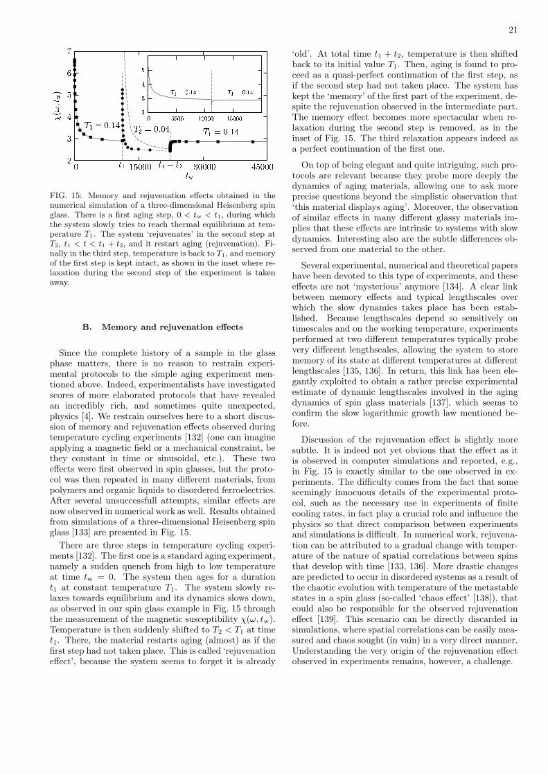
21

"! # $! %&'"!

(

)*+,-/.

0

!12 31

4

5

1

!2

6

FIG. 15: Memory and rejuvenation effects obtained in thenumerical simulation of a three-dimensional Heisenberg spinglass. There is a first aging step, 0 < tw < t1, during whichthe system slowly tries to reach thermal equilibrium at tem-perature T1. The system ‘rejuvenates’ in the second step atT2, t1 < t < t1 + t2, and it restart aging (rejuvenation). Fi-nally in the third step, temperature is back to T1, and memoryof the first step is kept intact, as shown in the inset where re-laxation during the second step of the experiment is takenaway.

B. Memory and rejuvenation effects

Since the complete history of a sample in the glassphase matters, there is no reason to restrain experi-mental protocols to the simple aging experiment men-tioned above. Indeed, experimentalists have investigatedscores of more elaborated protocols that have revealedan incredibly rich, and sometimes quite unexpected,physics [4]. We restrain ourselves here to a short discus-sion of memory and rejuvenation effects observed duringtemperature cycling experiments [132] (one can imagineapplying a magnetic field or a mechanical constraint, bethey constant in time or sinusoidal, etc.). These twoeffects were first observed in spin glasses, but the proto-col was then repeated in many different materials, frompolymers and organic liquids to disordered ferroelectrics.After several unsuccessfull attempts, similar effects arenow observed in numerical work as well. Results obtainedfrom simulations of a three-dimensional Heisenberg spinglass [133] are presented in Fig. 15.

There are three steps in temperature cycling experi-ments [132]. The first one is a standard aging experiment,namely a sudden quench from high to low temperatureat time tw = 0. The system then ages for a durationt1 at constant temperature T1. The system slowly re-laxes towards equilibrium and its dynamics slows down,as observed in our spin glass example in Fig. 15 throughthe measurement of the magnetic susceptibility χ(ω, tw).Temperature is then suddenly shifted to T2 < T1 at timet1. There, the material restarts aging (almost) as if thefirst step had not taken place. This is called ‘rejuvenationeffect’, because the system seems to forget it is already

‘old’. At total time t1 + t2, temperature is then shiftedback to its initial value T1. Then, aging is found to pro-ceed as a quasi-perfect continuation of the first step, asif the second step had not taken place. The system haskept the ‘memory’ of the first part of the experiment, de-spite the rejuvenation observed in the intermediate part.The memory effect becomes more spectacular when re-laxation during the second step is removed, as in theinset of Fig. 15. The third relaxation appears indeed asa perfect continuation of the first one.

On top of being elegant and quite intriguing, such pro-tocols are relevant because they probe more deeply thedynamics of aging materials, allowing one to ask moreprecise questions beyond the simplistic observation that‘this material displays aging’. Moreover, the observationof similar effects in many different glassy materials im-plies that these effects are intrinsic to systems with slowdynamics. Interesting also are the subtle differences ob-served from one material to the other.

Several experimental, numerical and theoretical papershave been devoted to this type of experiments, and theseeffects are not ‘mysterious’ anymore [134]. A clear linkbetween memory effects and typical lengthscales overwhich the slow dynamics takes place has been estab-lished. Because lengthscales depend so sensitively ontimescales and on the working temperature, experimentsperformed at two different temperatures typically probevery different lengthscales, allowing the system to storememory of its state at different temperatures at differentlengthscales [135, 136]. In return, this link has been ele-gantly exploited to obtain a rather precise experimentalestimate of dynamic lengthscales involved in the agingdynamics of spin glass materials [137], which seems toconfirm the slow logarithmic growth law mentioned be-fore.

Discussion of the rejuvenation effect is slightly moresubtle. It is indeed not yet obvious that the effect as itis observed in computer simulations and reported, e.g.,in Fig. 15 is exactly similar to the one observed in ex-periments. The difficulty comes from the fact that someseemingly innocuous details of the experimental proto-col, such as the necessary use in experiments of finitecooling rates, in fact play a crucial role and influence thephysics so that direct comparison between experimentsand simulations is difficult. In numerical work, rejuvena-tion can be attributed to a gradual change with temper-ature of the nature of spatial correlations between spinsthat develop with time [133, 136]. More drastic changesare predicted to occur in disordered systems as a result ofthe chaotic evolution with temperature of the metastablestates in a spin glass (so-called ‘chaos effect’ [138]), thatcould also be responsible for the observed rejuvenationeffect [139]. This scenario can be directly discarded insimulations, where spatial correlations can be easily mea-sured and chaos sought (in vain) in a very direct manner.Understanding the very origin of the rejuvenation effectobserved in experiments remains, however, a challenge.

22

C. Mean-field aging and effective temperatures

Theoretical studies of mean-field glassy models haveprovided important insights into the aging dynamics ofboth structural and spin glasses [140–142]. Althoughsuch models are defined in terms of spin degrees of free-dom interacting via infinite-ranged interactions, the deepconnections between them and the mode-coupling the-ory of the glass transition make them serious candi-dates to investigate glassy states in general, not onlythermodynamic properties at thermal equilibrium butalso non-equilibrium aging dynamics. Despite their of-ten reported ‘simplicity’, it took several years to derive aproper asymptotic solution of the long-time dynamics fora series of mean-field spin glasses [74]. These results havethen triggered an enormous activity [143] encompassingtheoretical, numerical and also experimental work try-ing to understand further these results, and to check inmore realistic systems whether they have some reason-able range of applicability beyond mean-field. This largeactivity, by itself, easily demonstrates the broad interestof these results.

In these mean-field models, thermal equilibrium isnever reached, and aging proceeds by downhill motionin an increasingly flat free energy landscape [144], withsubtle differences between spin glass and structural glassmodels. In both cases, however, time translational in-variance is broken, and two-time correlation and responsefunctions depend on both their time arguments. In fact,the exact dynamic solution of the equations of motionfor time correlators displays behaviours in strikingly goodagreement with the numerical results reported in Fig. 14.

In these systems, the equations of motion in the ag-ing regime involve not only time correlations, but alsotime-dependent response functions. At thermal equi-librium response and correlations are not independent,since the fluctuation-dissipation theorem (FDT) relatesboth quantities. In aging systems, there is no reason toexpect the FDT to hold and both quantities carry, atleast in principle, distinct physical information. Again,the asymptotic solution obtained for mean-field modelsquantitatively establishes that the FDT does not apply inthe aging regime. Unexpectedly, the solution also showsthat a generalized form of the FDT holds at large waitingtimes [140]. This is defined in terms of the two-time con-nected correlation function for some generic observableA(t),

C(t, tw) = 〈A(t)A(tw)〉 − 〈A(t)〉〈A(tw)〉, (27)

with t ≥ tw, and the corresponding two-time (impulse)response function

R(t, tw) = Tδ〈A(t)〉δh(tw)

∣

∣

∣

∣

∣

h=0

. (28)

Here h denotes the thermodynamically conjugate field tothe observable A so that the perturbation to the Hamil-tonian (or energy function) is δE = −hA, and angled

brackets indicate an average over initial conditions andany stochasticity in the dynamics. Note that we haveabsorbed the temperature T in the definition of the re-sponse, for convenience. The associated generalized FDTreads then

R(t, tw) = X(t, tw)∂

∂twC(t, tw), (29)

with X(t, tw) the so-called fluctuation-dissipation ratio(FDR). At equilibrium, correlation and response func-tions are time translation invariant, depending only onτ = t−tw, and equilibrium FDT imposes that X(t, tw) =1 at all times. A parametric fluctuation-dissipation (FD)plot of the step response or susceptibility

χ(t, tw) =

∫ t

tw

dt′ R(t, t′), (30)

against

∆C(t, tw) = C(t, t) − C(t, tw), (31)

is then a straight line with unit slope. These simplifi-cations do not occur in non-equilibrium systems. Butthe definition of an FDR through Eq. (29) becomes sig-nificant for aging systems [140, 141]. In mean-field spinglass models the dependence of the FDR on both timearguments is only through the correlation function,

X(t, tw) ∼ X(C(t, tw)), (32)

valid at large wait times, tw → ∞. For mean-field struc-tural glass models, the simplication (32) is even morespectacular since the FDR is shown to be characterizedby only two numbers instead of a function, namely X ∼ 1at short times (large value of the correlator) correspond-ing to a quasi-equilibrium regime, with a crossover to anon-trivial number, X ∼ X∞ for large times (small valueof the correlator). This implies that parametric FD plotsare simply made of two straight lines with slope 1 andX∞, instead of the single straight line of slope 1 obtainedat equilibrium.

Since any kind of behaviour is in principle allowedin non-equilibrium situations, getting such a simple,equilibrium-like structure for the FD relations is a re-markable result. This immediately led to the idea thataging systems might be characterized by an effective ther-modynamic behaviour and the idea of quasi-equilibrationat different timescales [145, 146]. In particular, general-ized FD relations suggest to define an effective tempera-ture, as

Teff =T

X(t, tw), (33)

such that mean-field glasses are characterized by a uniqueeffective temperature, Teff = T/X∞. It is thoughtof as the temperature at which slow modes are quasi-equilibrated. One finds in general that 0 < X∞ < 1,

23

such that Teff > T , as if the system had kept some mem-ory of its high temperature initial state.

The name ‘temperature’ for the quantity defined inEq. (33) is not simply the result of a dimensional anal-ysis but has a deeper, physically appealing meaningthat is revealed by asking the following questions. Howdoes one measure temperatures in a many-body sys-tem whose relaxation involves well-separated timescales?What is a thermometer (and a temperature) in a farfrom equilibrium aging material? Answers are providedin Refs. [145, 147] both for mean-field models and for ad-dditional toy models with multiple relaxation timescales.The idea is to couple an additional degree of freedom,such as a harmonic oscillator, x(t), which plays the role ofthe thermometer operating at frequency ω, to an observ-able of interest A(t) via a linear coupling, −λx(t)A(t).Simple calculations show then that the thermometer‘reads’ the following temperature,

1

2KBT

2meas ≡

1

2ω2〈x2〉 =

ωC ′(ω, tw)

2χ′′(ω, tw), (34)

where C ′(ω, tw) is the real part of the Fourier trans-form of Eq. (27), and χ(ω, tw) the imaginary part of theFourier transform of Eq. (28), with h = λx. The relation(34) indicates that the bath temperature is measured,Tmeas = T , if frequency is high and FDT is satisfied,while Tmeas = Teff > T if frequency is slow enough to betuned to that of the slow relaxation in the aging material.The link between the FDR in Eq. (29) and the effectivetemperature measured in Eq. (34) was numerically con-firmed in the computer simulation of a glassy molecularliquid in Ref. [148].

More generally, relaxation in glassy systems occurs inwell-separated time sectors [141]; it is then easy to imag-ine that each sector could be associated with an effec-tive temperature [147]. A thermodynamic interpretationof effective temperatures has also been put forward, re-lating them to the concept of replica symmetry break-ing [149]. Interestingly, the full-step or one-step replicasymmetry breaking schemes needed to solve the staticproblem in these models have a counterpart as the FDRbeing a function or a number, respectively, in the ag-ing regime. Moreover, we note that these modern con-cepts are related to, but make much more precise, olderideas of quasi-equilibrium and fictive temperatures in ag-ing glasses [3].

Taken together, these results make the mean-field de-scription of aging very appealing, and they nicely comple-ment the mode-coupling/RFOT description of the equi-librium glass transition described above. Moreover, theyhave set the agenda for a large body of numerical andexperimental work, as reviewed in [143]. In Fig. 16we present recent numerical data obtained in an agingsilica glass [150], presented in the form of a paramet-ric response-correlation plot. The measured correlationfunctions are the self-part of the intermediate scatter-ing functions defined in Eq. (5), while the conjugatedresponse functions quantify the response of particle dis-

4 × 1041 × 1042 × 103

t = 5 × 102FDT

O

Si

T = 2500 K

C(t, t′)

Tχ(t

,t′)

1.210.80.60.4

0.6

0.4

0.2

0

FIG. 16: Parametric correlation-response plots measured inthe aging regime of a numerical model for a silica glass,SiO2 [150]. The plots for both species smoothly convergestowards a two-straight line plot of slope 1 at short times(large C values), and of slope X∞

≈ 0.51 at large times(small values of C), yielding an effective temperature of aboutTeff = T/X∞

≈ 4900 K.

placements to a spatially modulated field conjugated tothe density. Plots for silicon and oxygen atoms at dif-ferent ages of the system are presented. They seem tosmoothly converge towards a two-straight line plot, asobtained in mean-field models. Moreover, the second,non-trivial part of the plot is characterized by a slopethat appears to be independent of the species, and of thewavevector chosen to quantity the dynamics, in agree-ment with the idea of a unique asymptotic value of theFDR, possibly related to a well-defined effective temper-ature.

D. Beyond mean-field

Despite successes such as shown in Fig. 16, the broaderapplicability of the mean-field scenario of aging dynamicsremains unclear, however. While some experiments andsimulations indeed seem to support the existence of well-behaved effective temperatures [151–153], other studiesalso reveal the limits of the mean-field scenario. Experi-ments have for instance reported anomalously large FDTviolations associated with intermittent dynamics [154–157], while theoretical studies of model systems havealso found non-monotonic or even negative response func-tions [158–161], and ill-defined or observable-dependentFDRs [162]. In principle, these discrepancies with mean-field predictions are to be expected, since there are manysystems of physical interest in which the dynamics arenot of mean-field type, displaying both activated pro-cesses and spatial heterogeneity.

It is thus an important task to understand from thetheoretical point of view when the mean-field conceptof an FDR-related effective temperature remains viable.However, studying theoretically the interplay betweenrelevant dynamic lengthscales and thermally activated

24

dynamics in the non-equilibrium regime of disorderedmaterials is clearly a challenging task. Nevertheless, thisproblem has been approached in different ways, as webriefly summarize in this subsection.

A first class of system that displays aging and spa-tial heterogeneity is given by coarsening systems. Theparadigmatic situation is that of an Ising ferromagneticmodel (with a transition at Tc) suddenly quenched inthe ferromagnetic phase at time tw = 0. For tw > 0domains of positive and negative magnetizations appearand slowly coarsen with time. The appearance of do-mains that grow with time proves the presence of bothaging and heterogeneity in this situation.

The case where the quench is performed down toT < Tc is well understood. The system becomes scaleinvariant [163], since the only relevant lengthscale is thegrowing domain size, `(tw). Correlation functions dis-play aging, and scale invariance implies that C(t, tw) ∼f(`(t)/`(tw)). Response functions can be decomposedinto two contributions [164, 165]: one part stems fromthe bulk of the domains and behaves as the equilibriumresponse, and a second one from the domain walls andbecomes vanishingly small in the long time limit where`(tw) → ∞ and the density of domain walls vanishes.This implies that for coarsening systems in d ≥ 2, onehas X∞ = 0, or equivalently an infinite effective tem-perature, Teff = ∞. The case d = 1 is special becauseTc = 0 and the response function remains dominatedby the domain walls, which yields the non-trivial valueX∞ = 1/2 [166].

Another special case has retained attention. When thequench is performed at T = Tc, there is no more dis-tinction between walls and domains and the above ar-gument yielding X∞ = 0 does not hold. Instead onestudies the growth with time of critical fluctuations, with

ξ(tw) ∼ t1/zw the correlation length at time tw, where z

is the dynamic exponent. Both correlation and responsefunctions become non-trivial at the critical point [167].It proves useful in that case to consider the dynamicsof the Fourier components of the magnetization fluctu-ations, Cq(t, tw) = 〈mq(t)m−q(tw)〉, and the conjugated

response Rq(t, tw) =δ〈mq(t)〉δh−q(tw) . From Eq. (29) a wavevec-

tor dependent FDR follows, Xq(t, tw), which has inter-esting properties [168, 169].

In dimension d = 1, it is possible to compute Xq(t, tw)exactly in the aging regime at T = Tc = 0. An inter-esting scaling form is found, and numerical simulationsperformed for d > 1 confirm its validity:

Xq(t, tw) = X (q2tw), (35)

where the scaling function X (x) is X (x → ∞) → 1 atsmall lengthscale, qξ 1, and X (x → 0) → 1/2 (ind = 1) at large distance, qξ 1; recall that for z = 2 inthat case.

Contrary to mean-field systems where geometry playedno role, here the presence of a growing correlation length-scale plays a crucial role in the off-equilibrium regime

!#"$ %'&%)(*+, "$ % &%*

-'. /-'. 0-'. 1-'.32-

-

4

4 2

4

FIG. 17: Parametric response-correlation plots for the Fouriercomponents of the mobility field in the d = 3 Fredrickson-Andersen model. Symbols are from simulations, lines fromanalytic calculations, and wavevectors decrease from top tobottom. The FDT is close to being satisfied at large q corre-sponding to local equilibrium. At larger distance deviationsfrom the FDT are seen, with an asymptotic FDR which be-comes negative. Finally, for energy fluctuations at q = 0(bottom curve), the plot becomes a pure straight line of (neg-ative!) slope -3, as a result of thermally activated dynamics.

since ξ(tw) allows one to discriminate between fluctua-tions that satisfy the FDT at small lengthscale, Xq ∼ 1,and those at large lenghtscale which are still far fromequilibrium, 0 < Xq ∼ X∞ < 1. These studies suggesttherefore that generalized fluctuation-dissipation relationin fact have a strong lengthscale dependence—a resultwhich is not predicted by mean-field approaches.

Another interesting result is that the FDT violationfor global observables (i.e. those at q = 0) takes a par-ticularly simple form, since the introduction of a sin-gle number is sufficient, the FDR at zero wavevector,Xq=0(t, tw) ≡ X∞ = 1/2 (in d = 1). This universalquantity takes non-trivial values in higher dimension, e.g.X∞ ≈ 0.34 is measured in d = 2 [168]. This shows thatthe study of global rather than local quantities makes themeasurement of X∞ much easier. Finally, having a non-trivial value of X∞ for global observables suggests thatthe possibility to define an effective temperature remainsvalid, but it has become a more complicated object, re-lated to global fluctuations on large lengthscale.

Kinetically constrained spin models represent a secondclass of non-mean-field systems whose off-equilibrium hasbeen thoroughly studied recently [104]. This is quite anatural thing to do since these systems have local, finiteranged interactions, and they combine the interesting fea-tures of being defined in terms of (effective) microscopicdegrees of freedom, having local dynamical rules, and dis-playing thermally activated and heterogeneous dynamics.

The case of the Fredrickson-Andersen model, describedin Sec. VII, has been studied in great detail [104], andwe summarize the main results. Here, the relevant dy-namic variables are the Fourier components of the mobil-ity field, which also correspond in that case to the fluc-

25

tuations of the energy density. Surprisingly, the struc-ture of the generalized fluctuation-dissipation relation re-mains once more very simple. In particular, in dimen-sion d > 2, one finds a scaling form similar to (35),Xq(t, tw) = X (q2tw), with a well-defined limit at largedistance Xq=0(t, tw) ≡ X∞. The deep analogy with crit-ical Ising models stems from the fact that mobility de-fects in KCMs diffuse in a way similar to domain walls incoarsening Ising models. It is in fact by exploiting thisanalogy that analytic results are obtained in the agingregime of the Fredrickson-Andersen model [170].

There is however a major qualitative difference be-tween the two families of model. The (big!) surpriselies in the sign of the asymptotic FDR, since calculationsshow that [171]

X∞ = −3, d > 2. (36)

In dimension d = 1, one finds Xq=0(t, tw) = f(t/tw) withXq=0(t → ∞, tw) = 3π

16−6π ≈ −3.307. Numerical simula-tions confirm these calculations. In Fig. 17, we show sucha comparison between simulations (symbols) and theory(lines) in the case of the d = 3 Fredrickson-Andersenmodel [171]. Fourier components of the mobility fieldyield parametric FD plots that follow scaling with thevariable q2tw, as a direct result of the presence of a grow-ing lengthscale for dynamic heterogeneity, ξ(tw) ∼ √

tw.Again, generalized fluctuation-dissipation relations ex-plicitely depend on the spatial lengthscale considered,unlike in mean-field studies. In Fig. 17, the limit q = 0corresponding to global observables is also very interest-ing since the plot is a pure straight line, as in equilibrium.Unlike equilibrium, however, the slope is not 1 but −3.A negative slope in this plot means a negative FDR, andtherefore suggests a negative effective temperature, anvery non-intuitive result at first sight.

Negative response functions in fact directly followsfrom the thermally activated nature of the dynamics ofthese models [171]. First, one should note that the globalobservable shown in Fig. 17 corresponds to fluctuationsof the energy, e(tw), whose conjugated field is tempera-ture. In the aging regime the system slowly drifts towardsequilibrium. Microscopic moves result from thermally ac-tivated processes, corresponding to the local crossing ofenergy barriers. An infinitesimal change in temperature,T → T + δT with δT > 0, accelerates these barrier cross-ings and makes the relaxation dynamics faster. The en-ergy response to a positive temperature pulse is thereforenegative, δe < 0, which directly yields δe/δT < 0, whichexplains the negative sign of the FDR. This result doesnot hold in mean-field glasses, where thermal activationplays no role.

Finally, another scenario holds for local observables insome KCMs when kinetic constraints are stronger, suchas the East model [104] or a bidimensional triangularplaquette model [172]. Here, relaxation is governed bya hierarchy of energy barriers that endow the systemswith specific dynamic properties. In the aging regimefollowing a quench, in particular, the hierarchy yields

an energy relaxation that arises in discrete steps whichtake place on very different timescales, reminiscent of the‘time sectors’ encountered in mean-field spin glasses. Sur-prisingly, it is found that to each of these discrete relax-ations one can associate a well-defined (positive) valueof the fluctuation-dissipation ratio, again reminiscent ofthe dynamics of mean-field spin glass models. Therefore,even in models that are very far from the mean-field limitthe physical picture of a slow relaxation taking place onmultiple timescales with each timescale characterized byan effective temperature seems to have some validity.

E. Driven glassy materials

We have introduced aging phenomena with the argu-ment that in a glass phase, the timescale to equilibratebecomes so long that the system always remembers itscomplete history. This is true in general, but one canwonder whether it is possible to invent a protocol wherethe material history could be erased, and the system‘rejuvenated’ [173]. This concept has been known fordecades in the field of polymer glasses, where complexthermo-mechanical histories are often used.

Let us consider an aging protocol where the system isquenched to low temperature at time tw = 0, but the sys-tem is simultaneously forced by an external mechanicalconstraint. Experimentally one finds that a stationarystate can be reached, which explicitely depends on thestrength of the forcing: a system which is forced morestrongly relaxes faster than a less solicited material, aphenomenon called ‘shear-thinning’. The material hastherefore entered a driven steady state, where memoryof its age is no longer present and dynamics has becomestationary: aging is stopped.

Many studies of these driven glassy states have beenperformed in recent years. In the language of the jam-ming phase diagram in Fig. 4, these correspond to stud-ies of the (Temperature, Load) plane for molecular liq-uids, or the (1/Density, Load) plane for colloidal systems.The former studies are relevant for the rheology of super-cooled liquids and glasses, and the T Tg limit corre-sponds to studies of the plasticity of amorphous solids,a broad field in itself. In the colloidal world, such stud-ies are also relevant for the newly-defined field of therheology of ‘soft glassy materials’. These materials are(somewhat tautologically) defined as those for which thenon-linear rheological behaviour is believed to result pre-cisely from the competition between intrinsically slow re-laxation processses and an external forcing [174]. It isbelieved that the rheology of dense colloidal suspensions,foams, emulsions, binary mixtures, or even biophysicalsystems are ruled by such a competition, quite a broadfield of application indeed.

From the point of view of statmech modeling, softglassy rheology can be naturally studied from the verysame angles as the glass transition itself. As such trapmodels [174, 175], mean-field spin glasses [81] and the re-

26

lated mode-coupling theory approach [82, 83] have beenexplicitely extended to include an external mechanicalforcing. In all these cases, one finds that a driven steadystate can be reached and aging is indeed expected to stopat a level that depends on the strength of the forcing.Many of the results obtained in aging systems about theproperties of an effective temperature are also shown toapply in the driven case, as shown both theoretically [81]and numerically [176]. A most interesting aspect is thatthe broad relaxation spectra predicted to occur in glassymaterials close to a glass transition directly translateinto ‘anomalous’ laws both for the linear rheological be-haviour (seen experimentally in the broad spectrum ofelastic, G′(ω), and loss, G′′(ω), moduli), and the non-linear rheological behaviour (a strong dependence of theviscosity η upon the shear rate γ).

IX. FUTURE DIRECTIONS

The problem of the glass transition, already very ex-citing in itself, has ramifications well beyond the physicsof supercooled liquids. Glassy systems figures among theeven larger class of ‘complex systems’. These are formedby a set of interacting degrees of freedom that show anemergent behaviour: as a whole they exhibit propertiesnot obvious from the properties of the individual parts.As a consequence the study of glass-formers as statisti-cal mechanics model characterized by frustrated inter-actions is a fertile ground to develop new concepts andtechniques that will likely be applied to other physical,and more generally, scientific situations.

An example, already cited in this review, are the re-cent progress obtained in computer science and informa-tion theory [5] using techniques originally developed forspin glasses and structural glasses. More progress is cer-tainly expected in the future along these interdisciplinaryroutes. Concerning physics, glassiness is such an ubiqui-tous and, yet as we showed, rather poorly understoodproblem that many developments are very likely to takeplace in the next decade.

Instead of guessing future developments of the field

(and then very likely be proven wrong!) we prefer to lista few problems we would like to see solved in the nextyears.

• Are the jamming transitions of granular media andcolloids related to the glass transition of super-cooled liquids? If yes, what is the common physicalmechanism behind the dramatic slowing down?

• Is the glass transition related to a true phase tran-sition? If yes, a static or a dynamic one? A finiteor zero temperature one?

• Do RFOT, defects models, or frustration-basedtheory form the correct starting points of ‘the’theory of the glass transition?

• What is the correct physical picture for the lowtemperature phase of glass-forming liquids and spinglasses?

• Are there general principles governing off-equilibrium equilibrium dynamics, and in particu-lar aging and sheared materials?

• Do non-disordered, finite-dimensional, finite-rangestatmech model exist that display a thermodynam-ically stable amorphous phase at low temperature?

Finally, notice that we did not discuss possible inter-plays between glassiness and quantum fluctuations. Thisis a very fascinating topic. Quantum glassiness, and moregenerally, slow quantum dynamics are research subjectswhich are still in their infancies but that will likely un-dergo exciting developments in the near future.

Acknowledgments

We thank C. Marchetti for inviting us to write thisreview and the collaborators who worked with us on glassphysics. Our work is supported by ANR Grants CHEF,TSANET and DYNHET.

[1] C. A. Angell, Science 267, 1924 (1995).[2] P.G. Debenedetti and F. H. Stillinger, Nature 410, 259

(2001).[3] L. C. E. Struik, Physical aging in amorphous polymers

and other materials (Elsevier, Amsterdam, 1978).[4] Spin glasses and random fields, Ed.: A. P. Young (World

Scientific, Singapore, 1998).[5] Complex systems, Eds.: M. Mezard, J.-P. Bouchaud,

and J. Dalibard (Springer, Berlin, 2007).[6] H. Bassler, Phys. Rev. Lett. 58, 767 (1987).[7] R. Richert and C. A. Angell, J. Chem. Phys. 108, 9016

(1998).[8] A. W. Kauzmann, Chem. Rev. 43, 219 (1948)

[9] M. Goldstein, J. Chem. Phys. 51, 3728 (1969)[10] P. G. Debenedetti, Metastable liquids (Princeton Uni-

versity Press, Princeton, 1996)[11] See however N. Menon and S. R. Nagel Phys. Rev. Lett.

74, 1230 (1995); L. A. Fernandez, V. Martin-Mayor, andP. Verrocchio Phys. Rev. E 73, 020501 (2006); Refs [96].

[12] J. Wuttke, W. Petry, and S. Pouget, J. Chem. Phys.105, 5177 (1996).

[13] K. Binder and W. Kob, Glassy materials and disordered

solids (World Scientific, Singapore, 2005).[14] L.C. Pardo, P. Lunkenheimer, A. Loidl, Phys. Rev. E

76, 030502(R) (2007).[15] R. G. Larson, The Structure and Rheology of Complex

27

Fluids (Oxford University Press, New York, 1999).[16] P. N. Pusey and W. van Megen, Nature 320, 340 (1986).[17] Z. Cheng, J., P. M. Chaikin, S. Phan, and W. B. Russel,

Phys. Rev. E 65, 041405 (2002).[18] W. K. Kegel and A. van Blaaderen, Science 287, 290

(2000).[19] E. Weeks, J. C. Crocker, A. C. Levitt, A. Schofield, and

D. A. Weitz, Science 287, 627 (2000).[20] L. Cipelletti, L. Ramos, Journal of Physics: Condensed

Matter 17 (2005) R253.[21] H. M. Jaeger, S. R. Nagel, and R. P. Behringer, Rev.

Mod. Phys. 68, 1259 (1996).[22] G. D’Anna, G. Gremaud, Nature 413, 407 (2001).[23] G. Marty and O. Dauchot, Phys. Rev. Lett. 94, 015701

(2005).[24] A. S. Keys, A. R. Abate, S. C. Glotzer, and D. J. Durian,

Nat. Phys.3, 260 (2007).[25] A. J. Liu and S. R. Nagel, Nature 396, 21 (1998).[26] F. Krzakala, A. Montanari, F. Ricci-Tersenghi, G. Se-

merjian, and L. Zdeborova, PNAS (2007) 104 10318.[27] E. Vidal Russell and N. E. Israeloff, Nature 408, 695

(2000).[28] A. N. Adhikari, N. A. Capurso, and D. Bingemann, J.

Chem. Phys. 127, 114508 (2007).[29] M. Allen and D. Tildesley, Computer Simulation of Liq-

uids (Oxford University Press, Oxford, 1987).[30] J. Horbach and W. Kob, Phys. Rev. E 64, 041503

(2001).[31] W. Gotze, J. Phys.: Condens. Matter 11, A1 (1999).[32] T. Gleim, W. Kob, and K. Binder, Phys. Rev. Lett. 81,

4404 (1998).[33] G. Szamel and E. Flenner, Europhys. Lett. 67, 779

(2004).[34] L. Berthier and W. Kob, J. Phys.: Condens. Matter 19,

205130 (2007).[35] L. Berthier, G. Biroli, J.-P. Bouchaud, W. Kob, K.

Miyazaki, and D. R. Reichman, J. Chem. Phys. 126,184503 (2007).

[36] L. Berthier, G. Biroli, J.-P. Bouchaud, W. Kob, K.Miyazaki, and D. R. Reichman, J. Chem. Phys. 126,184504 (2007).

[37] J. P. Garrahan, D. Chandler, Phys. Rev. Lett. 89,035704 (2002).

[38] M. M. Hurley and P. Harrowell, Phys. Rev. E. 52, 1694(1995).

[39] M. D. Ediger, Annu. Rev. Phys. Chem. 51, 99 (2000).[40] W. Kob, C. Donati, S. J. Plimpton, P. H. Poole, and S.

C. Glotzer, Phys. Rev. Lett. 79, 2827 (1997).[41] P. Chaudhuri, L. Berthier, and W. Kob, Phys. Rev.

Lett. 99, 060604 (2007).[42] J. P. Hansen and I. R. McDonald, Theory of Simple

Liquids (Academic, London, 1986).[43] M. K. Mapes, S. F. Swallen, and M. D. Ediger, J. Chem.

Phys. 124, 054710 (2006).[44] G. Tarjus and D. Kivelson, J. Chem. Phys. 103, 3071

(1995).[45] Y. Jung, J.P. Garrahan, and D. Chandler, Phys. Rev.

E 69, 061205 (2004).[46] U. Tracht, M. Wilhelm, A. Heuer, H. Feng, K. Schmidt-

Rohr, and H. W. Spiess, Phys. Rev. Lett. 81, 2727(1998); S. A. Reinsberg, X. H. Qiu, M. Wilhelm, H. W.Spiess, M. D. Ediger, J. Chem. Phys. 114, 7299 (2001).

[47] S. Franz and G. Parisi, J. Phys.: Condens. Matter 12,6335 (2000).

[48] C. Toninelli, M. Wyart, L. Berthier, G. Biroli, and J.-P.Bouchaud, Phys. Rev. E 71, 041505 (2005).

[49] R. Yamamoto and A. Onuki, Phys. Rev. E 58, 3515(1998).

[50] S. Franz, C. Donati, G. Parisi, and S. C. Glotzer, Philos.Mag. B 79, 1827 (1999).

[51] C. Bennemann, C. Donati, J. Baschnagel, and S. C.Glotzer, Nature 399, 246 (1999); N. Lacevic, F. W.Starr, T. B. Schroder, and S. C. Glotzer, J. Chem. Phys.119, 7372 (2003).

[52] L. Berthier, Phys. Rev. E 69, 020201(R) (2004).[53] M. Vogel and S. C. Glotzer, Phys. Rev. E 70, 061504

(2004).[54] L. Berthier, Phys. Rev. E 76, 011507 (2007).[55] O. Dauchot, G. Marty, and G. Biroli, Phys. Rev. Lett.

95, 265701 (2005).[56] E. R. Weeks, J. C. Crocker, and D. A. Weitz, J. Phys.:

Condens. Matter 19, 205131 (2007).[57] L. Berthier, G. Biroli, J.-P. Bouchaud, L. Cipelletti, D.

El Masri, D. L’Hote, F. Ladieu, and M. Pierno, Science310, 1797 (2005).

[58] C. Dalle-Ferrier, C. Thibierge, C. Alba-Simionesco, L.Berthier, G. Biroli, J.-P. Bouchaud, F. Ladieu, D.L’Hote, and G. Tarjus Phys. Rev. E 76, 041510 (2007).

[59] X. Y. Xia and P. G. Wolynes, Proc. Natl. Acad. Sci.U.S.A. 97, 2990 (2000).

[60] J. P. Garrahan and D. Chandler, Proc. Natl. Acad. ScU.S.A. 100, 9710 (2003).

[61] G. Tarjus, S. A. Kivelson, Z. Nussinov, and P. Viot, J.Phys.: Condens. Matter 17, R1143 (2005).

[62] C. Donati, J. Douglas, W. Kob, S. J. Plimpton, P. H.Poole, and S. C. Glotzer, Phys. Rev. Lett. 80, 2338(1998).

[63] G. A. Appignanesi, J. A. Rodriguez Fris, R. A. Montani,and W. Kob, Phys. Rev. Lett. 96, 057801 (2006).

[64] G. Adam and J. H. Gibbs, J. Chem. Phys. 43, 139(1958).

[65] M. Mezard, G. Parisi, and M. Virasoro, Spin Glass The-

ory and Beyond (World Scientific, Singapore, 1988).[66] T. R. Kirkpatrick and D. Thirumalai, Phys. Rev. Lett.

58, 2091 (1987); T. R. Kirkpatrick and P. G. Wolynes,Phys. Rev. A 35, 3072 (1987).

[67] G. Biroli and M. Mezard, Phys. Rev. Lett. 88, 025501(2001).

[68] D. R. Nelson, Defects and Geometry in Condensed Mat-

ter Physics (Cambridge University Press, Cambridge,2002).

[69] G. D. McCullagh, D. Cellai, A. Lawlor, and K. A. Daw-son, Phys. Rev. E 71, 030102 (20050.

[70] O. Rivoire, G. Biroli, O. C. Martin, M. Mezard, Eur.Phys. J. B 37, 55 (2004).

[71] D. J. Gross and M. Mezard, Nucl. Phys. B 240, 431(1984).

[72] R. Monasson, Phys. Rev. Lett. 75, 2847 (1995).[73] T. Castellani, A. Cavagna, Lecture notes of the school:

”Unifying Concepts in Glassy Physics III”, Bangalore,

June 2004, J. Stat. Mech. (2005) P05012[74] L. F. Cugliandolo in Ref. [75].[75] Slow relaxations and nonequilibrium dynamics in con-

densed matter, Eds: J.-L. Barrat, J. Dalibard, M. Feigel-man, J. Kurchan (Springer, Berlin, 2003).

[76] E. Leutheusser, Phys. Rev. A 29, 2765 (1984).[77] U. Bengtzelius, W. Gotze, A. Sjoilander, J. Phys. C 17,

5915 (1984).

28

[78] S. P. Das and G. F. Mazenko, Phys. Rev. A 34, 2265(1986).

[79] G. Biroli and J. P. Bouchaud, Europhys. Lett. 67, 21(2004).

[80] G. Biroli, J.-P. Bouchaud, K. Miyazaki, and D. R. Re-ichman, Phys. Rev. Lett. 97, 195701 (2006).

[81] L. Berthier, J.-L. Barrat, and J. Kurchan, Phys. Rev. E61, 5464 (2000).

[82] K. Miyazaki and D. R. Reichman, Phys. Rev. E. 66,050501(R) (2002).

[83] M. Fuchs and M. E. Cates, Phys. Rev. Lett. 89, 248304(2002).

[84] T. R. Kirkpatrick, D. Thirumalai, and P. G. Wolynes,Phys. Rev. A 40, 1045 (1989).

[85] J.-P. Bouchaud and G. Biroli, J. Chem. Phys. 121, 7347(2004).

[86] M. Dzero, J. Schmalian, and P. G. Wolynes, Phys. Rev.B 72, 100201 (2005).

[87] S. Franz, J. Stat. Mech. P04001 (2005); Europhys. Lett.73, 492 (2006);

[88] C. A. Angell, J. Res. NIST 102, 171 (1997).[89] I. Hodge, J. Res. NIST 102, 195 (1997).[90] G. P. Johari, J. Chem. Phys. 112, 8958 (2000).[91] M. Mezard and G. Parisi, Phys. Rev. Lett. 82, 747

(1999).[92] G. Parisi and F. Zamponi, J. Chem. Phys. 123, 144501

(2005).[93] F. Thalmann, J. Chem. Phys. 116, 3378 (2002).[94] B. Coluzzi and P. Verrocchio, J. Chem. Phys. 116, 3789

(2002).[95] M. Nauroth and W. Kob, Phys. Rev. E 55, 657 (1997).[96] A. Cavagna, T. S. Grigera, and P. Verrocchio, Phys.

Rev. Lett. 98, 187801 (2007).[97] W. Kob and H. C. Andersen, Phys. Rev. E 48, 4364

(1993).[98] F. Ritort and P. Sollich, Adv. Phys. 52, 219 (2003).[99] S. Franz, R. Mulet, and G. Parisi, Phys. Rev. E 65,

021506 (2002).[100] C. Toninelli, G. Biroli, and D. S. Fisher, Phys. Rev.

Lett. 92, 185504 (2004).[101] A. C. Pan, J. P. Garrahan, D. Chandler, Phys. Rev. E

72, 041106 (2005).[102] S. H. Glarum, J. Chem. Phys. 33, 639 (1960).[103] G. H. Fredrickson and H. C. Andersen, Phys. Rev. Lett.

53, 1244 (1984).[104] S. Leonard, P. Mayer, P. Sollich, L. Berthier, and J. P.

Garrahan, J. Stat. Mech. P07017 (2007).[105] M. H. Cohen and G. S. Grest, Phys. Rev. B 26, 6313

(1982).[106] G. H. Fredrickson and S. A. Brawer. J. Chem. Phys. 84,

3351 (1986).[107] S. Butler and P. Harrowell, J. Chem. Phys. 95, 4454

(1991); J. Chem. Phys. 95, 4466 (1991).[108] C. Toninelli, G. Biroli, and D. S. Fisher, Phys. Rev.

Lett. 96, 035702 (2006).[109] S. Whitelam, L. Berthier, and J.P. Garrahan, Phys.

Rev. E 71, 026128 (2005).[110] L. Berthier and J.P. Garrahan, J. Phys. Chem. B 109,

3578 (2005).[111] R. L. Jack, P. Mayer, and P. Sollich, J. Stat. Mech.:

Theory Exp. P03006 (2006).[112] L. Berthier, D. Chandler, and J.P. Garrahan, Europhys.

Lett. 69, 320 (2005).[113] D. Chandler, J. P. Garrahan, R. L. Jack, L. Maibaum

and A.C. Pan, Phys. Rev. E 74, 051501 (2006).[114] S. Whitelam, L. Berthier, and J. P. Garrahan, Phys.

Rev. Lett. 92, 185705 (2004).[115] M. T. Downton and M. P. Kennett, Phys. Rev. E 76,

031502 (2007).[116] J. P. Garrahan, J. Phys. Condens. Matter 14, 1571

(2002).[117] R. L. Jack, L. Berthier, and J. P. Garrahan, Phys. Rev.

E 72, 016103 (2005).[118] A.Lipowski, D.Johnston, D.Espriu, Phys.Rev.E 62,

3404 (2000).[119] J. P. Sethna, J. D. Shore, and M. Huang, Phys. Rev. B

44, 4943 (1991).[120] G. Biroli, J.-P. Bouchaud, and G. Tarjus, J. Chem.

Phys. 123, 044510 (2005).[121] M. Sellitto, G. Biroli, C. Toninelli Europhys. Lett. 69

496 (2005).[122] L. Berthier and J. P. Garrahan, J. Chem. Phys. 119,

4367 (2003).[123] S. Whitelam and J. P. Garrahan, J. Phys. Chem. B 108,

6611 (2004).[124] R. L. Jack and J. P. Garrahan, J. Chem. Phys. 123,

164508 (2005).[125] F. C. Franck, Proc. R. Soc. London 215, 43 (1952).[126] D. Kivelson, S. A. Kivelson, X.-L. Zhao, Z. Nussinov,

and G. Tarjus, Physica A 219, 27 (1995).[127] D. Coslovich and G. Pastore, J. Chem. Phys. 127,

124504 (2007).[128] J. P. Bouchaud, J. Phys. I France 2, 1705 (1992).[129] A. J. Bray and M.A. Moore, J. Phys. C 17, L463 (1984);

and in Heidelberg Colloquim on Glassy Dynamics, Eds.:J. L. van Hemmen and I. Morgenstern, Lectures Notesin Physics Vol. 275 (Springer, Berlin, 1987).

[130] D. S. Fisher and D. A. Huse, Phys. Rev. Lett. 56, 1601(1986).

[131] J. Kisker, L. Santen, M. Schreckenberg, and H. Rieger,Phys. Rev. B 53, 6418 (1996).

[132] P. Refregier, E. Vincent, J. Hammann, and M. Ocio, J.Phys. France 48, 1533 (1987).

[133] L. Berthier and A. P. Young, Phys. Rev. B 71, 214429(2005).

[134] L. Berthier, V. Viasnoff, O. White, V. Orlyanchik, andF. Krzakala, in Ref. [75]

[135] J.-P. Bouchaud, V. Dupuis, J. Hammann, and E. Vin-cent, Phys. Rev. B 65, 024439 (2001).

[136] L. Berthier and J.-P. Bouchaud, Phys. Rev. B 66,054404 (2002).

[137] F. Bert, V. Dupuis, E. Vincent, J. Hammann, and J.-P.Bouchaud, Phys. Rev. Lett. 92, 167203 (2004).

[138] A. J. Bray and M. A. Moore, Phys. Rev. Lett. 58, 57(1987).

[139] P. E. Jonsson, R. Mathieu, P. Nordblad, H. Yoshino,H. Aruga Katori, and A. Ito Phys. Rev. B 70, 174402(2004).

[140] L. F. Cugliandolo and J. Kurchan, Phys. Rev. Lett. 71,173 (1993).

[141] L. F. Cugliandolo and J. Kurchan. J. Phys. A 27, 5749(1994).

[142] S. Franz and M. Mezard, Europhys. Lett. 26 209 (1994).[143] A. Crisanti and F. Ritort, J. Phys. A 36 R181 (2003).[144] J. Kurchan and L. Laloux, J. Phys. A 29, 1929 (1996).[145] L. F. Cugliandolo, J. Kurchan, and L. Peliti, Phys. Rev.

E 55, 3898 (1997).[146] S. Franz, M.A. Virasoro J. Phys. A 33 (2000) 891.

29

[147] J. Kurchan, Nature 433, 222 (2005).[148] L. Berthier and J.-L. Barrat, Phys. Rev. Lett. 89,

095702 (2002).[149] S. Franz, M. Mezard, G. Parisi, and L. Peliti, Phys. Rev.

Lett. 81, 1758 (1998).[150] L. Berthier, Phys. Rev. Lett. 98, 220601 (2007).[151] T. S. Grigera and N. E. Israeloff, Phys. Rev. Lett. 83,

5038 (1999).[152] B. Abou and F. Gallet, Phys. Rev. Lett. 93, 160603

(2004).[153] P. Wang, C. M. Song, and H. A. Makse, Nat. Phys. 2,

526 (2006).[154] L. Bellon, S. Ciliberto, and C. Laroche, Europhys. Lett.

53, 511 (2001).[155] L. Bellon and S. Ciliberto, Physica D 168, 325 (2002).[156] L. Buisson, L. Bellon, and S. Ciliberto, J. Phys.: Con-

dens. Matter 15, S1163 (2003).[157] L. Buisson, S. Ciliberto, and A. Garcimartin, Europhys.

Lett. 63, 603 (2003).[158] P. Viot, J. Talbot, and G. Tarjus, Fractals 11, 185

(2003).[159] M. Nicodemi, Phys. Rev. Lett.82, 3734 (1999).[160] F. Krzakala, Phys. Rev. Lett. 94, 077204 (2005).[161] M. Depken and R. Stinchcombe, Phys. Rev. E 71,

065102 (2005).[162] S. Fielding and P. Sollich, Phys. Rev. Lett. 88, 050603

(2002).[163] A. J. Bray, Adv. Phys. 43, 357 (1994).[164] A. Barrat, Phys. Rev. E 57, 3629 (1998).[165] L. Berthier, J.-L. Barrat and J. Kurchan, Eur. Phys. J.

B 11, 635 (1999).[166] C. Godreche and J.-M. Luck, J. Phys. A 33, 1151

(2000); ‘ E. Lippiello and M. Zannetti, Phys. Rev. E61, 3369 (2000).

[167] C. Godreche and J.-M. Luck, J. Phys. A 33, 9141(2000).

[168] P. Mayer, L. Berthier, J.P. Garrahan, and P. Sollich,Phys. Rev. E 68, 016116 (2003)

[169] P. Calabrese and A. Gambassi, J. .Phys. A 38, R133(2005).

[170] P. Mayer and P. Sollich, J. Phys. A 40, 5823 (2007).[171] P. Mayer, S. Leonard, L. Berthier, J. P. Garrahan, and

P. Sollich, Phys. Rev. Lett. 96, 030602 (2006).

[172] R. L. Jack, L. Berthier, and J. P. Garrahan, J. Stat.Mech. P12005 (2006).

[173] G. B. McKenna and A. J. Kovacs, Polym. Eng. Sci. 24,1131 (1984).

[174] P. Sollich, F. Lequeux, P. Hebraud, and M. E. Cates,Phys. Rev. Lett. 78, 2020 (1997)

[175] P. Sollich, Phys. Rev. E 58, 738 (1998).[176] L. Berthier and J.-L. Barrat, J. Chem. Phys. 116, 6228

(2002).[177] The terminology ‘strong’ and ‘fragile’ is not related to

the mechanical properties of the glass but to the evo-lution of the short-range order close to Tg. Strong liq-uids, such as SiO2, have a locally tetrahedric structurewhich persists both below and above the glass transitioncontrary to fragile liquids whose short-range amorphousstructure disappears rapidly upon heating above Tg.

[178] The decrease at long times constitutes a major differ-ence with spin glasses. In a spin glass, χ4 would be amonotonically increasing function of time whose long-time limit coincides with the static spin glass suscepti-bility. Physically, the difference is that spin glasses de-velop long-range static amorphous order while structualglasses do not or, at least, in a different and more subtleway.

[179] In order to have a well-defined thermodynamics, Bethelattices are generated as random graphs with fixed con-nectivity, also called random regular graphs.

[180] There is of course no crystal state in disordered systemssuch as in Eq. (14). In the case of lattice glass models,there is a crystal phase but it can disappear dependingwhether the Bethe lattice is a Cayley tree or a randomregular graph.

[181] A critical (different) behaviour is expected and pre-dicted for models having a transition [108].

[182] This type of plaquette models, and other spin models,were introduced originally [118, 119] to show how ultra-slow glassy dynamics can emerge because of growingfree energy barriers.

[183] Most KCMs do not have a finite temperature dynami-cal transition and the ones displaying a transition havecritical properties different from MCT.