1 

 

                                                           

A Statistical Analysis of 10-pin Bowling Scores and an Examination of the Fairness of

Alternative Handicapping Systems1

Sarah Keogh and Donal O’Neill2

Abstract

Using data on approximately 1240 games of bowling we examine the statistical properties of

10-pin bowling scores. We find evidence that that the distribution of bowling scores is

approximately log-normally distributed with a common variance across players. This allows

us to consider the effectiveness of alternative handicapping systems in allowing less skilled

bowlers to compete against more skilled opponents. We show that the current system

mitigates against bowlers of low skill and propose a new system which we show works well

in equalising the playing field across all match-ups.

 1 We are grateful to Mark Hinchcliffe for providing us with the data used in this analysis and to Mark Delaney and Olive Sweetman for help comments on the paper.

2 Corresponding author: Economics Dept. NUI Maynooth, Ireland e:mail donal.oneill@nuim.ie

2 

 

I: Introduction

Primitive forms of bowling can be traced back as far as 3200BC (www.tenpinbowling.org

2011). Ten pin bowling as we know it, is thought to have originated from the German nine

pin bowling game called Kegal (www.tenpinbowling.org 2011). Today, it is estimated that

the sport of ten pin bowling is played by over 100 million people in more than 90 countries,

making it one of the most popular games played in the world.3 With this in mind, it’s

surprising how little quantitative analysis has been conducted on the sport.

Previous research has examined the correlation in scores between balls rolled Neal

(2004) using a binomial distribution while Dorsey-Palmateer and Smith (2004) used

empirical data to examine the phenomenon of a “hot-hand” whereby the probability of a

strike with a given ball depends on the score obtained with the previous ball. There has also

been a small body of work looking at the distribution of bowling scores (Cooper and

Kennedy (1990) and Hohn (2009)) that did not use observed data. The only paper we are

aware of that uses empirical data to analyse the distribution of bowling scores is work carried

out by Chen and Swartz (1994), which used data on five pin bowling scores, a less-popular

variant of ten-pin bowling played only in Canada. As noted by the authors however, their

results cannot be applied to ten pin bowling due to differences in rules, equipment and

scoring.

In this paper we carry out a statistical analysis of scores from approximately 1024

games of ten pin bowling to determine the distribution of these scores. Since the score of a

player in a single score is the sum over a number of frames one might expect something

approximating normality if a central limit theorem is in operation. We examine normality of

                                                            3 See World Tenpin Bowling Association website http://www.worldtenpinbowling.com/

3 

 

both the raw scores and a suitably chosen transformation of these scores. We then use the

results of this analysis to evaluate the effectiveness of alternative handicapping systems

currently used. The latter is very topical among elite bowlers because if a bowler believes a

certain handicapping system to be unfair towards them, they will not enter leagues or

competitions which use that system. Section II introduces the game of ten pin bowling and

describes the data set used in the analysis. The statistical analysis is conducted in section III,

while section IV compares current handicapping systems and proposes a new, alternative

system.

II: The Game and the Data Set

Ten pin bowling is a competitive sport in which a “bowler” rolls a bowling ball down the

lane with the aim of scoring points by knocking down as many pins as possible. Ten pin

bowling balls have a smooth surface bar two finger holes and a thumb hole. They have a

maximum diameter of 8.59 in., and range in weight from 6lb. to 16lb. The ball is rolled down

a wooden or synthetic lane with the objective of knocking down pins. The pins themselves

are 4.75 in. wide at their widest point and 15 in. tall. They weigh 3 lb., 6 oz. The bowling

lane itself is 60 ft. from the foul line to the centre of the headpin. Today it is estimated that

over 100 million bowlers play the sport in over 90 countries, making it one of the most

popular participant sport in the world.

A game of ten pin bowling consists of 10 frames. A bowler’s score is the sum of

points over the game. Frames 1 to 9 consist of a maximum of 2 legally delivered balls rolled

by the same bowler on the same lane. Frame 10 consists of a maximum of three legally

delivered balls by the same bowler on the same lane. In a frame of bowling, if a bowler

knocks down all ten pins with their first ball, then a strike is awarded. If all ten pins are

4 

 

                                                           

knocked down using two balls in any frame, a spare is awarded. A strike is worth 10 points,

plus the points received from the next two balls rolled. A spare is worth 10 points plus the

points received from the next ball rolled. A bowler who bowls a strike in the 10th frame is

awarded two extra balls, which allow the awarding of bonus points. A bowler who bowls a

spare in the 10th frame is awarded one additional ball to allow for the bonus points. The

maximum score in ten pin bowling is 300, and is achieved by having 12 strikes in a row in

one game. The typical average score for a woman is 153, and the typical average score for a

man is 173.4

The data set used in this paper was obtained from an adult ten pin bowling league in

Alsaa Bowling Centre, Dublin Airport, Ireland. The league is 18 weeks in duration. There are

23 bowlers in this league. These 23 bowlers played 3 games every Monday evening for the

18 weeks. This gives a maximum of 54 games per bowler with possibly some missing values.

This results in approximately 1240 games. Bowling scores vary in the data set. The maximum

score is 289, bowled by player 20, and the minimum score is 114 bowled by player 16. Skill

levels among the 23 bowlers differ. The average scores range from 153 (player 18) to 220

(player 7). Further summary statistics are given in Table 1.

III: Analysis

a. Raw Scores:

The first stage in this analysis will be to investigate if the raw data is approximately normally

distributed. To begin we construct kernel density estimates of the underlying density. Kernel

density estimation is a non-parametric way of estimating the probability density function of a

random variable (Sheather 2004). The kernel density estimates for each of the 23 bowlers are

 4 http://www.ten‐pinbowling.com/faq.htm#3 

given in Figure 1. In these figures a normal density with mean and variance derived from the

raw data is also provided for comparison. These graphs show deviations from normality for a

number of players For instance results for players 1, 2, 13 and 20 seem to be skewed to the

right, while players 5, 21 and 23 seem to have fatter tails that the underlying normal

distribution.

We supplement this graphical approach with a number of tests. The tests used are the

Shapiro-Francia test (Shapiro and Francia (1972), Royston (1983)) and the Skewness

Kurtosis test (D’Agostino et al (1990), Royston (1991)). The Shapiro-Francia test equals the

squared correlation between the ordered sample values and the expected order statistics of a

standard normal and thus measures the straightness of the normal probability plot of the

sample values. The Skewness Kurtosis test presents a test for normality based on skewness

and another based on kurtosis and then combines the two tests into an overall test statistic.

Each test is conducted for each player in the data set. Then the p values are combined using

Fisher’s Method (Fisher 1970). Fisher’s method combines p values for each test into one test

statistic using the formula:

where pi is the p value for the ith hypothesis test. When all the null hypotheses are true, and

the pi are independent, P has a chi-squared distribution with 2k degrees of freedom (Fisher

1925). The results for both tests are presented in Tables 2 and 3. For both tests we reject the

null hypothesis that all game scores are normally distributed.

b. Transformed Scores

5 

 

Having rejected normality of the raw scores we now consider whether it is possible to find a

transformation of the underlying scores which is well represented by a normal distribution.

To do this we consider Box-Transformations of the scores (Box and Cox 1964, Spitzer 1980).

The original form of the Box-Cox transformation, as appeared in their 1964 paper, takes the

following form:

10

0

( )

y

y

ln y

Formally we posit the existence of a λ such that bowling scores for player i in game j, yij, can

be written as :

( )ij i ijy

where єij is a draw from a normal distribution with mean zero and variance 2i . Under the

assumption of normality the density function for the jth observation of player i, can be written

1 222/ 2 2

ij i ij if exp / 2

The likelihood contribution for player i can then be written in terms of observed bowling

scores yij :

1*i ij

j

L f y ij

Where the last term is the Jacobian of the transformation from є to y. Taking logs we get

212 2

1 1

2 2 1i iT T

*i i i i ij i

j j

ln L c T / ln y ln y

ij

6 

 

where c is a constant. The log likelihood function across all players is then:

1

N* *

ii

ln L ln L

Since i is just the mean of ( )ijy , we can concentrate it out of the likelihood function by

replacing it with its maximum likelihood estimate

1

1

iT^

i i ij ij

T y y

We can simplify this further by solving for the parameter 2i directly from its first order

conditions in terms of the other parameters and the data. The maximum likelihood estimate of

2i is given by :

212

1

iT^

i i ij ij

T y y

Substituting this expression into the individual likelihood function we get a final concentrated

likelihood function depending only on and data.

2

1

1

2 1

i

i

T

ij i T~j*

i iji

y y

ln L c T / ln ln yT

ij

The concentrated log-likelihood across all players can then be written as

2

1

1 1

2 1

i

i

T

ij i TNj*

i ii ji

y y

ln L T / ln ln yT

j

7 

 

Maximising the concentrated likelihood function with respect to λ provides an estimated

value ^

=-.148 with a standard error of .199 (lnL=-3331.2102). Since we cannot reject =0

(i.e the log transformation) we adopt this for convenience throughout the remainder of the

paper.

Table 4 gives a brief description of the transformed log bowling scores. The kernel

density graphs for the transformed bowling scores of each of the 23 bowlers are given in

Figure 2 and the results of the formal tests are given in Tables 5 and 6. Looking at the

Shapiro-Francia test results in Table 5 we see that while individually normality is rejected for

2 out of the 23 players, Fisher’s combined test fails to reject the null-hypothesis of normality

across all players. Table 6 presents the results of the Skewness Kurtosis. At the player level

normality is rejected for only one of the twenty three players. Perhaps somewhat surprisingly

Fisher’s combined test for normality across all players is rejected, the result driven by one

single player. When this one player is omitted from the analysis the combined F-test fails to

reject normality across the remaining players.

Analysis of the handicapping system will require comparing scores of high and low

ability bowlers. To do this it is useful to first examine whether or not the variance of bowling

scores depends on a player’s ability. Figure 3 plots the variance of transformed scores against

average score for each of the twenty three players, as well as the predicted variances from a

least squares regression through the data.5 There is little evidence of a systematic relationship

between variability and average ability.6 The estimated slope coefficient of the linear

regression is -.002 with a robust standard error of .012.

                                                            5 The labels on each observation indicate the number of games played by the player in question.

6 In contrast the raw scores exhibit a significant positive relationship between ability and variability. This may reflect the dramatic impact of strikes and spares (most likely to be bowled by high ability bowlers) on scores in

8 

 

9 

 

                                                                                                                                                                                        

IV: Handicapping

In bowling leagues the range of abilities can be wide. In our sample the average scores

ranged from 155 to 220. In light of this a league may adopt a handicapping system. A

handicap is simply a number added to a player’s gross score after each game which is

dependent on the player’s average ability. Handicaps are used to allow less skilled bowlers

compete with highly skilled bowlers on a more equal playing field. The idea is the bowler

with the higher average should always have a smaller advantage given the handicapping

system. This provides an incentive for bowlers to improve their bowling scores. The

advantage of the higher average player should not be so great that it discourages the lower

average player. Formally the US Bowling Congress defines a handicap league as follows

“A handicap league is one in which handicap is added to a bowler’s score to place

bowlers and teams with varying degrees of skill on as equitable a basis as possible for

scheduled competition.” (USBC 2011)

However, they are not explicit as to what is meant by equitable. The Council of

National Golf unions, the association charged with determining the handicap scores for

golfers in Britain in Ireland, are more explicit in stating that “A golf handicap allows players

of all levels of golfing ability to compete against each other on a fair and equal basis.”7 Use

of the term equal suggests that the purpose of a handicap system is to equalise the probability

of victory across ability levels. It is this feature of the handicap system that we examine in the

context of 10-pin bowling.

 a given frame. This contrasts to other sports such as golf where there is some evidence that variability declines with ability (Bingham and Swartz (2000)).

7 http://www.congu.com/welcome.htm 

 

10 

 

There have been some studies of the fairness of handicapping system in other sports

(see McHale (2010) and Bingham and Swartz (2000) for examples in golf). However there

has been little empirical analysis on bowling handicaps. Chen and Swartz (1994) carried out a

statistical analysis of 5-pin bowling, a variant of bowling, which is played only in Canada.

However, the scoring in this version of the game differs significantly from the more popular

10-pin bowling version and little attention was paid to developing a more equitable

handicapping system.

There are several handicapping systems used in 10-pin bowling and they can vary

from league to league. When considering fairness in this context we need to consider both

players. It is important the handicapping system is fair to the lower average player in order to

provide an incentive to increase their bowling scores. However, we want to avoid systems

that are so generous such that the lower average bowler can win without playing very well;

the incentives from such a system are wrong for both players. Since the low ability player can

win without playing very well they have little incentive to improve their game. This in turn

may prohibit such players from competing in leagues that don’t use handicaps (scratch

leagues). On the other hand if the high ability player believes the system is such that they will

lose even when playing well, they will have little incentive to try hard and may opt out of

leagues using the system.

At present there are a variety of used in Ireland. Depending on which of the systems is

used the final score of a player with average ability mi (determined over previous games

played by the player) is adjusted by adding a bonus to their raw score. The bonus is

determined by a weighting factor (w) and a par or scratch score P as follows:

Bonus = w(P – mi)

The most common weighting factor is 80% or .8, though weighting factors as low as .66 are

used. Typical scratch scores are 220 or 200. Cleary the higher the weighting factor and par

score the more generous the system is. Typical handicap systems use w=.8 and P=220. Under

this system a player with an average of 120 would be credited with an extra 80 pins (or

equivalently have an extra 80 points added to their raw score) under this system. Reducing w

to .66 and P to 200 would result in the same player only receiving only an additional 52

points. Although the base or scratch score used to calculate the handicap affects the number

of pins added to a player’s score, the choice of base will not affect the probability of victory

provided the scores of both players are adjusted under the handicap. So for instance in cases

where negative handicaps are allowed (whereby players above the base score have pins

deducted from their gross score; “plus handicappers” in golfing terms) then only the

weighting factor will impact on the probability of victory.

With w=.8 and P=220 a bowler with an average of 160 would have to beat a lower

ability opponent with an average say of 120 by more than 32 (.8*40) points in order to win

the game. Letting the higher ability players score be denoted by X and that of the lower

ability player by Y, then to establish the probability that the favourite (high ability player)

wins, we need to determine Pr(X>Y+32). More generally we can think of variations in

handicap systems by considering Pr(X>Y+h) for a range of h (corresponding to different

handicap systems). Letting f(X,Y) denote the joint distribution of X and Y, we can write this

probability as :

0

x h

h

Pr X Y h f X ,Y dxdy

(1)

11 

 

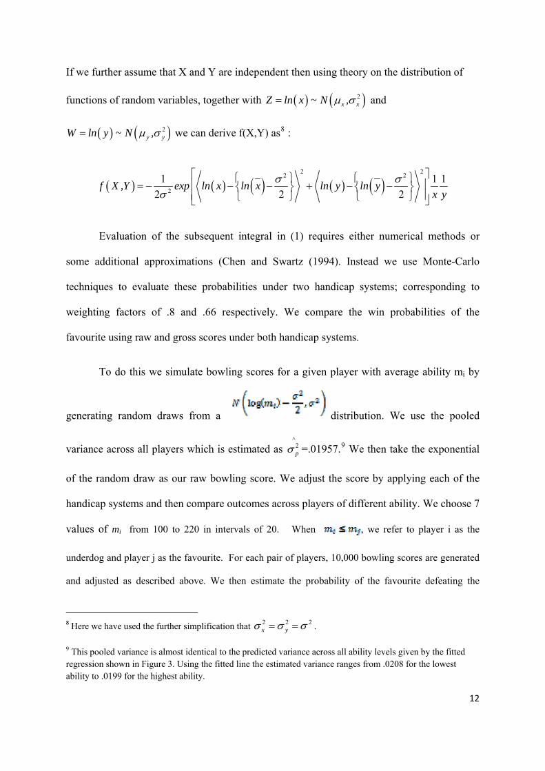
If we further assume that X and Y are independent then using theory on the distribution of

functions of random variables, together with 2x xZ ln x ~ N , and

2y yW ln y ~ N , we can derive f(X,Y) as8 :

2 2

2 2

2

1 1

2 2f X ,Y exp ln x ln x ln y ln y

1

2 x y

Evaluation of the subsequent integral in (1) requires either numerical methods or

some additional approximations (Chen and Swartz (1994). Instead we use Monte-Carlo

techniques to evaluate these probabilities under two handicap systems; corresponding to

weighting factors of .8 and .66 respectively. We compare the win probabilities of the

favourite using raw and gross scores under both handicap systems.

To do this we simulate bowling scores for a given player with average ability mi by

generating random draws from a distribution. We use the pooled

variance across all players which is estimated as 2^

p =.01957.9 We then take the exponential

of the random draw as our raw bowling score. We adjust the score by applying each of the

handicap systems and then compare outcomes across players of different ability. We choose 7

values of mi from 100 to 220 in intervals of 20. When , we refer to player i as the

underdog and player j as the favourite. For each pair of players, 10,000 bowling scores are generated

and adjusted as described above. We then estimate the probability of the favourite defeating the

                                                            2 2 2x y

12 

 

8 Here we have used the further simplification that . 

9 This pooled variance is almost identical to the predicted variance across all ability levels given by the fitted regression shown in Figure 3. Using the fitted line the estimated variance ranges from .0208 for the lowest ability to .0199 for the highest ability.

13 

 

underdog by computing the fraction of the 10,000 games the favourite has won based on raw and

adjusted scores.

Table 7 details the probabilities of the favourite winning across each possible match-

up using both raw unadjusted scores (first entry in each cell), adjusted according to most

generous system (2nd entry in each cell) and adjusted according to last generous system (3rd

entry in each cell). Looking first at the probabilities based on raw scores we see that even

with modest differences in ability the probability of the favourite winning is consistently over

75% and can quickly rise to above 90%. It is this imbalance in the probability of winning that

motivates the use of handicap systems. The 2nd and 3rd entry in each cell reports the

probability of the favourite winning using the scoring methods in the most generous and least

generous handicap systems. As expected the adjustment reduces the favourites advantage,

however the playing field remains far from level. The probability of a player with ability

level 180 beating a player with ability level 100 ranges from 70%-83% depending on the

system, despite the difference in skills having been taken into account in the handicap system.

It is clear from these results that even under the most generous handicap system currently

used in Irish bowling leagues the system remains inequitable with the more able players more

likely to win, especially when the ability differential is relatively large.

These simulated probabilities are based on our estimated variance and the assumption

of log normality. It is interesting to compare how these probabilities compare to the actual

outcomes in the bowling league under analysis. As well as the individual scores we also have

access to the average score of each player in the previous 20 games bowled (which is the

basis for the handicap score). For example at the start of the league player 7 had an average

of 220 and player 15 an average of 160. Since this was a team league these players never

competed directly against each other in head to head games. Nevertheless both players

14 

 

bowled in all 54 games, with their games taking place on the same evenings, at the same time

and in the same bowling alley. One check of our results is to compare the scores recorded by

both of these players on games played at the same time as if they were competing against

each other and to determine the victor in each of these 54 games. Using just the raw scores

we find that the high ability player would have emerged victorious in 53 of the 54 games. The

one exception was in game 49 when player 15 scored 189 compared to player 7’s score of

174. The higher ability player won all the remaining games with a margin of victory ranging

from 9 to 121 points. This comparison yields an estimated probability of victory for the high

ability player equal to .98, which compares favourably to our predicted estimate of .95. We

then repeat the analysis this time adjusting scores using a par score of 220 and a weighting

factor of .8 (similar to what is actually used in the league). With these adjusted scores the

number of games won by the favourite falls to 35, giving a probability of victory equal to

.648. This again compares very well to our simulated probability of .621. It would thus

appear that our simulated probabilities based on 10,000 simulated games provide estimates

that match very well to recorded victories, in actual league play based on much fewer games.

We now examine what changes, if any, to the handicap system would produce more

equitable outcomes. As noted earlier the key feature of handicap system determining the

probability of victory is the weighting factor. The United States Bowling Congress (2011)

recommends that their leagues adopt a weighting of 100% in order to equalise probabilities.

Table 8 shows the outcome probabilities under such a system. As expected this system

produces a much more level playing field with probabilities closer to .5. However, under this

scheme the odds of victory shift towards the lesser ability player. In all cases the probability

of the favourite wining is less than .5. Some authors (McHale 2010) argue that such a system

would distort incentives. Thus given the observed distribution of bowling scores in Ireland

15 

 

we would propose a weighting factor slightly less than 1. Table 9 shows the results obtained

when the weighting factor is .95. We see that across all match-ups the probability of the

favourite winning falls in the range .505-.547. This scheme thus results in a significant

levelling of the playing field without removing the incentive for players to improve their skill

level.

V: Conclusions

This paper examines the distribution of 10-pin bowling scores and uses the statistical results

to examine the impact of alternative handicapped scoring systems. We show that while the

raw bowling scores are not normally distributed, there is strong evidence that bowling scores

are normally distributed after a log-transformation. The simplicity of this transformation

helps when calculating the likelihood of victory in any match-up. Handicap scoring systems

are used in many bowling leagues with the explicit purpose of allowing players to compete

on a level playing field with players of lesser or greater skill. We use our results to examine

the performance of currently used handicap systems in Ireland. We show that the current

systems still leave large biases in favour of high ability players. Using a 100% weighting

factor produces a more level playing field but goes too far in the sense that players have no

incentive to improve their handicap. We propose a compromise weighting factor equal to .95

and shows that this system allows lower ability players to compete across all match-ups yet

still provides some incentives for players to improve their game.

16 

 

References

Bingham, D. and T. Swartz (2000), “Equitable Handicapping in Golf,” The American Statistician, Vol. 54, no. 3, pp. 170-177.

Box, G. E. P., and Cox, D. R. (1964), “An analysis of Transformations”, Journal of the Royal Statistical Society, 26, 211-243.

Chen, W. And Swartz, T. (1994), “Quantitative Aspects of Five-Pin Bowling”, The American Statistician, 48, 92-98.

Cooper, C. N. and Kennedy, R. (1990), “A Generating Function for the Distribution of the scores of all possible Bowling Games”, Mathematical Magazine, 63, 239-243.

D’Agostino, R. B., Belanger, A. and D’Agostino Jr. R. B. (1990), “A Suggestion for Using Powerful and Informative Tests of Normality, The American Statistician, 44, 316-321.

Dorsey-Palmeteer, R. And Smith, G. (2004), “Bowler’s Hot Hand”, The American Statistician, 58, 38-45.

Fisher, R.A. (1970), Statistical Methods for Research Workers 14th edition Hafner Publishing Company, New York

Hohn, J. L. (2009), “Generalized Probabilistic Bowling Distributions”, Unpublished Master’s Thesis, Western Kentucky University, Dept. of Mathematics.

McHale, I (2010), “Assessing the Fairness of the golf Handicap System in the UK,” Journal of Sports Sciences, 28(10), pp. 1033-1041.

Neal, D. K. (2004), “Random Bowling”, The Journal of Recreational Mathematics, 32, 125-129.

Royston, J. P. (1983), “A simple method for Evaluating the Shapiro-Francia W’ Test of Non-Normality”, Statistician, 32, 297-300.

Royston, J. P. (1991), “Comment on sg3.4 and an Improved D’Agostino Test”, Stata Technical Bulletin, 3, 13-24.

Shapiro, S. S. And Francia, R. S. (1972), “An Approximate Analysis of Variance Test for Normality”, Journal of the American Statistical Association, 67, 215-216.

Spitzer, J. J. (1982), “A Primer on Box-Cox Estimation”, The Review of Economics and Statistics, 64 (2), 307-313.

United States Bowling Congress (2011) USBC Playing Rules and commonly Asked Questions http://usbcongress.http.internapcdn.net/usbcongress/bowl/rules/pdfs/2011-2012PlayingRules.pdf

Figure 1: Kernel density of raw bowling scores for each player

 

 

 

 

17 

 

 

Figure 1 (continued)

 

 

 

18 

 

 

Figure 2: Kernel density of log transformed bowling scores for each player

 

 

19 

 

 

Figure 2: Continued

 

 

 

20 

 

 

Figure 3: Variance of log transformed bowling scores and average bowling score 

51 5138

41

34

10

5454

54

54

54

54

45

33

54

54 54

54

54

54

33

23

29

.01

.01

5.0

2.0

25

.03

.03

5

5 5.1 5.2 5.3 5.4average

variance Fitted values

 

21 

 

 

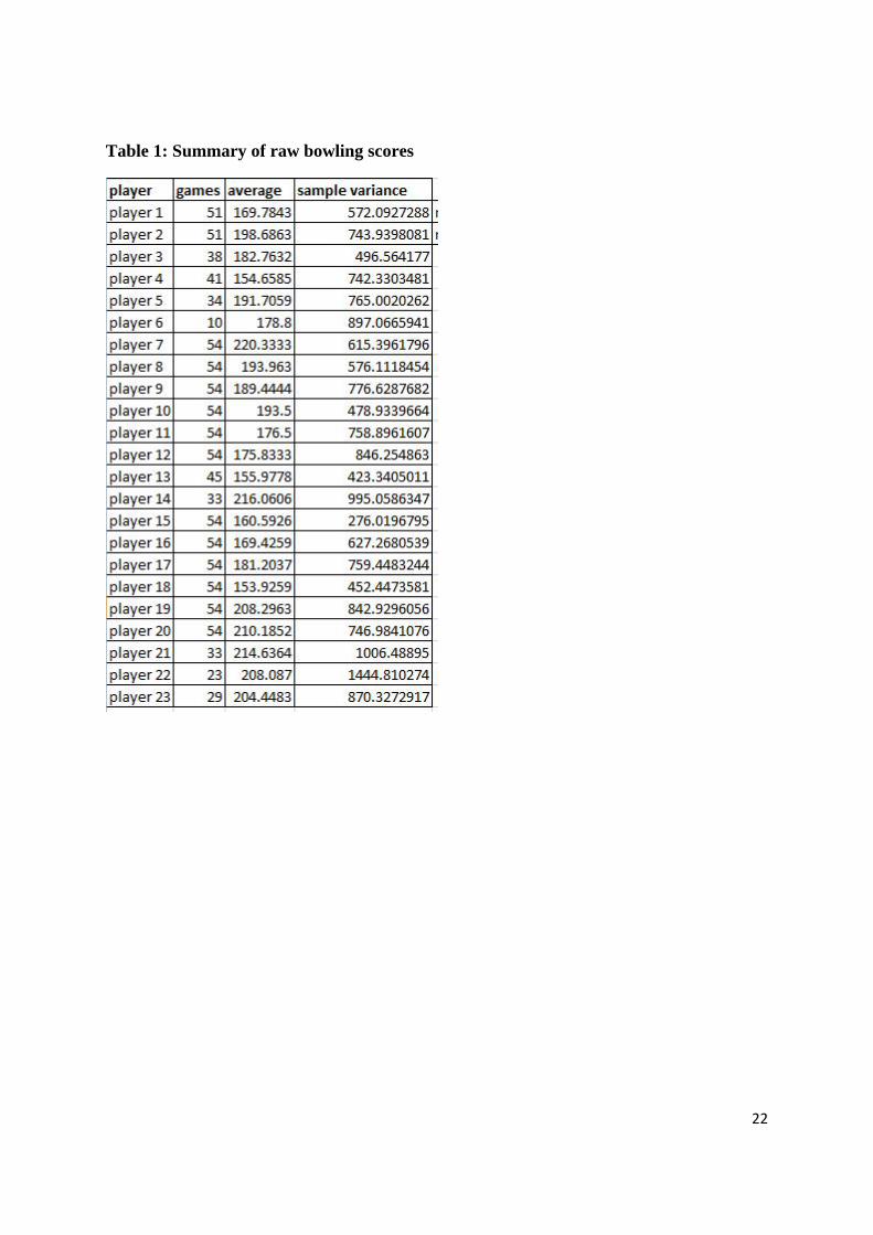
Table 1: Summary of raw bowling scores

 

22 

 

Table 2: Shapiro Francia Normality Test on the Raw Data

 

23 

 

Table 3: Skewness Kurtosis Normality Test on the Raw Data

 

24 

 

Table 4: Summary Statistics of Transformed Bowling Scores

 

25 

 

Table 5: Shapiro-Francia Test on Transformed Bowling Scores

 

26 

 

Table 6: Skewness Kurtosis Test on Transformed Bowling Scores

 

27 

 

28 

 

Table 7: Probabilities of favourite winning unadjusted scores and adjusted scores under handicap systems 1 and 6

Ability 100 120 140 160 180 200 220

100 .8184

.5665

.6178

.9527

.617

.7059

.9904

.661

.7672

.9985

.6981

.827

.9998

.7332

.8680

1

.7566

.8913

120 8184

.5665

.6178

.7775

.5604

.6036

.9236

.5963

.6761

.9812

.6411

.7394

.9962

.6800

.7944

.9989

.7035

.8332

140 .9527

.617

.7059

.7775

.5604

.6036

.7430

.5461

.5835

.8959

.5920

.6567

.9628

.6308

.7239

.9882

.6579

.7683

160 .9904

.661

.7672

.9236

.5963

.6761

.7430

.5461

.5835

.7299

.5457

.5808

.8722

.5845

.6462

.9514

.6207

.7033

180 9985

.6981

.827

.9812

.6411

.7394

.8959

.5920

.6567

.7299

.5457

.5808

.7063

.5419

.5754

.8503

.5797

.6346

200 .9998

.7332

.8680

.9962

.6800

.7944

.9628

.6308

.7239

.8722

.5845

.6462

.7063

.5419

.5754

.6848

.5348

.5633

220 1

.7566

.8913

.9989

.7035

.8332

.9882

.6579

.7683

.9514

.6207

.7033

.8503

.5797

.6346

.6848

.5348

.5633

29 

 

Table 8: Probabilities of favourite winning unadjusted and New handicap system based on 100% factor weighting

Ability 100 120 140 160 180 200 220

100 .8184

.4958

.9527

.4841

.9904

.4773

.9985

.4772

.9998

.4805

1

.4747

120 .8184

.4958

.7775

.4984

9236

.4838

.9812

.4806

.9962

.4833

.9989

.4775

140 .9527

.4841

.7775

.4984

.7430

.4918

.8959

.4891

.9628

.4908

.9882

.4836

160 .9904

.4773

.9236

.4838

.7430

.4918

.7299

.4934

.8722

.4963

.9514

.4907

180 .9985

.4772

.9812

.4806

.8959

.4891

.7299

.4934

.7063

.4973

.8503

.4949

200 .9998

.4805

.9962

.4833

.9628

.4908

.8722

.4963

.7063

.4973

.6848

.4952

220 1

.4747

.9989

.4775

.9882

.4836

.9514

.4907

.8503

.4949

.6848

.4952

Table 9: Probabilities of favourite winning unadjusted and New handicap system based on 95% weighting factor “Adjusted score = rawscoreplayer+.95(220-mi)”

Ability 100 120 140 160 180 200 220

100 .8184

.5155

.9527

.5184

.9904

.5264

.9985

.5330

.9998

.5465

1

.5472

120 .8184

.5155

.7775

.5152

.9236

.5133

.9812

.5196

.9962

.5311

.9989

.5353

140 .9527

.5184

.7775

.5152

.7430

.5039

.8959

.5137

.9628

.5291

.9882

.5268

160 .9904

.5264

.9236

.5133

.7430

.5039

.7299

.5057

.8722

.5187

.9514

.5243

180 .9985

.5330

.9812

.5196

.8959

.5137

.7299

.5057

.7063

.5080

.8503

.5186

200 .9998

.5465

.9962

.5311

.9628

.5291

.8722

.5187

.7063

.5080

.6848

.5050

220 1

.5472

.9989

.5353

.9882

.5268

.9514

.5243

.8503

.5186

.6848

.5050