A Stability and Performance of Various Singular Value QR ...

A

Stability and Performance of Various Singular Value QRImplementations on Multicore CPU with a GPU

Ichitaro Yamazaki, Stanimire Tomov, and Jack Dongarra,Department of Electrical Engineering and Computer Science,University of Tennessee, Knoxville, U.S.A.

Singular Value QR (SVQR) can orthonormalize a set of dense vectors with the minimum communication(one global reduction between the parallel processing units, and BLAS-3 to perform most of its local com-putation). As a result, compared to other orthogonalization schemes, SVQR obtains superior performanceon many of the current computers, where the communication has become significantly more expensive com-pared to the arithmetic operations. In this paper, we study the stability and performance of various SVQRimplementations on multicore CPUs with a GPU. Our focus is on the dense triangular solve, which per-forms half of the total floating-point operations of SVQR. As a part of this study, we examine an adaptivemixed-precision variant of SVQR, which decides if a lower-precision arithmetic can be used for the triangu-lar solution at run time without increasing the order of its orthogonality error (though its backward erroris significantly greater). If the greater backward-error can be tolerated, then our performance results withan NVIDIA Kepler GPU show that the mixed-precision SVQR can obtain a speedup of up to 1.36 over thestandard SVQR.

Categories and Subject Descriptors: G.1.0 [Mathematics of computing]: Numerical Analysis.

General Terms: Algorithms, Reliability, Performance.

Additional Key Words and Phrases: Orthogonalization; GPU computation; Mixed precision.

1. INTRODUCTIONOrthogonalizing a set of dense column vectors plays a salient part in many scientificand engineering computations. For example, it is a critical component in a softwarepackage that solves a large-scale linear system of equations or eigenvalue problem,having great impacts on both its numerical stability and performance. In many ofthese solvers, the input matrix to be orthogonalized is tall-skinny, having more rowsthan the columns. This is true, for instance, in a subspace projection method that com-putes the orthonormal basis vectors of the generated projection subspace [Saad 2003;Saad 2011]. Other applications of the tall-skinny orthogonalization include the solu-tion of an overdetermined least-squares problem [Golub and van Loan 2012]. Hence,an efficient and stable tall-skinny orthogonalization scheme is valuable in many appli-cations, especially if the scheme is suited for current and emerging computer architec-tures.

On the current computers, communication has become significantly more expensivecompared to arithmetic operations, where the communication includes data move-ment or synchronization between parallel processing units, as well as data movement

Authors’ address: Innovative Computing Laboratory, University of Tennessee, Department of Electrical En-gineering and Computer Science, Suite 203 Claxton 1122 Volunteer Boulevard, Knoxville, TN 37996. Au-thors’ emails: {iyamazak, tomov, dongarra}@eecs.utk.edu.Permission to make digital or hard copies of part or all of this work for personal or classroom use is grantedwithout fee provided that copies are not made or distributed for profit or commercial advantage and thatcopies show this notice on the first page or initial screen of a display along with the full citation. Copyrightsfor components of this work owned by others than ACM must be honored. Abstracting with credit is per-mitted. To copy otherwise, to republish, to post on servers, to redistribute to lists, or to use any componentof this work in other works requires prior specific permission and/or a fee. Permissions may be requestedfrom Publications Dept., ACM, Inc., 2 Penn Plaza, Suite 701, New York, NY 10121-0701 USA, fax +1 (212)869-0481, or [email protected]© YYYY ACM 0098-3500/YYYY/01-ARTA $15.00DOI:http://dx.doi.org/10.1145/0000000.0000000

ACM Transactions on Mathematical Software, Vol. V, No. N, Article A, Publication date: January YYYY.

A:2 I. Yamazaki et al.

between the levels of the local memory hierarchy. This holds in terms of both timeand energy consumptions. It is critical to take this hardware trend into considerationwhen designing high-performance software. To orthogonalize a tall-skinny dense ma-trix, both Cholesky QR (CholQR) and Singular Value QR (SVQR) [Stathopoulos andWu 2002] require only one global reduction between the parallel processing units, andperform most of their local computation using BLAS-3. Hence, compared to other or-thogonalization schemes, they obtain superior performance on the current computers.In addition, though the error bound of CholQR or SVQR depends quadratically on thecondition number of the input matrix, with a careful implementation and recursiveapplication of the procedure, CholQR and SVQR can stably orthogonalize many of theill-conditioned matrices in practice [Yamazaki et al. 2015]. As a result, we found thatCholQR is effective in many practical cases [Yamazaki et al. 2014; Yamazaki et al.2015; Yamazaki et al. 2014; Yamazaki et al. 2015].

Unfortunately, for some ill-conditioned matrices, CholQR may require many re-orthogonalizations (see Section 5). In this paper, we focus on SVQR which avoids thisnumerical difficulty of CholQR and has three advantages over CholQR in our currentcontext; First, the upper-bound on the orthogonality error of CholQR assumes that thesquared condition number of the input matrix is less than the reciprocal of the machineprecision, while the upper-bound of SVQR does not require this assumption; Second,for an ill-conditioned matrix, SVQR may be able to quickly identify the ill-conditionedsubspace, while CholQR may require multiple reorthogonalizations; Third, SVQR com-putes the condition number of the Gram matrix, which may be used to adapt the or-thogonalization scheme at run time.

We study the various implementations of SVQR on multicore CPUs with multipleGPUs. Though BLAS-3 kernels are used to performs most of the required flops ofSVQR, they must be carefully implemented to obtain stable and high performance.In this paper, we focus on the dense triangular solve, which performs half of the to-tal floating-point operations (flops) of SVQR.1 On a modern computer, lower-precisionarithmetic obtains higher peak-performance. To take advantage of this hardwaretrend, as a part of the current study, we examine an adaptive mixed-precision schemeto improve the performance of SVQR. Our adaptive scheme uses the orthogonality er-ror bound derived in [Yamazaki et al. 2015] and the computed condition number ofthe Gram matrix to adaptively decide if the lower precision can be used for the trian-gular solution without increasing its orthogonality error bound. The main trade-off isthat the backward-error of the mixed-precision SVQR is much greater. If the greaterbackward-error can be tolerated2, then our performance results with an NVIDIA Ke-pler GPU show that the mixed-precision SVQR can obtain a speedup of up to 1.36 overthe standard SVQR.

The rest of the paper is organized as follows: First, in Section 2, we present our im-plementation of CholQR and SVQR on multicore CPUs with multiple GPUs, and dis-cuss the numerical stability of these two algorithms in practice. Then, in Section 3, wepresent two different dense triangular solvers: one based on forward substitution andthe other based on matrix inversion. To overcome the potential numerical instabilityassociated with the matrix inversion, our implementation adaptively adjusts the sizesof the diagonal blocks to be inverted. Our implementation of the triangular solvers on aGPU and their performance are shown in Section 4. Finally, in Section 5, we introducethe adaptive mixed-precision SVQR, and in Sections 6 and 7, we show the numerical

1The symmetric matrix-matrix multiplication, which performs the other half of the total flops, is studiedin [Yamazaki et al. 2015].2Our preliminary studies indicated that in some cases, the greater backward error of the mixed-precisionSVQR may not significantly affect the solution convergence of some subspace projection methods.


Singular Value QR Implementations on Multicore CPUs with a GPU A:3

Step 1: Form Gram matrix B on GPUsfor p = 1, 2, . . . , np doB(p) := V (p)TV (p) on p-th GPU

end forB :=

∑np

p=1B(p) (GPUs to CPU global reduction)

Step 2: Compute upper-triangular matrix R on CPUwith CholQR with SVQRR := chol(B) [U,Σ, U ] = svd(B)

[W,R] := qr(√

ΣUT )

Step 3: Compute orthonormal matrix Q on GPUscopy R to all the GPUs (CPU to local GPUs broadcast)for p = 1, 2, . . . , np doQ(p) := V (p)R−1 on p-th GPU

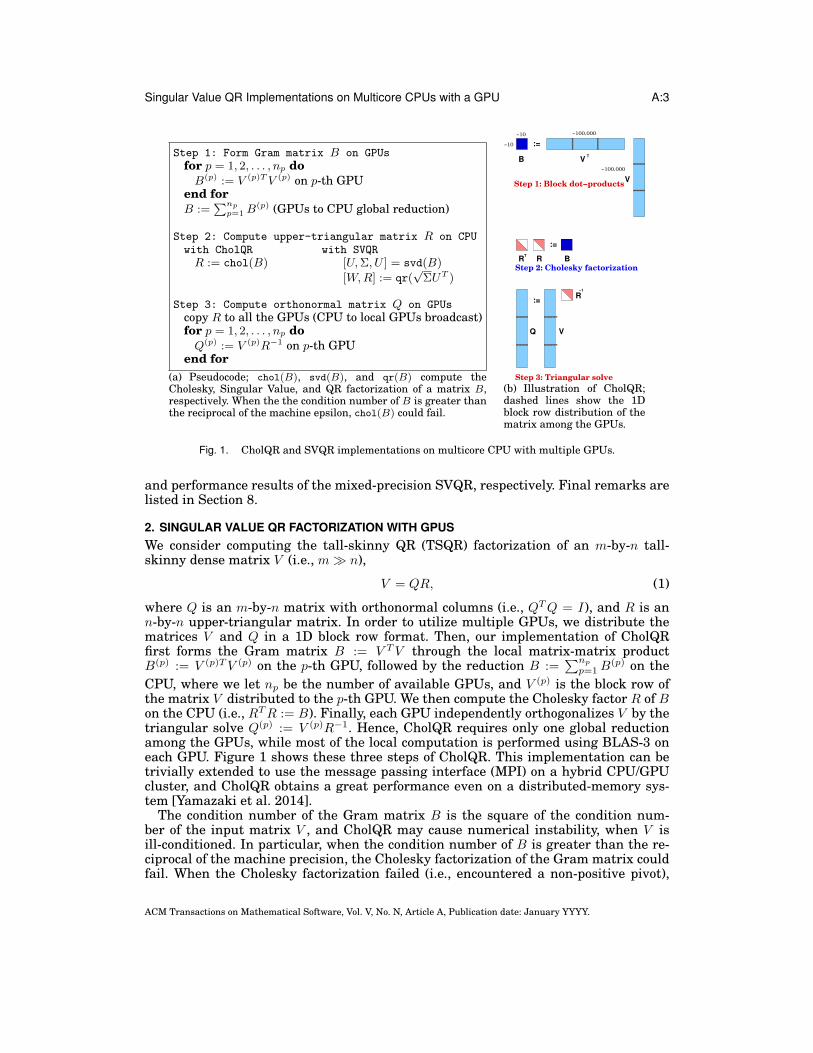
end for(a) Pseudocode; chol(B), svd(B), and qr(B) compute theCholesky, Singular Value, and QR factorization of a matrix B,respectively. When the the condition number of B is greater thanthe reciprocal of the machine epsilon, chol(B) could fail.

V

:=

B VT

Step 1: Block dot−products

:=

RT

R B

Step 2: Cholesky factorization

Q

:=

V

R−1

Step 3: Triangular solve

~100,000

~100,000~10

~10

(b) Illustration of CholQR;dashed lines show the 1Dblock row distribution of thematrix among the GPUs.

Fig. 1. CholQR and SVQR implementations on multicore CPU with multiple GPUs.

and performance results of the mixed-precision SVQR, respectively. Final remarks arelisted in Section 8.

2. SINGULAR VALUE QR FACTORIZATION WITH GPUSWe consider computing the tall-skinny QR (TSQR) factorization of an m-by-n tall-skinny dense matrix V (i.e., m� n),

V = QR, (1)

where Q is an m-by-n matrix with orthonormal columns (i.e., QTQ = I), and R is ann-by-n upper-triangular matrix. In order to utilize multiple GPUs, we distribute thematrices V and Q in a 1D block row format. Then, our implementation of CholQRfirst forms the Gram matrix B := V TV through the local matrix-matrix productB(p) := V (p)TV (p) on the p-th GPU, followed by the reduction B :=

∑np

p=1B(p) on the

CPU, where we let np be the number of available GPUs, and V (p) is the block row ofthe matrix V distributed to the p-th GPU. We then compute the Cholesky factor R of Bon the CPU (i.e., RTR := B). Finally, each GPU independently orthogonalizes V by thetriangular solve Q(p) := V (p)R−1. Hence, CholQR requires only one global reductionamong the GPUs, while most of the local computation is performed using BLAS-3 oneach GPU. Figure 1 shows these three steps of CholQR. This implementation can betrivially extended to use the message passing interface (MPI) on a hybrid CPU/GPUcluster, and CholQR obtains a great performance even on a distributed-memory sys-tem [Yamazaki et al. 2014].

The condition number of the Gram matrix B is the square of the condition num-ber of the input matrix V , and CholQR may cause numerical instability, when V isill-conditioned. In particular, when the condition number of B is greater than the re-ciprocal of the machine precision, the Cholesky factorization of the Gram matrix couldfail. When the Cholesky factorization failed (i.e., encountered a non-positive pivot),



‖A−QR‖2 ‖I −QTQ‖2 κ (Q)Iter. CholQR SVQR CholQR SVQR CholQR SVQR0 6.2× 101 6.2× 101 3.9× 103 3.9× 103 4.8× 1016 4.8× 1016

1 1.6× 10−15 (f) 3.5× 10−15 (t) 5.8× 102 (f) 1.0× 100 (t) 1.4× 1016 (f) 6.8× 108 (t)2 3.5× 10−15 (f) 5.6× 10−15 2.8× 102 (f) 6.7× 10−13 7.1× 1015 (f) 1.0× 100

3 3.9× 10−15 (f) 7.8× 10−15 1.9× 102 (f) 5.9× 10−15 6.6× 1015 (f) 1.0× 100

4 4.2× 10−15 1.2× 10−14 1.5× 102 3.0× 10−15 5.4× 1015 1.0× 100

5 4.4× 10−15 1.1× 10−14 1.0× 100 2.8× 10−15 2.3× 107 1.0× 100

6 4.4× 10−15 1.2× 10−14 4.7× 10−16 2.1× 10−15 1.0× 100 1.0× 100

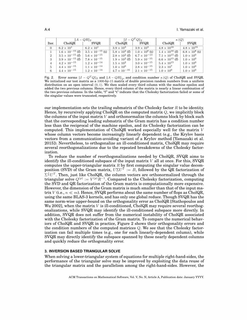
Fig. 2. Error norms ‖I − QTQ‖2 and ‖A−QR‖2, and condition number κ (Q) of CholQR and SVQR.We initialized our test matrix as a 1000-by-15 matrix of double precision random numbers from a uniformdistribution on an open interval (0, 1). We then scaled every third column with the machine epsilon andadded the two previous columns. Hence, every third column of the matrix is nearly a linear combination ofthe two previous columns. In the table, “f” and “t” indicate that the Cholesky factorization failed or some ofthe singular values were truncated, respectively.

our implementation sets the trailing submatrix of the Cholesky factor R to be identity.Hence, by recursively applying CholQR on the computed matrix Q, we implicitly blockthe columns of the input matrix V and orthonormalize the columns block by block suchthat the corresponding leading submatrix of the Gram matrix has a condition numberless than the reciprocal of the machine epsilon, and its Cholesky factorization can becomputed. This implementation of CholQR worked especially well for the matrix Vwhose column vectors become increasingly linearly dependent (e.g., the Krylov basisvectors from a communication-avoiding variant of a Krylov method [Yamazaki et al.2015]). Nevertheless, to orthogonalize an ill-conditioned matrix, CholQR may requireseveral reorthogonalizations due to the repeated breakdowns of the Cholesky factor-ization.

To reduce the number of reorthogonalizations needed by CholQR, SVQR aims toidentify the ill-conditioned subspace of the input matrix V all at once. For this, SVQRcomputes the upper-triangular matrix R by first computing the singular value decom-position (SVD) of the Gram matrix, UΣUT := B, followed by the QR factorization ofΣ

12UT . Then, just like CholQR, the column vectors are orthonormalized through the

triangular solve Q(p) := V (p)R−1. Compared to the Cholesky factorization, computingthe SVD and QR factorization of the Gram matrix is computationally more expensive.However, the dimension of the Gram matrix is much smaller than that of the input ma-trix V (i.e., n� m). Hence, SVQR performs about the same number of flops as CholQR,using the same BLAS-3 kernels, and has only one global reduce. Though SVQR has thesame norm-wise upper-bound on the orthogonality error as CholQR [Stathopoulos andWu 2002], when the matrix V is ill-conditioned, CholQR may require several reorthog-onalizations, while SVQR may identify the ill-conditioned subspace more directly. Inaddition, SVQR does not suffer from the numerical instability of CholQR associatedwith the Cholesky factorization of the Gram matrix. To compare the numerical behav-iors of CholQR and SVQR in practice, Figure 2 shows their orthogonality errors andthe condition numbers of the computed matrices Q. We see that the Cholesky factor-ization can fail multiple times (e.g., one for each linearly-dependent column), whileSVQR may directly identify the subspace spanned by these nearly dependent columnsand quickly reduce the orthogonality error.

3. INVERSION BASED TRIANGULAR SOLVEWhen solving a lower-triangular system of equations for multiple right-hand-sides, theperformance of the triangular solve may be improved by exploiting the data reuse ofthe triangular matrix and the parallelism among the right-hand-sides. However, the



20 40 60 80 100

10−10

10−8

10−6

10−4

10−2

100

102

104

106

108

1010

Sin

gu

lar

va

lue

Diagonal block number

SVD(σ1)

SVD(σn)

SVD(κ)ICE(σ

1)

ICE(σn)

ICE(κ)

(a) Smallest and largest singular values of diago-nal blocks, and corresponding condition numbers.

0 20 40 60 80 1000

0.01

0.02

0.03

0.04

0.05

0.06

0.07

0.08

0.09

0.1

Diagonal block number

To

tal re

lative

tim

e

SVD

ICE

(b) Total estimation time, relative to orthogonal-ization time.

Fig. 3. Performance of incremental condition estimator during triangular solve for Hilbert matrix.

forward substitution computes one element of the solution vector at a time and canexploit only a limited amount of parallelism. The amount of the data parallelism maybe increased by first explicitly computing the inverses of the diagonal blocks of thetriangular matrix R and then computing the solution based on the matrix-matrix mul-tiplies. In addition, though the numerical error of inverting the diagonal block dependsquadratically on the condition number of the diagonal block [Golub and van Loan2012], this inversion-based solver may be stable for some linear algebra subroutines —for the third step of SVQR, because the first two steps of the factorization have alreadyintroduced the numerical errors that depend quadratically on the condition number ofthe input matrix V .3 Hence, even if the triangular system is solved using the explicit-inverse of R, the overall orthogonality error of SVQR would be in the same order asthat using the substitution-based triangular solver (i.e., ‖I − QTQ‖ = O(εdκ(V )2),where εd is the machine epsilon in the working double precision).

However, the inversion-based triangular solve may increase the overall numericalerror of other subroutines (e.g., the mixed-precision SVQR in Section 5). To maintainthe numerical accuracy of the inversion-based triangular solve, we adaptively blockthe upper-triangular matrix R such that the condition number of each diagonal blockis less than the condition number of R times the square-root of the machine epsilon,

O(κ(R(i,i)

))≤ O (τκ(R)) , (2)

where R(i,i) is the (i, i)-th diagonal block of R, and τ is a numerical threashold (seeFigure 4(e) for the pseudocode of the blocked algorithm and Section 6 for our use ofthe adaptive block sizes in the mixed-precision SVQR). In our numerical experiments,to estimate the condition number of the diagonal blocks, we use the incremental con-dition estimator (ICE) developed for a triangular matrix [Bischof 1990]. Figure 3(a)compares the condition number estimated by ICE against the condition number com-puted by SVD, demonstrating the high accuracy of the estimation. In addition, Fig-ure 3(b) shows the total time spent in ICE during the orthogonalization based onSVQR, demonstrating that ICE requires only a small overhead in the total orthogo-nalization time (e.g., less than 1% of the orthogonalization time).

3The inversion-based triangular solve is also used for the LU factorization in the MAGMA library.



global voidtrsm nb kernel name(int m, int n,

const FloatingPoint t* restrict dA, int ldda,FloatingPoint t* dB, int lddb)

{shared FloatingPoint t rA[N*N];

int id = threadIdx.x;int ind = blockIdx.x * NB + threadIdx.x;

if (id < N) {#pragma unrollfor (int j=0; j<N; j++) rA(id,j) = dA(id,j);}

syncthreads();

if (ind < m) {#pragma unrollfor (int j=0; j<N; j++) {

FloatingPoint t bij = dB(ind,j);for (int i=0; i<j; i++) bij -= rA(i,j) * dB(ind,i);dB(ind,j) = bij / rA(j,j);}}}

(a) Base code.

typedef double FloatingPoint t;#define NB 128

/////////////////////////////////////////////////////////////////#define N 1

#define trsm nb name \ztrsm ts nb1

#define trsm nb kernel name \ztrsm ts nb1 kernel

#include “trsm ts nb.cu”

#undef N#undef trsm nb name#undef trsm nb kernel name/////////////////////////////////////////////////////////////////#define N 2...

(b) Specialized kernel generation.

V R−1

V

:=

(c) Data access by GPU threads.

extern “C”void dtrsm ts(int m, int n,

double* dA, int ldda,double* dB, int lddb )

{switch(n) {

case 1:dtrsm ts nb1( m, n, alpha,

dA, ldda,dB, lddb );

break;case 2:

...

(d) Unblocked code.

for (int i=0; i<n; i+=nb) {int nbi = min(nb,n-i);dtrsm ts(m, nbi,

dA(i,i), ldda,dB(0,i), lddb );

if (i+nb < n) {dgemm(NoTrans, NoTrans,

m, n-i-nb, nb,-1.0, dB(0,i), lddb,

dA(i,i+nb), ldda,1.0, dB(0,i+nb), lddb );

}}

(e) Blocked code.

Fig. 4. Optimized GPU kernel for triangular solve.

4. TRIANGULAR SOLVE ON A GPUTo solve the triangular system with multiple right-hands-sides on a GPU, we firstdeveloped GPU kernels, each of which is specialized for a specific size of the upper-triangular matrix R (i.e., n = 1, 2, . . . , 40). This is done using a parametrized GPUkernel shown in Figures 4(a) and 4(b) (a similar parametrization was previously usedfor auto-tuning GPU kernels [Kurzak et al. 2011]). In this kernel, as shown in Fig-ure 4(c), each GPU thread independently solves the triangular system for a differentright-hand-side (i.e., a row of V ). Since the matrix V is tall-skinny, containing a largenumber of right-hand-sides, this implementation exploits the high level of parallelism.In addition, the matrix V is stored in column-major layout, and the memory access toread and write V is coalesced among the GPU threads. To reduce the data movementthrough the memory hierarchy of the GPU, we integrated a few standard optimizationtechniques; we fixed the loop-boundary by having a specialized kernel for the specificsize of R, unrolled the loop using pragma, and loaded the upper-triangular matrix inthe shared-memory. Then, the top-level unblocked solver shown in Figure 4(d) calls thespecialized solver if available, or calls a default solver otherwise. Finally, Figure 4(e)



0 2 4 6 8 10

x 104

10

15

20

25

30

35

40

Number of rows (m)

Optim

al blo

ck s

ize

single, no−register (nt=64)


single, register (nt=64)


double, no−register (nt=64)


double, register (nt=64)


(a) n = 20.

0 2 4 6 8 10

x 104

10

15

20

25

30

35

40

Number of rows (m)

Optim

al blo

ck s

ize









(b) n = 40.

Fig. 5. Optimal block sizes for triangular solve among the block sizes among nb = 1, 2, . . . , 40 with nt beingthe number of threads in each thread block.

shows a blocked triangular solver that is based on the unblocked solver. Though theperformance of our blocked kernel may be improved by blocking within the CUDAkernel, we do not investigate that implementation in this paper.

Figure 5 shows the block sizes nb that obtained the best performance of triangularsolution with respect to a different number of right-hand-sides on an NVIDIA TeslaK20Xm GPU, where we used the CUDA nvcc version 6.0 compiler with the optimiza-tion flag -O3. These test matrices are extremely tall-skinny, having hundreds of thou-sands of rows, while having tens of columns. These are the typical dimensions of thematrices that appear in block or s-step Krylov methods [Saad 2003; Saad 2011; vanRosendale 1983; Hoemmen 2010], and were used for our previous studies [Yamazakiet al. 2014; Yamazaki et al. 2015]. We generated two types of specialized kernel; inthe first type of kernel, each GPU thread first stores the computed solution in its localregisters, and then copies to the output matrix after all the elements of the solutionare computed, while the other kernel does not use the registers. There are trade-offsin using the shared memory or local registers; using the shared memory or local reg-isters may improve the data locality but reduce the GPU occupancy, and its use mustbe tuned for each case. We also experimented using different numbers of threads perthread block (i.e., nt = 64 and 128), but the performance did not change significantly.In the figure, we see that for the 20-by-20 upper-triangular matrix, blocking is mostlynot needed, while for the 40-by-40 triangular matrix, the block sizes of 20 and 14 weregood choices for single and double precisions, respectively.

Figure 6 compares the corresponding optimal performance of the triangular solve(TRSM). The NVIDIA Tesla K20Xm GPU has the memory bandwidth of 249.6GB/s,while the respective peak performances in double and single precision are 1311.7 and3935.2Gflop/s. Hence, to obtain the peak performance, we need to at least performabout 42 or 126 flops for each double or single numerical value read, respectively.For our implementation of the triangular solve, each GPU thread reads at least itsright-hand-side with n numerical values, and performs n(n + 1)/2 flops, hence on av-erage, performing about (n + 1)/2 flops for each numerical value read. For instance,with a 20-by-20 upper-triangular matrix (i.e., n = 20), on average, each GPU threadperforms about 10 flops for each value read. Hence, in theory, we could obtain about25% and 16% of the peak performance in double and single precision (i.e., about 327.6and 655.2Gflop/s), respectively. Though for the 20-by-20 upper-triangular matrix, we



0 2 4 6 8 10

x 104

0

20

40

60

80

100

120

Number of rows (m)

Gflo

p/s

double

no−register (nt=64)


register (nt=64)

register (nt=128)

CUBLAS

(a) n = 20.

0 2 4 6 8 10

x 104

0

20

40

60

80

100

120

Number of rows (m)

Gflo

p/s

single



register (nt=64)

register (nt=128)

CUBLAS

(b) n = 20.

0 2 4 6 8 10

x 104

0

20

40

60

80

100

120

Number of rows (m)

Gflo

p/s

double



register (nt=64)

register (nt=128)

CUBLAS

(c) n = 40.

0 2 4 6 8 10

x 104

0

20

40

60

80

100

120

Number of rows (m)

Gflo

p/s

single



register (nt=64)

register (nt=128)

CUBLAS

(d) n = 40.

Fig. 6. Performance of triangular solve with R of different dimensions, n, with nt being the number ofthreads in each thread block.

obtained only about 17.1% and 18.8% of the peak performance based on the memorybandwidth in double and single precision, respectively, and 18.6% and 29.1% for the40-by-40 matrix; the performance of our kernel was still higher than that of CUBLAS.Also, compared to the double-precision kernel, the single-precision kernel obtained thehigher performance, but the difference was smaller with the 40-by-40 matrix. We alsosee that for the triangular solve, the performance of the solver was degraded using thelocal registers.

We have also implemented a triangular-matrix matrix multiply (TRMM) in the samefashion, which can be used for the inversion-based triangular solve. Figures 7 and 8show the optimal block sizes and performance of TRMM in double and single preci-sions. The figure shows that while it degraded the performance of TRSM, explicitlystoring the input matrix V in the local registers improved the performance of TRMMin single precision, and the performance of TRMM was higher than that of TRSM. Inaddition, when the registers were used to store V , blocking was not needed for both20-by-20 and 40-by-40 matrices. The reason for this different behavior of TRSM and



0 2 4 6 8 10

x 104

10

15

20

25

30

35

40

Number of rows (m)

Optim

al blo

ck s

ize









(a) n = 20.

0 2 4 6 8 10

x 104

10

15

20

25

30

35

40

Number of rows (m)

Optim

al blo

ck s

ize









(b) n = 40.

Fig. 7. Optimal block sizes for triangular multiply among the block sizes of nb = 1, 2, . . . , 40 with nt beingthe number of threads in each thread block.

TRMM could be that TRMM accesses the upper-triangular matrix from the last columnto the first column, while TRSM accesses it from the first column to the last column(see Figure 9(a) for the pseudocode, and Figures 9(b) and 9(c) for illustration). Com-pared to TRMM, a general matrix-matrix multiply (GEMM) may obtain even higherperformance, taking advantage of more data parallelism. However, while TRMM im-plements an in-place multiplication, GEMM is based on an out-of-place multiplication,accumulating the results of the multiplication in another matrix. Hence, implementingthe triangular solve using GEMM requires the m-by-n workspace. In addition, sincewe focus on a small dimension of R (e.g., n = 20), the performance of TRSM can bebounded by the memory bandwidth. As a result, in our experiments, compared withthe substitution-based TRSM or the inversion-based TRSM with TRMM, TRSM basedon CUBLAS GEMM was often slower due to the extra memory copy required by theout-of-place multiplication.

5. MIXED-PRECISION SINGULAR VALUE QR FACTORIZATIONTo improve the performance of SVQR, we examine the potential of using the halved-precision at the third step of the factorization, while using the working precision for thefirst two steps (the numerical error at the first two steps of SVQR depends quadrati-cally on the condition number of the input matrix, while it depends linearly at the thirdstep). For the rest of the paper, to simplify our discussion, we focus on the 64-bit doubleworking precision, and hence the halved-precision is the 32-bit single precision. Thefollowing upper-bound adapts the bound on the orthogonality error [Yamazaki et al.2015] to our mixed-precision SVQR.

THEOREM 5.1. If single precision is used at the third step of SVQR to compute theorthonormal vectors Q̂, and εd and εs are the machine epsilons in the working doubleand single precision, respectively (i.e., ε2s = εd), then we have

‖I − Q̂T Q̂‖2 ≤ O(εsκ(V ) + (εsκ(V ))

2),

and

‖Q̂‖2 = 1 +O(

(εsκ(V ))1/2 + εsκ(V )).



0 2 4 6 8 10

x 104

0

20

40

60

80

100

120

140

160

180

Number of rows (m)

Gflo

p/s

double



register (nt=64)

register (nt=128)

CUBLAS

(a) n = 20.

0 2 4 6 8 10

x 104

0

20

40

60

80

100

120

140

160

180

Number of rows (m)

Gflo

p/s

single



register (nt=64)

register (nt=128)

CUBLAS

(b) n = 20.

0 2 4 6 8 10

x 104

0

20

40

60

80

100

120

140

160

180

Number of rows (m)

Gflo

p/s

double



register (nt=64)

register (nt=128)

CUBLAS

(c) n = 40.

0 2 4 6 8 10

x 104

0

20

40

60

80

100

120

140

160

180

Number of rows (m)

Gflo

p/s

single



register (nt=64)

register (nt=128)

CUBLAS

(d) n = 40.

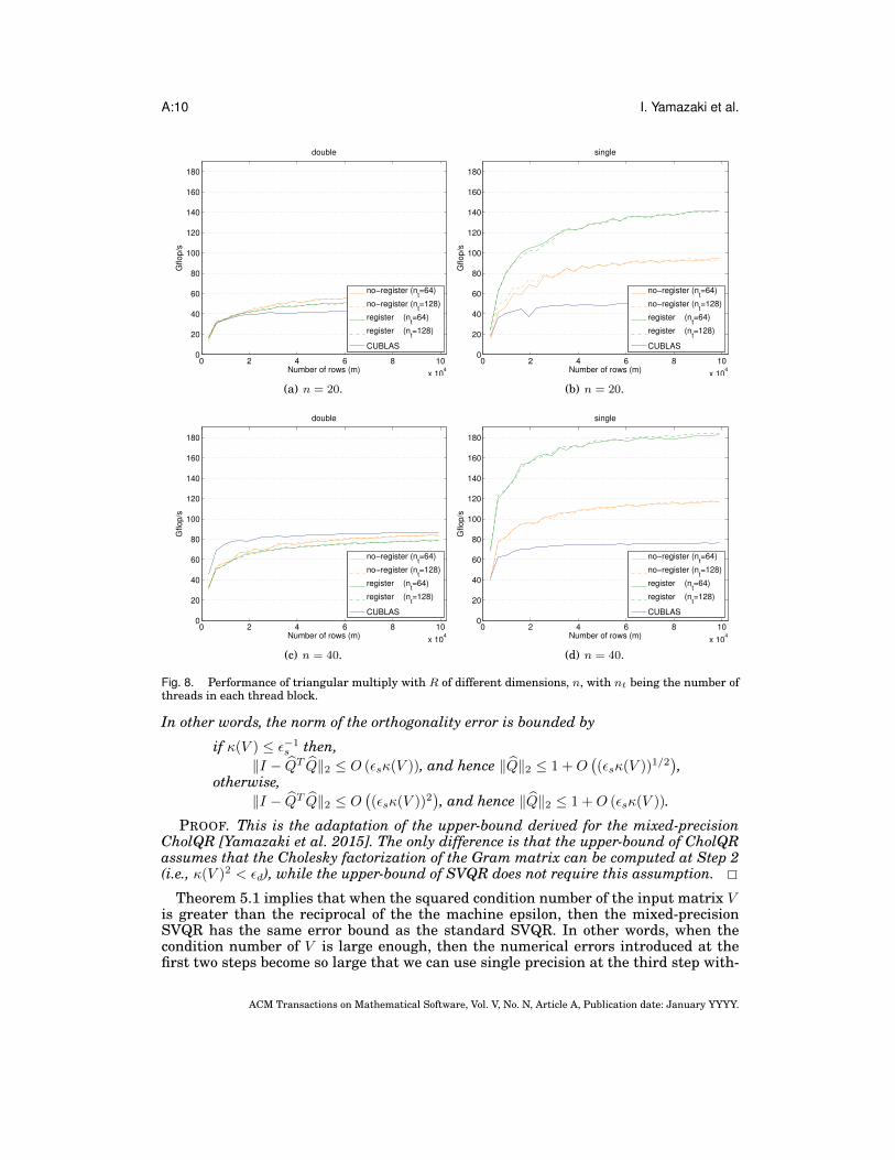
Fig. 8. Performance of triangular multiply with R of different dimensions, n, with nt being the number ofthreads in each thread block.

In other words, the norm of the orthogonality error is bounded by

if κ(V ) ≤ ε−1s then,‖I − Q̂T Q̂‖2 ≤ O (εsκ(V )), and hence ‖Q̂‖2 ≤ 1 +O

((εsκ(V ))1/2

),

otherwise,‖I − Q̂T Q̂‖2 ≤ O

((εsκ(V ))2

), and hence ‖Q̂‖2 ≤ 1 +O (εsκ(V )).

PROOF. This is the adaptation of the upper-bound derived for the mixed-precisionCholQR [Yamazaki et al. 2015]. The only difference is that the upper-bound of CholQRassumes that the Cholesky factorization of the Gram matrix can be computed at Step 2(i.e., κ(V )2 < εd), while the upper-bound of SVQR does not require this assumption.

Theorem 5.1 implies that when the squared condition number of the input matrix Vis greater than the reciprocal of the the machine epsilon, then the mixed-precisionSVQR has the same error bound as the standard SVQR. In other words, when thecondition number of V is large enough, then the numerical errors introduced at thefirst two steps become so large that we can use single precision at the third step with-



shared FloatingPoint t rA[N*N];int id = threadIdx.x;int ind = blockIdx.x * NB + threadIdx.x;

if (id < N) {#pragma unrollfor (int j=0; j<N; j++) rA(id,j) = dA(id,j);}

syncthreads();

if (ind < m) {FloatingPoint t rB[N];#pragma unrollfor (int j=0; j<N; j++) rB(j) = dB(ind,j);

#pragma unrollfor (int j=N-1; j>=0; j–) {

FloatingPoint t bij = ZERO;

for (int i=0; i<j; i++) bij += rA(i,j) * rB(i);rB(j) = bij + rA(j,j) * rB(j);}

#pragma unrollfor (int j=0; j<N; j++) dB(ind,j) = rB(j);}

(a) Pseudocode using registers to store B.

(b) TRSM’s access to R.

(c) TRMM’s access toR.

Fig. 9. Data access pattern and GPU implementation of triangular matrix multiply.

Step 1: Form Gram matrix BB := V TV in working precision

Step 2: Compute upper-triangular matrix R[U,Σ, U ] = svd(B) and[W,R] := qr(

√ΣUT ) in working precision

Step 3: Compute orthonormal matrix Qif σ1/σn ≥ 1/εd then

Q := V (d)R−1 in mixed-precisionelse

Q := V (d)R−1 in working precisionend if

(a) Pseudocode.

‖I −QTQ‖ ‖V −QR‖d-SVQR O(εdκ(V )2) O(εdκ(V ))

ds-SVQR O(εdκ(V )2 + εsκ(V )) O(εsκ(V ))(b) Error bounds.

Fig. 10. Pseudocode and error bounds of the mixed-precision SVQR.

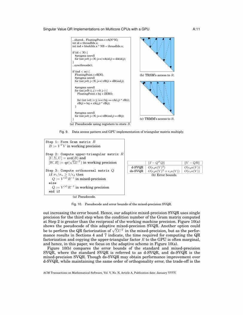
out increasing the error bound. Hence, our adaptive mixed-precision SVQR uses singleprecision for the third step when the condition number of the Gram matrix computedat Step 2 is greater than the reciprocal of the working machine precision. Figure 10(a)shows the pseudocode of this adaptive mixed-precision SVQR. Another option couldbe to perform the QR factorization of

√ΣUT in the mixed-precision, but as the perfor-

mance results in Sections 4 and 7 indicate, the time required for computing the QRfactorization and copying the upper-triangular factor R to the GPU is often marginal,and hence, in this paper, we focus on the adaptive scheme in Figure 10(a).

Figure 10(b) compares the error bounds of the standard and mixed-precisionSVQR, where the standard SVQR is referred to as d-SVQR, and ds-SVQR is themixed-precision SVQR. Though ds-SVQR may obtain performance improvement overd-SVQR, while maintaining the same order of orthogonality error, the trade-off is the



Name m n V κ(V )

K30(A,1) of 2D Laplacian A 1089 30 [1m, A1m, A21m, . . . , A301m] 3.5× 1019

Hilbert matrix 100 100 vi,j = (i+ j − 1)−1 6.6× 1019

Synthetic matrix 101 100 [1Tn ; diag(rand(n, 1) ∗ ε3d] 7.8× 1018

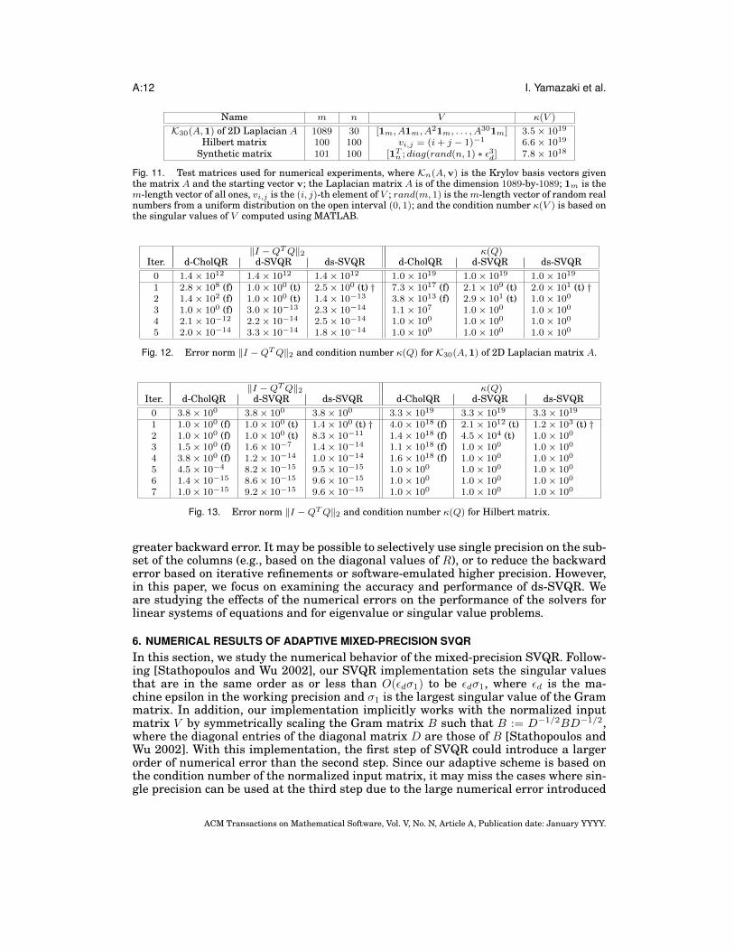
Fig. 11. Test matrices used for numerical experiments, where Kn(A,v) is the Krylov basis vectors giventhe matrix A and the starting vector v; the Laplacian matrix A is of the dimension 1089-by-1089; 1m is them-length vector of all ones, vi,j is the (i, j)-th element of V ; rand(m, 1) is them-length vector of random realnumbers from a uniform distribution on the open interval (0, 1); and the condition number κ(V ) is based onthe singular values of V computed using MATLAB.

‖I −QTQ‖2 κ(Q)Iter. d-CholQR d-SVQR ds-SVQR d-CholQR d-SVQR ds-SVQR0 1.4× 1012 1.4× 1012 1.4× 1012 1.0× 1019 1.0× 1019 1.0× 1019

1 2.8× 108 (f) 1.0× 100 (t) 2.5× 100 (t) † 7.3× 1017 (f) 2.1× 109 (t) 2.0× 101 (t) †2 1.4× 102 (f) 1.0× 100 (t) 1.4× 10−13 3.8× 1013 (f) 2.9× 101 (t) 1.0× 100

3 1.0× 100 (f) 3.0× 10−13 2.3× 10−14 1.1× 107 1.0× 100 1.0× 100

4 2.1× 10−12 2.2× 10−14 2.5× 10−14 1.0× 100 1.0× 100 1.0× 100

5 2.0× 10−14 3.3× 10−14 1.8× 10−14 1.0× 100 1.0× 100 1.0× 100

Fig. 12. Error norm ‖I −QTQ‖2 and condition number κ(Q) for K30(A,1) of 2D Laplacian matrix A.


1 1.0× 100 (f) 1.0× 100 (t) 1.4× 100 (t) † 4.0× 1018 (f) 2.1× 1012 (t) 1.2× 103 (t) †2 1.0× 100 (f) 1.0× 100 (t) 8.3× 10−11 1.4× 1018 (f) 4.5× 104 (t) 1.0× 100

3 1.5× 100 (f) 1.6× 10−7 1.4× 10−14 1.1× 1018 (f) 1.0× 100 1.0× 100

4 3.8× 100 (f) 1.2× 10−14 1.0× 10−14 1.6× 1018 (f) 1.0× 100 1.0× 100

5 4.5× 10−4 8.2× 10−15 9.5× 10−15 1.0× 100 1.0× 100 1.0× 100

6 1.4× 10−15 8.6× 10−15 9.6× 10−15 1.0× 100 1.0× 100 1.0× 100

7 1.0× 10−15 9.2× 10−15 9.6× 10−15 1.0× 100 1.0× 100 1.0× 100

Fig. 13. Error norm ‖I −QTQ‖2 and condition number κ(Q) for Hilbert matrix.

greater backward error. It may be possible to selectively use single precision on the sub-set of the columns (e.g., based on the diagonal values of R), or to reduce the backwarderror based on iterative refinements or software-emulated higher precision. However,in this paper, we focus on examining the accuracy and performance of ds-SVQR. Weare studying the effects of the numerical errors on the performance of the solvers forlinear systems of equations and for eigenvalue or singular value problems.

6. NUMERICAL RESULTS OF ADAPTIVE MIXED-PRECISION SVQRIn this section, we study the numerical behavior of the mixed-precision SVQR. Follow-ing [Stathopoulos and Wu 2002], our SVQR implementation sets the singular valuesthat are in the same order as or less than O(εdσ1) to be εdσ1, where εd is the ma-chine epsilon in the working precision and σ1 is the largest singular value of the Grammatrix. In addition, our implementation implicitly works with the normalized inputmatrix V by symmetrically scaling the Gram matrix B such that B := D−1/2BD−1/2,where the diagonal entries of the diagonal matrix D are those of B [Stathopoulos andWu 2002]. With this implementation, the first step of SVQR could introduce a largerorder of numerical error than the second step. Since our adaptive scheme is based onthe condition number of the normalized input matrix, it may miss the cases where sin-gle precision can be used at the third step due to the large numerical error introduced




1 1.0× 100 (f) 1.0× 100 (t) 1.0× 100 (t) † 2.9× 1017 (f) 4.4× 1010 (t) 4.4× 1010 (t) †2 6.5× 10−15 2.8× 10−8 1.0× 10−13 1.0× 100 1.0× 100 1.0× 100

3 5.4× 10−16 1.6× 10−14 1.1× 10−14 1.0× 100 1.0× 100 1.0× 100

4 4.4× 10−16 9.8× 10−15 8.9× 10−15 1.0× 100 1.0× 100 1.0× 100

5 4.4× 10−16 9.3× 10−15 8.4× 10−15 1.0× 100 1.0× 100 1.0× 100

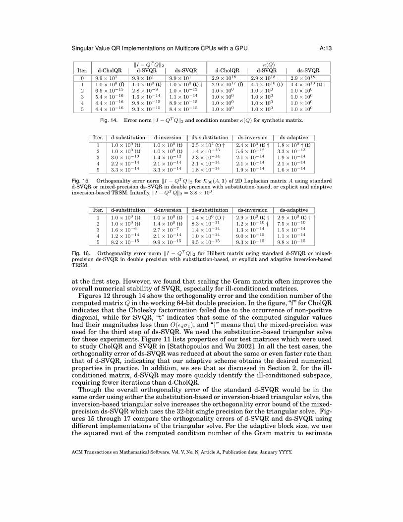
Fig. 14. Error norm ‖I −QTQ‖2 and condition number κ(Q) for synthetic matrix.

Iter. d-substitution d-inversion ds-substitution ds-inversion ds-adaptive1 1.0× 100 (t) 1.0× 100 (t) 2.5× 102 (t) † 2.4× 100 (t) † 1.8× 100 † (t)2 1.0× 100 (t) 1.0× 100 (t) 1.4× 10−13 5.6× 10−12 3.3× 10−13

3 3.0× 10−13 1.4× 10−12 2.3× 10−14 2.1× 10−14 1.9× 10−14

4 2.2× 10−14 2.1× 10−14 2.1× 10−14 2.1× 10−14 2.1× 10−14

5 3.3× 10−14 3.3× 10−14 1.8× 10−14 1.9× 10−14 1.6× 10−14

Fig. 15. Orthogonality error norm ‖I − QTQ‖2 for K30(A,1) of 2D Laplacian matrix A using standardd-SVQR or mixed-precision ds-SVQR in double precision with substitution-based, or explicit and adaptiveinversion-based TRSM. Initially, ‖I −QTQ‖2 = 3.8× 100.

Iter. d-substitution d-inversion ds-substitution ds-inversion ds-adaptive1 1.0× 100 (t) 1.0× 100 (t) 1.4× 100 (t) † 2.9× 100 (t) † 2.9× 100 (t) †2 1.0× 100 (t) 1.4× 100 (t) 8.3× 10−11 1.2× 10−10 † 7.5× 10−10

3 1.6× 10−6 2.7× 10−7 1.4× 10−14 1.3× 10−14 1.5× 10−14

4 1.2× 10−14 2.1× 10−14 1.0× 10−14 9.0× 10−15 1.1× 10−14

5 8.2× 10−15 9.9× 10−15 9.5× 10−15 9.3× 10−15 9.8× 10−15

Fig. 16. Orthogonality error norm ‖I − QTQ‖2 for Hilbert matrix using standard d-SVQR or mixed-precision ds-SVQR in double precision with substitution-based, or explicit and adaptive inversion-basedTRSM.

at the first step. However, we found that scaling the Gram matrix often improves theoverall numerical stability of SVQR, especially for ill-conditioned matrices.

Figures 12 through 14 show the orthogonality error and the condition number of thecomputed matrixQ in the working 64-bit double precision. In the figure, “f” for CholQRindicates that the Cholesky factorization failed due to the occurrence of non-positivediagonal, while for SVQR, “t” indicates that some of the computed singular valueshad their magnitudes less than O(εdσ1), and “†” means that the mixed-precision wasused for the third step of ds-SVQR. We used the substitution-based triangular solvefor these experiments. Figure 11 lists properties of our test matrices which were usedto study CholQR and SVQR in [Stathopoulos and Wu 2002]. In all the test cases, theorthogonality error of ds-SVQR was reduced at about the same or even faster rate thanthat of d-SVQR, indicating that our adaptive scheme obtains the desired numericalproperties in practice. In addition, we see that as discussed in Section 2, for the ill-conditioned matrix, d-SVQR may more quickly identify the ill-conditioned subspace,requiring fewer iterations than d-CholQR.

Though the overall orthogonality error of the standard d-SVQR would be in thesame order using either the substitution-based or inversion-based triangular solve, theinversion-based triangular solve increases the orthogonality error bound of the mixed-precision ds-SVQR which uses the 32-bit single precision for the triangular solve. Fig-ures 15 through 17 compare the orthogonality errors of d-SVQR and ds-SVQR usingdifferent implementations of the triangular solve. For the adaptive block size, we usethe squared root of the computed condition number of the Gram matrix to estimate



Iter. d-substitution d-inversion ds-substitution ds-inversion ds-adaptive1 1.0× 100 (t) 1.0× 100 (t) 1.0× 100 (t) † 6.3× 102 (t) † 1.0× 100 (t) †2 2.8× 10−8 2.8× 10−8 1.0× 10−13 4.2× 101 (t) † 1.5× 10−13

3 1.6× 10−14 1.5× 10−14 1.8× 10−6 1.8× 10−6 9.0× 10−15

4 9.8× 10−15 9.5× 10−15 8.9× 10−15 2.3× 10−14 9.2× 10−15

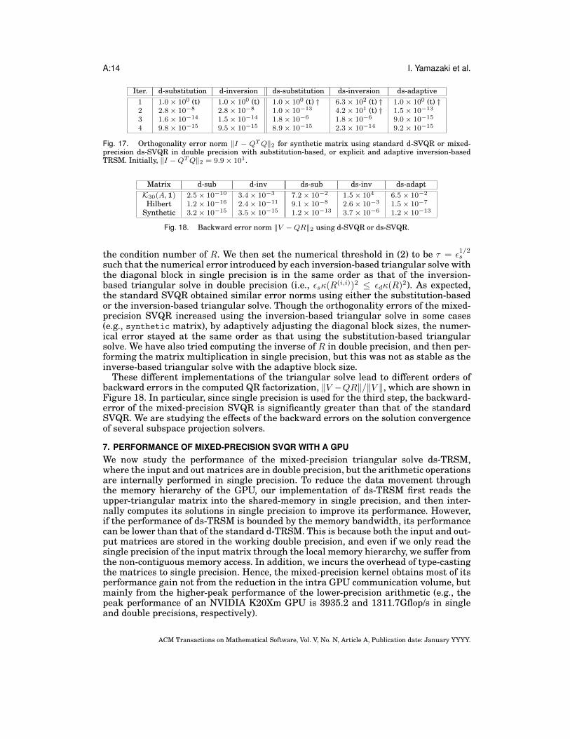
Fig. 17. Orthogonality error norm ‖I − QTQ‖2 for synthetic matrix using standard d-SVQR or mixed-precision ds-SVQR in double precision with substitution-based, or explicit and adaptive inversion-basedTRSM. Initially, ‖I −QTQ‖2 = 9.9× 101.

Matrix d-sub d-inv ds-sub ds-inv ds-adaptK30(A,1) 2.5× 10−10 3.4× 10−3 7.2× 10−2 1.5× 104 6.5× 10−2

Hilbert 1.2× 10−16 2.4× 10−11 9.1× 10−8 2.6× 10−3 1.5× 10−7

Synthetic 3.2× 10−15 3.5× 10−15 1.2× 10−13 3.7× 10−6 1.2× 10−13

Fig. 18. Backward error norm ‖V −QR‖2 using d-SVQR or ds-SVQR.

the condition number of R. We then set the numerical threshold in (2) to be τ = ε1/2s

such that the numerical error introduced by each inversion-based triangular solve withthe diagonal block in single precision is in the same order as that of the inversion-based triangular solve in double precision (i.e., εsκ(R(i,i))2 ≤ εdκ(R)2). As expected,the standard SVQR obtained similar error norms using either the substitution-basedor the inversion-based triangular solve. Though the orthogonality errors of the mixed-precision SVQR increased using the inversion-based triangular solve in some cases(e.g., synthetic matrix), by adaptively adjusting the diagonal block sizes, the numer-ical error stayed at the same order as that using the substitution-based triangularsolve. We have also tried computing the inverse of R in double precision, and then per-forming the matrix multiplication in single precision, but this was not as stable as theinverse-based triangular solve with the adaptive block size.

These different implementations of the triangular solve lead to different orders ofbackward errors in the computed QR factorization, ‖V −QR‖/‖V ‖, which are shown inFigure 18. In particular, since single precision is used for the third step, the backward-error of the mixed-precision SVQR is significantly greater than that of the standardSVQR. We are studying the effects of the backward errors on the solution convergenceof several subspace projection solvers.

7. PERFORMANCE OF MIXED-PRECISION SVQR WITH A GPUWe now study the performance of the mixed-precision triangular solve ds-TRSM,where the input and out matrices are in double precision, but the arithmetic operationsare internally performed in single precision. To reduce the data movement throughthe memory hierarchy of the GPU, our implementation of ds-TRSM first reads theupper-triangular matrix into the shared-memory in single precision, and then inter-nally computes its solutions in single precision to improve its performance. However,if the performance of ds-TRSM is bounded by the memory bandwidth, its performancecan be lower than that of the standard d-TRSM. This is because both the input and out-put matrices are stored in the working double precision, and even if we only read thesingle precision of the input matrix through the local memory hierarchy, we suffer fromthe non-contiguous memory access. In addition, we incurs the overhead of type-castingthe matrices to single precision. Hence, the mixed-precision kernel obtains most of itsperformance gain not from the reduction in the intra GPU communication volume, butmainly from the higher-peak performance of the lower-precision arithmetic (e.g., thepeak performance of an NVIDIA K20Xm GPU is 3935.2 and 1311.7Gflop/s in singleand double precisions, respectively).



0 2 4 6 8 10

x 104

0

20

40

60

80

100

120

Number of rows (m)

Gflop/s

s−TRSM

ds−TRSM (R in float)

ds−TRSM (R in double)

d−TRSM

(a) without cast/copy of R.

0 2 4 6 8 10

x 104

0

20

40

60

80

100

120

Number of rows (m)

Gflop/s

s−TRSM

ds−TRSM (R in float)


d−TRSM

(b) with cast/copy of R.

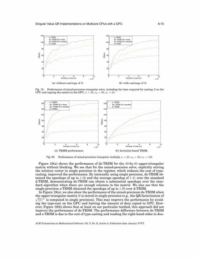
Fig. 19. Performance of mixed-precision triangular solve, including the time required for casting R on theCPU and copying the matrix to the GPU, n = 20, nb = 20, nt = 64.

0 2 4 6 8 10

x 104

0

20

40

60

80

100

120

140

Number of rows (m)

Gflop/s

s−TRMM

ds−TRMM (R in float)

ds−TRMM (R in double)

d−TRMM

(a) TRMM performance.

0 2 4 6 8 10

x 104

0

20

40

60

80

100

120

140

Number of rows (m)

Gflop/s

s−TRSM


d−TRSM

(b) Inversion-based TRSM.

Fig. 20. Performance of mixed-precision triangular multiply, n = 20, nb = 20, nt = 128.

Figure 19(a) shows the performance of ds-TRSM for the 20-by-20 upper-triangularmatrix without blocking. We see that for the mixed-precision solve, explicitly storingthe solution vector in single precision in the register, which reduces the cost of type-casting, improved the performance. By internally using single precision, ds-TRSM ob-tained the speedups of up to 1.56 and the average speedup of 1.41 over the standardd-TRSM, demonstrating ds-TRSM can obtain a substantial speedups over the stan-dard algorithm when there are enough columns in the matrix. We also see that thesingle-precision s-TRSM obtained the speedups of up to 1.99 over d-TRSM.

In Figure 19(a), we also show the performance of the mixed-precision ds-TRSM whenthe upper-triangular matrix R is stored in single precision (e.g., the QR factorization of√

ΣUT is computed in single precision). This may improve the performance by avoid-ing the type-cast on the GPU and halving the amount of data copied to GPU. How-ever, Figure 19(b) shows that at least on our particular testbed, this approach did notimprove the performance of ds-TRSM. The performance difference between ds-TRSMand s-TRSM is due to the cost of type-casting and reading the right-hand-sides in dou-



32000 160000 320000 480000 640000 8000000

0.1

0.2

0.3

0.4

0.5

0.6

0.7

0.8

0.9

1

Number of rows (m)

No

rma

lize

d T

ime

Step 3

Step 2

Step 1

(a) d-SVQR.

32000 160000 320000 480000 640000 8000000

0.1

0.2

0.3

0.4

0.5

0.6

0.7

0.8

0.9

1

Number of rows (m)

No

rma

lize

d T

ime

Step 3

Step 2

Step 1

(b) ds-SVQR.

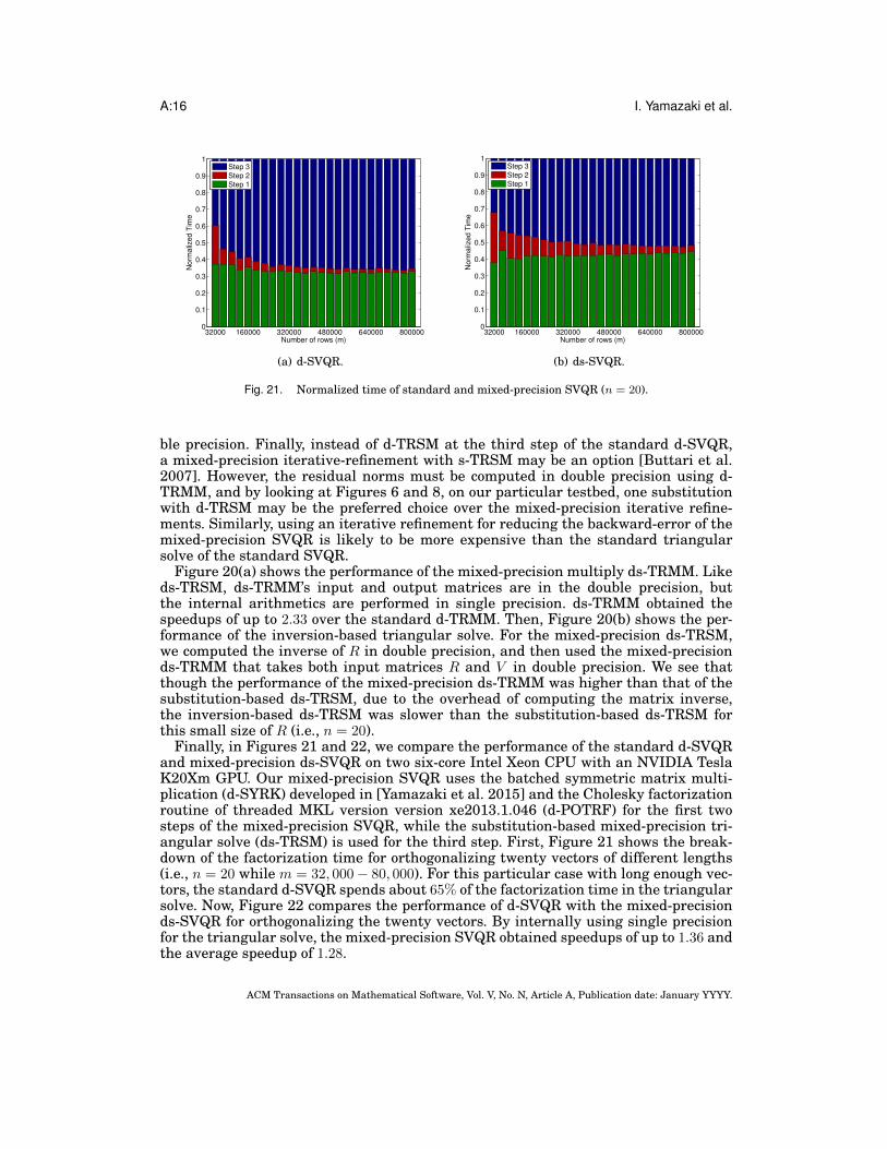
Fig. 21. Normalized time of standard and mixed-precision SVQR (n = 20).

ble precision. Finally, instead of d-TRSM at the third step of the standard d-SVQR,a mixed-precision iterative-refinement with s-TRSM may be an option [Buttari et al.2007]. However, the residual norms must be computed in double precision using d-TRMM, and by looking at Figures 6 and 8, on our particular testbed, one substitutionwith d-TRSM may be the preferred choice over the mixed-precision iterative refine-ments. Similarly, using an iterative refinement for reducing the backward-error of themixed-precision SVQR is likely to be more expensive than the standard triangularsolve of the standard SVQR.

Figure 20(a) shows the performance of the mixed-precision multiply ds-TRMM. Likeds-TRSM, ds-TRMM’s input and output matrices are in the double precision, butthe internal arithmetics are performed in single precision. ds-TRMM obtained thespeedups of up to 2.33 over the standard d-TRMM. Then, Figure 20(b) shows the per-formance of the inversion-based triangular solve. For the mixed-precision ds-TRSM,we computed the inverse of R in double precision, and then used the mixed-precisionds-TRMM that takes both input matrices R and V in double precision. We see thatthough the performance of the mixed-precision ds-TRMM was higher than that of thesubstitution-based ds-TRSM, due to the overhead of computing the matrix inverse,the inversion-based ds-TRSM was slower than the substitution-based ds-TRSM forthis small size of R (i.e., n = 20).

Finally, in Figures 21 and 22, we compare the performance of the standard d-SVQRand mixed-precision ds-SVQR on two six-core Intel Xeon CPU with an NVIDIA TeslaK20Xm GPU. Our mixed-precision SVQR uses the batched symmetric matrix multi-plication (d-SYRK) developed in [Yamazaki et al. 2015] and the Cholesky factorizationroutine of threaded MKL version version xe2013.1.046 (d-POTRF) for the first twosteps of the mixed-precision SVQR, while the substitution-based mixed-precision tri-angular solve (ds-TRSM) is used for the third step. First, Figure 21 shows the break-down of the factorization time for orthogonalizing twenty vectors of different lengths(i.e., n = 20 while m = 32, 000− 80, 000). For this particular case with long enough vec-tors, the standard d-SVQR spends about 65% of the factorization time in the triangularsolve. Now, Figure 22 compares the performance of d-SVQR with the mixed-precisionds-SVQR for orthogonalizing the twenty vectors. By internally using single precisionfor the triangular solve, the mixed-precision SVQR obtained speedups of up to 1.36 andthe average speedup of 1.28.



32000 160000 320000 480000 640000 8000000

1

2

3

4

5

6

7

8

9

Number of rows (m)

Tim

e (

ms)

Step 3

Step 2

Step 1

(a) d-SVQR.

32000 160000 320000 480000 640000 8000000

1

2

3

4

5

6

7

8

9

Number of rows (m)

Tim

e (

ms)

Step 3

Step 2

Step 1

(b) ds-SVQR.

Fig. 22. Performance of standard and mixed-precision SVQR (n = 20).

8. CONCLUSIONTo orthogonalize a set of dense column vectors, we studied the numerical stability andperformance of different Singular Value QR (SVQR) implementations. We focused onthe triangular solver which performs about half of the total floating-point operations ofthe orthogonalization process. Though we have integrated several optimization tech-niques into our GPU kernels, to reduce their communication overheads and increasethe benefit of using the mixed-precision kernels, we are looking to further tune theirperformance (e.g., using BEAST4). All the BLAS kernels developed for this study willbe released through the MAGMA library5. We are also working on the implementationof a communication-avoiding variant of Householder QR factorization (CAQR) [Dem-mel et al. 2012] on a GPU. Our implementation is based on a batched QR and GEMM,while our CholQR implementation was based on a batched SYRK and TRSM. Thoughperforming twice more flops, we are investigating how closely CAQR would performcompared to CholQR on a GPU, especially for tall-skinny matrix when the performancecan be limited by the memory bandwidth of the GPU.

As a part of the studies, we examined a mixed-precision variant that uses the halved-precision for the triangular solve. Our performance results on multicore CPUs with aGPU illustrated that though the intra GPU communication volume may not be re-duced, the mixed-precision variant can improve the performance by taking advantageof the higher peak-performance of the lower-precision arithmetic. Then, we describedan adaptive mixed-precision scheme to decide if the lower-precision can be used for thetriangular solve at run time. Compared to the standard SVQR, this adaptive mixed-precision SVQR maintains the same order of the orthogonality error, but significantlyincreases its backward error.6 We are currently studying the effects of the backwarderrors on various linear and eigenvalue solvers.

AcknowledgmentsThis research was supported in part by NSF SDCI - National Science FoundationAward #OCI-1032815, “Collaborative Research: SDCI HPC Improvement: Improve-

4http://icl.utk.edu/beast/5http://icl.utk.edu/magma/6We have studied several techniques to reduce the backward errors but on the current GPU architecture,the overhead of reducing the errors tends be greater than the performance improvement gained using thesingle precision.


http://icl.utk.edu/magma/


ment and Support of Community Based Dense Linear Algebra Software for Ex-treme Scale Computational Science,” DOE grant #DE-SC0010042: “Extreme-scale Al-gorithms & Solver Resilience (EASIR),” Russian Scientific Fund, Agreement N14-11-00190, and “Matrix Algebra for GPU and Multicore Architectures (MAGMA) for LargePetascale Systems.”

REFERENCESC. Bischof. 1990. Incremental condition estimation. SIAM J. Matrix Anal. Appl. 11 (1990), 312–322.A. Buttari, J. Dongarra, J. Langou, J. Langou, P. Luszczek, and J. Kurzak. 2007. Mixed Precision Iterative

Refinement Techniques for the Solution of Dense Linear Systems. Int. J. High Perform. Comput. Appl.21, 4 (2007), 457–466.

J. Demmel, L. Grigori, M. Hoemmen, and J. Langou. 2012. Communication-optimal parallel and sequentialQR and LU factorizations. SIAM J. Sci. Comput. 34, 1 (2012), A206–A239.

G. Golub and C. van Loan. 2012. Matrix Computations (4th ed.). The Johns Hopkins University Press,Baltimore, MD.

M. Hoemmen. 2010. Communication-avoiding Krylov subspace methods. Ph.D. Dissertation. EECS Depart-ment, University of California, Berkeley.

J. Kurzak, S. Tomov, and J. Dongarra. 2011. Autotuning GEMMs for Fermi. Technical Report UT-CS-11-671.Computer Science Department, University of Tennessee.

Y. Saad. 2003. Iterative methods for sparse linear systems (3 ed.). The Society for Industrial and AppliedMathematics, Philadelphia, PA.

Y. Saad. 2011. Numerical methods for large eigenvalue problems (2 ed.). The Society for Industrial andApplied Mathematics, Philadelphia, PA.

A. Stathopoulos and K. Wu. 2002. A block orthogonalization procedure with constant synchronization re-quirements. SIAM J. Sci. Comput. 23 (2002), 2165–2182.

J. van Rosendale. 1983. Minimizing inner product data dependence in conjugate gradient iteration. In Proc.IEEE Internat. Confer. Parallel Processing.

I. Yamazaki, H. Anzt, S. Tomov, M. Hoemmen, and J. Dongarra. 2014. Improving the performance of CA-GMRES on multicores with multiple GPUs. In the proceedings of the IEEE International Parallel andDistributed Symposium (IPDPS). 382–391.

I. Yamazaki, J. Kurzak, P. Luszczek, and J. Dongarra. 2015. Randomized algorithms to update partial sin-gular value decomposition on a hybrid CPU/GPU cluster. In Proceedings of the international conferencefor high performance computing, networking, storage and analysis (SC). 345–354.

I. Yamazaki, S. Rajamanickam, E. Boman, M. Hoemmen, M. Heroux, and S. Tomov. 2014. Domain decom-position preconditioners for communication-avoiding Krylov methods on a hybrid CPU/GPU cluster. Inthe proceedings of the international conference for high performance computing, networking, storage andanalysis (SC). 933–944.

I. Yamazaki, S. Tomov, and J. Dongarra. 2015. Mixed-precision Cholesky QR factorization and its case stud-ies on multicore CPUs with multiple GPUs. SIAM J. Scientific Computing (2015), C307–330.


A Stability and Performance of Various Singular Value QR ...

Documents

Transcript of A Stability and Performance of Various Singular Value QR ...