A SMALL DEFORMATION MODEL FOR THE ELASTO-PLASTIC … · 2006-09-20 · model for this...
81
Department of Mechanical Engineering Solid Mechanics ISRN LUTFD2/TFHF–06/5115–SE(1–81) A SMALL DEFORMATION MODEL FOR THE ELASTO-PLASTIC BEHAVIOUR OF PAPER AND PAPERBOARD Master’s Thesis by Tomas Andersson Supervisors Mikael Nyg˚ ards, STFI-Packforsk Anders Harrysson, Div. of Solid Mechanics Examiner Mathias Wallin, Div. of Solid Mechanics Copyright c 2006 by Div. of Solid Mechanics, STFI-Packforsk and Tomas Andersson. Printed by KFS i LUND AB, Lund, Sweden. For information, address: Division of Solid Mechanics, Lund University, Box 118, SE-221 00 Lund, Sweden. Homepage: http://www.solid.lth.se
Transcript of A SMALL DEFORMATION MODEL FOR THE ELASTO-PLASTIC … · 2006-09-20 · model for this...

Department of Mechanical Engineering
Solid Mechanics
ISRN LUTFD2/TFHF–06/5115–SE(1–81)
A SMALL DEFORMATION MODEL FORTHE ELASTO-PLASTIC BEHAVIOUR
OF PAPER AND PAPERBOARD
Master’s Thesis by
Tomas Andersson
SupervisorsMikael Nygards, STFI-Packforsk
Anders Harrysson, Div. of Solid Mechanics
ExaminerMathias Wallin, Div. of Solid Mechanics
Copyright c© 2006 by Div. of Solid Mechanics,
STFI-Packforsk and Tomas Andersson.
Printed by KFS i LUND AB, Lund, Sweden.
For information, address:
Division of Solid Mechanics, Lund University, Box 118, SE-221 00 Lund, Sweden.
Homepage: http://www.solid.lth.se


Acknowledgements
The master’s thesis presented in this paper has been carried out in partial fulfilment of thedegree Master of Science in Mechanical Engineering at Lund Institute of Technology. Thework has been carried out at STFI-Packforsk in Stockholm, Sweden during the autumnof 2005, with supervision from the Division of Solid Mechanics at Lund Institute of Tech-nology. Being part of the frontline of the paper research and development has gained memuch knowledge and it has been a fun and interesting experience for me.
First of all I would like to express my gratitude to the initiator of the project, PhD MikaelNygards. As my supervisor at STFI-Packforsk he has put in much effort in order to help,inspire and support me throughout the project. I especially appreciate our discussionsabout paper mechanisms and model building, and for always being willing to read throughmy uncountable drafts. I would like to thank my supervisor at Lund Institute of Technol-ogy, PhD candidate Anders Harrysson, for his mindful explanations when answering myquestions and for always getting me on the right track when answering my endless e-mails.I would like to show my appreciation to my examiner, PhD Mathias Wallin, for his interestin my work and I would especially like to thank him for the help on how to calculate thematerial stiffness tensor. Finally I would like to show my gratitude to Prof. Niels SaabyeOttosen for steering me onto the material modelling track in the first place.
A beautiful snow-white day in Lund, January 2006.
Tomas Andersson
i


Abstract
In order to optimize paper products and predict paper converting processes solid mechanicsanalyses can be conducted. In order to make accurate analyses reliable material modelsare required. In 2002 Q.S. Xia proposed a large deformation model for paperboard. Themodel consist of a continuum model that describes the behaviour of layers of fibres andan interface model that describes the delamination between layers of fibres. This master’sthesis attempts to contribute to the further development of a reliable material model.
Three major aspects have been covered within this work. First, a small deformation con-tinuum model for paper is proposed. Second, the proposed model is implemented into thecommercial finite element program ABAQUS/Standard. Third, to illustrate the behaviourof the model, a simulation of creasing of paperboard is performed.
The continuum model consist of two parts which are solved separately; the in-plane modeland the out-of-plane model. The in-plane model accounts for the behaviour of the twodirections in the paper-plane and the shear between these two directions. The out-of-planemodel controls the behaviour in the through-thickness direction of the paper and the shearbetween this direction and the two in-plane directions. The in-plane model proposed is asmall deformation formulation of the model proposed by Xia (2002). In the original modelby Xia (2002) the out-of-plane model does only has an elastic behaviour. The importanceto have an elasto-plastic behaviour in these components has however been recognized and amodel for this elasto-plastic behaviour have been developed. The behaviour of the normalcomponent in the thickness direction is inspired by a model proposed by Stenberg (2003),treats the paper as a porous material and accounts for nonlinear elasticity that dependsboth on the elastic strain and the plastic strain. The out-of-plane shear behaviour proposedis a model with linear elasticity and isotropic hardening. Furthermore, the report containscomments and explanations to why the model proposed by Stenberg (2003) for the out-of-plane behaviour is not appropriate.
The implementation of the theoretical model requires a development of an integrationscheme and, since ABAQUS/Standard uses an implicit approach, a material stiffness matrixconsistent with the integration scheme. This has been done and the Newton-Raphsonmethods used have achieved quadratic convergence, which makes the model fast and easyto work with.
iii

The simulations of creasing is done with the proposed continuum model together with theinterface model proposed by Xia (2002). The simulations shows an improvement comparedto the original model proposed by Xia (2002), mainly during unloading.

Contents
Acknowledgements i
Abstract iii
1 Introduction 11.1 Background . . . . . . . . . . . . . . . . . . . . . . . . . . . . . . . . . . . 11.2 Purpose of the assignment . . . . . . . . . . . . . . . . . . . . . . . . . . . 21.3 Notation . . . . . . . . . . . . . . . . . . . . . . . . . . . . . . . . . . . . . 2
2 Literature and experimental study 52.1 A short introduction to paper and paperboard . . . . . . . . . . . . . . . . 52.2 Experimental background . . . . . . . . . . . . . . . . . . . . . . . . . . . 8
2.2.1 In-plane behaviour . . . . . . . . . . . . . . . . . . . . . . . . . . . 82.2.2 Out-of-plane behaviour . . . . . . . . . . . . . . . . . . . . . . . . . 9
2.3 Short review of the 3DM model presented by Xia (2002) . . . . . . . . . . 102.3.1 Theory of the continuum model . . . . . . . . . . . . . . . . . . . . 122.3.2 Theory of the interface model . . . . . . . . . . . . . . . . . . . . . 16
3 Theory of continuum model in a small deformation formalism 233.1 Elastic strain of ortotropic materials and division into in-plane model and
out-of-plane model. . . . . . . . . . . . . . . . . . . . . . . . . . . . . . . . 233.2 In-plane model . . . . . . . . . . . . . . . . . . . . . . . . . . . . . . . . . 26
3.2.1 Yield criterion . . . . . . . . . . . . . . . . . . . . . . . . . . . . . . 263.2.2 Flow rule . . . . . . . . . . . . . . . . . . . . . . . . . . . . . . . . 273.2.3 Hardening . . . . . . . . . . . . . . . . . . . . . . . . . . . . . . . . 30
3.3 Out-of-plane model . . . . . . . . . . . . . . . . . . . . . . . . . . . . . . . 303.3.1 ZD compression . . . . . . . . . . . . . . . . . . . . . . . . . . . . . 313.3.2 Out-of-plane shear . . . . . . . . . . . . . . . . . . . . . . . . . . . 34
4 Implementation 374.1 Solution of equilibrium equation . . . . . . . . . . . . . . . . . . . . . . . . 384.2 Integration of constitutive equations . . . . . . . . . . . . . . . . . . . . . . 404.3 Material tangent stiffness matrix . . . . . . . . . . . . . . . . . . . . . . . 43
v

vi Contents
4.4 ABAQUS/Standard . . . . . . . . . . . . . . . . . . . . . . . . . . . . . . . 44
5 Simulations and results 475.1 Set-up in the simulations . . . . . . . . . . . . . . . . . . . . . . . . . . . . 475.2 Results . . . . . . . . . . . . . . . . . . . . . . . . . . . . . . . . . . . . . . 50
6 Discussion and conclusions 576.1 Further work . . . . . . . . . . . . . . . . . . . . . . . . . . . . . . . . . . 58
A Comments to the model proposed by Stenberg (2003) 65A.1 ZD compression . . . . . . . . . . . . . . . . . . . . . . . . . . . . . . . . . 65A.2 Shear model . . . . . . . . . . . . . . . . . . . . . . . . . . . . . . . . . . . 66
B Calculations used in the implementation 69B.1 In-plane model . . . . . . . . . . . . . . . . . . . . . . . . . . . . . . . . . 69
B.1.1 Material tangent stiffness components . . . . . . . . . . . . . . . . . 71B.2 Out-of-plane normal model . . . . . . . . . . . . . . . . . . . . . . . . . . . 71
B.2.1 Material tangent stiffness components . . . . . . . . . . . . . . . . . 72B.3 Out-of-plane shear model . . . . . . . . . . . . . . . . . . . . . . . . . . . . 72
B.3.1 Material tangent stiffness components . . . . . . . . . . . . . . . . . 73

Chapter 1
Introduction
1.1 Background
Paper is a widely used material with many advantages; it is cheap to manufacture, it isfairly strong considering the low weight, it can be recycled and it does not contain largeamounts of hazardous substances. It is a advantage to decrease the amount of raw materialin the paper products both from an economic point of view and an environmental point ofview. Solid mechanics analyses has been used in various areas to optimize products, andthere exists many different material models for all kinds of material. This type of analysescan also be used in order to optimize paper and paperboard products, but in order todo this an accurate model for the material is needed. Solid mechanics analyses has onlyrecently been introduced for calculation on paper and paperboard. The main reason forthis is that paper and paperboard is a complex material to model; mainly because it haslarge differences in properties between the different directions and the fibres delaminatewhen the paperboard deforms. The four main reasons for creating a material model inorder to do simulations on paper and paperboard are:
• Accurate predict outcome of converting processes.
• Establish important material properties, to get an idea of how the material will actwhen improvements of paper properties are achieved.
• Gather knowledge from experiments, to get an easy handled description of the paper.
• Understand the mechanisms of paper deformation.
STFI-Packforsk, which is the Swedish Pulp, Paper, Printing and Packaging Research Insti-tute located in Stockholm, Sweden, has together with contributing paper industry recog-nized the need to develop a material model for paper and paperboard. Therefore they havefor many years been involved in a large project that has involved experimental, theoreticaland numerical studies. The model developed, called the 3DM-model, is based on a large
1

2 Chapter 1. Introduction
deformation formalism, and was published as PhD thesis by Q.S. Xia at MassachusettsInstitute of Technology in the USA in 2002. The 3DM model consists of a continuumin-plane model that controls the behaviour in a layer of fibres in the paperboard and aninterface model that controls the delaminations between the layers of fibres.
1.2 Purpose of the assignment
The objective of this master’s thesis is to develop and implement a three dimensional con-tinuum material model for layers of paper fibres based on small deformations. The modelshould together with an existing delamination model capture the behaviour of paperboard.The model should also be tested to verify the accuracy of the model. This is done by:
• Adapting the continuum model presented by Xia (2002) into a model based on smalldeformations.
• Improving the model presented by Xia (2002) by adding plastic behaviour in thethrough-thickness direction of the paper.
• Choosing an appropriate implementation strategy.
• Implementing the model into the finite element program ABAQUS/Standard.
• Testing the model by building up a creasing procedure in ABAQUS and do simula-tions on the paperboard.
1.3 Notation
Two types of notation are used in the report. Bold symbols refer to variables that consistof more than one component and are used in general discussions when specific componentsare of minor importance. When we need to be more specific and refer to each componentindex notation is used. Index notation is a convenient way of writing complex formulas ina compact form. Each index takes the values 1, 2 and 3 if nothing else is stated. If twoindices are repeated in a term summation are applied, i.e.
Aij ⇔
A11 A12 A13
A21 A22 A23
A31 A32 A33
, (1.1)
Aii =3∑
i=1
Aii = A11 + A22 + A33. (1.2)

1.3. Notation 3
To illustrate the difference between index notation, to write out each component and boldnotation see example below.
AijXj = Bi ⇔
A11 A12 A13
A21 A22 A23
A31 A32 A33
X1
X2
X3
=
B1
B2
B3
⇒ AX = B (1.3)
In the report the Euclidean norm is used, defined as
‖x‖ =√
x21 + ... + x2
n if x = (x1, ..., xn). (1.4)

4 Chapter 1. Introduction

Chapter 2
Literature and experimental study
2.1 A short introduction to paper and paperboard
The main constituents when manufacturing paper and paperboard are fibre, water andenergy. Fibres from wood are by far the most common but fibres from grass and otherplants - and in rare occasions fibres from outside the flora - can be used. In Sweden allpaper mills uses wood as raw material. Wood contains fibres that hold together withlignin. When manufacturing paper the fibres need to be separated from each other. Thetwo main methods to separate the fibres are the mechanical method and the chemicalmethod. In the mechanical method the fibres are torn apart by adding mechanical energywith for example a grinding wheel. In the chemical method the fibres are separated byadding chemicals which resolve the lignin. With the mechanical method, the wood is betterpreserved since less of the lignin is removed. This also has the effect that paper made fromfibres separated with the mechanical method is weaker and turn yellow faster than papermade from chemical pulp. The methods can be combined and heat and water can be addedin the fibre separation to achieve different advantages and different properties in the paper.This is a big research area and numerous books have been written on the subject cf. Fellersand Norman (1998).
During or after the fibre separation process the fibres are resolved in water and this fibresuspension is sprayed onto a fast moving web, called a wire. In a pressing segment anda drying segment the water is drained out of the suspension and the fibres stick togetherwith hydrogen bridges, hence no adhesives needs to be added.
The manufacturing process has the effect that most of the fibres are oriented in the di-rection of the machine and that almost no fibres are oriented in the thickness direction.This phenomenon leads to the anisotropy of paper. The paper is usually treated as anorthotropic material and the three different directions of the paper machine are used asprincipal directions of the paper. The directions are illustrated in figure 2.1. The paper
5

6 Chapter 2. Literature and experimental study
is highly anisotropic with the stiffness in the Machine Direction (MD) being 1-5 timeslarger than in the Cross Direction (CD), and around 100 times larger than in the thicknessdirection (ZD).
Figure 2.1: Principal directions in paper.
Paper materials exhibit many exciting features making them complex to model. Thisis due to their highly anisotropic behaviour, non-linear inelastic material response anddependency on the moisture content of the material. Furthermore, inelastic delaminationbetween fibres occur when the paperboard deforms plastically, which makes a continuumapproach not valid for the entire paperboard when modelling detailed inelastic behaviourwhere delamination occur.
Thicker paper materials is usually called paperboard, but there exists no distinct definitionseparating paper from paperboard. As a reference material in this work a multilayeredpaperboard has been used. The paperboard is composed of five layers; three layers madeby mechanical pulp in the middle of the paperboard, and one outer chemical layer on eachside of the core, see figure 2.2. The paperboard is approximately 0.45 millimetres thick.
When converting paperboard into products such as packages the paperboard needs to befolded. An illustration of this procedure can be seen in figure 2.3. To get a nice foldthe paperboard is first punched with a male die (cf. figure 2.3.b), creating a straight lineof damage in the paperboard. When a bending moment is applied to the paperboard (cf.figure 2.3.d) the fold will preferentially fold along this line creating a straight and symmetriccrease.

2.1. A short introduction to paper and paperboard 7
Figure 2.2: Picture of paperboard showing the different layers.
Figure 2.3: Schematic of creasing and subsequent folding of paperboard. From Carlssonet al. (1983).

8 Chapter 2. Literature and experimental study
2.2 Experimental background
In order to understand the elastic and inelastic mechanisms of paper and paperboard severalexperimental studies have been performed. To mention a few Stenberg (2002a) has studiedthe behaviour in the out-of-plane direction, deRuvo et al. (1980) has studied the in-planebiaxial failure surface and Dunn (2000) has studied the micro-mechanical behaviour in aScanning Electron Microscope.
2.2.1 In-plane behaviour
The in-plane tensile behaviour for paperboard is presented in figure 2.4. These stress-straincurves plotted for MD, CD and an orientation 45◦ from MD clearly shows the anisotropicbehaviour of paperboard. The curves depict that MD has a factor 2-3 higher elastic mod-ulus and initial yield than CD. Tensile loading-unloading-reloading tests (Persson, 1991)
Figure 2.4: In-plane stress-strain curves, σf indicating failure stress. Adopted from Xia(2002).
show that the elastic tensile modulus is nearly unaffected by plastic strain, consistent withthe traditional elasto-plasticity theory.
To determine the yield surface of paper data from multi-axial tests is required. However,tests for the initial yield surface and the evolvement with the plastic strain has not beenexamined. Several researchers have however obtained biaxial failure surfaces; deRuvo et al.

2.2. Experimental background 9
(a) The modified Arcan device for measuring theout-of-plane behaviour of paperboard. The testsample is glued between the two parts of the front.LVDT stands for Linear Variable DisplacementTransducers and measures the displacements be-tween the two parts of the front.
(b) Arcan device for compression tests.
Figure 2.5: The modified Arcan device. From Stenberg (2002b).
(1980), Fellers et al. (1981) and Gunderson (1983). Since the experimental data for theyield surface is unavailable it is usually assumed that the yield surface exhibits the samecharacteristic as the failure surface.
2.2.2 Out-of-plane behaviour
The out-of-plane stress-strain behaviour of paperboard has been studied using a modifiedArcan (Arcan et al., 1978) device designed by Stenberg et al. (2001a). Figure 2.5(a) showsthe schematic of the design and figure 2.5(b) shows the set up for compression. The samplesmeasured 40 mm×15 mm for both compression and tension. A representative ZD tensilestress-strain curve for the paperboard obtained by Stenberg et al. (2001a) is shown infigure 2.6(b) The figure shows the peakload and subsequent softening. The stress-strainbehaviour in ZD compression has been studied by Stenberg (2002b) and a typical curvefor this behaviour is shown in figure 2.6(a). The curve shows the nonlinear elastic responseand that the elastic response depends on the plastic deformation of the paperboard.
When paperboard is creased, in order to soften the structure, initial cracks develop thatcauses the paperboard to more easily delaminate in the subsequent folding. The micro-mechanical mechanisms in paperboard, including delamination, has been studied by Dunn(2000). Figure 2.7 shows the delamination of paperboard in ZD tension. The initial de-lamination of paperboard in a creasing procedure is shown in figure 2.8. Up until thedelamination of the paperboard starts it can be a reasonable assumption to consider the

10 Chapter 2. Literature and experimental study
(a) A typical stress-strain curve for paperboard incompression, under consecutive through-thicknessloadings and unloadings. Adopted from Stenberg(2002b).
(b) A typical stress-strain curve for the paper-board in ZD tension. Adopted from Stenberg et al.(2001a).
Figure 2.6: Stress-strain response of paperboard in ZD.
paper as a homogeneous material as long as the considered length scale is reasonably large.When the cracks initiate the homogeneous assumption is however not valid.
(a) (b) (c)
Figure 2.7: ZD tension test of paperboard. View of the MD plane. Pictures taken withScanning Electron Microscope (SEM) by Dunn (2000).
2.3 Short review of the 3DM model presented by Xia
(2002)
Through the years different approaches have been applied to describe the properties ofpaperboard. The models fall into mainly three different categories; network models, lam-

2.3. Short review of the 3DM model presented by Xia (2002) 11
(a) Beginning of crease. (b) Male die at the deepest position.
(c) End of crease. White arrows indicating initialdelamination.
(d) Subsequent folding.
Figure 2.8: Crease and subsequent fold of paperboard across MD. Pictures taken with SEMby Dunn (2000).

12 Chapter 2. Literature and experimental study
inate models and continuum models. The models have advantages and disadvantages butnone of them completely captures the behaviour of paperboard. The approach used by Xia(2002) is to use a continuum model together with an interface model. A schematic modelof paperboard as presented by Xia (2002) can be seen in figure 2.9. The continuum modelcan in a sense be seen as the constitutive model for the mat of fibres in a plane, while theinterface model accounts for the delamination between the mats of fibres.
Figure 2.9: Schematics of Paperboard.
2.3.1 Theory of the continuum model
The continuum model proposed by Xia (2002) is controlling the behaviour of the mat offibres. The model consist of the three components for the normal stress and strain in thethree directions; and the the three components for the shear between these directions. Inthe model presented by Xia (2002) the components for compression and tension in MD andCD and the shear between the two have an elasto-plastic behaviour. This is henceforthreferred to as the in-plane model. The compression and tension in ZD and the shearbetween ZD and the two in-plane directions has in the 3DM-model an elastic behaviour.The model for these three components is henceforth referred to as the out-of-plane model.
The elastic behaviour in the in-plane model is linear and orthotropic. The yield surfaceevolves with the plastic strain with an isotropic hardening, meaning that the yield surfacedoes only depend on the magnitude of the plastic strain and not on the direction. Theplastic flow is modelled with an associate flow rule1. The model is formulated in a large
1Strictly, the flow rule is not associate since the flow rule is not energy conjugate as reported byRistinmaa (2003)

2.3. Short review of the 3DM model presented by Xia (2002) 13
deformation formalism. In this section the theory of the model is outlined. For more detailsabout the theory and how the model should be calibrated cf. Ristinmaa (2003).
Stress-strain relationship
The displacement of a particle can be described by considering the particle’s referenceposition in a coordinate system, X, and its current position, x according to figure 2.10.The displacement, u, is then defined as
u = x−X. (2.1)
Two neighbouring particles at a reference configuration in a continuous body can be
Figure 2.10: Displacement ui from the reference configuration, Xi, to the current configu-ration, xi.
identified by their positions X and X + dX where X denotes a position vector and dXthe distance between the particles. After deformation of the body the new distance betweenthe particles is dx. It is possible to describe the change from the reference configurationto the current configuration without including the rigid body motion according to
dx =∂x
∂XdX = F dX, (2.2)
where F is the linear mapping known as the deformation gradient, cf. figure 2.11. To makethe mapping unique it is assumed that det(F ) > 0.
With equation (2.1) and equation (2.2) it is seen that the deformation gradient can alsobe written as
F =∂x
∂X=
∂
∂X(X + u) = I +
∂u
∂X. (2.3)

14 Chapter 2. Literature and experimental study
Figure 2.11: Deformation of a continuous body.
It is assumed that at each material point the total deformation gradient can be multi-plicatively decomposed into an elastic part, F e, and a plastic part, F p, (cf. figure 2.12)hence
F = F eF p. (2.4)
When large deformations are considered many different strain measures exist. The optimal
Figure 2.12: Schematic representation of the multiplicative decomposition into elastic andplastic parts.
choice of strain depends on the material behaviour and type of analysis and there is notrue strain as there is a true stress. The model uses the Green strain2, εG, defined as
εG ≡1
2(F TF − I) =
1
2
(∂ui
∂Xj
+∂uj
∂Xi
+∂uk
∂Xi
∂uk
∂Xj
). (2.5)
According to Xia (2002) the second Piola-Kirchoff stress in the intermediate configuration,T, is related to the elastic Green strain, εe
G using the linear relationship
T = CεeG, (2.6)
2This strain measure is computationally convenient for problems involving large motions but smallstrains, since it can be computed directly from the deformation gradient.(ABAQUS, 2004)
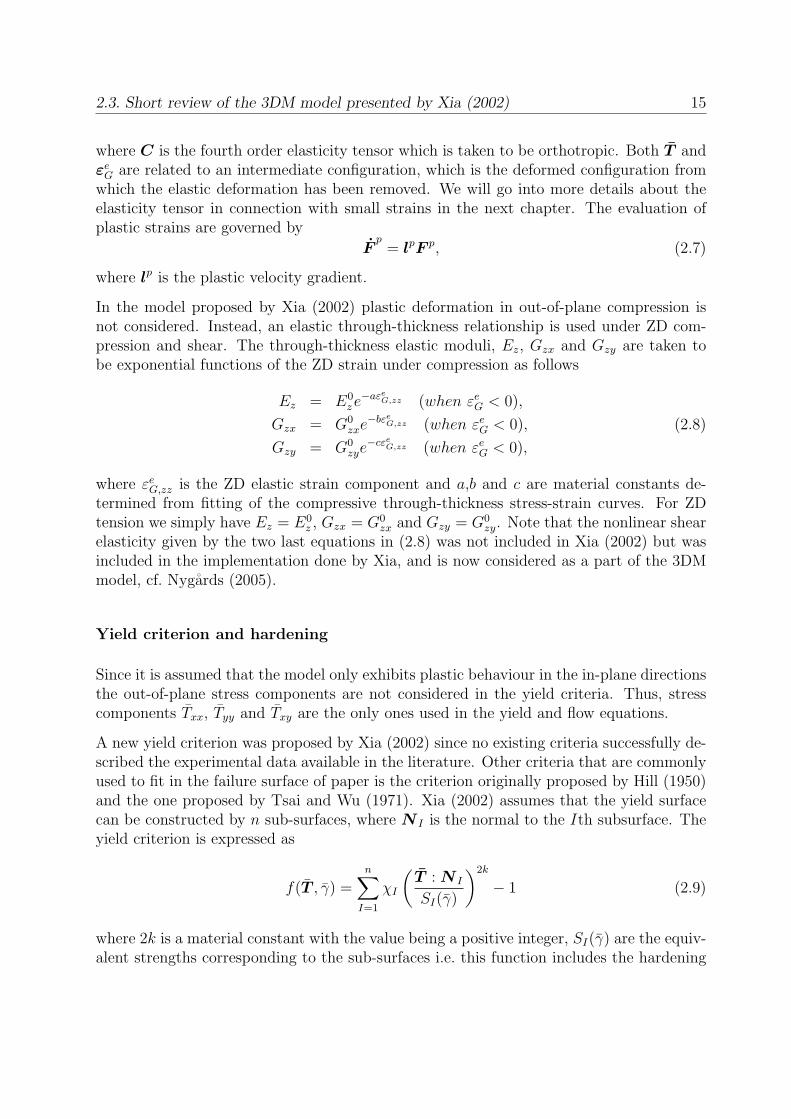
2.3. Short review of the 3DM model presented by Xia (2002) 15
where C is the fourth order elasticity tensor which is taken to be orthotropic. Both T andεe
G are related to an intermediate configuration, which is the deformed configuration fromwhich the elastic deformation has been removed. We will go into more details about theelasticity tensor in connection with small strains in the next chapter. The evaluation ofplastic strains are governed by
Fp
= lpF p, (2.7)
where lp is the plastic velocity gradient.
In the model proposed by Xia (2002) plastic deformation in out-of-plane compression isnot considered. Instead, an elastic through-thickness relationship is used under ZD com-pression and shear. The through-thickness elastic moduli, Ez, Gzx and Gzy are taken tobe exponential functions of the ZD strain under compression as follows
Ez = E0ze−aεe
G,zz (when εeG < 0),
Gzx = G0zxe
−bεeG,zz (when εe
G < 0), (2.8)
Gzy = G0zye
−cεeG,zz (when εe
G < 0),
where εeG,zz is the ZD elastic strain component and a,b and c are material constants de-
termined from fitting of the compressive through-thickness stress-strain curves. For ZDtension we simply have Ez = E0
z , Gzx = G0zx and Gzy = G0
zy. Note that the nonlinear shearelasticity given by the two last equations in (2.8) was not included in Xia (2002) but wasincluded in the implementation done by Xia, and is now considered as a part of the 3DMmodel, cf. Nygards (2005).
Yield criterion and hardening
Since it is assumed that the model only exhibits plastic behaviour in the in-plane directionsthe out-of-plane stress components are not considered in the yield criteria. Thus, stresscomponents Txx, Tyy and Txy are the only ones used in the yield and flow equations.
A new yield criterion was proposed by Xia (2002) since no existing criteria successfully de-scribed the experimental data available in the literature. Other criteria that are commonlyused to fit in the failure surface of paper is the criterion originally proposed by Hill (1950)and the one proposed by Tsai and Wu (1971). Xia (2002) assumes that the yield surfacecan be constructed by n sub-surfaces, where N I is the normal to the Ith subsurface. Theyield criterion is expressed as
f(T , γ) =n∑
I=1
χI
(T : N I
SI(γ)
)2k
− 1 (2.9)
where 2k is a material constant with the value being a positive integer, SI(γ) are the equiv-alent strengths corresponding to the sub-surfaces i.e. this function includes the hardening

16 Chapter 2. Literature and experimental study
of the model, γ is the equivalent plastic strain defined as γ =∫
˙γdt and χI is a switchingcontrol with the properties
χI =
{1 if T : N I > 0;0 otherwise.
(2.10)
Xia (2002) assumes that the yield strength evolution can be fitted to
SI(γ) = SI0 + A1tanh(B1γ) + C1γ, (2.11)
SII(γ) = SII0 + A2tanh(B2γ) + C2γ, (2.12)
SIII(γ) = SIII0 + A3tanh(B3γ) + C3γ, (2.13)
SIV (γ) = SIV0 + A4tanh(B4γ) + C4γ, (2.14)
SV (γ) = SV0 + A5tanh(B5γ) + C5γ, (2.15)
SV I(γ) = SIII(γ). (2.16)
In connection with small deformations in the next chapter the yield surface will be moreextensively described.
Evolution laws
The plastic flow is defined aslp = γK, (2.17)
where lp is the plastic velocity gradient. γ is the magnitude of plastic stretching rate, andK is the normalized flow direction and is calculated as
K =K
||K||, (2.18)
where K is the derivative of the yield surface and is assumed to be
K =∂f
∂T. (2.19)
With the aid of the yield surface, the yield direction can be calculated as
K =∂f
∂T= 2k
n∑I=1
(T : N I
SI(γ)
)2k−1
χIN I
SI(γ). (2.20)
2.3.2 Theory of the interface model
It is outside the scope of this report to go into details in the interface model. However,the model is used in the simulations of creasing and folding of paperboard. Therefore, asummary of the theoretical framework behind the model is presented.

2.3. Short review of the 3DM model presented by Xia (2002) 17
The model is important since two major mechanisms dominate during deformation ofpaperboard, namely elasto-plastic deformation within plies and delamination between plies.Just one continuum model can not capture the plastic behaviour in paperboard in shear.To illustrate this let us consider a two dimensional model of paper in the ZD-MD directionmodelled with a continuum model, cf. figure 2.13. In a model like this the three components
Figure 2.13: A continuum element subjected to shear.
of importance are ZD, MD and the shear between MD and ZD. In a continuum model theMD-ZD shear is not different from the ZD-MD shear3. We know that the plies slip easierin the direction of the fibres. Hence a unit of shear strain along the fibres, εZD,MD, causeslower shear stress along the fibre, σZD,MD, than a unit of shear strain across the fibres,εMD,ZD, causes the stress across the fibres, σMD,ZD. However, this is as mentioned earlierimpossible with only one continuum model.
The delamination model in this work has been proposed by Xia (2002). The model istraction-displacement based and models an elasto-plastic cohesive law between two oppos-ing surfaces. The model is used between the layers of in-plane elements (layers of fibresin real life paper4) and takes care of the delamination between the fibres. To simplify theunderstanding of the theory consider an interface between two plies in a paperboard asdepicted in Figure 2.14. At each point of the interface we introduce a local coordinatesystem where n is normal to the interface and t1 and t2 are orthogonal tangents to theinterface. The t1- and t2-directions usually corresponds to the MD and CD directions ofpaperboard, respectively. For brevity in the equation expressions, let 1, 2 and 3 denote n,t1 and t2.
3This is the reason why engineering shear strains can be used which are defined γxy = εxy +εyx = 2εxy.As curiosity it can be mentioned that in gradient theory polarities can occur that makes σxy 6= σyx
4Although in simulations an approximation is introduced, since the layers where the interface modelis introduced and the model is allowed to delaminate, is usually fewer than the delamination areas in thepaperboard.

18 Chapter 2. Literature and experimental study
Figure 2.14: An interface between two paperboard plies.
Indices indicated by Greek letters imply that no summation should be carried out overrepeated indices. Whenever other indices are used summation according to the summationconvention explained in section 1.3 should be used, i.e.
aαbα = aαbα (no summation), (2.21)
aibi =n∑
i=1
aibi. (2.22)
Kinematics
It is assumed that the displacement between two opposing surfaces can be divided into anelastic part and a plastic part. Thus, with reference to a local coordinate system at theinterface each displacement component can be expressed as
δi = δei + δp
i . (2.23)
Constitutive equations
According to Xia (2002) a change in traction across the interface due to an incrementalchange of displacements is expressed as
∆Tα = Kα (∆δα −∆δpα) , (2.24)

2.3. Short review of the 3DM model presented by Xia (2002) 19
where Kα denotes the components of the instantaneous interface stiffness in the α-direction.The instantaneous interface stiffness will decrease as the interface deforms. It depends onthe equivalent plastic displacement (δp) according to
Kα(δp) = K0α
(1− χRk
αD(δp)), (2.25)
where K0α is the initial interface stiffness and D(δp) is the interface damage. It is a positive
scalar that is derived as
D(δp) = tanh
(δp
δp0
)= tanh
(δp
C
). (2.26)
Hence, the model accounts for a reduced stiffness of the interface as damage evolves inthe interface. In equation (2.25) Rk
α and C are material constants, and the incrementalequivalent plastic displacement in Eq. (2.26) is expressed as
∆δp = ‖∆δpi ‖ . (2.27)
The interface is formulated to account for delamination in tension and shear. It is not atall desired to have overlapping of the surfaces when loaded in ZD compression. Therefore,penalty functions are used to prevent overlapping under such circumstances.
Yield criterion
Since the delamination model is elasto-plastic a yield condition is introduced. The yieldcondition is equivalent with a yield surface, but is expressed in terms of tractions. Theproposed yield conditions rely on experimental data by Stenberg (2002a), and Xia (2002)expressed that yielding occurs when
f(T, δp) =n∑
α=2
S1T2α
Sα(δp)2+ T1 − S1 = 0, (2.28)
where Sα(δp) are the instantaneous interface strengths that depend on the equivalent plasticdisplacement, δp, according to
Sα(δp) = S0α
(1− χRs
αD(δp)), (2.29)
where S0α are the initial interface strengths. In equation (2.28) n is used to distinguish
between the 2-D case and 3-D case. In the 2-D case n equals 2, while in the 3-D case n isequal to 3. In figure 2.15 the two dimensional yield surface is plotted.

20 Chapter 2. Literature and experimental study
Figure 2.15: The yield surface in the case T3=0.
Flow rule
According to Xia (2002) the plastic flow rule is written as
∆δpi = χ∆δpMi (2.30)
where Mi are the components of the unit flow direction, i.e.
Mi =Mi
||M ||(2.31)
and χ indicates if there is plastic deformation in the interface, it is defined as
χ =
{1 if f = 0 and dT ∗ · ∂f
∂T> 0;
0 if f < 0 or f = 0 and dT ∗ · ∂f∂T
< 0.(2.32)
For associated flow the components of the plastic flow direction is derived as
M1 =∂f
∂T1
= 1 (2.33)
Mα =∂f
∂Tα
= 2S1(δ
p)
Sα(δp)2Tα. α = 2, 3 (2.34)
The associated flow will cause some normal dilation under the action of only shear stress,because of the shape of the traction yield surface. However, it is experimentally observedthat the dilation in paperboard exceeds the dilation caused by associate flow. Therefore,a non-associate flow is used to capture the observed behaviour. For the non-associate flowthe normal component of the flow direction is instead defined as
M1 = µ(δp)∂f
∂T1
, (2.35)

2.3. Short review of the 3DM model presented by Xia (2002) 21
where µ is a frictional function, plotted in figure 2.16 defined as
µ(δp) = A(1−BD(δp)). (2.36)
A and B are constants. D(δp) is the parameter controlling the damage of the interfaceaccording to equation (2.26).5
Figure 2.16: The frictional function plotted with parameters from Xia (2002).
5With the parameters for the frictional function fitted by Xia (2002) the non-associate flow rule proposedactually has lower normal dilation than for an associate flow rule as can be seen in figure 2.16, whichcontradicts the written purpose.

22 Chapter 2. Literature and experimental study

Chapter 3
Theory of continuum model in asmall deformation formalism
In this chapter the theory of a continuum model based on small deformations is presented.In section 3.1 the Generalized Hooke’s law is presented and the elastic response for paperis outlined. In section 3.2 a model for the in-plane components will be proposed that isa small deformation version of the model proposed by Xia (2002). In section 3.3 a modelfor the out-of-plane components will be proposed where the paperboard is treated as afoam-like material when compressed in the thickness direction.
3.1 Elastic strain of ortotropic materials and division
into in-plane model and out-of-plane model.
We are interested in the response of paper and paperboard when loads and displacementsare applied to the structure. For this we need to relate the kinematics of the structure tothe stress in the structure. The strain is the link between the kinematics and the materialmodel. If we recall the definition of the Green strain,
εG ≡1
2
(∂ui
∂Xj
+∂uj
∂Xi
+∂uk
∂Xi
∂uk
∂Xj
), (3.1)
where no assumptions were made. The strain in small deformations, ε, relates the defor-mation of the body to the original configure and the assumptions of small strains cancelout the quadratic terms in equation (3.1) and we get
εij =1
2
(dui
dXj
+duj
dXi
). (3.2)
23

24 Chapter 3. Theory of continuum model in a small deformation formalism
Figure 3.1: Schematics of Paperboard.
The total strain can be divided in an elastic part and a plastic part.
εij = εeij + εp
ij (3.3)
The relation that couples strain to stress, the constitutive model, describes the material.In 1676 Robert Hooke proposed a linear constitutive equation for the one dimensional case,σ = Eεe. This equation in its most general form is known as the Generalized Hooke’s law,
σij = Dijklεekl. (3.4)
where σij is the stress tensor which is defined as force acting on area of the original con-figuration. Dijkl is the constant elastic stiffness tensor. Equation (3.4) and (3.3) gives
σij = Dijkl (εkl − εpkl) . (3.5)
In static solid mechanics this equation forms a stable ground on which to build. Thetensor Dijkl introduced in equation (3.4) has 81 components but with energy considerations,geometrical considerations and considerations of the first law of thermodynamics it can beshown that a material can have no more than 21 independent components. Currently thereis no useful engineering materials with 21 different and independent components (Lagace,2005). Linear elastic orthotropic materials have 9 independent components, and equation

3.1. Elastic strain of ortotropic materials and division into in-plane model andout-of-plane model. 25
(3.4) can be written asσxx
σyy
σzz
σxy
σxz
σyz
=
1−νyzνzy
EyEz∆
νyx+νzxνyz
EyEz∆
νzx+νyxνzy
EyEz∆0 0 0
νxy+νxzνzy
EzEx∆1−νzxνxz
EzEx∆
νzy+νzxνxy
EzEx∆0 0 0
νxz+νxyνyz
ExEy∆
νyz+νxzνyx
ExEy∆
1−νxyνyx
ExEy∆0 0 0
0 0 0 Gxy 0 00 0 0 0 Gxz 00 0 0 0 0 Gyz
εe
xx
εeyy
εezz
γexy
γexz
γeyz
(3.6)
with
∆ =1− νxyνyx − νyzνzy − νzxνxz − 2νxyνyzνzx
ExEyEz
. (3.7)
In equation (3.6) engineering shear strain is used and this will be used in the remainder ofthe report. Engineering shear strain is related to tensorial shear strain according to
ε =
εxx
εyy
εzz
2εxy
2εxz
2εyz
=
εxx
εyy
εzz
γxy
γxz
γyz
. (3.8)
From the definition of orthotropic materials equation (3.6) is symmetric. Hence the elasticPoisson’s ratios and the elastic moduli are related according to
νxy
Ex
=νyx
Ey
, (3.9)
νxz
Ex
=νzx
Ez
, (3.10)
νyz
Ey
=νzy
Ez
, (3.11)
where Ex, Ey and Ez are the Young’s moduli in the principal directions. The Poisson’sratios, νij, is defined as
νij = −εjj
εii
(no summations). (3.12)
The out-of-plane Poisson’s ratio in paper has been reported as both positive and negative(Ohrn, 1965; Baumgarten and Gottsching, 1973; Mann et al., 1980; Persson, 1991; Stenbergand Fellers, 2002), with the reports for most of the papers tested having a negative Poisson’sratio. The tests are however difficult to perform with many possible errors and whenmodelling paper the out-of-plane Poisson’s ratios are often considered zero (Stenberg, 2003;Nygards, 2005). Also in this model this assumption will be utilized, hence
νyx = νxy = νyz = νzy = 0. (3.13)

26 Chapter 3. Theory of continuum model in a small deformation formalism
Since the out-of-plane Poisson’s ratios are zero and the out-of-plane properties are assumednot to depend on the in-plane state and vice versa. The in-plane and out-of-plane problemcan be separated and solved independently. Thus, the in-plane problem is formulated as σxx
σyy
σxy
=
Ex
1−νxyνyx
νyxEx
1−νxyνyx0
νxyEy
1−νxyνyx
Ey
1−νxyνyx0
0 0 Gxy
εxx
εyy
γxy
. (3.14)
The out-of-plane problem takes the form σzz
σxz
σyz
=
Ez 0 00 Gxz 00 0 Gyz
εezz
γexz
γeyz
. (3.15)
It should be noted that the linear relation in the through-thickness direction implied byequation (3.15) does not hold, as can be seen in figure 2.6(a). Instead a nonlinear expressionis needed to capture the nonlinear out-of-plane elasticity of paperboard.
3.2 In-plane model
The in-plane model correlates the two in-plane normal strain components (εxx and εyy) andthe in-plane shear strain component (γxy) to the corresponding stress components (σxx, σyy
and σxy). The elastic response is governed by equation (3.14).
3.2.1 Yield criterion
The yield criterion tests if plasticity develops. The response is elastic inside the yieldsurface. In this work the yield criterion proposed by Xia (2002) is utilized, which in smalldeformations is formulated as
f(σ, εpeff ) =
n∑I=1
χI
(σ : NI
σIs(ε
peff )
)2k
− 1. (3.16)
This yield surface is constructed by n yield planes. Xia (2002) uses six yield planes, one forevery ”direction” (i.e. σxx tension, σxx compression, σyy tension, σyy compression, positiveτxy and negative τxy). Each yield plane is defined by the out pointing normal, N , andthe parameter controlling the size of the yield surface, σs. σs (σs0 at the initial state)is defined, for the four planes for compression and tension, as the perpendicular distancefrom the origin to the plane yield planes, cf. figure 3.2. According to Xia (2002) this isalso the definition for yield planes corresponding to shear, this is however not true. This
distance for the shear planes is just σIIIs
2NIII13
, or with the calibration procedure proposed by

3.2. In-plane model 27
Xia (2002) - and described in the next section - σIIIs√2
i.e. around 71% of σIIIs . In conclusion,
it is important to note that σs0 (S0 for large deformations) is not the yield stress in thedifferent directions as it is sometimes mistaken for in the literature. The exponent 2k isgoverning the smoothening between the planes, a higher k results in a sharper edge, cf.figure 3.2. In equation (3.16) χI is a switch controller,
Figure 3.2: Yield surface with different k-values with the remaining parameters set for themechanical ply proposed by Xia (2002), and σxy = 0.
χI =
{1 if σ : NI > 0;0 otherwise.
(3.17)
In the model, the size of the yield surface is controlled by one parameter, namely theeffective plastic strain εp
eff defined in the next section. Figure 3.3 shows how the yieldsurface evolves with the plastic strain, when the hardening parameters for the mechanicalply proposed by Xia (2002) is used.
3.2.2 Flow rule
Once the yield surface is reached the material starts to flow, and plasticity develops. Thedirection of the flow is in the model perpendicular to the yield surface
K =∂f
∂σ. (3.18)

28 Chapter 3. Theory of continuum model in a small deformation formalism
Figure 3.3: Yield surface at different εpeff with parameters for the mechanical ply proposed
by Xia (2002).
Hence the flow is associated. The flow is normalised to give a magnitude of one unit in theflow direction K,
K =K∥∥∥K∥∥∥ . (3.19)
The rate of the plastic flow1 isεp = λK, (3.20)
where λ is the plastic multiplier2. When determining the normal directions (N ) to the sub-surfaces in the yield criterion, use is made of the fact that we have associate flow and theassumption that only one yields surface is active3 for uniaxial tension, uniaxial compressionand pure shear. In this way the direction of plastic flow in uniaxial tests coincide with N .
To give a short idea how N is calculated we consider uniaxial MD tension and calculate
1It should be noted that the model is statical, no dynamical effects or time dependencies occur. Thedenominator dt in for example λ = dλ
dt can be cancelled out and give the incremental form dλ. Theincremental form shows a change in property rather than a change in time. This is a convenient andwidely used notation.
2The plastic multiplier can be compared with the Lagrange multiplier that shows up in more generalcases outside the solid mechanics.
3The assumption that only one sub-surface is active is not strictly true as can be seen in figure 3.2, butfor high values of k this is a reasonable assumption.

3.2. In-plane model 29
the normal direction to the corresponding sub-surface (N I). It is assumed that there isno shear strain when paperboard is loaded in MD tension according to equation (3.14),which gives N I
MD,CD = 0. By considering the symmetry in the papermaking process it canbe concluded that this is a reasonable assumption. In figure 3.4 it is seen that the plastic
strain ratio (dεp
CD
dεpMD
) is almost constant at −0.5 (Xia, 2002). From this the two remaining
direction components are calculated according to
(NCD)I
(NMD)I= −0.5 (3.21)
and (to make a unit normal)
((NMD)I)2 + ((NCD)I)2 = 1. (3.22)
This gives (NMD)I = 2/√
5 and (NCD)I = −1/√
5. For CD tension experiments (Xia,2002) show that the plastic strain ratio is around −2/15 and the sub-surface correspondingto CD tension NII can be calculated with the same approach. The remaining sub-surfacescan be calculated in the same fashion. However, currently, there is no experimental data forplastic strain ratios in compression therefore the normals to the sub-surfaces correspondingto compression is assumed to be antiparallel to those of the corresponding tensile normal.In pure shear the normal stress components is not active according to equation (3.14) andthe normal is set with the magnitude of one unit and to point out from the yield surface.The directions for the normals to the sub-surfaces is summarized in table 5.3.
Figure 3.4: Lateral plastic strain vs. axial plastic strain curves for tensile loading in theMD and CD directions. Adopted from Xia (2002).

30 Chapter 3. Theory of continuum model in a small deformation formalism
3.2.3 Hardening
The hardening of the in-plane model is captured with the parameters that determine thesize of the yield surface (σI
s). These parameters evolve with the effective plastic strain,εp
eff . It is assumed that the yield planes harden according to
σIs = σI
s0 + A1tanh(B1εpeff ) + C1ε
peff , (3.23)
σIIs = σII
s0 + A2tanh(B2εpeff ) + C2ε
peff , (3.24)
σIIIs = σIII
s0 + A3tanh(B3εpeff ) + C3ε
peff , (3.25)
σIVs = σIV
s0 + A4tanh(B4εpeff ) + C4ε
peff , (3.26)
σVs = σV
s0 + A5tanh(B5εpeff ) + C5ε
peff , (3.27)
σV Is = σIII
s (εpeff ), (3.28)
where εpeff is the effective plastic strain and is defined as
εpeff =
√εp
xx2 + εp
yy2 +
γpxy
2
2. (3.29)
This can seem an odd way of defining the effective plastic strain, but comes from the factthat we use engineering shear strain and a vector with three components. This can bedone since the stress and strain tensor used by Xia (2002) is symmetric and that only threecomponents are used in the in-plane yield criterion.
3.3 Out-of-plane model
The continuum model presented by Xia (2002) does not include plastic behaviour in theout-of-plane components. However, the importance of adding an elasto-plastic constitutivelaw into these components has been recognized, cf. section 2.2.2.
The behaviour of paperboard in ZD compression and the shear behaviour in the delami-nation planes has been examined by Stenberg (2002b). In addition, a model for the out-of-plane components, to be combined with the interface model proposed by Xia (2002),has been proposed by Stenberg (2003). Within the scope of this work this model has beenimplemented. However, the formulation causes two problems:
1. It causes a discontinuity in ZD-compression and is therefore not suitable for numericalmethods.
2. It does not capture the relevant behaviour in shear.
More details about this in appendix A.

3.3. Out-of-plane model 31
A new model for the out-of-plane components is proposed in this chapter. The modelrelates the stress
σ =
σzz
τxz
τyz
and the strain ε =
εzz
2εxz
2εyz
=
εzz
γxz
γyz
. (3.30)
In the model the behaviour in ZD compression relies on experimental data presented byStenberg (2002b), cf. figure 2.6(a). Paper shows a nonlinear elastic behaviour in ZD com-pression. The elastic stiffness, Ezz, depends both upon the elastic strain and the plasticstrain, hence
Ez = Ez(εezz, ε
pzz). (3.31)
The behaviour of the out-of-plane shear components are more problematic than the ZDcompression. To the knowledge of the author the out-of-plane shear relevant for the contin-uum model has not been experimentally examined. It involves great difficulties to measurethis behaviour mainly because of two reasons; during the experiments no delaminationof the paper is allowed to occur since the interface model should capture this behaviour;the small thickness of the paper leads to significant problem when measuring the shear.Therefore, a trial and error procedure with an application which exposes the paper forout-of-plane shear is needed to calibrate the model. Hence, the model proposed for theshear model is a simple model with few parameters that need to be determined.
3.3.1 ZD compression
As earlier the total strain is divided in an elastic and a plastic part,
ε = εe + εp. (3.32)
In this model the paper will be treated as a porous material and the elastic deformation ofthe paper will consist of deformation on the solid fibre structure,solεe, and deformation ofthe voids,voidεe.
εe =void εe +sol εe (3.33)
To characterise the material the void ratio, r, is used
r =voidVsolV
, (3.34)
where voidV is the volume of the voids and solV is the volume of the solid fibres.
For porous materials the stress and the strain are often split in two invariants, the deviatoricand the hydrostatic. It is experimentally observed that during elastic deformation of porousmaterials the change in void ratio and the change in the logarithm of the hydrostaticpressure is linearly related (ABAQUS, 2004). This gives the relation
dre = −µd(ln(p + pt)), (3.35)

32 Chapter 3. Theory of continuum model in a small deformation formalism
where µ is a material parameter, p is the equivalent hydrostatic pressure defined as
p =1
3σijδij (3.36)
and pt is the hydrostatical tensile strength (defined positive in tension), p + pt > 0.
Since paper is highly anisotropic, with the stiffness in ZD being far less than the in-planestiffness, the split of the stress in a deviatoric and a volumetric part is not believed to beof interest. Because of the anisotropy the out-of-plane normal stress component, σzz, issignificantly more important to the void ratio than the in-plane normal stress components(shear stress does not influence the volume in orthotropic materials when small deforma-tions are considered and therefore neither the void ratio). The in-plane strain componentsare also small when the paper breaks, and the assumption that in-plane stresses does notinfluence the void ratio is made. With this assumption equation (3.34) takes the form
r =voidtsolt
(3.37)
where voidt is the mean value of the thickness of the voids in ZD over a point, and solt isthe mean value of the thickness of the solid in ZD.
In the following the orig subscript relates to the original paper where no deformation hasoccurred. With geometrical considerations and the definition of true strain
voidtorig + soltorig = torigvoidt + solt = t
r =voidtsolt
rorig =voidtorigsoltorig
εzz = ln ttorig
(3.38)
and by neglecting the compressibility of the solid material, soltorig = solt, we get
εzz = ln(1 + r
1 + rorig
), (3.39)
rearrangement yields
r = (rorig + 1)eεzz − 1 = (rorig + 1)eεezzeεp
zz − 1. (3.40)
We now introduce r0 as the void ratio when the elastic deformation has been relaxed,
r0 = (rorig + 1)eεpzz − 1. (3.41)
In the following the subscript 0 relates to the state when the material is relaxed so thatthere is no elastic deformation. In the same manner as earlier, but now considering the

3.3. Out-of-plane model 33
elastic strain, we have
voidte + solte = tevoidt0 + solt0 = t0r0 =
voidt0solt0
re =voidtesolte
εezz = ln te
t0solt0 = solte
(3.42)
which gives
εezz = ln(
1 + re
1 + r0
), (3.43)
rearrangement yieldsre = (r0 + 1)eεe
zz − 1. (3.44)
The assumption that the in-plane stress components does not influence the void ratio makeequation (3.35) take the form
dre = −µd(ln(−1
3σzz +
1
3σt
zz)), (3.45)
Integration of equation (3.45) yields
σzz = Ae(−1µ
re) + σtz, (3.46)
where A is a constant and σtzz is the strength in tension. The constant A is defined according
to the boundary condition σzz = 0 ⇒ εezz = 0 and equation (3.46) takes the form
σzz = σtz(1− e
1µ
(r0−re)), (3.47)
with r0 and re defined in equation 3.44 and equation 3.41 and εezz = εzz−εp
zz from equation3.32, we get
σzz = σtz
(1− exp
[1 + rorig
µ(exp[εp
zz]− exp[εzz])
])(3.48)
Yield criterion
As in the in-plane model a yield function f(σzz, εpzz) governs whether or not plastic defor-
mation occurs. The model has only plasticity in compression since it is assumed that theinterface model takes care of the delamination in ZD tension. In tension of the continuummodel the function reaches the tensile yield stress, σt
z asymptotically. The sign of thefunction f(σzz, ε
pzz) is chosen such that f(σzz, ε
pzz) < 0 → elastic behaviour. Hence,
f = σs(εpzz)− σzz = 0 (3.49)
where σs is the yield stress in ZD compression.

34 Chapter 3. Theory of continuum model in a small deformation formalism
Flow rule
An associate flow is chosen such that
εpzz = λ
∂f
∂σzz
. (3.50)
If use is made of the fact that there is only plasticity in compression equation 3.50 becomes
εpzz = −λ (3.51)
Figure 3.5: Yield criterion for out-of-plane compression.
Hardening
The hardening parameter σs is proposed to follow
σs = Aσ + Bσe(−Cσεp
zz) (3.52)
3.3.2 Out-of-plane shear
In this section an elasto-plastic out-of-plane shear behaviour is proposed. An elasto-plasticshear model is of importance to a simulation like creasing, but as mentioned earlier thisbehaviour is hard to investigate experimentally. Therefore, the model proposed is a simplemodel and should, if necessary, be extended when experimental data are available.
Yield criterion
The yield surface relates the effective shear stress to the yield stress (τs), hence the yieldsurface is circular in a σxz/σyz-coordinate system with the yield stress as radial distance,cf. figure 3.6. Accordingly,
f =√
σ2xz + σ2
yz − τs. (3.53)

3.3. Out-of-plane model 35
Figure 3.6: Yield criterion for out-of-plane shear. τs is the radius of the circle.
Hardening
The hardening is controlled by the yield stress that evolves with the plastic strain accordingto
τs = Aτ + Bτ tanh(Cτγpeff ) (3.54)
where γpeff is defined as the magnitude of the plastic out-of-plane engineering shear strain,
henceγp
eff = ‖γp‖ . (3.55)
Flow rule
The plastic flow evolves with an associate flow rule,
γp = λ∂f/∂σ
‖∂f/∂σ‖. (3.56)

36 Chapter 3. Theory of continuum model in a small deformation formalism

Chapter 4
Implementation
As mentioned earlier we are interested in the response of paper when loads and displace-ments are applied, in other words we are interested in solving boundary value problems.The constitutive equations and in general the geometries are far too complex to solvewith an exact analytical approach. Therefore an approximate numerical method is needed.Today, the most widely used and most powerful method is the finite element (FE) method.
The FE method is a numerical approach that is used to solve differential equations overa field. Field problems are common when modelling physical phenomena, e.g. all kinds offlow like heat flux, diffusion, gas flow, liquid flow and electrical flow, and others like wavepropagation and vibration. In the FE method the fields are divided in small parts, finiteelements. The variable to solve for is then approximated with simple (e.g. linear) functionsover the elements. In this way we get many simple equations to solve which is suitable fortoday’s computers. The FE method builds on the, for engineers, very useful principle ofvirtual work and the weak formulation of the differential equations. For further knowledgeon the FE method consult Zienkiewicz and Taylor (2000) or Ottosen and Petersson (1992).
There are mainly two groups of FE-programs: Implicit and Explicit. An implicit program,as opposed to an explicit program, iterates until equilibrium (force equilibrium in our case)is achieved in every node point in every increment. In this chapter the implementation ofthe constitutive models into a FE-program is described. Since the model is implementedinto an implicit program focus will be addressed to this method.
A nonlinear implicit FE problem is composed of two subsets: solution of the global equi-librium equation and integration of the constitutive equations in every material point (i.e.every Gauss point). These equations are trivial in the linear FE method, but not in thenonlinear FE method. If the response of the material is nonlinear and not all nodes areprescribed the solver needs to iterate over the material model and the kinematics accordingto figure 4.1. In the following two sections one method to solve these equations is presented,there are more methods to use, for further knowledge consult Ottosen and Ristinmaa (2005)or Belytschko et al. (2000).
37

38 Chapter 4. Implementation
Figure 4.1: Principle for the role of the material model. F is a force applied.
4.1 Solution of equilibrium equation
For a static problem the global equilibrium equation to solve is
Ψ(a) = 0, (4.1)
where Ψ is the out-of-balance forces and a refer to the displacements of the nodes, withthe number of components equal to the degrees of freedom in the structure (nodes×degreesof freedom at every node). Ψ is defined as
Ψ = f int − f , (4.2)
where f is the external forces applied to the nodes of the structure. f int denotes theinternal forces that the stress, σ, causes. The internal stress is dependent on the materialbehaviour that will be examined in the next section. There are different ways of solvingthe global equilibrium equations; ABAQUS/Standard uses a Newton-Raphson approach.Figure 4.2 shows the principle of this approach when using it to solve equilibrium equations.Since the response of the structure is nonlinear and the response is history dependent theforces in general need to be applied stepwise, in small increments1. The subscript n refersto the beginning of the increment i.e. a known state, and the subscript n + 1 refers tothe end of the increment, where only the new increment of external forces is known. Thesuperscript i refers to the load iterations. By knowing the stiffness from the last iterationa new displacement can be calculated according to
Ki−1t (ai − ai−1) = fn+1 − f i−1
int . (4.3)
The variable Kt is described differently depending on the method used. In a Newton-Raphson approach Kt is the material tangent stiffness, LATS, updated in every load iter-ation, hence
Kt = LATS. (4.4)
1In general numerical methods this is sometimes referred to as the homotopy method.

4.1. Solution of equilibrium equation 39
Figure 4.2: Principle of the Newton-Raphson scheme used in the global equilibrium itera-tions.
Sometimes it is computationally efficient to updateKt more seldom, this is referred to as amodified Newton-Raphson method. How the material tangent stiffness, LATS, is calculatedis described in section 4.3.
When the displacements, a, are known the strains ε can be calculated and we call for thesolution of the local material model to integrate the stress, σ, and from this calculate thenew internal forces acting on the nodes. When the displacements are corrected, such thatthe out-of-balance forces are sufficiently close to zero, the solution is reached. In table 4.1the Newton-Raphson scheme used to solve the global equilibrium equation is outlined, thisis mainly to give the main idea, for the specific equations consult Ottosen and Ristinmaa(2005).
The Newton-Raphson method is commonly used in all kinds of numerical methods sincethe convergence rate is fast. The Newton-Raphson method reaches quadratic convergencewhen the Jacobian used is correctly derived. This means that the number of correct digitsin the answer roughly doubles in every iteration. A more strict way of defining convergencerate is
limi
|xi+1 − ξ||xi − ξ|q
= µ with µ > 0, (4.5)

40 Chapter 4. Implementation
Table 4.1: The Newton-Raphson approach applied to solve equilibrium equations.
· Call local material model with zero load to get initial stiffness.· For load increment n = 0, 1, .., Nend.
· Determine new load level fn+1.· Iterate until ψ(a)norm < tolerance.
· Calculate a1 from Ki−1(ai − ai−1) = fn+1 − f i−1int .
· Calculate εi with ai and the shape functionsa.· Call local material model to get σi and material stiffness at each Gauss
point (see following section).· Assemble the global stiffness matrix Kt, depending on material stiff-
nesses and topology data.· Integrate internal forces f i
int from the stresses.· End iteration loop.· Accept quantities.
· End load step loop.
aFor further knowledge on shape functions consult Ottosen and Petersson (1992)
where {xi} is the sequence that converges towards the solution ξ, i is the iteration, µ therate of convergence and q the order of the convergence. Convergence with q = 2 is calledquadratic convergence.
However, the Newton-Raphson method has a drawback; the tangent stiffness has to benon-singular for the method to converge, i.e.
detKt 6= 0. (4.6)
This restriction causes problems when dealing with softening material since det(Kt) = 0at peak loads, when a 6= 0 and f = 0. There are different ways of handling this but sincewe do not encounter these kinds of problems these methods will not be explained, theinterested reader may consult Ottosen and Ristinmaa (2005).
4.2 Integration of constitutive equations
In the previous section it was mentioned that the internal forces f int depend on the stressesσ which depend on the constitutive equations. In this section we will see how this iscalculated. This part is what the user needs to implement when implementing a materialmodel. As can be seen in figure 4.2 the nodal displacements are fixed and therefore thestrains are fixed and the stresses need to be calculated in order to be able to calculate theinternal forces in the global equations. First we check if the increment is elastic or plastic.

4.2. Integration of constitutive equations 41
This is done by assuming that the increment is elastic and calculating the trial stress σ?
defined asσ? = σ(n) +D(ε(i) − ε(n)) (4.7)
If the trial stress is inside the yield surface the assumption was correct and the trial stressis the correct stress at the end of the iteration. If the trial stress is outside the yield surfacethe assumption was wrong and part of, or the entire iteration step, was plastic. To findout the new stress the integral
σ(i) = σ(n) +
∫ (i)
(n)
Ddε (4.8)
needs to be derived, where n refers to the state at the beginning of the increment whereeverything is known and i refers to the state where only ε is known, provided from theglobal FE equations. Note that the integration limits is between the state when equilibriumlast was achieved to the present load integration, cf. figure 4.2.
If we have a flow rule defined in rate form, the constitutive equations need to be studiedat incremental level when plasticity starts to develop according to
σ = D ·(ε− εp
). (4.9)
This together with an associated flow rule, εp = λ ∂f∂σ
, and by studying the equationsstepwise, as is done in numerical solutions, we get
∆σ = D ·(
∆ε−∆λ∂f
∂σ
)(4.10)
where ∆ refer to the difference in quantity between state i and state n (i.e. ∆x = xi−xn).Equation 4.10 together with 4.7 gives
σ(i)i = σ?
i −Dik∆λ∂f
∂σk
. (4.11)
If the flow direction is normalized, as in our constitutive equations,
∆λ = ∆εeff . (4.12)
In equation (4.11) the unknown components are the stress (σ) and the increment of theplastic multiplier (∆λ), but the equation is only as many as the stress components, thereforeone more equation is needed. It is a fundamental statement in plasticity theory that wenever leave the yield surface. We are at the edge of the yield surface when plasticitydevelops and the yield surface expands with strain hardening (or contracts if the materialsoftens). This gives the relation
f = 0 (4.13)
that can be achieved mainly by two methods. Directly by saying that f = 0, which isreferred to as the direct method. Alternatively by saying that the derivative f = 0 which

42 Chapter 4. Implementation
is referred to as the indirect method. We will make use of the direct method. We nowhave enough equations to solve the unknown components. The only remaining part is todefine where to calculate the flow direction ∂f
∂σ. This can be done at σ(i), σ(n) or anywhere
between the two. Here we calculate the flow direction at the end of the increment,σ(n),which is referred to as a fully implicit scheme or an Euler backward method. The fullyimplicit scheme has the advantages that it is always stable cf. Ortiz and Popov (1985) andthat it is accurate cf. Ottosen and Ristinmaa (2005). To sum up the equations which needto be solved we have
F =
[σ
(i)i − σ?
i + Dik∆λ ∂f
∂σ(i)k
f(σ(i), ∆λ)
]= 0 (4.14)
with the unknown components
x =
[∆λ
σ(i)i
]. (4.15)
In figure 4.3 equation 4.14 is illustrated. This method is usually referred to as a return
(a) Illustration of the return method with two stresscomponents.
(b) Illustration of the return method with one stresscomponent.
Figure 4.3: Return method
method2 since we have a return stress σr that is used to return to the yield surface accordingto
σi = σ? + σr, (4.16)
where σr is the return stress, defined - according to the method we used - as
σr = −Dik∆λ∂f
∂σ(i)k
. (4.17)
2When return methods are discussed it can seem like we have left the yield surface; this is just in theimplementation and to some extent imaginary.

4.3. Material tangent stiffness matrix 43
The return method is illustrated in figure 4.3. In the implementation the equation (4.14)is solved with the Newton-Raphson method
x(s+1) = x(s) −(
dFdx
)−1
(s)
F (s). (4.18)
The Jacobian dFdx
in equation (4.18) is derived, for our specific model, in appendix B. ThisJacobian is also used in the calculation of the material stiffness matrix as we will see inthe next section.
4.3 Material tangent stiffness matrix
In this section the material tangent stiffness LATS as can be seen in figure 4.2 is derived.The tangent stiffness is of vital importance when using a Newton-Raphson approach inorder to get a satisfying convergence rate. An incorrect calculation of the tangent stiffnessmatrix only influences the convergence rate, the result (if obtained) is unaffected. Thetangent stiffness is defined as
LATS =dσ
dε. (4.19)
If the response of the material is elastic the matrix is the elastic tangent stiffness D. Whenthe response is plastic the stiffness matrix depends both upon the material model and theway that it is integrated (therefore it is sometimes called consistent stiffness matrix sinceit has to be consistent with the integration method). When equation 4.14 is solved andthe values are updated we have
F(∆λ,σ, ε) = 0. (4.20)
F can be rewritten as
F(x, ε), (4.21)
with x containing ∆λ and σ. Linearization yields
∂F∂x
dx +∂F∂ε
dε = 0 (4.22)
which gives
dx
dε= −
(∂F∂x
)−1∂F∂ε
, (4.23)
with ∂F∂x
being the same matrix as in equation (4.18) when the solution is found (i.e. F issufficient close to zero). dx
dεcontains the sought material stiffness, dσ
dε.
In appendix B the material stiffness matrix is calculated for our specific model.

44 Chapter 4. Implementation
4.4 ABAQUS/Standard
The model has first been implemented into CALFEM (Compute Aided Learning of theFinite Element Method) which is a toolbox for MATLAB developed in order to teach theFE-method (Austrell et al., 2004). With CALFEM an FE program can more easily be builtthan from scratch. In MATLAB it is checked that quadratic convergence is achieved bothwhen the outer global equations and the inner constitutive equations are solved. This isdone to be sure that the correct Jacobians are derived. The model is then implemented intothe implicit finite element program ABAQUS/Standard using the programming languageFortran 90. ABAQUS/Standard uses the Newton-Raphson approach which is outlined insection 4.1.
The solution procedure for the global equations does not depend on the constitutive models.Therefore this part can be implemented with a general solution technique that works forarbitrary material model. ABAQUS/Standard takes care of this part, and in order to get aworking material model the constitutive equations need to be integrated and the materialstiffness needs to be calculated.
Figure 4.4: Interaction between ABAQUS/Standard and UMAT.
The model has been implemented as a user defined subroutine, UMAT (User-defined me-chanical material). The UMAT is called for at each material point (i.e. gauss point) at eachiteration of every increment. The interaction between ABAQUS/Standard and the UMATis described in figure 4.4. The basic idea is that ABAQUS/Standard delivers the materialstate at the start of the increment and the difference in strain between old state and newstate (∆ε). The state in the start of the increment is described by the old stress (in thevariable STRESS), the old strain (in the variable STRAN), and the solution-dependentstate variables (in the variable STATEV). The solution-dependent state variables are de-fined by the user and are in our case the three state variables coupled to the plastic strainthat describes the state of the yield surfaces. The purpose of the UMAT is to calculate andreturn the stress and the solution-dependent state variables at the end of the increment.Furthermore the UMAT needs to provide the material tangent stiffness (in the variableDDSDDE).
The current version of the UMAT, smallpapermodel1.f, has the three solution dependentstate variables stated in table 4.2. The properties given as input to the UMAT is described

4.4. ABAQUS/Standard 45
in table 4.3. The uncontinuous numbering of the input properties is because we want to usethe same properties card as for the current implemented 3DM model version 3.3 (Nygards,2005). In the present version of the UMAT the gradients to the yield planes (N ) has tobe changed in the Fortran-file and the exponent in the yield condition (2k) is currently(unfortunately) part of the equations. These parameters are currently set as the values intable 5.1. The directions in the UMAT are defined in the same manner as in the 3DMimplementation; with axis 1 for MD, axis 2 for ZD and axis 3 for CD.
Table 4.2: Solution dependent variables.SDV #s Notation DescriptionSDV(1) εp
zz Plastic strain in ZD compression.SDV(2) γp
eff Effective strain in out-of-plane shear.
SDV(3) εpeff Effective strain in in-plane model.

46 Chapter 4. Implementation
Table 4.3: Input parameters for the continuum modelProp. Notation Description1 Ex Elastic modulus in MD /MPa3 Ey Elastic modulus in CD /MPa4 νxy In-plane Poisson’s ratio (νyx is calculated from equation (3.11))6 Gxy In-plane shear modulus /MPa
11 σ01 Parameter for initial tensile yield plane in MD /MPa
12 σ02 Parameter for initial tensile yield plane in CD /MPa
13 σ03 141.4% of initial yield stress in pure shear /MPa
14 σ04 Parameter for initial compression yield plane in MD /MPa
15 σ05 Parameter for initial compression yield plane in CD /MPa
16 A1 Hardening parameter /MPa17 A2 Hardening parameter /MPa18 A3 Hardening parameter /MPa19 A4 Hardening parameter /MPa20 A5 Hardening parameter /MPa21 B1 Hardening parameter22 B2 Hardening parameter23 B3 Hardening parameter24 B4 Hardening parameter25 B5 Hardening parameter26 C1 Hardening parameter27 C2 Hardening parameter28 C3 Hardening parameter29 C4 Hardening parameter30 C5 Hardening parameter
34 µ Parameter for elastic behaviour in ZD35 rorig Initial void ratio36 σt
z Strength in ZD tension /MPa37 Aσ Hardening parameter for ZD compression /MPa38 Bσ Hardening parameter for ZD compression /MPa39 Cσ Hardening parameter for ZD compression
40 Gxz = Gyz Shear modulus in out-of-plane shear /MPa41 Aτ Initial yield stress in out-of-plane shear /MPa42 Bτ Hardening parameter for out-of-plane shear /MPa43 Cτ Hardening parameter for out-of-plane shear

Chapter 5
Simulations and results
In this chapter the behaviour of the proposed model is illustrated. The model is testedin one dimensional tests for each direction of the model. Furthermore, a more complexmodel is presented simulating creasing of paperboard. The parameters for the in-planemodel are set according to Xia (2002) (cf. table 5.1) since the in-plane model is a smalldeformation version of this model. The in-plane model presented behaves in the samemanner as the model proposed by Xia (2002) with the restriction for small deformations,and can be calibrated with the procedures presented in Nygards (2005) and Ristinmaa(2003). The parameters for the out-of-plane compression is set to follow the behaviour ofthe model proposed by Stenberg (2003). The out-of-plane shear behaviour relevant to thecontinuum model has to the knowledge of the author not been experimentally examinedand the calibration has been done with help of a creasing operation. It is outside thescope of this work to develop a procedure to calibrate the parameters for the out-of-planemodel and the simulations are mainly done to see that the model works and show if theparameters can be set to capture the relevant behaviour. The parameters of the interfacemodel is set according to Xia, cf. table 5.2.
5.1 Set-up in the simulations
The model for creasing and folding is built up in ABAQUS/CAE (Complete ABAQUSEnvironment) version 6.5 and the simulations are executed in ABAQUS/Standard version6.4. The model can be seen in figure 5.1 and is built to replicate configuration 6 in theexperimental tests performed by Elison and Hansson (2005). The thickness of the boardis 0.46 mm and the different properties of the paperboard are applied according to figure5.2. The creasing is done with the MD along the direction of the set up i.e. the crease isin the CD. The model is three dimensional but to reduce the computational cost of thesimulations the width in CD is just 0.01 mm with symmetry-boundary conditions makingthe model 0.02 mm wide in CD. Hence, the model almost experiences plain stress state.
47

48 Chapter 5. Simulations and results
Table 5.1: Elastic and plastic material properties for the sample fiveply paperboard, nu-merical values for the chemical plies and the mechanical plies as reported by Xia (2002).
Prop. Notation Description Chem. Mech.1 Ex Elastic modulus in MD /MPa 8900 34003 Ey Elastic modulus in CD /MPa 3400 9604 νxy In-plane Poisson’s ratio 0.37 0.376 Gxy In-plane shear modulus /MPa 2400 80011 σ0
1 Parameter for initial tensile yield plane in MDa /MPa 22.0 10.712 σ0
2 Parameter for tensile yield plane in CDb /MPa 16.5 6.513 σ0
3 141.4% of initial yield stress in pure shear /MPa 8.0 6.014 σ0
4 Parameter for compression yield plane in MDc /MPa 6.3 6.315 σ0
5 Parameter for compression yield plane in CDd /MPa 6.3 6.316 A1 Hardening parameter /MPa 44.0 19.017 A2 Hardening parameter /MPa 7.4 7.418 A3 Hardening parameter /MPa 18.0 7.519 A4 Hardening parameter /MPa 12.0 6.020 A5 Hardening parameter /MPa 12.5 9.021 B1 Hardening parameter 260.0 260.022 B2 Hardening parameter 160.0 160.023 B3 Hardening parameter 375.0 375.024 B4 Hardening parameter 160.0 160.025 B5 Hardening parameter 310.0 310.026 C1 Hardening parameter /MPa 800.0 800.027 C2 Hardening parameter /MPa 160.0 160.028 C3 Hardening parameter /MPa 200.0 200.029 C4 Hardening parameter /MPa 300.0 300.030 C5 Hardening parameter /MPa 225.0 225.0
2k Exponent in yield condition 4 4dεp
MD/dεpCD Plastic strain ratio in MD -0.5 -0.5
dεpCD/dεp
MD Plastic strain ratio in CD -0.133 -0.133
34 µ Parameter for elastic behaviour in ZD 0.026 0.02635 rorig Initial void ratio 1.12 1.1236 σt
z Strength in ZD tension /MPa 0.36 0.3637 Aσ Hardening parameter for ZD compression /MPa 0.4378 0.437838 Bσ Hardening parameter for ZD compression /MPa -1 -139 Cσ Hardening parameter for ZD compression 6.5 6.5
40 Gxz = Gyz Shear modulus in out-of-plane shear /MPa 400 40041 Aτ Initial yield stress in out-of-plane shear /MPa 5 542 Bτ Hardening parameter for out-of-plane shear /MPa 3 343 Cτ Hardening parameter for out-of-plane shear 2 2
a91.0% of initial yield stress with present parameters for chemical plyb129.9% of initial yield stress with present parameters for chemical plyc89.4% of initial yield stress with present parameters for chemical plyd99.1% of initial yield stress with present parameters for chemical ply
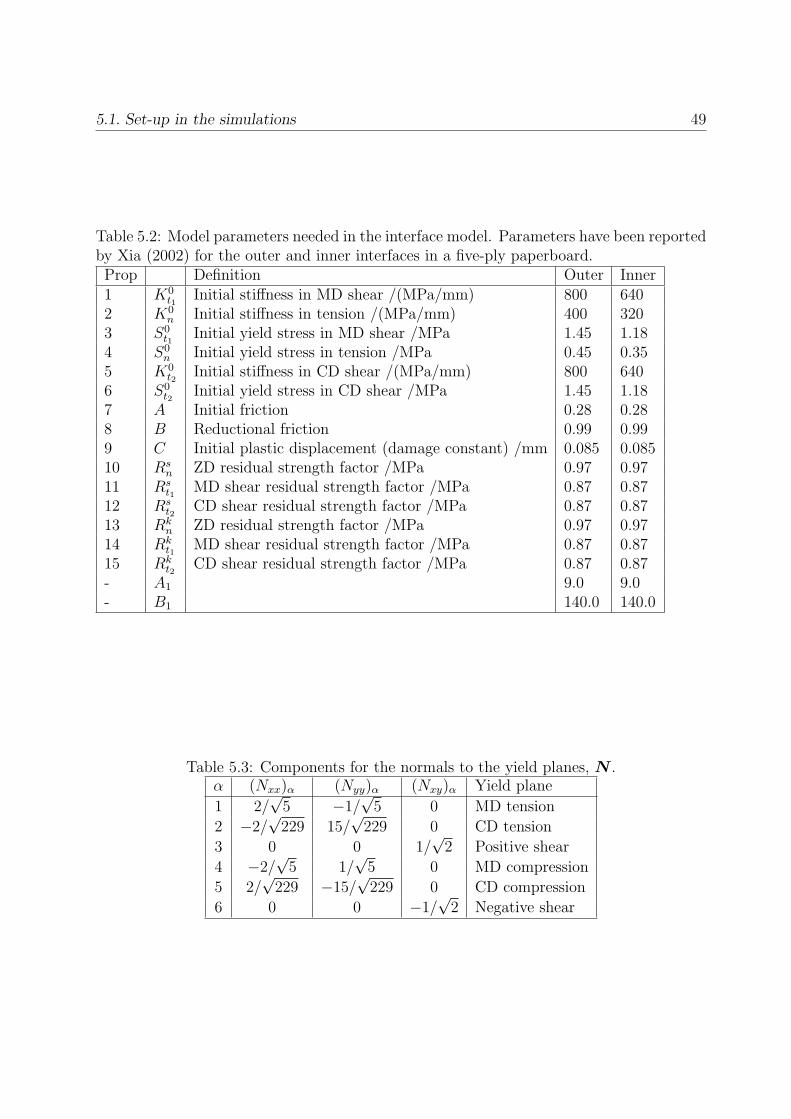
5.1. Set-up in the simulations 49
Table 5.2: Model parameters needed in the interface model. Parameters have been reportedby Xia (2002) for the outer and inner interfaces in a five-ply paperboard.Prop Definition Outer Inner1 K0
t1Initial stiffness in MD shear /(MPa/mm) 800 640
2 K0n Initial stiffness in tension /(MPa/mm) 400 320
3 S0t1
Initial yield stress in MD shear /MPa 1.45 1.184 S0
n Initial yield stress in tension /MPa 0.45 0.355 K0
t2Initial stiffness in CD shear /(MPa/mm) 800 640
6 S0t2
Initial yield stress in CD shear /MPa 1.45 1.187 A Initial friction 0.28 0.288 B Reductional friction 0.99 0.999 C Initial plastic displacement (damage constant) /mm 0.085 0.08510 Rs
n ZD residual strength factor /MPa 0.97 0.9711 Rs
t1MD shear residual strength factor /MPa 0.87 0.87
12 Rst2
CD shear residual strength factor /MPa 0.87 0.8713 Rk
n ZD residual strength factor /MPa 0.97 0.9714 Rk
t1MD shear residual strength factor /MPa 0.87 0.87
15 Rkt2
CD shear residual strength factor /MPa 0.87 0.87- A1 9.0 9.0- B1 140.0 140.0
Table 5.3: Components for the normals to the yield planes, N .α (Nxx)α (Nyy)α (Nxy)α Yield plane
1 2/√
5 −1/√
5 0 MD tension
2 −2/√
229 15/√
229 0 CD tension
3 0 0 1/√
2 Positive shear
4 −2/√
5 1/√
5 0 MD compression
5 2/√
229 −15/√
229 0 CD compression
6 0 0 −1/√
2 Negative shear

50 Chapter 5. Simulations and results
The reaction force and the displacement of the male die is measured according to figure5.3. In order to get comparable forces the reaction is multiplied with the width of the testpiece. The specimens used in the experiments had the width 38±1mm. The shape of themale and female die is described in figure 5.4. A web tension of 1000 N/m was applied tothe end of the paperboard and stoppers are located at the top of the paperboard accordingto figure 5.1. The stoppers where not included in the test equipment but was used in themodel to keep the paperboard in place. The stoppers and male die are assumed to befrictionless and the female die is assumed to have the friction coefficient 0.1.
Figure 5.1: Set-up in the simulations.
Figure 5.2: Material and interface properties.
5.2 Results
The simulations for the uniaxial tension and compression and pure shear, seen in figure 5.5to 5.7, is done for one gauss point in CALFEM/MATLAB. The code is the same as in theUMAT with small changes to fit the different notations.
In figure 5.8 and 5.9 the simulation of the crease is seen. In figure 5.8 the male die is in itsdeepest position and 5.9 is from the end of the process. The colours represent the differentvalues of the plastic strain in ZD compression.

5.2. Results 51
Figure 5.3: Definitions of the force acting on and displacements of the male die.
Figure 5.4: Measure of male- and female die in simulations.

52 Chapter 5. Simulations and results
(a) Four different curves for uniaxial compressionand tension.
(b) Uniaxial tension and subsequent compression.
(c) Two different curves for positive and negativeshear.
(d) Positive shear and subsequent negative shear.
Figure 5.5: Simulation of in-plane behaviour of mechanical plies of paperboard.

5.2. Results 53
(a) ZD-compression in subsequent loading and un-loading compared with model by Stenberg (2003).
(b) ZD-tension. Has only elastic behaviour.
Figure 5.6: Out-of-plane normal behaviour of continuum model.
(a) Two different curves for positive and negativeshear.
(b) Positive shear and subsequent negative shear.
Figure 5.7: Out-of-plane shear behaviour of continuum model.

54 Chapter 5. Simulations and results
Figure 5.8: Simulation of creasing of paperboard with male die in its deepest position.
Figure 5.9: Simulation of creasing of paperboard; end of procedure.

5.2. Results 55
Figure 5.10 shows the force-displacement curves for the male die. The different curvesrepresent experiment, simulation with the 3DM model with parameters from Xia (2002),simulation with the 3DM model with parameters from Nygards (2005) and simulation withthe model proposed in this thesis. The experimental data and the simulation with theparameters from Xia (2002) is obtained from Elison and Hansson (2005). The simulationset-up is the same in the simulation by Nygards (2005) and for the simulation with theproposed model. It is a slight difference between this set-up and the simulation set-up usedby Elison and Hansson (2005). Both set-ups are however built to resemble the experimentalset-up.
Figure 5.10: Force-displacement diagram for the male die in creasing.

56 Chapter 5. Simulations and results

Chapter 6
Discussion and conclusions
In figure 5.10 the result of the simulations is seen. The behaviour in unloading is better thanfor the original 3DM model. The out-of-plane shear parameters can be set to better capturethe initial part of the unloading but will then not give the accurate remaining deformation,or the parameters can be set to give the accurate remaining deformation but the unloadingcurve will then not be accurate. In other words the stiffness change during unloading inthe experiments seen in figure 5.10 can not be captured. From the results presented infigure 5.10 it can seem as if we get very good results, but it should be remembered thatthe out-of-plane shear components has not been experimentally determined, and we havefreedom to set these in order to capture the creasing procedure.
An advantage with the implementation of the proposed model is that the tolerance criteriaset by ABAQUS/Standard does not have to be changed due to convergence problems ashas been reported for the present implementation of the 3DM model (Elison and Hansson,2005). By not increasing these parameters causes the simulation curve to be smootherand more accurate than if the parameters are changed. That the implementation of theproposed model gives a smoother curve than for the present implementation of the 3DMmodel can be seen in figure 5.10.
The most important note to make about the model proposed is that it is a small deformationmodel. The model does not make a difference between the deformed configuration and theoriginal configuration, it solves the equations in the original configuration without mappingthe forces between the two states. This has the effect that the rigid body rotation in thecreasing procedure will cause stress in the paper. It is outside the scope of this workto incorporate large rotations, but it is believed that this can be done with (hopefully)relatively small efforts by letting the FE-software use co-rotated strains and stresses.
The three dimensional small deformation continuum model presented is this thesis is splitinto two uncoupled models; the in-plane model and the out-of-plane model. To do this,two assumptions has to be made. First, the two Poisson’s ratios coupled to the through-thickness directions are assumed to be zero, according to many investigations this does not
57

58 Chapter 6. Discussion and conclusions
seem to be far from the truth. Secondly, the in-plane behaviour is assumed not to dependon the out-of-plane deformations and vice versa. The second assumption is not evidentand it would to some extent be surprising if it holds, especially the high compressions thata creasing procedure causes could probably affect the in-plane behaviour.
As mentioned in a previous chapter the set-up is built up in a way that lets the paperalmost experience plain stress state. However, it would probably have been better to applyplain strain state to the paperboard or increase the width of the paperboard in the modelto get a simulation set-up with more close correlation to the experiments.
In a creasing procedure the three important components are the normal behaviour in ZD,one in-plane direction and the shear between these two directions. The continuum modelproposed by Xia (2002) has plasticity in the in-plane direction and only elasticity in thetwo remaining components. The interface model proposed by Xia (2002) separates thelayers of elements and incorporates remaining stresses between the layers and it can beargued that this will lead to remaining plasticity in the paperboard. However, this hasbeen examined by Elison and Hansson (2005) and as can be seen in figure 5.10 this doesnot lead to enough deformation after a crease. Therefore it is believed that a model, asthe one presented in this thesis, with plasticity in all components is important.
6.1 Further work
As mentioned earlier it is seen in figure 5.10 that the experiments during unloading hasa stiffness change i.e. an angle that can not be captured with the present model. Onereason for this could be that the elastic out-of-plane shear stiffness depends on the ZDcompression. To visualize this check figure 6.1. It could be that the paper in figure 6.1(b)is harder to shear, in order to give the same shear strain as in figure 6.1(a), since the fibresare more closely packed. If this holds it should be noted that it is not strictly true torefer to paper as an orthotropic material since, as can be seen in equation 3.6, there is nocoupling between normal strain and shear stress in orthotropic materials.
As mentioned in the previous section the in-plane model and the out-of-plane model areuncoupled. To fully examine this coupling in order to get the full yield surface, and theevolvement of it, for all components in the continuum model is very hard to do, but tostrive to do this would give much knowledge in order to build an accurate material model.
Elison and Hansson (2005) has shown in a parameter study that the interface parametersare ”very important”in the original 3DM model, and that even small changes of the interfaceparameters affect the result. It is believed that the interface model is as important in theproposed model as in the original 3DM model for the creasing operation. Not as importantas the relevant components in the continuum model but still important. Therefore, it is ofvital importance to calibrate the out-of-plane model in the continuum model together withthe interface model so that they together capture the relevant behaviour. It should also be

6.1. Further work 59
(a) Schematic of uncompressed fibres.
(b) Schematic of compressed fibres.
Figure 6.1: The effect that compressed fibers could have a larger shear stiffness than un-compressed fibres is not incorporated in the proposed model or in any orthotropic material.
noted that since the interface model is a traction-displacement based model the number ofinterfaces used in the simulations is important to consider when the models are calibrated.
It is, as mentioned earlier, important to add a model that controls the delamination sinceonly one continuum model can not capture this behaviour, but since the interface modelonly incorporates remaining stresses and separate the plies this may not damage the struc-ture enough during a creasing operation, to give the proper behaviour in the subsequentfolding. If it is shown that the structural weakening due to the separation of the pliesis not enough in the present models, one way of handling this could be to let the modelthat controls the delamination have a distribution in ZD according to figure 6.2. Whenthe delamination model weakens in the plastic region the elements will not be able to takeup load and the structure softens. This can be seen as the fibres that take part of thedelamination process and are unable to take up a substantial amount of load.
Figure 6.2: Proposal for a delamination model with distribution in ZD.
The in-plane model has isotropic hardening, i.e. it makes no difference between differenttypes of plastic strain. If experiments show that this does not hold, use can be made ofthe fact that the model is made up of several yield planes. Therefore, we can - insteadof adding kinematic or mixed hardening - couple extra plastic variables which evolve with

60 Chapter 6. Discussion and conclusions
and control the different yield planes.
In the in-plane model it is assumed that the flow is associated and in order to get the
plastic strain ratios correct (dεp
CD
dεMDfor MD tension and
dεpMD
dεCDfor CD tension) the shape of
the yield surface is changed. This coupling between the shape of the yield surface and theflow direction is not evident. And it is proposed that the experiments measured for thebiaxial failure surfaces are better as a ground for the shape of the yield surface than theplastic strain ratios. However, in order to uncouple the flow direction and the plastic strainratios from the shape of the yield surface a non-associate flow rule is required.
The present in-plane model relies on the assumption that the yield surface has the samecharacteristics as the, in experiments observed, failure surface. This is done since no yieldsurface for paper has been measured. Since the yield surface and the evolvement of itforms the ground in material models the biaxial yield surface for paper would be valuableto examine.
During this work data for the out-of-plane compression of paperboard was unavailable.Instead, the behaviour of the out-of-plane model in compression was fitted to the modelpresented by Stenberg (2003). The proposed model should be calibrated to fit experimentaldata.
Both the present implementation of the 3DM model Nygards (2005) and the model pre-sented in this thesis make use of fact that the theory presented by Xia (2002) has a sym-metric stress and strain tensor. This together with the fact that only three componentsare present in the in-plane model results in that we can use a vector with three compo-nents and engineering shear strain instead of the full second order tensor for the stress andstrain. This way the implementation becomes easier. However, in the implementation anextra factor 2 is required when summation convention is used. If instead the definitions arechanged to fit with engineering sheer strain and that the effective plastic strain is definedas εp
eff = ‖εpi ‖ this would have the advantages that; the implementation would be more
straight forward; the flow direction N could be normalized towards pure engineering shearstress at the same time as the parameters for the yield planes for shear, σIII
s , (SIII for largedeformations) take the same values as the yield stress in pure shear; the interpretation ofthe pure shear behaviour would fit to the use of engineering shear strain. This would how-ever be a change in the formulation of the theory and calibration of the shear componentswould have to be remade.
Additionally, a few other extensions can be added to incorporate other behaviour of thepaperboard.
• Fracture conditions.
• Strain rate effects, this opens up for the possibility to predict creep.
• Moisture dependence

Bibliography
ABAQUS (2004). ABAQUS User’s Manual. Hibbitt, Karlsson & Sorensen Inc, Pawtucket,RI, USA, 6.5 edition.
Arcan, M., Hashin, Z., and Voloshin, A. (1978). A method to produce uniform plane-stress states with application to fiber-reinforced materials. Experimental Mechanics,18(4):141–146.
Austrell, P. E., Dahlbom, O., Lindeman, J., Olsson, A., Olsson, K., Persson, K., Petersson,H., Ristinmaa, M., Sandberg, G., and Wernberg, P. A. (2004). CALFEM - A FiniteElement toolbox. The division of structural mechanics, Lund University, 3.4 edition.
Baumgarten, H. L. and Gottsching, L. (1973). Triaxial deformation of paper under tensileloading. In Proc. The fundamental properties of paper related to its uses, pages 227–249,Cambridge, England. The Brittish paper and board industry federation.
Belytschko, T., Liu, W. K., and Moran, B. (2000). Nonlinear finite elements for continuaand structures. John Wiley & Sons Ltd.
Carlsson, L., Ruvo, A. D., and Fellers, C. (1983). Bending properties of creased zones ofpaperboard related to interlaminar defects. Journal of Materials Science, 18:1365–1373.
deRuvo, A., Carlsson, L., and Fellers, C. (1980). The biaxial strength of paper. TAPPI,63:133–136.
Dunn, H. M. (2000). Micromechanics of paperboard deformation. Master’s thesis, Massa-chusetts institute of technology.
Elison, O. and Hansson, L. (2005). Evaluating the 3DM model - An experimental and finiteelement study. Master’s thesis, Department of mechanical engineering, Solid mechanics,Lund institute of technology.
Fellers, C. and Norman, B. (1998). Pappersteknik. Institutionen for Pappersteknik, KunglTekniska Hogskolan, Stockholm, third edition.
Fellers, C., Westerlind, B., and deRuvo, A. (1981). An investigation of the biaxial failureenvelope of paper. Proceeding of 7th Fundamental Research Symposium: The Role ofFundamental Research in Papermaking, pages 527–556.
61

62 BIBLIOGRAPHY
Gunderson, D. E. (1983). Determining paperboard strength. International Paper PhysicsConference, pages 253–263.
Hill, R. (1950). The mathematical theory of plasticity. Clarendon Press, Oxford.
Ohrn, O. E. (1965). Thickness variations of paper on stretching. Svensk Papperstidning,68(5):141–149.
Lagace, P. A. (2005). Equations of elasticity. Massachusetts Institute of Tech-nology, OpenCourseWare (http://ocw.mit.edu/NR/rdonlyres/Aeronautics-and-Astronautics/16-20Structural-MechanicsFall2002/891F16EA-EA88-4250-8AE5-1B3D6BA12511/0/unit4.pdf), 12/12 2005.
Mahnken, R. (1999). Aspects on the finite-element implementation of the gurson modelincluding parameter identification. International Journal of Plasticity, 15:1111–1137.
Mann, R., Baum, G., and Habeger, C. (1980). Determination of all nine orthotropic elasticconstants for machine-made paper. Tappi Journal, 63(2):163–166.
Nygards, M. (2005). 3DM - Three dimensional finite element modelling of paperboard.Technical Report no. 67, STFI-Packforsk.
Ortiz, M. and Popov, E. (1985). Accuracy and stability of integration algorithms forelastoplastic constitutive equations. International Journal for Numerical Methods inEngineering, 21:1561–1576.
Ottosen, N. and Petersson, H. (1992). Introduction to the Finite Element Method. PrenticeHall.
Ottosen, N. and Ristinmaa, M. (2005). The Mechanics of Constitutive Modeling. Elsevier,first edition.
Persson, K. (1991). Material model for paper. Master’s thesis, Lund institute of Technology,Lund, Sweden.
Ristinmaa, M. (2003). Review of plasticity model for paper and paperboard. Technicalreport, Division of Solid Mechanics, Lund University.
Stenberg, N. (2002a). On the out-of-plane mechanical behaviour of paper materials. PhDthesis, Royal Institute of Technology (KTH), Solid Mechanics.
Stenberg, N. (2002b). Out-of-plane shear of paperboard under high compressive loads.Journal of Pulp and Paper Science, 30(1):22–28.
Stenberg, N. (2003). A model for the through-thickness elastic-plastic behaviour of paper.International Journal of Solids and Structures, 40:7483–7498.
Stenberg, N. and Fellers, C. (2002). The out-of-plane poisson’s ratios of paper and paper-board. Nordic Pulp and Paper Research Journal, 17(4):387–394.

BIBLIOGRAPHY 63
Stenberg, N., Fellers, C., and Ostlund, S. (2001a). Measuring the stress-strain properties ofpaperboard in the thickness direction. Journal of pulp and paper science, 27(6):213–221.
Stenberg, N., Fellers, C., and Ostlund, S. (2001b). Plasticity in the thickness direction ofpaperboard under combined shear and normal loading. Journal of Engineering Materialsand Technology, 123:184–190.
Tsai, S. and Wu, E. (1971). A general theory of strength for anisotropic materials. Journalof Composite materials, 5:58–80.
Xia, Q. S. (2002). Mechanics of inelastic deformation and delamination in paperboard.PhD thesis, Massachusetts institute of technology.
Zienkiewicz, O. C. and Taylor, R. L. (2000). The finite element method. Butterworth-Heinemann, fifth edition.

64 BIBLIOGRAPHY

Appendix A
Comments to the model proposed byStenberg (2003)
It has been inside the scope of this master’s thesis to incorporate a model for the out-of-plane behaviour of the continuum model. A model formulated by Stenberg (2003) was firstimplemented, but two problems occurred that made the model unsuitable. Therefore, anew model has been developed and reported in this work. In this appendix the problemswith the model by Stenberg (2003) are described. Since another model is proposed in thisreport we will not go into details on the model, for further details cf. Stenberg (2003).
A.1 ZD compression
In this section the ZD compression of the model is reviewed. In the plastic region thismodel has two different solutions. One correct that follows the desired curve and onewhere the solution takes a wrong curve and the increment of the plastic multiplier (∆λ)takes negative values. The second solution is therefore clearly wrong. To have two differentsolutions where one is wrong is not unusual in numerical analysis and sometimes occur innumerical methods within constitutive modelling, reported before by Mahnken (1999). Theproblem in this model is instead that there is a jump for the right solution when goingfrom the elastic to the plastic region as can be seen in figure A.1. This causes considerableproblems when solving it numerically (and it is not the way the material would act). Infigure A.1 this behaviour is illustrated.
To further visualize this problem cf. figure A.2. Since we have implicit equations both forthe elastic region and the plastic region, the problem is solved numerically. The solutionprocedure is set up in the same manner as earlier with the solution reached when a function,F , reaches zero. This function is plotted in figure A.2 at the position when the solutiongoes from elastic to plastic response. We here see the two solutions for the plastic function
65

66 Chapter A. Comments to the model proposed by Stenberg (2003)
Figure A.1: ZD-compression in model proposed by Stenberg (2003).
where one coincides with the elastic function.
A.2 Shear model
Stenberg has measured the yield surface in a modified Arcan device (Stenberg et al., 2001b)and sheared it along the fibres according to figure A.3. The delamination between the fibreshas been measured and this shear behaviour is not suitable for the continuum model thatis supposed to capture the behaviour of the fibres. Figure A.4 shows the beginning ofplasticity in the out-of-plane shear components, with the different colours representing theout-of-plane shear stress. The hardening is described by a hyperbolic tangent-function thatreaches a plateau. The material can not take up more shear force when the top load isreached and the material deforms with ideal-plasticity, cf. figure A.5. The shear modelproposed by Stenberg (2003) is to some extent a delamination model.

A.2. Shear model 67
Figure A.2: The functions to solve for the plastic solution and the elastic solution in theboundary between plastic and elastic region.
Figure A.3: Principle of device used in measuring the out-of-plane shear behaviour.

68 Chapter A. Comments to the model proposed by Stenberg (2003)
Figure A.4: Beginning of plastic shear deformation in out-of-plane shear model proposedby Stenberg (2003).
Figure A.5: End of creasing in out-of-plane shear model proposed by Stenberg (2003).

Appendix B
Calculations used in theimplementation
B.1 In-plane model
In order to calculate the stress we need to solve equation (4.14) that for the in-plane modeltakes the form
F =
σ
(i)xx − σ?
xx + D1k∆λK(i)k
σ(i)yy − σ?
yy + D2k∆λK(i)k
σ(i)xy − σ?
xy + D3k∆λK(i)k∑n
I=1 χI
(σ
(i)i NI
i
σI(i)s
)2k
− 1
= 0. (B.1)
With the unknowns
x =
∆λ
σ(i)xx
σ(i)yy
σ(i)xy
. (B.2)
A factor 2 is required for the shear components due to the summation convention, this isfor convenience added in the vector N , hence
N =
Nxx
Nyy
2Nxy
. (B.3)
69

70 Chapter B. Calculations used in the implementation
Equation (B.1) is solved with the Newton-Raphson procedure described in equation (4.18).With the Jacobian
dFdx
=
∂F1
∂x1
∂F1
∂x2
∂F1
∂x3
∂F1
∂x4∂F2
∂x1. . .
∂F3
∂x1. . .
∂F4
∂x1. . .
, (B.4)
where the components are
∂Fi
∂x1
= Dik(Kk + ∆λ∂Kk
∂Kl
∂Kl
∂∆λ), (B.5)
∂Fi
∂xj+1
= δij + Dik∆λ(2k − 1)(2k)n∑
I=1
(σ : NI
σIs
)2k−2
χINI
k
(σIs)
2N I
j , (B.6)
∂F4
∂xi+1
= Ki (B.7)
and∂F4
∂x1
= −2kn∑
I=1
[(σ : NI)
2k
(σIs)
2k+1χI
(AIBItanh2(BI(∆λ + εp(n))) + CI
)]. (B.8)
These components contains
Ki = 2kn∑
I=1
(σ : NI
σIs
)2k−1
χINI
i
σIs
(B.9)
, (B.10)
∂Kk
∂Kl
=1
(K21 + K2
2 + K23)3/2
K22 + K2
3 −K1K2 −K1K3
−K1K2 K21 + K2
3 −K2K3
−K1K3 −K2K3 K21 + K2
2
, (B.11)
∂Kk
∂∆λ= −2k ∗ 2k
n∑I=1
(σ : NI)2k−1
(σIs)
2k+1χIN
Ik
∂σIs
∂∆λ(B.12)
and∂σα
s
∂∆λ= AαBαtanh2(Bα(∆λ + εp(n))) + Cα. (B.13)
In order to use the Newton-Raphson method a start guess is required. The start guessdoes not influence the result (if obtained), only the number of iterations required to achieveconvergence. The start guess is taken as
x =
0
σ?xx
σ?yy
σ?xy
. (B.14)

B.2. Out-of-plane normal model 71
B.1.1 Material tangent stiffness components
In order to calculate the consistent material tangent stiffness the following matrix is re-quired
∂F∂ε
= −
D11 D12 D13
D21 D22 D23
D31 D32 D33
0 0 0
. (B.15)
B.2 Out-of-plane normal model
The elastic behaviour is described by the explicit equation
σzz = σtz
(1− exp
[1 + rorig
µ(exp[εp
zz]− exp[εzz])
]). (B.16)
The plasticity is described by
F =
[σzz − σt
z
(1− exp
[1+rorig
µ(exp[εp
zz −∆λ]− exp[εzz])])
= 0
σa(∆λ)− σ = 0
]. (B.17)
The unknowns are
x =
[σzz
∆λ
]. (B.18)
The required jacobian dFdx
has the components
∂F1
∂x1
= 1, (B.19)
∂F2
∂x1
= −1, (B.20)
∂F2
∂x2
= BσCσexp[−Cσ(εpzz −∆λ)], (B.21)
and
∂F1
∂x2
= −σtz
rorig + 1
µ
(1− exp
[1 + rorig
µ(exp[εp
zz −∆λ]− exp[εzz]) + (εpzz −∆λ)
]).
(B.22)Since the model only contains one component and that if plasticity occurs it will occur inthat component, it is believed that it is a better assumption, for the start guess, that theentire step is plastic and the start guess is taken as
x =
[σ?
zz
∆εzz
]. (B.23)

72 Chapter B. Calculations used in the implementation
B.2.1 Material tangent stiffness components
The required matrix is
∂F∂εzz
=
[−σt
zrorig+1
µexp[
1+rorig
µ(exp[εp
zz −∆λ]− exp[εzz]) + εzz
]0
]. (B.24)
B.3 Out-of-plane shear model
It should be noted that the components presented in this section is not used in the UMAT,instead a more complex way is used to implement the shear components, but it is (strongly)believed that they give the same result and that the presented components would have givena simpler implementation.
In this section the subscript i, j, k and l takes the 1 (corresponding to xz) and 2 (corre-sponding to yz). For the out of plane shear components the system to solve is
F =
σ(i)xz − σ?
xz + D1k∆λK(i)k
σ(i)yz − σ?
yz + D2k∆λK(i)k√
σ2xz + σ2
xz − τs(∆λ)
= 0, (B.25)
where
K(i)k =
∂f∂σ∥∥ ∂f∂σ
∥∥ (B.26)
and∂f
∂σk
=σk
‖σ‖. (B.27)
The unknowns are
x =
∆λ
σ(i)xz
σ(i)yz
. (B.28)
The required Jacobian has the components
∂Fi
∂x1
= DikKk, (B.29)
∂F3
∂x1
= −BτCτ tanh2(Cτ (γpeff + x1)), (B.30)
F3
xi+1
= Ki (B.31)

B.3. Out-of-plane shear model 73
and∂Fi
∂xi+1
= δij + Dik∆λ∂Kk
∂Kl
∂Kl
∂xi+1
. (B.32)
With∂Kk
∂Kl
=1
(K21 + K2
2)3/2
(K2
2 −K1K2
−K1K2 K21
)(B.33)
and∂Kl
∂xi+1
=1
(σ21 + σ2
2)3/2
(σ2
2 −σ1σ2
−σ1σ2 σ21
). (B.34)
The start guess is taken as
x =
0σ?
xz
σ?yz
. (B.35)
B.3.1 Material tangent stiffness components
The required matrix is∂F∂ε
= −[
Gxz 00 Gyz
]. (B.36)