A slip factor calculation in centrifugal impellers based on linear cascade data
21
A slip factor calculation in centrifugal impellers based on linear cascade data Dr. Abraham Frenk Becker Turbo System Engineering (2005). (Presented by Dr. E. Shalman)
description
This file is about compressor's blade.
Transcript of A slip factor calculation in centrifugal impellers based on linear cascade data

A slip factor calculation in centrifugal impellers based on
linear cascade data
Dr. Abraham FrenkBecker Turbo System Engineering (2005).
(Presented by Dr. E. Shalman)

AbstractAccurate modeling of the flow slip against direction of rotation is essential for correct prediction of the centrifugal impeller performance. The process is characterized by a slip factor. Most correlations available for calculation of the slip factor use parameters characterizing basic impeller geometry (review of Wiesner (1967) and Backstrom (2006)).
Approach presented below is based on reduction of radial cascade to equivalent linear cascade. The reduction allows to calculate characteristics of radial blade row using well established experimental data obtained for linear cascades, diffusers and axial blade rows.
2

Rotors with splitters or with high loading must be divided into few radial blade rows. In the case of multiple rotor blade rows the slip angle is calculated for each blade row. The slip angle of the rotor is a sum of the slip angles obtained for each row. Suggested reduction of radial blade rows allows also calculating of other parameters essential for impeller design.
Suggested method allows also determine additional causes influencing slip factor. The slip factor depends not only on parameters characterizing basic impeller geometry, but on difference of inlet flow angle from stall flow angle. In the rotors with the same basic geometry parameters slip factor depends on the length of the blade. Slip factor increases with blade length.
3

Axial compressor Centrifugal compressor4

ZRv ks 22 sinβπθ Ω=
Zk2sin
1βπ
σ −=
2k
Ca2
Cu2
C2
Stodola (1927)Busemann (1928) called this displacement flow; other authors refer to its rotating cells as relative eddies.
(definition)2
1R
v s
Ω−= θσ
5Slip flow in Centrifugal compressor

Axial compressor Centrifugal compressor
t
( ) ( )( )kka
u
c22
2
2 tantan1 βδβσ −+−=
7.02sin
1Z
kβσ −=
( ) ( )( ) tx kf θδβδ ++= 22 002.0223.0
(Wiesner)
Deviation angle δ = β2 - β2k.
Slip factor σ or slip angle δ = β2 - β2k.
Xf
Howell (1945)
6
Z-number of blades
Ca
Cu
2k
2
1
2211
12
−=
∆w
w
w
P
ρ
General Inviscid
( )( )
2
,2
,1
2
1
2211 cos
cos11
2
−=
−=
∆
eqv
eqveqv
w
w
w
P
ββ
ρ
In Linear cascade Ca1= Ca2
General blade row
( )( )
2
2
1
2
1
2211 cos
cos11
2
−=
−=
∆DK
w
w
w
P
ββ
ρ
Equivalent linear cascade∆P = ∆Peqvβ2 =β2,eqv
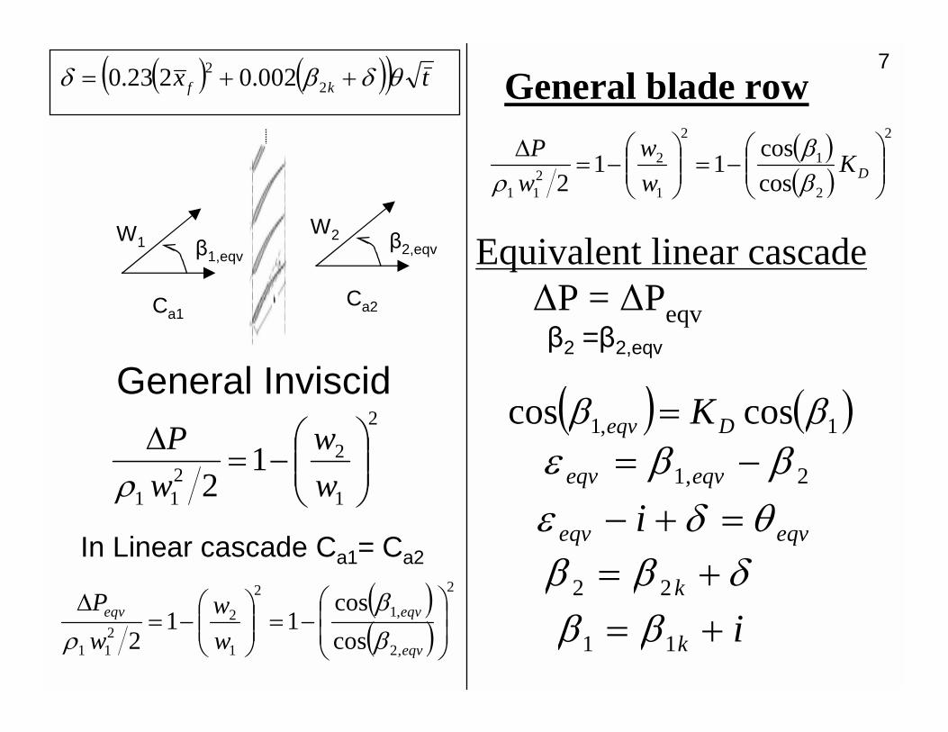
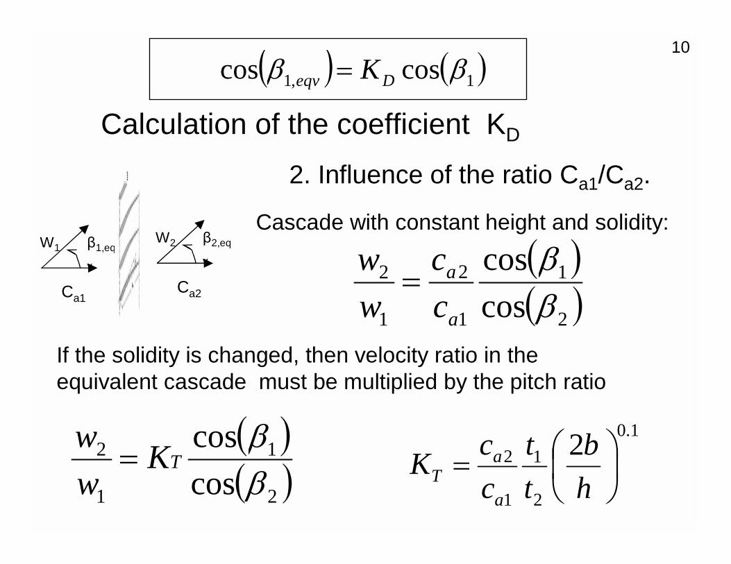
( ) ( )1,1 coscos ββ Deqv K=
2,1 ββε −= eqveqv
eqveqv i θδε =+−
( ) ( )( ) tx kf θδβδ ++= 22 002.0223.0
δββ += k22
ik += 11 ββ
W2
Ca2
β2,eqvW1
Ca1
β1,eqv
7

b
Calculation of equivalent pitch (solidity)
( ) ( )( ) ( )1002.0223.0 22
2,2 −+++= eqveqvkfkeqvk tx θδβββ
( ) ( )( ) eqveqvkfeqv tx θδβδ ++= 22 002.0223.0
( ) ( )21
22
121
22 22
tt
t
b
t
btt
tteqv +
=+
=
8
( ) ( )( )eqvkeqveqvka
u
c,2,2
2
2 tantan1 βδβσ −+−=

( )( )
1.0
212
12 2
/
/
=
= h
b
ww
ww
bh
Experimental data for diffusers
1. Influence of the channel height h.
Calculation of the coefficient KD
Stratford (1959) obtained the height (h) of the diffuser with given length (b) that has maximal static pressure rise coefficient. The velocity ratio w2/w1 depends on the ratio b/h. The experimental data for linear cascade were obtained for h=2b. The experimental data of Stafford may be approximated by equation
( ) ( )1,1 coscos ββ Deqv K=9
2. Influence of the ratio Ca1/Ca2.
Calculation of the coefficient KD
( )( )2
1
1
2
1
2
cos
cos
ββ
a
a
c
c
w
w=
Cascade with constant height and solidity:
1.0
2
1
1
2 2
=
h
b
t
t
c
cK
a
aT
If the solidity is changed, then velocity ratio in the equivalent cascade must be multiplied by the pitch ratio
( )( )2
1
1
2
cos
cos
ββ
TKw
w=
W2
Ca2
β2,eq
v
W1
Ca1
β1,eq
v
( ) ( )1,1 coscos ββ Deqv K=10
Calculation of the coefficient KD
( )( )
( )( )2
1
,2
,1
1
2
cos
cos
cos
cos
ββ
ββ
T
eqv
eqv Kw
w==
For axial compressors
TKTD KK 2
1
=
Hence, KT=KD
In General case 1.0
2
1
1
2 2
=
h
b
t
t
c
cK
a
aTwhere
W2
Ca2
β2,eq
v
W1
Ca1
β1,eq
v
( ) ( )1,1 coscos ββ Deqv K=11
(effect of boundary layer separation and blockage)
1.0
2
1
1
2 2
=
h
b
t
t
c
cK
a
aT
where

The rotor with splitters is divided into sequence of rotors. Each rotor has the same number of blades at inlet and exit.
For high loaded rotors the loading of each equivalent linear cascade must be less then maximal allowed.
12
Impellers with high blade loading and splitters

Calculate slip anglefor each rotor.
The slip angle of the rotor is a sum of the slip angles obtained for each row
Rotor 1
Rotor 2
13
Impellers with high blade loading and splitters

14
( ) ( )1,1 coscos ββ Deqv K=
High blade loading
Stall conditions
TKTD KK 2
1
=1.0
2
1
1
2 2
=
h
b
t
t
c
cK
a
aT

Maximal pressure gradient
( )( ) tmw
w
w
P
ststeqv
steqv
st
stst
+=
−=
−=
∆1
124.1
cos
cos11
2
2
,2
,1
2
,1
,2211 β
βρ
Analysis of experimental data of Howell (1945), Emery (1957), Bunimovich (1967)allows obtaining following equation for coefficient of static pressure rise at stall conditions (maximalpressure rise)
Parameter mst characterizes type of the cascade. E.g. For cascades studied by Howell mst =1.
btt /= is relative pitch of the linear cascade
( ) ( )∫∫ −−=b
essureSide
b
eSuctionSidst dbwwdbwwm0
Pr1
0
1
15
( ) ( )1,1 coscos ββ Deqv K= TKTD KK 2
1
=1.0
2
1
1
2 2
=
h
b
t
t
c
cK
a
aT

1. Stage of turbojet Olympus 2. Stage tested by Stechkin3. Stage designed by Beker Engineering and tested at
Concept. 4. Stage designed by Beker Engineering , not tested5. Stage C1 (tandem blades) (data from USSR) 6. Monig et al. Trans ASME. Journal of turbomachinery
1993,v115, p.565-571. 7. Stage C9 (data from USSR) 8. Musgrave D., Plehn N.J. Mixed flow stage design and test
results with a pressure ratio of 3:1. ASME Gas turbine conference presentation 87-GT-20.
Compressor Stages used to test the model
16

Results
510.616560.050.6121.01.7819.92.896.3612/248
52016146.250.1750.562.186.252.756.7918/367
42516050.470.3160.742.08.482.03.8615/306
455185.346.650.3460.252.129.02.74.5427/275
550182.956.330.6411.502.148.281.03.877/144
500189.357.480.3971.271.8912.00.485.2311/223
48317032.7-0.502.3033.583.03.95122
472.318057.80.6951.01.8316.990.414.356/121
u2
m/s(tip
velocity)
ca2
m/s
β1
(inlet
flow
angle )
t2,mean(outlet relative
pitch)
t1,mean(inlet relative
pitch)
β2k(outlet blade
angle)
G
Kg/s
Rotorpressure
ratio
Znumber
of blades
Rotor
No.
Table 1. Rotor parameters.
1
2
r
r
17

ResultsTable 2. Slip factor and exit angle.
0.8770.8610.8870.8950.8900.89335.035.98
0.9260.9310.9100.9190.9340.93317.817.97
0.8960.9140.8900.9080.8960.89923.023.326
0.9030.9100.8760.9020.9010.91520.620.175
0.8700.8340.7620.8740.875-56.3-4
0.8650.8800.8480.8880.8880.88727.027.03
0.8400.8230.720.8400.896-43.8-2
0.7840.7180.8600.8320.8780.88132.031.81
σEck
σStechkin
σStodola
σWiesner
σPresent
work
σmeasured
β2Present
work
β2
measured
Rotor
No.
18

Measured and calculated slip factor for 6 impellers
19

Calculated slip factor for 8 impellers
20

Conclusions• Suggested method allowing reduction of
arbitrary rotor blade passage to equivalent linear cascade
• Method allows establishing equivalence between axial and centrifugal impellers
• Method allows calculating slip factor based on well established linear cascade correlations for deviation angle
21