A SIMULINK MODEL FOR SIMULATION OF OPTICAL
47
Department of Electrical and Computer Systems Engineering Technical Report MECSE-31-2004 A SIMULINK Model for Simulation of Optical Communication Systems: Part I – Single Channel Transmission LN Binh and Jay Armstrong
-
Upload
kiranpataballa -
Category
Documents
-
view
1.881 -
download
5
description
A SIMULINK MODEL FOR SIMULATION OF OPTICALCOMMUNICATIONS SYSTEMS: PART I – SINGLE-CHANNELTRANSMSSION
Transcript of A SIMULINK MODEL FOR SIMULATION OF OPTICAL

Department of Electricaland
Computer Systems Engineering
Technical ReportMECSE-31-2004
A SIMULINK Model for Simulation of Optical CommunicationSystems: Part I – Single Channel Transmission
LN Binh and Jay Armstrong

1
The SIMULINK Optical Simulator - Fibre Optic Transmission Systems
A SIMULINK MODEL FOR SIMULATION OF OPTICAL
COMMUNICATIONS SYSTEMS: PART I – SINGLE-CHANNEL
TRANSMSSION
L.N. Binh and Jay Armstrong
Department of Electrical and Computer Systems Engineering, Monash university, Clayton
Victoria 3168 Australia, e-mail: [email protected]
Abstract
Optical communications have advanced tremendously over the last two decades, especially when
optical amplifiers were invented in the late 80s. Advances in optical communications systems
have been demonstrated in practice including a number of commercialised simulation packages.
However no complete simulation package has been developed under MATLAB Simulink platform
that are readily available and popular in engineering systems, especially as a teaching tool. This
report aims to investigate the various issues currently plaguing physical implementation of
optical transmission systems utilizing super dense channel spacing (SDWDM) at a bit rate
approaching 40 Gb/s under the SIMULINK optical simulator, for advanced optical
communications systems. Dispersion and carrier chirp effects are explored. The benefits of a
chirped transmission system have also been exploited. Signal propagation through n external
optical modulator, the optical fiber. Based in the MATLAB Simulink, the simulator simplifies the
simulation blocks of advanced optical transmission system.
MECSE-31-2004: "A SIMULINK Model for Simulation of Optical Communication ...", LN Binh and Jay Armstrong

2
The SIMULINK Optical Simulator - Fibre Optic Transmission Systems
TABLE OF CONTENTS
1 INTRODUCTION ................................................................................................................................................ 3 2 Overview of System Components ........................................................................................................................ 4
2.1 Receiver Noise Sensitivity:........................................................................................................................ 4 2.2 Optical fibers ............................................................................................................................................. 4 2.3 Optical Transmitters .................................................................................................................................. 5 2.4 Dispersion.................................................................................................................................................. 6 2.5 Polarization Mode Dispersion ................................................................................................................... 7 2.6 Carrier Chirp.............................................................................................................................................. 8 2.7 The Mach Zehnder Interferometric Modulator.......................................................................................... 8 2.8 Data Sampling ......................................................................................................................................... 11
3 THE SIMULINK© SIMULATOR...................................................................................................................... 11 3.1 Assumptions ............................................................................................................................................ 13 3.2 Data sampling .......................................................................................................................................... 14 3.3 The carrier................................................................................................................................................ 14 3.4 Data pulses............................................................................................................................................... 15 3.5 Equipment................................................................................................................................................ 15 3.6 System Initialization ................................................................................................................................ 16 3.7 Generating data streams and carriers ....................................................................................................... 16 3.8 The data random-bit-pattern pulse trains ................................................................................................. 17 3.9 Carrier Modulation .................................................................................................................................. 17 3.10 The split step propagation model............................................................................................................. 20 3.11 Dispersion as a Low Pass Filter ............................................................................................................... 24 3.12 The linear delay ....................................................................................................................................... 25 3.13 PMD as a Filter........................................................................................................................................ 27 3.14 Non-Linear Operator ............................................................................................................................... 28
4 The Simulator and a Case Study......................................................................................................................... 32 5 CONCLUDING REMARKS.............................................................................................................................. 42 6 References........................................................................................................................................................... 44 7 APPENDIX......................................................................................................................................................... 45
TABLE OF FIGURES
Figure 1: SIMULINK Block Diagram of the Simulator ............................................................................................. 12 Figure 2: Data Stream block sub system..................................................................................................................... 19 Figure 3 The Fibre split stp Fourier propagation model ............................................................................................. 22 Figure 4: Plot of the fibre delay term as a function of u ............................................................................................. 26 Figure 5: Non-linear effects model ............................................................................................................................. 31 Figure 6 : Initializing the simulator ............................................................................................................................ 34 Figure 7: Sample screen shot of the SIMULINK simulator....................................................................................... 34 Figure 8: (a)-(e) 5mW simulation – Non-linear effects negligible, N=1 .................................................................... 39 Figure 9: 50mW case – Non-linear effects, N=0.429 ................................................................................................. 41 Figure 10: Comparison of modulator output and fiber outputs for an input power of 5mW ...................................... 42
MECSE-31-2004: "A SIMULINK Model for Simulation of Optical Communication ...", LN Binh and Jay Armstrong

3
The SIMULINK Optical Simulator - Fibre Optic Transmission Systems
1 INTRODUCTION Over the last twenty years it has been witnessed the realization of low cost, low loss optical
fibers. Superior information capacity and versatility has seen optical fibers become the preferred
medium for modern long-haul ultra-high speed communication systems [1] However, the ever-
constant desire to increase data transmission rates requires further research to fulfill the potential
of fiber optic systems, in particular the flexibility of upgrading a particular wavelength channel
from 10 Gb/s, say to 40 Gb/s.
As material developments plateau, focus shifts from materials to transmission properties; a desire
to understand the propagation effect of fiber optics, as well as the transmission characteristics of
optical signals. It is anticipated that optimizing the various linear and non-linear effects present
in modern optical transmission systems and their optical-electrical (O/E) components would lead
to further developments in data transmission rates. This report aims to develop and simplify the
optical transmission system. Of particular interest were the effects of dispersion and polarisation
mode dispersion, the two single critical effects limiting the optical data transmission rates[2].
This work has led to the development of a visual based, modeling platform, using MATLAB
Simulink. This platform models signal propagation through a modern optical transmission
system with the modeling of the fiber propagation through the split step method. It is anticipated
that this platform will be a valuable tool for further research into different optical systems This
understanding can in turn be applied to optimize the performance of systems already being
installed. Through detailed research into physical limitations, means of measuring and
optimizing systems will become apparent. In particular this work aims to investigate the various
issues currently plaguing physical implementation of optical transmission systems operating of
the super dense WDM (SDWDM) at transmission rate in excess of 40Gb/s.
MECSE-31-2004: "A SIMULINK Model for Simulation of Optical Communication ...", LN Binh and Jay Armstrong

4
The SIMULINK Optical Simulator - Fibre Optic Transmission Systems
2 Overview of System Components In general an optical communications would consist of optical sources and modulators,
multiplexers, fiber, receivers and transmitters The following sections outline the major
components of a general optical transmission system. An explanation of their operation is given
as well as their role within a simulator. Various limiting parameters associated with each
photonic or optoelectronic device are also introduced.
2.1 Receiver Noise Sensitivity: Initially receivers were considered and in particular the effects of noise relative to their
sensitivity. It is determined that the noises accumulated in photo-detectors are of three distinct
types: (i) Laser intensity noise: Primarily caused due to spontaneous light emissions occurring in
the transmitter.(ii) Thermal noise: A result of connecting electronic components to the
receiver.(iii) Photonic quantum shot noise: a result of the quantum nature of photons.
Thermal noise can be reduced if the transfer impedance can be increased, but this would reduce
its effective bandwidth. Essentially low noise amplifiers are connected to the photo diode, if a
narrow bandwidth amplifier then only a few decibels (dB) of noise should be present. Middle
bandwidth amplifiers would incorporate about 6-8dB of noise, and high frequency amplifiers
should cause less than 15dB of noise. Shot noise is simply reduced by reducing the intensity of
the light that is transmitted. Similarly, applying various filters will limit reflections back into the
laser source and reduce laser intensity noise. As receiver noise is controllable through already
known methods [[2[16] but it is not a major focus of this paper.
2.2 Optical fibers Apparently named single mode fibers (SMF), they are designed so as to maintain an optical
signal integrity for as long as possible. This gives single mode fibers incredible data capacity at
MECSE-31-2004: "A SIMULINK Model for Simulation of Optical Communication ...", LN Binh and Jay Armstrong

5
The SIMULINK Optical Simulator - Fibre Optic Transmission Systems
very low losses, lending them too many various applications. As a result, the standard SMF (ITU
G.652)have become the primary means through which data is transmitted. Further advanced
optical fibres can also be used such as NZ-DSF, Corning LEAF etc. with large effective index
area to maximize the channel input optical power. The dispersion of the transmission medium
can also be compensated using various dispersion compensating or management schemes.
2.3 Optical Transmitters In designing any fiber optic system one must decide how the electrical data signal can be
converted into an optical bit stream. For a system designer a number of options exist. Usually,
the output of an optical source, such as a semiconductor laser, is modulated through the
application of an electrical signal. Direct application of this current to control the laser gives rise
to the term direct modulation; conversely external modulation utilizes a separate photonic
device, such as the Mach-Zhender Interferometric modulator (MZIM), to control the optical
intensity pulse output. This gives rise to the two modulation formats, non-return to zero (NRZ)
and return to zero (RZ). If the RZ method is used, then the optical pulse used to represent one bit
is shorter than the allocated time slot for the bit, also known as the bit duration.
Before the completion of the bit duration the optical pulse returns to its zero value. In the NRZ
format the pulse does not automatically return to zero. Rather the optical pulse remains on until
the end of the bit duration. This means that the pulse widths in a NRZ format can vary according
to the bit stream being transmitted. On/off transitions occur less regularly in the NRZ format
therefore reducing the bandwidth associated with a particular bit stream. This is usually by a
factor of about two. This smaller bandwidth leads to NRZ often being the format of choice in
data transmission systems.
The optical carrier waveform generated by a CW operating laser source before modulation is
usually represented by:
MECSE-31-2004: "A SIMULINK Model for Simulation of Optical Communication ...", LN Binh and Jay Armstrong
6
The SIMULINK Optical Simulator - Fibre Optic Transmission Systems
C(t)=A cos(ω0t+φ) (eq. 1)
where A is the amplitude of the optical signal envelop, ω0 is the carrier frequency and φ is the
carrier phase [1[16] Any of these parameters can be used as variables for modulating electrical
signal to optical domain. The MZIM as illustrated later utilizes a phase shift to induce amplitude
modulation.
2.4 Dispersion In IM/DD systems, usually operating at less than 2.5 Gb/s, the dispersion had not been a major
issue owing to the rather widely spaced channels used. However for higher bit-rate systems (>10
Gb/s) incorporating DWDM require an increased density in channel spacing. As a result
dispersion has become a very important issue. This causes inter-symbol interference at the
receiver increasing bit-error rates (BER), eventually rendering the signal unrecognizable. Figure
4 illustrates this dispersion issue and the occurrence of cross talk in faster systems utilizing
DWDM.
Chromatic dispersion is defined as being the spreading/broadening of transmitted data pulses as a
function of the group velocity of different optical frequencies. In advanced systems employing
multiplexed channel and narrow channel spacing, the compensation method would not
sufficiently overcome the problem of dispersion. In fact dispersion effects have come to be the
single biggest limiting factor in such ultra-long reach optical communications systems. The
effects of dispersion are directly related to the speed of transmission. Thus ultra-high speed
systems are more greatly affected by dispersion that occurs as a result of two major factors: (i)
Different wavelengths in DWDM systems: channel transmission utilizes different wavelengths to
send data. This causes slight variations in the refractive index of optic fiber causing signal
dispersion; and (ii) The transmitter: ‘chirp’ induced by the laser modulator will cause dispersion
by slightly varying the carrier frequency, altering the refractive index of the fiber.
MECSE-31-2004: "A SIMULINK Model for Simulation of Optical Communication ...", LN Binh and Jay Armstrong

7
The SIMULINK Optical Simulator - Fibre Optic Transmission Systems
If ∆ω represents the spectral width of an optical pulse it can be shown that the pulse dispersion
over a length of fiber L is given by:
∆T=Lβ2∆ω
(eq. 2)
where β2 is known as the GVD parameter. It is this parameter that primarily determines the
broadening of a pulse as it propagates through an optical fiber. Sometimes ((eq. 2) can be
rewritten to consider the range of wavelengths that are emitted by the optical source. Defined as
dispersion this relation is given by:
D=-2πcβ2/λ2 (eq. 3)
where the dispersion is expressed in ps/nm.km, λ is the light wavelength and c is the speed of
light. Both of the aforementioned causes were considered before it was decided to focus on the
‘chirp’ effect. This was directly related on the desire to optimize current systems rather than
attempt to generate a whole new means of transmission.
2.5 Polarization Mode Dispersion Practical optical fibers are inherently asymmetric on account of the non-perfect conditions of
their drawing. As a result, light waves in one polarization axis can move at different speeds to
those in the other polarization axis. The effects of this delay become more critical at faster
transmission speeds. The varying speed causes delay in transmitted pulses. At higher
transmission rates this can cause signals to overlap, becoming indistinguishable at the receiver.
To quantify this occurrence the differential group delay (DGD) is defined as∆τ. Existing
statistical models make use of a Maxwellian distribution for the consideration of PMD effects.
From the statistical relationship a mean value can be determined and is used to quantify a fiber’s
PMD. This is represented by δτ and measured in units of ps/√km. [[15,[7]
MECSE-31-2004: "A SIMULINK Model for Simulation of Optical Communication ...", LN Binh and Jay Armstrong

8
The SIMULINK Optical Simulator - Fibre Optic Transmission Systems
2.6 Carrier Chirp With chirp found to be a major player in the cause of dispersion this parameter became a focus
for the project. If the chirp induced by the system transmitter could be minimized then so to
might the dispersion and thus the overall system performance. To achieve these goal two areas
need to be considered. Firstly the chirp causes impairments to other parameters in an optical
transmission system. Secondly, the actual mechanism of signal transmission, that is the
modulator. This paper will focus on the Mach-Zehnder interferrometric modulator on account of
its regular use in industry and its presence in the university optics laboratory. It was the
developed understanding of the chirp parameter and its effects on system performance that led to
the decision to simulate a modern fiber optic system using Simulink and will be discussed in
greater detail in later stages of this writing.
2.7 The Mach Zehnder Interferometric Modulator As previously mentioned dispersion was determined to be the major limiting factor in optical
systems. Further to this point it was found that the single biggest contributing factor to signal
dispersion was transmitter chirp. Paramount to an understanding of chirp is a need to understand
the technical operation of the system transmitter. This paper focuses on the Mach-Zehnder
Interferrometric Modulator (MZIM) on account of its popular use in practical systems.
The MZIM is a device that uses double side-band amplitude modulation (DSB AM) to transmit
data as a stream of optical pulses. It is an externally modulating system ideally suited to high-
speed data transmission on account of its narrow line-width. Figure 6 illustrates the topology of a
MZIM. It should be noted that figure 6 depicts a single electrode model. Also available is a dual
electrode device but the principles behind its operation remaining the same. This paper focuses
primarily on the single arm model.
MECSE-31-2004: "A SIMULINK Model for Simulation of Optical Communication ...", LN Binh and Jay Armstrong

9
The SIMULINK Optical Simulator - Fibre Optic Transmission Systems
The MZIM makes use of a titanium diffused LiNbO3 wave-guide in an interferometric
configuration. By applying an external voltage the refractive index of electro-optic materials can
change. This can be used to alter the phase of one of the optical paths. When the two paths merge
at the output of the modulator the two waveforms interfere with one another. In the absence of a
voltage, that is in the ‘On state.’ The phase of both carriers is equal, thus as they emerge from the
modulator constructive interference occurs generating a signal. In the ‘Off state’ a voltage is
applied to the electro-optical material, in this case LiNbO3. This causes modulation to the carrier
in the modulated guide, changing its phase. A change of 180 degrees in phase will cause
destructive interference that will cancel the two carriers as they recombine. This eradicates the
waves generating on ‘off’ signal [[8[9[10[11[12[13[14]. Thus, by driving the electrode by the data
stream to be transmitted one can control whether constructive or destructive interference occurs
allowing the electronic data stream to be converted into an optical signal. Unfortunately, it is not
possible to instantly change the phase delay of the modulator arms, which leads to the occurrence
of chirp. Rather the phase delay generated by the electrode changes transiently. Thus the chirp
for the single electrode MZIM can be found from the output electric field of the MZIM. The
output electric field o the lightwaves is given as
21
21
0θθ τ jj eeEE +=
(eq. 4)
where φ1 and φ2 represent the phase changes in arms 1 and 2 respectively. τ is a scaling factor
between 1 and 0 accounting for the particular geometry of the device being analyzed. A value
less than 1 denoting a power split not 50/50 between the two arms can be found from:
)1()1(
2/1
2/1
+−
=εετ
(eq. 5)
MECSE-31-2004: "A SIMULINK Model for Simulation of Optical Communication ...", LN Binh and Jay Armstrong
10
The SIMULINK Optical Simulator - Fibre Optic Transmission Systems
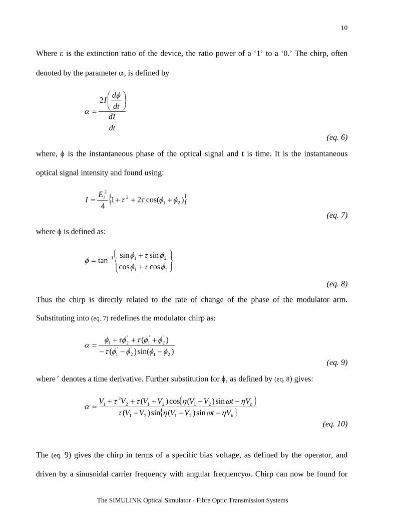
Where ε is the extinction ratio of the device, the ratio power of a ‘1’ to a ‘0.’ The chirp, often
denoted by the parameter α, is defined by
dtdI
dtdI ⎟
⎠⎞
⎜⎝⎛
=
φ
α2
(eq. 6)
where, φ is the instantaneous phase of the optical signal and t is time. It is the instantaneous
optical signal intensity and found using:
)cos(214 21
22
φφττ +++= iEI
(eq. 7)
where φ is defined as:
⎩⎨⎧
⎭⎬⎫
++
= −
21
211
coscossinsintan
φτφφτφ
φ
(eq. 8)
Thus the chirp is directly related to the rate of change of the phase of the modulator arm.
Substituting into (eq. 7) redefines the modulator chirp as:
)sin()()(
21'2
'1
'2
'1
'21
φφφφτφφττφφ
α−−−
+++=
(eq. 9)
where ′ denotes a time derivative. Further substitution for φ, as defined by (eq. 8) gives:
b
b
VtVVVVVtVVVVVV
ηωητηωηττ
α−−−
−−+++=
sin)(sin)(sin)(cos)(
2121
212122
1
(eq. 10)
The (eq. 9) gives the chirp in terms of a specific bias voltage, as defined by the operator, and
driven by a sinusoidal carrier frequency with angular frequencyω. Chirp can now be found for
MECSE-31-2004: "A SIMULINK Model for Simulation of Optical Communication ...", LN Binh and Jay Armstrong

11
The SIMULINK Optical Simulator - Fibre Optic Transmission Systems
the MZIM at any bias point. This will enable theoretical calculations to be performed that can be
used to verify future experimental results.
From the aforementioned equations it is apparent that MZIM frequency chirp can theoretically
be eliminated by ensuring the propagation constants of each arm of the modulator change at the
same rate. However, this is not possible in a single electrode device as only one arm changes
phase. Secondly even dual drive systems are unlikely to change at exactly the same rate meaning
that in practice some degree of chirp would occur.
2.8 Data Sampling With the intention of developing a discrete representation of an optical transmission system it is
important to consider data sampling which is important in the simulation platform resources.
Given that a deterministic signal s(t) can be represented by a set of samples taken at a sampling
frequency (fs) that is twice that of the signal bandwidth (W). Or mathematically:
fs > 2W samples /second (eq. 11)
The minimum value at fs = 2W is generally classified as the Nyquist rate. To ensure that
sampling errors are not introduced all data must be sampled at or above this rate. Sampling at the
Nyquist rate allows the signal to be reconstructed through use of an appropriate interpolation
formula. Ensuring that sampling occurs at or above the Nyquist rate would prevent undesirable
signaling errors, such as aliasing.
3 THE SIMULINK© SIMULATOR A simulator is designed as a platform upon which system transmission and optimization could be
performed. The simulator has been developed in stages so as to minimize confusion, errors and
ease of implementation. Furthermore a step by step approach allows skill sets pertaining to the
simulator to be gradually developed. This section documents the simulator development,
MECSE-31-2004: "A SIMULINK Model for Simulation of Optical Communication ...", LN Binh and Jay Armstrong

12
The SIMULINK Optical Simulator - Fibre Optic Transmission Systems
explaining the various steps undertaken in designing the simulator as well as explaining how the
components within the simulator were brought together. Coupled with the design diary this gives
an accurate picture of the development of the SIMULINK prototype as shown in Figure 1.
Figure 1: SIMULINK Block Diagram of the Simulator
Simulink provides a visual setup that is easier to upgrade should further research be undertaken
as well as effective modeling tools. Simulink can be easier for a user unfamiliar with the
programmer’s methods or general programming techniques, i.e.: operators or system technicians,
thereby simplifying alteration of data and settings. This reduces the likelihood of human induced
error when modeling the system of choice, important in the rapidly changing area of information
transmission.
MECSE-31-2004: "A SIMULINK Model for Simulation of Optical Communication ...", LN Binh and Jay Armstrong
13
The SIMULINK Optical Simulator - Fibre Optic Transmission Systems
Intrinsically, Simulink is a very versatile design tool. However, this also means many different
factors need consideration to accurately model a system. Little experience with complex system
modeling meant that a knowledge base of the system needed to be developed gradually. Owing
to the complexity of the simulator prototype a number of tasks were outlined. These would
simplify the design process and, pending time, allow additional tasks to be completed. The initial
consideration of this paper was the dispersion parameter caused by the inclusion of modulation
circuitry. Thus the primary goal of the simulator was to model system operation up to the point
of data stream transmission. The simulator was broken into a number of separate stages.
The first stage consisted of the carrier generator, a data stream block to generate modulation data
and the modulator model itself. Results were to be generated as eye diagrams thus allowing
simple visual interpretation of results under different operating conditions. Data waveforms
would also be generated to illustrate the first stages operation, outcomes and results are detailed
in a subsequent section of this paper. Secondly it is the inclusion of a fiber propagation model.
For random data pulses propagating along a length of fiber. To complete this secondary goal a
number of small sub-models be generated with each sub-model representing a different
component of the propagation effects.
3.1 Assumptions In order to design the simulator a number of assumptions are made. This section outlines those
assumptions and the basis of the reasons. Some of these assumptions relate to basic issues such
as software compatibility whilst others are related to the way in which data is processed during
the simulator’s operation. It is assumed that the simulator will be run within the Matlab program.
More importantly it is assumed that the relevant blockset libraries have been initialised upon the
users platform. This simulator was designed using Matlab 6.5 and Simulink version 5. The
MECSE-31-2004: "A SIMULINK Model for Simulation of Optical Communication ...", LN Binh and Jay Armstrong

14
The SIMULINK Optical Simulator - Fibre Optic Transmission Systems
specific blocksets needed to ensure operation are: (i) Simulink DSP blockset (ii) Simulink
Communications Blockset
3.2 Data sampling In designing the simulator a discrete rather than continuous sampling method is employed. In
particular a discrete sampling system would decrease the processing power required to execute
simulations and hence decrease execution time. In accordance with the sampling theorem
previously outlined all data was sampled at or above the Nyquist frequency. That is all sampling
was performed at twice the highest frequency within the simulator. The use of discrete sampling
periods helped to ensure synchronization of the various system components as the data signal
was propagated, an important consideration in optical systems. Considerations of optical
transmission system parameters show the highest frequency to be that of the carrier waveform.
For the purpose of this project the carrier frequency was defined as 194 THz. Thus sampling
within the system needed to occur at twice this rate, approximately 400 THz in order to ensure
signal aliasing issues did not arise. All blocksets requiring a discrete sampling time were given
this sampling rate at which to generate data. Unfortunately this sampling rate is very high and
does cause execution time to be slowed. This was deemed a necessary tradeoff to ensure
accuracy.
3.3 The carrier The carrier waveform is one of the most important factors within any data transmission system.
For the simulator a sinusoidal carrier was assumed as
C(t)=Acos(ω0t+φ) (eq. 12)
Where the carrier frequency was defined as 194 THz and the phase was set to zero. A normalised
amplitude is used for simplicity. High frequency, small line-width lasers generate an oscillating
MECSE-31-2004: "A SIMULINK Model for Simulation of Optical Communication ...", LN Binh and Jay Armstrong
15
The SIMULINK Optical Simulator - Fibre Optic Transmission Systems
signal modeled in information transmission theory as a sinusoidal carrier. This simplifies
simulations, as non-ideal waveforms can be difficult to model on existing software. As an
expansion one could consider more exact carrier approximations based upon experimental data.
Waveform generators could be used to model an exact practical carrier.
3.4 Data pulses Data transmission forms another critical component of the optical system simulator. For
externally modulated signals the lightwave pulses are modulated with the carrier as lightwaves
generated by the CW the laser sources. Two data pulses are considered: (i) for simplicity a
standard return to zero (RZ) binary pulse and (ii) a RZ Gaussian binary pulse sequence.
Eventually Gaussian waveform would be incorporated as it more accurately models the data
waveforms generated in practical systems. The gradual rise and fall of the Gaussian pulse
reflects the non-instantaneous rise/fall of modern electrical/optical equipment. If desired, the
Gaussian or raised cosine or Bessel filtered pulses could be easily modified to represent NRZ by
changing the Gaussian pulse period in the initialization file.
3.5 Equipment The outcome of this simulator prototype was to reflect the performance of a modern optical high
speed data transmission system. Thus the simulator is modeled to reflect equipment currently
used in optical data transmission systems. This would enable future experimentation to be
performed in conjunction with the designed simulator. The simulator assumes an optical system
comprising of a single electrode MZIM, a DFB laser source, a length of SMF-28 or NZ-DSF
optical fiber, and a standard receiver system. Naturally these assumptions could be changed or
expanded upon to reflect a greater variety of systems. Such expansions might include the
incorporation of dispersion compensation fiber, or various amplifier and modulator setups.
MECSE-31-2004: "A SIMULINK Model for Simulation of Optical Communication ...", LN Binh and Jay Armstrong
16
The SIMULINK Optical Simulator - Fibre Optic Transmission Systems
3.6 System Initialization To correctly operate the simulator an initialization process is required. Written as an M-file this
loads parameters and variables required for the simulator operation. Titled initialization’s the
user needs to run this file before starting the Simulink simulation. Failing to do so will result in
an error warning. It is within the initialization file that the user can modify system parameters.
The file requires a data bit rate in bits per second to be defined, a fiber length in kilometers and a
split step size also in kilometers. Use of the initialization file simplifies operation for the user.
All variable parameters are contained here and automatically updated in the Simulink platform
upon execution. Not incorporating the initialization file would have required the user to input the
same variable in multiple blocks increasing errors and complicating operation. The initialization
file was deemed the simplest way to reduce errors whilst ensuring the simulator’s flexibility.
Apart from user-controlled parameters the initialization file includes models for the data stream
waveforms. The initialization file loads the values used to model the Gaussian pulse, the carrier
and determines the necessity of non-linear effects based upon the total power supplied.
3.7 Generating data streams and carriers The system transmitter could be modeled by a DFB laser carrier source and a data stream.
Within its framework the Simulink platform offers a number of means for generating waveforms.
Each of these was considered in turn before a final method was employed. Initially the sinusoidal
source was generated in the initialization file in an attempt to give greater control over the
system source. However, this complicated execution requiring longer periods of time to generate
data. This led to the use of a signal generator block coupled to a discrete sampling block. This
would allow a number of waveforms to be considered should the need arise, not just sinusoidal
carriers. Visual confirmation was made of a sinusoidal output of the required frequency through
MECSE-31-2004: "A SIMULINK Model for Simulation of Optical Communication ...", LN Binh and Jay Armstrong

17
The SIMULINK Optical Simulator - Fibre Optic Transmission Systems
use of the scope block. Furthermore this block set offered easier control over waveform
parameters than other considered blocks.
3.8 The data random-bit-pattern pulse trains The data pulse would be the more complicated component of the transmitter. Initially a standard
string of bits was used as an input; however this seemed to limit the versatility of results that
might be acquired from the simulator. Thus a random binary source was implemented. This
would allow bits to be generated at a rate determined by the user in the initialization file. The
Bernoulli binary generator was chosen upon recommendation by the literature contained within
Simulinks help files. Assigning the initial seed parameter to a constant value this string could be
held constant, for comparative purposes. Similarly varying this value would allow random
strings to be generated better modeling system performance under specific conditions. This
parameter is simply altered by double clicking on the block, bringing up a list of its properties.
As previously discussed the data pulses needed to be modeled as Gaussian waveforms. This
would accurately reflect practical optical data generators. However the random generators
offered by Simulink only generate ideal binary pulses. Thus a method for changing the ideal
random pulse into a random Gaussian pulse was developed. It was deemed that a Gaussian
waveform would be generated over the course of a ‘1’ bit by multiplying that bit by a Gaussian
waveform. To generate this waveform a Gaussian pulse was defined within the initialization file.
This equation can be solved for a number of points and stored. Multiplied by the randomly
generated bit pulses resulted in a Gaussian waveform. Thus a ‘1’ bit produced a waveform
represented by the stored Gaussian values, whilst a ‘0’ value resulted in no result. This set of
waveforms could then be fed into the modulator model.
3.9 Carrier Modulation
MECSE-31-2004: "A SIMULINK Model for Simulation of Optical Communication ...", LN Binh and Jay Armstrong

18
The SIMULINK Optical Simulator - Fibre Optic Transmission Systems
With both carrier and data waveforms established a model of the MZIM was required. As
previously discussed, the MZIM generates a modulated data waveform through a process of
constructive and destructive interference caused by a phase shift in the carrier frequency. For the
simulator a single electrode MZIM is modeled. To generate the modulator model two
components are required. Firstly, the geometry of the modulator needed to be taken into account.
Splitting the carrier signal into two distinct components gave the two arms of the MZIM. One of
these would pass untouched to the output summing device, the point at which the two arms
would recombine to generate a modulated output. The second arm would model the electrode
arm of the modulator. The carrier signal is passed into a multiplier and shifted by a phase shift
component generated by the second of the modulator components, the modulating data stream.
For simplicity the modulating data stream was designed as a subsystem of the total transmission
system, represented by the data stream block. Observation of this system is possible by double-
clicking on the subsystem block.
The data stream block was the more complicated component of the transmitter model. External
modulation utilizes the data to be transmitted to generate a phase shift. This is passed to the
modulator and used to modulate the carrier waveform, essentially encoding the data onto the
waveform. Thus the data pulse components form the input to this sub-system.
MECSE-31-2004: "A SIMULINK Model for Simulation of Optical Communication ...", LN Binh and Jay Armstrong

19
The SIMULINK Optical Simulator - Fibre Optic Transmission Systems
Figure 2: Data Stream block sub system
From Figure 2 it can be seen that randomly generated Gaussian pulses are first summed with a
DC bias value. Next the data stream is multiplied by pi. This converts the Gaussian pulses to a
range of radian values ranging betweenπ, for a ‘1’ bit, and zero for a ‘0’ bit. The MZIM
generates a phase shift of 180 degrees between the modulator arms only if a zero is required at
the modulator output. Thus the range of radian values is subtracted from a phase shift constant of
pi. This causes a zero angle to be generated for a ‘1’ bit (π-π=0) and a 180 degree angle
(π+π=2π) for a ‘0’ bit. The carrier is represented by Simulink as a complex signal. To pass the
correct phase shift to the electrode arm of the modulator the angular value generated in the data
stream sub system must be converted to its complex notation. Thus the angle is multiplied by j
and its exponential taken. This yields a phase shift represented by its complex exponential
notation i.e.: e2πj. This is then fed into the main system and multiplied by the carrier in the
electrode arm of the modulator. This causes a phase shift of the carrier between 0 and 180
degrees depending on whether the data is a ‘0’ or ‘1’. Summing the electrode arm to the carrier
in the unmodified arm 1 causes the waveforms to cancel or complement one another thereby
generating the output modulator waveform.
MECSE-31-2004: "A SIMULINK Model for Simulation of Optical Communication ...", LN Binh and Jay Armstrong

20
The SIMULINK Optical Simulator - Fibre Optic Transmission Systems
This is quite a complicated component of the simulator in that it required not only that the phase
shift be generated accurately, but also that the data be synchronized with the carrier waveform.
Synchronization was ensured using the unit delay blocks. By ensuring both blocks had the same
sampling time, data was generated for every value of the carrier. Also causing complications was
determining the exact way in which Simulink passed data from block to block. The format of
data from each block set had to be monitored to ensure the modulating data is generating the
phase shift data in a way Simulink could make use of. This is done using the signal property tool
in Simulink. This states the data type at each stage of the model’s execution i.e.: complex, double
etc. These were double-checked by passing data to Matlab and plotting the various stages of
execution. These processes will be discussed in a later part of this paper.
3.10 The split step propagation model Having designed an accurate model for the modulation of lightwaves, the propagation of these
modulated lightwave channels are considered. Fiber linear and nonlinear induced dispersion
effects exist over the entire length of an optical fiber. Thus differing lengths of fiber incur
variable dispersion effects. Furthermore, fiber effects are not a result of one singular parameter,
rather results stem from numerous parameters. As such, any attempt to model fiber propagation
must take into account both the length of fiber, and the various effects that occur. Further
complicating the issue of modeling is the nature of fiber effects. Some components occurring
during propagation are linear in nature, others non-linear. Naturally a perfect model taking all
factors into account is complicated to the point of impracticality, especially given the time frame
of this project and the computer systems running this simulator. Analysis of various research
papers and articles led to the adoption of the split step model [1] This method aims to consider
the major effects of fiber propagation in a way that is, comparatively simpler than more precise
MECSE-31-2004: "A SIMULINK Model for Simulation of Optical Communication ...", LN Binh and Jay Armstrong

21
The SIMULINK Optical Simulator - Fibre Optic Transmission Systems
models. The Non-Linear Schrodinger Equation (NLSE) is regarded as the propagation equation
of an optical pulse in its single mode. The NLSE is usually represented by the following equation
AAAjtA
tAj
tA
zA
261
22
3
3
32
2
21αγβββ −=
∂∂
−∂∂
+∂∂
+∂∂
(eq 13)
The β matrices correspond to the various dispersion components of the fiber. The β1 term
represents the pure delay and representing the PMD fiber differential group delay (DGD) effects
when a vector field is employed, and the chromatic dispersion represented by the β1 and β2
terms. Losses over the length of fiber are considered through the attenuation α parameter, and
fiber non-linearities are represented by the γ term. The NLSE can be used to represent the
amplitude of a propagating signal in both its x and y directions. Rewriting (eq. 12) shows this
propagation equation as
( )( ) ⎪⎭
⎪⎬⎫
⎪⎩
⎪⎨⎧
+
+−=+
⎭⎬⎫
⎩⎨⎧
∂∂
−∂∂
−∂∂
+∂∂
yxy
xyx
AAA
AAAjAA
zzj
tzA
22
22
3
3
32
2
2123
2336
12
γαβββ
(eq. 14)
where Ax and Ay are the two polarized field components of the LP mode of the guided
lightwaes. The split step model attempts to model various fiber effects over the length of fiber as
shown in Figure 3. The model requires than the fiber segmented into a number of small sections or
propagation steps, each usually represented as δz. Over each length of δz various fiber effects are
assumed to act independently of one another. Each split step, δz, is assumed to consist of a
number of discrete linear filters, each of which corresponds to a different fiber effect. The first of
the filters, L21/2 is used to model the chromatic dispersion linear effects of the beam propagation.
MECSE-31-2004: "A SIMULINK Model for Simulation of Optical Communication ...", LN Binh and Jay Armstrong

22
The SIMULINK Optical Simulator - Fibre Optic Transmission Systems
Figure 3 The Fibre split stp Fourier propagation model
Another discrete filter, L11/2 is then used to model the PMD effects. These filters in turn feed the
non-linear operator describing the non-linearities and attenuation through the fiber. The split step
then passes back into the dispersive set of filters, L11/2
and L21/2 and operated under the inverse
Fourier transform. The pulse sequence first passes into the purely linear dispersive region of the
fiber, represented by the discrete filters L11/2
and L21/2. The pulse spectrum is then convolved with
that of the nonlinear operators in the frequency domain before returning to the purely dispersive
region of the fiber.
Therefore, a pulse propagating through an optical fiber can be modeled by multiple iterations of
the split step. In essence, the each split step can be considered as a solution to the NLSE. This
solution is represented by (eq. 14).
( ) ),()(exp, 2/12
2/11
''2/11
2/12 zTALLdzzNLLzzTA
hz
z ⎭⎬⎫
⎩⎨⎧
≈∆+ ∫+
(eq. 15)
In order to implement the split step model, a numerical solution must be made for each of the
linear operators, L11/2
and L21/2, as well as for the non-linear operator N. Parameters L1
1/2 and L21/2
represent the pulse propagating through a purely dispersive medium [[7]. To this end, each of
L21/2 L11/2 1.1.1.1 L21/2L11/2
δz δz δz δz δz δz δz Fiber length
Split step
δz=500m
MECSE-31-2004: "A SIMULINK Model for Simulation of Optical Communication ...", LN Binh and Jay Armstrong

23
The SIMULINK Optical Simulator - Fibre Optic Transmission Systems
these parameters can be modeled through the use of digital filters. In other words the split step
can be considered a series of filter and mathematical operations mimicking the behavior
exhibited by a pulse propagating through fiber. From (eq. 15) L21/2
can be found and given by
⎥⎦
⎤⎢⎣
⎡=
)(00)(2/1
2 zHzH
Ld
d
(eq. 16)
Within the above matrix Hd(z) can be considered to represent the time-domain filter that results
in dispersion and is frequency dependent. The diagonal nature of the matrix operator L21/2
represents chromatic dispersion acting equally on both modes of propagation.
Similarly L11/2 can be defined as:
⎥⎦
⎤⎢⎣
⎡=
000)(2/1
1
zHL p
(eq. 17)
Here Hp(z) represents the discrete filter in z-domain of the PMD low-pass filtering effects
including its randomness with a Maxwellian distribution. As opposed to chromatic dispersion,
PMD is considered to act only on one mode of propagation delay. This is due to PMD causing
one mode to be delayed with respect to the other [[9].
The response of any dielectric medium to light becomes non-linear, in the presence of intense
electromagnetic fields. The wave-guide symmetry used to confine light to a small cross section
means non-linear effects become important for long haul and ultra-high bit rate optical
transmission systems[[10]. In our model these nonlinear effects are included through the non-
linear operator N. Non-linearities depend only on distance and as such do not requires time-
domain filters in their inclusion. In essence this is a multiplier value that represents Rayleigh,
Brillouin and Raman Scattering and the Kerr phase modulation occurring over the fiber length.
MECSE-31-2004: "A SIMULINK Model for Simulation of Optical Communication ...", LN Binh and Jay Armstrong

24
The SIMULINK Optical Simulator - Fibre Optic Transmission Systems
The bi-modal propagation equation obtained from (eq. 14) gives the non-linear operator N in its
matrix from:
( )( ) ⎥
⎥⎥
⎦
⎤
⎢⎢⎢
⎣
⎡
−+−
−+−=
αγ
αγ
jAAj
jAAjzN
yx
yx
22
22
'
233
0
0233)(
(eq. 18)
Other nonlinear effects such as FWM, Raman scattering, modulation instability can be easily
incorporated into (eq. 17) and (eq. 18) without any difficulty.
3.11 Dispersion as a Low Pass Filter As signals propagating through an optical fiber it can be considered to first pass through two
purely linear dispersive media. The first of these, the chromatic dispersion, is modeled using the
L21/2 operator. Chromatic dispersion has no direct effect on signal amplitude; rather it causes
optical signal dispersion. This means that the chromatic dispersion can be modeled through the
use of an all pass filter. This means that the filter has a normalized amplitude within the Nyquist
bandwidth. This bandwidth is defined by sampling theory as being twice that of the optical
bandwidth. Thus, the filter is required to operate between the ranges
)2(1
)2(1
cc Tf
T≤≤−
[[6[7,[17]
The group delay of such a filter is given as [[12]:
⎥⎦⎤
⎢⎣⎡ Ω+= 2
0'''
0'' )(
21)()( ωβωβωτ Lg
(eq. 19)
This equation consists of two terms. The first of these, L )( 0'' ωβ represents linear delay, whilst
the second term 2
0''' )(
2ΩωβL
incorporates parabolic delay.
MECSE-31-2004: "A SIMULINK Model for Simulation of Optical Communication ...", LN Binh and Jay Armstrong

25
The SIMULINK Optical Simulator - Fibre Optic Transmission Systems
3.12 The linear delay
As previously stated, the linear delay is represented by, L )( 0'' ωβ . To represent this in Simulink
an all pass filter is required. This will produce group delay properties that vary linearly with
frequency. Rather than design such a filter from scratch, previous research was utilized [[12].
This work gives a filter already capable of approximating linear delay to a high level of
accuracy. This filter was given by [[6[13,[7]
vjuzzv
zu
jzuvzH lin −−
−−=
11
)(
(eq. 20)
where the parameters u and v are real numbers. In order to ensure a filter that causes phase
distortion, the pole zero pair of the filter is matched. Operation over the Nyquist range defines
the filter as being of unit amplitude. Thus the real number u and v can be related. This allows the
filter equation to be redefined as:
)1()1()1)(1(41 32
322
vuvvuu
++−−
=
(eq. 21)
The resulting filter group delay is then given by:
22
22
0 )1()1(2
uuuTCHlin +
−+= ττ
(eq. 22)
within this equation the τ0 term represents a constant common to most digital filters. However,
this parameter has no effect on chromatic dispersion and can be negated and ignored. The other
term contained within (eq. 21) represents the linear group delay that is needed. As this is a
function of u a plot was determined to determine the range of values u can take. This was
performed through the Matlab workspace. The steps used to complete this task are included in
the appendices. The resulting plot of u values is shown in Figure 4.
MECSE-31-2004: "A SIMULINK Model for Simulation of Optical Communication ...", LN Binh and Jay Armstrong

26
The SIMULINK Optical Simulator - Fibre Optic Transmission Systems
Figure 4: Plot of the fibre delay term as a function of u
We note that u is limited to the range +0.4. Taking u as a maximum value and substituting into
(eq. 21) shows a total linear delay of +0.5Tc2Ω. However an error analysis shows this leads to
relatively inaccurate results [[2] As such an optimal value for u can be determined using trial and
error. This value was found to be about +0.282. Substitution of this value yielded a linear delay
of +0.4455 Tc2Ω. It can be seen that this is only slightly below the previously calculated
maximum delay value of +0.5Tc2Ω. Having attained a value for u, v was calculated by
substitution into (eq. 21). This gives a v value of 0.13355. Substitution into the defined filter
equation (eq. 20), resulted in a transfer function representative of the filter that would represent
the linear component of chromatic dispersion:
( )135.0)282.01(
282.0135.0038.0)(−+
+−−=
zjzjzH lin
(eq. 23)
With a filter equation determined for the first term of (eq. 8), another filter was required to
represent the parabolic dispersion component represented by the term 2
0''' )(
2ΩωβL
. Again a
MECSE-31-2004: "A SIMULINK Model for Simulation of Optical Communication ...", LN Binh and Jay Armstrong

27
The SIMULINK Optical Simulator - Fibre Optic Transmission Systems
filter representing this equation was found [15]. This defines the required filter transfer function
as:
vzv
zvzH par −
−=
1
)(
(eq. 24)
Again v is representative of a real number that characterizes the filters group delay, given by:
33
0 )1()1(
vvvTCHpar −
++= ττ
(eq. 25)
Here τ0 can also be negated on account of its irrelevance to chromatic dispersion. Thus a plot of
v(1+v)/(1-v) as a function of v could be used to ascertain a maximum value for v. This led to a v
value of 1/8 and a maximum delay value of (Tc3/8)Ω2. This v value was then substituted into
equation (eq. 23) to give the transfer function for the parabolic component of chromatic
dispersion. Using Simulink, the total chromatic dispersion could be represented by cascading the
two filter designs. This was done using another subsystem defined as L2 and the digital filter
design tool block set.
The performance of this filter compared to an ideal filter design was tested using Matlab. A
transcript of this process is included in the appendices. It was found that the filter performed well
over the majority of the Nyquist bandwidth. Some discrepancies occurred at higher frequencies
between the design and ideal case. In this paper this is not considered severe enough to warrant
higher order filter implementation on account of the increased processing power required in such
an implementation. A higher order filter would be used to enhance the accuracy of any linear
dispersion effects.
3.13 PMD as a Filter
MECSE-31-2004: "A SIMULINK Model for Simulation of Optical Communication ...", LN Binh and Jay Armstrong

28
The SIMULINK Optical Simulator - Fibre Optic Transmission Systems
The other linear cause of pulse broadening, PMD, is caused by fiber birefringence. As previously
mentioned birefringence stems from small imperfections in a fiber’s symmetry. Thus if a fiber
input pulse excites both polarization modes within the fiber dispersion will result. This is a major
consideration in modern optical systems. As such the PMD is taken into account in the split step
through the linear operator L11/2
. The effects of PMD can be modeled by propagating the optical
signal through an all pass filter. This is similar to the method employed for the linear chromatic
dispersion operator, L21/2. An all pass filter generating the required effects is given by:
Hp(z)=z-k (eq. 26)
Where k is a real number representing the number of time samples. The total delay given by the
filter can be given by:
τp=kTc (eq. 27)
where Tc is the sampling rate of the input signal. Given this information one simply determines
the number of samples occurring over the course of an optical pulse and substitutes for k in (eq.
26). This gives a filter function that can be implemented using the discrete filter design block.
1)( −= zzH PMD (eq. 28)
3.14 Non-Linear Operator The parameter N is representative of a number of non-linear factors. It is reasonable to assume
that the nonlinear operator N is a lumped parameter modeled to take into account the effects of
Rayleigh, Brillouin and Raman scattering.[[16]. To incorporate these factors one first needs to
determine the non-linear threshold. In essence this is a level of power above which the effects of
non-linearities need consideration. To include such effects in the simulator the optimum pulse
power must be determined. This value will provide the important threshold value above which
non-linearities are noticeable.[[16]. The pulse power being readily defined as:
MECSE-31-2004: "A SIMULINK Model for Simulation of Optical Communication ...", LN Binh and Jay Armstrong

29
The SIMULINK Optical Simulator - Fibre Optic Transmission Systems
20
2
TPTH γ
β=
(eq. 29)
Simulations show that non-linearity becomes a relevant contributor to pulse distortion when the
laser power is one tenth that of the limiting power defined above as defined by:
THlaser PP
101
0 ≥
(eq 30)
This condition is based upon an analysis of induced errors. It has been demonstrated that laser
powers not meeting the above condition induce an error below 10–4 when non-linearities are not
considered [[16]. Leading this to become an accepted level at which non-linearities should be
considered. To incorporate any non-linear effects a nonlinear parameter, N, is defined. This
parameter acts as a multiplier value dependant upon the injected laser power as defined by [[15]:
N2=γP0LD (eq. 31)
Where the non-linear parameter, γ, is representative of non-linearities present in a length of fiber.
This parameter is readily defined as [[1]
effAn
λπ
γ 22=
(eq. 32)
where n2 is the non-linear index coefficient, typically 10-20m2/W for single mode silica fiber.
Where λ represents the operating wavelength and Aeff is the effective area of the fiber. To this
end the effective area is calculated using:
Aeff=πr02
(eq. 33)
where r0 is the fiber spot size, given for the Corning SMF-28 as 4.1µm. This yields an effective
area of 52.81µm2.
MECSE-31-2004: "A SIMULINK Model for Simulation of Optical Communication ...", LN Binh and Jay Armstrong

30
The SIMULINK Optical Simulator - Fibre Optic Transmission Systems
Both the dispersion length, L0 and the threshold power level are dependant on the value of the
dispersion coefficient, β2. Thus β2 can be calculated using the dispersion relationship:
22
2 βλ
πcD −=
(eq. 34)
where the dispersion value.. Substituting and solving gives a β2 value of –2.167x10⁻²⁶. It is
important to remember the importance of the sign of this value as it represents the direction in
which pulse dispersion occurs. Thus any attempt to compensate for dispersion effects must be
oppositely signed. Having defined the dependant variables one can proceed to determine the
value of N. First gamma was determined using equation (eq. 21) yielding a value of 7.677x10⁻⁴
m-1W-1.
Similarly the dispersion length LD was found from:
2
20
βT
LD =
(eq. 35)
To represents the width of the data pulse in seconds. For a 10 ps pulse the dispersion length was
found to be about 4615 m. Finally the threshold power, PTH, is determined using
20
2
TPTH γ
β=
(eq. 36)
and estimated about 282.3mW. Thus any laser power greater than 28.2mW would require non-
linearity effects to be considered. This was implemented in the simulator by conditionally
initializing the value of N. Thus a power greater then the threshold power would cause N to be
defined using:
DLPN 0γ=
(eq. 37)
Power levels below the threshold would define N as 1 causing non-linear effects to be negligible.
MECSE-31-2004: "A SIMULINK Model for Simulation of Optical Communication ...", LN Binh and Jay Armstrong

31
The SIMULINK Optical Simulator - Fibre Optic Transmission Systems
When modeled in Simulink, the non-linear effects are minimal at low power levels, such as
single channel systems. Conversely, high power systems will be greatly affected by non-
linearities. The challenge in modeling such effects is the need to know a pulses peak power. For
the purposes of this simulation a worst case scenario is considered using the peak energy level of
a pulse at a given power injection. This is performed through the use of a Fast Fourier
Transform. The input signal is passed into an FFT so as to determine the peak pulse power. This
then allows the value of N to be determined which is in turn multiplied by the input signal in its
FFT form. The effects of N are represented in the optical simulator by the non-linear sub-system,
N incorporated into the fiber propagation subsystem. For simplicity this subsystem is color coded
in pink and represented in Figure 5.
Figure 5: Non-linear effects model
It was expected that increasing the power to the data pulse would result in increased dispersion to
the signal. However it is important to remember that non-linearities are small in a silica fiber.
The effects of the non-linear operator on different power pulses could be monitored. High power
pulses should suffer more severe distortion than their low power counterparts in accordance with
non-linear effects depending on peak pulse power.
MECSE-31-2004: "A SIMULINK Model for Simulation of Optical Communication ...", LN Binh and Jay Armstrong

32
The SIMULINK Optical Simulator - Fibre Optic Transmission Systems
The next section describes the means to run the Simulink optical simulator. Also included are
various results and tests attained from the simulator. The biggest advantage of the Simulink
optical simulator is its versatility. As such these results are by no means exhaustive. Rather they
represent the initial findings of a system that can be expanded to give increasingly detailed
results.
4 The Simulator and a Case Study The Simulink optical simulator was deliberately designed so as to be as straightforward and easy
to operate as possible. The simulator consists of two major components, the initialization file,
initialisation.m, and the actual simulator itself, optical simulator.mdl. To run a simulation, access
Matlab 6.5. Open the initialization file from its stored disk, using file, then open, as per normal.
This will bring the Matlab coded initialization file on screen. This file allows the user to define
all variables pertaining to the optical simulator. The user is free to modify any value within this
file. The file has been commented so as to instruct the user and future designers of the simulators
operation. This said, it is likely the user will only modify one or two parameters at any given
time. To this end the parameters have been broken into separate fields. More regularly changed
parameters being included at the top of the file. The second field of parameters contains those
variables pertaining to specific optical fibers. The default values are those of an SMF-28 Corning
optical fiber, as defined by the relevant data sheet. These values should only be changed for
simulation of different fibers. The remaining file contains values and calculations needed to
initialize the optical simulator. It is unlikely these will need to be altered. For a more detailed
breakdown of the initialization file refer to the readme.txt document included on the simulator
disk.
To run a simulation, enter the required parameter values. Then from the debug menu select, save
and run. This run the file and load the relevant values into both the Matlab workspace and the
MECSE-31-2004: "A SIMULINK Model for Simulation of Optical Communication ...", LN Binh and Jay Armstrong

33
The SIMULINK Optical Simulator - Fibre Optic Transmission Systems
Simulink simulator. The simulator should also open in the Simulink workspace. To analyze the
initialized system, simply press the run button on the Simulink toolbar. This commences the
simulation and automatically opens relevant scopes. All data is also loaded into the Matlab
workspace during execution. At the conclusion of the simulation this data can be separately
analyzed and considered within the standard Matlab program if desired.
To increase user control and understanding numerous scope and output devices have been
incorporated into the simulator. Blue coloring distinguishes these blocksets from the model’s
data path. Double clicking on the various scope devices will open the scopes output screen. The
inclusion of spectrum scopes, eye diagrams and similar tools enhance the simulator’s versatility
by providing the user with multiple output forms. Anyone or all of these may be employed to
analyse an optical system. Furthermore the inclusion of scopes throughout the simulator allows
the user to better monitor the simulators operation and ensure expected simulator behavior. This
presents the user with greater confidence in attained results. Attained results are presented with
respect to the simulation time. Thus time values read from results would be directly applicable to
practical systems.
To demonstrate the operation of the Simulink optical simulator an example and the consequential
results is incorporated. This provides the user with an example that can be followed when
employing the optical simulator. The example assumes the following system parameters defined
using the initialisation.m file as shown in Figure 6 and listed in the Appendix.
These parameters were loaded using the run command in the debug menu. This resulted in the
Matlab platform initializing the values and opening the Simulink optical simulator
%standard system parameters
bit rate=25*10^9 %bit rate in Gb/s
P0=50 %laser pulse power in mW (0.1 to 10 mW)
MECSE-31-2004: "A SIMULINK Model for Simulation of Optical Communication ...", LN Binh and Jay Armstrong
34
The SIMULINK Optical Simulator - Fibre Optic Transmission Systems
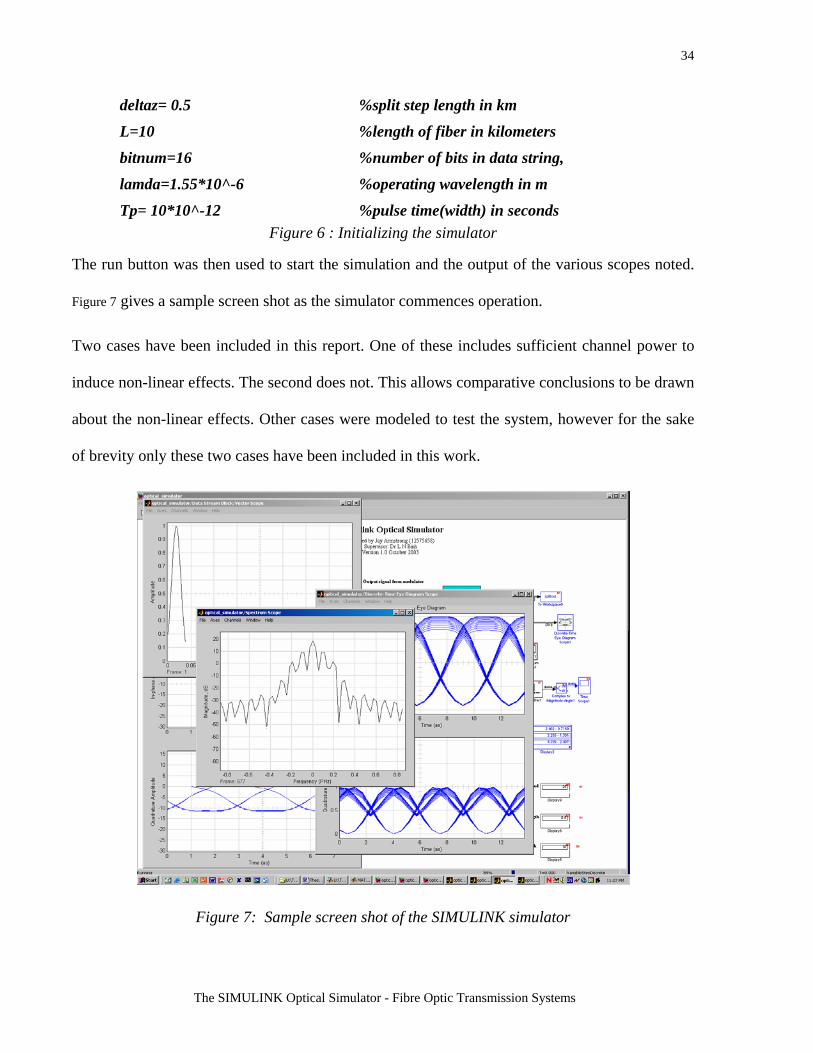
deltaz= 0.5 %split step length in km
L=10 %length of fiber in kilometers
bitnum=16 %number of bits in data string,
lamda=1.55*10^-6 %operating wavelength in m
Tp= 10*10^-12 %pulse time(width) in seconds Figure 6 : Initializing the simulator
The run button was then used to start the simulation and the output of the various scopes noted.
Figure 7 gives a sample screen shot as the simulator commences operation.
Two cases have been included in this report. One of these includes sufficient channel power to
induce non-linear effects. The second does not. This allows comparative conclusions to be drawn
about the non-linear effects. Other cases were modeled to test the system, however for the sake
of brevity only these two cases have been included in this work.
Figure 7: Sample screen shot of the SIMULINK simulator
MECSE-31-2004: "A SIMULINK Model for Simulation of Optical Communication ...", LN Binh and Jay Armstrong

35
The SIMULINK Optical Simulator - Fibre Optic Transmission Systems
To include non-linear effects a power input of 50mW was injected as the peak laser power input.
This value was above the threshold condition, 28.2mW, and resulted in an N parameter of (add N
value here). Such a system could be representative of a multiple channel optical transmission
system in which power levels as high as 100mW can be employed. For the low power
simulation a 5mW channel power was used. This would result in negligible non-linear effects
resulting in an N value of 1. This could represent a single channel or low channel count system.
The attained plots for these cases are shown in Figure 8.
The plots illustrate a number of key factors that occur when propagating an optical signal. In
particular the eye diagram can be used to determine the bit error rate. The spectrum scope plots
clearly illustrate the power of the carrier and its associated data sidebands. For comparative
purposes the same data stream was used in both the high and low power cases in order to
examine the non-linear effects on pulse distortion.
The advantage of the simulator is undoubtedly its versatility. One need not plot all this data
every time the simulation is run. Rather one can select the data most of use, such as the eye
diagram. This adds to the systems versatility by ensuring that only data relevant to the user is
displayed.
MECSE-31-2004: "A SIMULINK Model for Simulation of Optical Communication ...", LN Binh and Jay Armstrong

36
The SIMULINK Optical Simulator - Fibre Optic Transmission Systems
Figure 8(a) Gaussian-shape pulse train
MECSE-31-2004: "A SIMULINK Model for Simulation of Optical Communication ...", LN Binh and Jay Armstrong

37
The SIMULINK Optical Simulator - Fibre Optic Transmission Systems
Figure 8(b) Modulator output spectrum
Figure 8(c) Eye diagram at modulator output
MECSE-31-2004: "A SIMULINK Model for Simulation of Optical Communication ...", LN Binh and Jay Armstrong

38
The SIMULINK Optical Simulator - Fibre Optic Transmission Systems
Figure 8(d) Propagated output spectrum
MECSE-31-2004: "A SIMULINK Model for Simulation of Optical Communication ...", LN Binh and Jay Armstrong

39
The SIMULINK Optical Simulator - Fibre Optic Transmission Systems
Figure 8(e) Propagating output eye diagram
Figure 8: (a)-(e) 5mW simulation – Non-linear effects negligible, N=1
Figure 9(a) Shaped Gaussian pulse
Figure 9(b) Modulator output spectrum
MECSE-31-2004: "A SIMULINK Model for Simulation of Optical Communication ...", LN Binh and Jay Armstrong

40
The SIMULINK Optical Simulator - Fibre Optic Transmission Systems
Figure 9(c) Modulator output eye diagram
Figure 9(d) Propagated output spectrum
MECSE-31-2004: "A SIMULINK Model for Simulation of Optical Communication ...", LN Binh and Jay Armstrong

41
The SIMULINK Optical Simulator - Fibre Optic Transmission Systems
Figure 9(e) Propagated output eye diagram
Figure 9: 50mW case – Non-linear effects, N=0.429
A number of considerations can be drawn from the two case studies. Most importantly, the
effects of propagating an optical signal along a single step of fiber are clearly illustrated. A
comparison of the modulator output and the fiber output clearly shows the simulated dispersion
effects caused by the fiber. Figure 10 shows the modulator and fiber output plots attained for the
5mW laser/channel simulation.
The left hand side of Figure 10 shows the undistorted modulated eye diagram attained at the
output of the modulator. However, after propagation through the fiber, shown by the right hand
eye-diagram, the pulse is clearly broadened in accordance with the effects of GVD and PMD.
The clean eye opening demonstrated at the modulator output has lost some of its shape after
propagation through the fiber length. At the high power results, the pulse distortions due to the
MECSE-31-2004: "A SIMULINK Model for Simulation of Optical Communication ...", LN Binh and Jay Armstrong

42
The SIMULINK Optical Simulator - Fibre Optic Transmission Systems
non-linear effects are clearly shown. The GVD and PMD are still clearly evident. The pulses
have not only broadened but the eyes have also been partially closed. This would reduce a
systems margin for error and likely increase a systems bit error rate once a receiver was
incorporated.
Figure 10: Comparison of modulator output and fiber outputs for an input power of 5mW
5 CONCLUDING REMARKS Primarily a simulink optical transmission system and its various photonic components has been
established. Initial research focused upon the various technologies used such system. The
operation of these technologies has been deeply explored and in some cases developed for
MECSE-31-2004: "A SIMULINK Model for Simulation of Optical Communication ...", LN Binh and Jay Armstrong

43
The SIMULINK Optical Simulator - Fibre Optic Transmission Systems
further use. Negative dispersion usually occurs as a result of signal propagation through a
modulator, optical fiber or as a result of the optical carrier. Deliberately inducing a positive chirp
via the external modulator model, either through the tuning of the optical carrier or a phase shift
in the modulator may allow the limitations of chirp to be overcome.
To this end a fiber optic communication system simulation platform is developed. Based in the
Matlab subsidiary program, Simulink, this program can simplify the simulation process of
modern optical transmission systems. Simulink can simulate the fiber propagation through the
use of the split step method without difficulties. The dispersion effects of GVD, PMD and non-
linear factors were modeled independently over a short length of fiber. This allowed the
individual contribution of each effect to be analyzed. Also simulated were the operations of the
Mach-Zehnder Interferometric Modulator (MZIM) and its necessary components, the carrier and
the data stream. More importantly, the developed simulator provides a platform upon which a
powerful simulation tool can be developed.
Future works will aim to incorporate a greater number of optical components into the simulator,
further enhancing the uses of the simulator. The modeling of each effect over a short fiber length
can then be looped and iteratively calculated to model the performance of long haul optical
transmission systems. It is hoped that the optical simulator will provide the base framework upon
which optical transmission systems up to three thousand kilometers can be simulated.
This paper has outlined the flexibility of simulation techniques. Simulink provides a simple
means to upgrade the existing model. Another designer need not sift through pages of code and
variables in an attempt to understand the systems operation. Furthermore, a desire to incorporate
additional components, such as amplifiers, is relatively easily performed. A designed subset
modeling any given effect is simply placed within the propagation path. That means simulations
can be developed for numerous optical components and included or excluded at the user’s
MECSE-31-2004: "A SIMULINK Model for Simulation of Optical Communication ...", LN Binh and Jay Armstrong
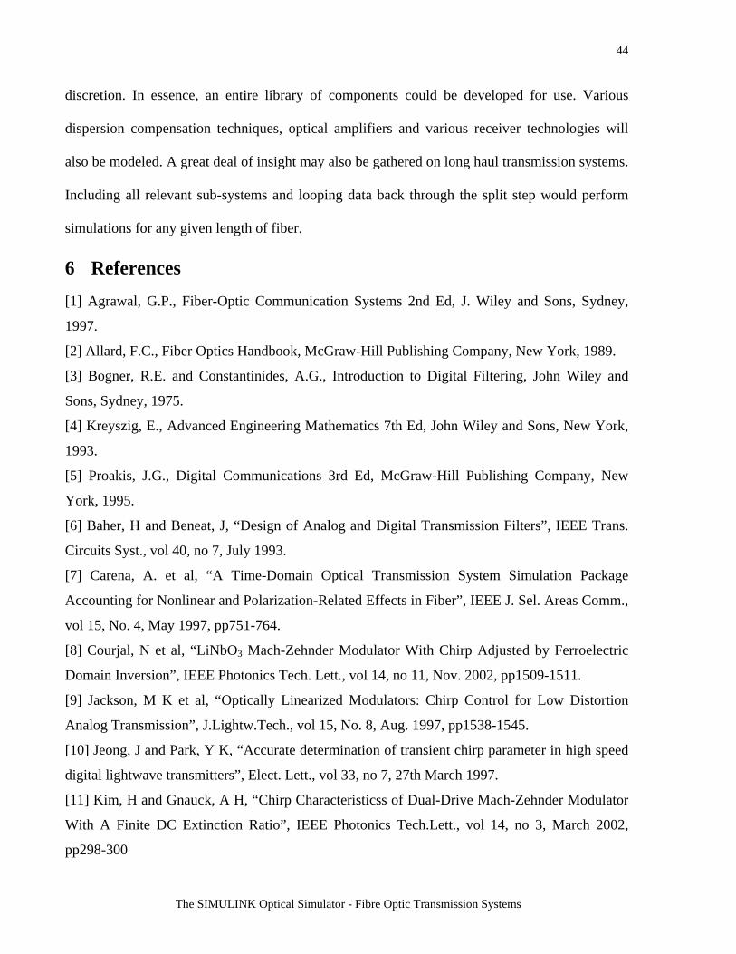
44
The SIMULINK Optical Simulator - Fibre Optic Transmission Systems
discretion. In essence, an entire library of components could be developed for use. Various
dispersion compensation techniques, optical amplifiers and various receiver technologies will
also be modeled. A great deal of insight may also be gathered on long haul transmission systems.
Including all relevant sub-systems and looping data back through the split step would perform
simulations for any given length of fiber.
6 References [1] Agrawal, G.P., Fiber-Optic Communication Systems 2nd Ed, J. Wiley and Sons, Sydney,
1997.
[2] Allard, F.C., Fiber Optics Handbook, McGraw-Hill Publishing Company, New York, 1989.
[3] Bogner, R.E. and Constantinides, A.G., Introduction to Digital Filtering, John Wiley and
Sons, Sydney, 1975.
[4] Kreyszig, E., Advanced Engineering Mathematics 7th Ed, John Wiley and Sons, New York,
1993.
[5] Proakis, J.G., Digital Communications 3rd Ed, McGraw-Hill Publishing Company, New
York, 1995.
[6] Baher, H and Beneat, J, “Design of Analog and Digital Transmission Filters”, IEEE Trans.
Circuits Syst., vol 40, no 7, July 1993.
[7] Carena, A. et al, “A Time-Domain Optical Transmission System Simulation Package
Accounting for Nonlinear and Polarization-Related Effects in Fiber”, IEEE J. Sel. Areas Comm.,
vol 15, No. 4, May 1997, pp751-764.
[8] Courjal, N et al, “LiNbO3 Mach-Zehnder Modulator With Chirp Adjusted by Ferroelectric
Domain Inversion”, IEEE Photonics Tech. Lett., vol 14, no 11, Nov. 2002, pp1509-1511.
[9] Jackson, M K et al, “Optically Linearized Modulators: Chirp Control for Low Distortion
Analog Transmission”, J.Lightw.Tech., vol 15, No. 8, Aug. 1997, pp1538-1545.
[10] Jeong, J and Park, Y K, “Accurate determination of transient chirp parameter in high speed
digital lightwave transmitters”, Elect. Lett., vol 33, no 7, 27th March 1997.
[11] Kim, H and Gnauck, A H, “Chirp Characteristicss of Dual-Drive Mach-Zehnder Modulator
With A Finite DC Extinction Ratio”, IEEE Photonics Tech.Lett., vol 14, no 3, March 2002,
pp298-300
MECSE-31-2004: "A SIMULINK Model for Simulation of Optical Communication ...", LN Binh and Jay Armstrong

45
The SIMULINK Optical Simulator - Fibre Optic Transmission Systems
[12] Koyama, F., “Frequency Chirping in External Modulators”, J. Lightw. Tech., vol 6, No. 1,
Jan. 1998, pp87-93.
[13] Laverdiere, C. et al, “A new method for measuring time-resolved frequency chirp of high bit
rate sources”, IEEE Photonics Tech. Lett., vol 15, no 3, March 2003, pp446-448.
[14] Saunders, R A et al, “Wideband chirp measurement technique for high bit rate sources”,
Elect. Lett., vol 30, no.16, Aug. 1994, pp1336-1338.
[15] Xie Y at al., “System Performance Degradation due to Nonlinear Signal Distortion in
Spectral Inverter”, J. Optical Comm., vol 19, no 4, 1998
[16] Binh, L.N., ECE4405: Optical Communication Systems Notes, Monash University, 2002
[17] Selliah, A., “Simulation of Polarisation Mode Dispersion Effects in A DWDM System: a
time domain approach”, Monash University Thesis, 2001.
7 APPENDIX %%%%%%%%%%%%%%%%%%%%%%%%%%%%%%%%%%%%%%%%%%%%%%%%%%%%%%%% % Simulink Optical Simulator initialisation % %%%%%%%%%%%%%%%%%%%%%%%%%%%%%%%%%%%%%%%%%%%%%%%%%%%%%%%% %before running simulator define the standard system parameters %then go to debug menu and select run, simulink model will automatically %open, press the run button in simulink to begin the simulation %standard system parameters bitrate=25*10^9 %bitrate in gb/s P0=50 %laser pulse power in mW (0.1 to 10 mW) deltaz=0.5 %split step length in km L=10 %length of fiber in kilometers bitnum=16 %number of bits in data string, lamda=1.55*10^-6 %operating wavelength in m Tp= 10*10^-12 %pulse time(width) in seconds %optional parameters varied for different fiber parameters r0=4.1*10^-6 %fiber spot size in m^2 n2=10^-20 %non-linear index coefficient in m^2/W D=17 %dispersion parameter in ps/nm.km speedlight=3*10^8 %speed of light in m/s %%%%%%%%%%%%%%%%%%%%%%%%%%%%%%%%%%%%%%%%%%%%%%%%%%%%%%%%%%%%%%%%%%%%%% %system functions, no need to vary these values %%%%%%%%%%%%%%%%%%%%%%%%%%%%%%%%%%%%%%%%%%%%%%%%%%%%%%%%%%%%%%%%%%%%%% time=(bitnum-1)*(1/bitrate) %simulation time for desired bit string I0=(P0+3.31)/0.133 %carrier current/amplitude iterations=L/deltaz
MECSE-31-2004: "A SIMULINK Model for Simulation of Optical Communication ...", LN Binh and Jay Armstrong

46
The SIMULINK Optical Simulator - Fibre Optic Transmission Systems
%defining carrier and pulse waveforms tc=0:5.155*10^-17:5.10345*10^-15 %define one period of carrier tc=tc' %convert tc to vertical matrix fc=1.94*10^14 %define the frequency of the carrier in Hz c=I0*sin(2*pi*fc*tc) %define carrier sinusoid carrier=[tc c] m=sin(2*pi*fc*tc+pi) %modulating waveform tg=-5*10^-9:0.55*10^-9:5*10^-9 %define gaussian pulse period t0=3.5*10^-9 %define standard deviation of gaussian pulse y=exp(-((tg/t0).^2)) % define gaussian pulse waveform gauss=[y] %need to determine whether non linear effects required Aeff=pi*(r0)^2 %calculatefiber effective area beta2=-((D*10^-6)*(lamda^2))/(-2*pi*speedlight)%calculate dispersion coefficient gamma=(2*pi*n2)/(lamda*Aeff) %calculate nonlinear coefficient Ld=(Tp^2)/(abs(beta2)) %calculate the dispersion length Preq=(abs(beta2))/(gamma*(Tp^2)) %power required to generate pulse in Watts P0=P0*10^-3 if P0<(Preq/10) %check non linearity limit and determine non linear parameter N=1 %if fiber power < pulse required per pulse non-linearities negligable else N=(gamma*Ld*P0)^0.5 %If fiber power >= pulse required incorporate non linear effects end open('E: \Optical Simulator\optical_simulator.mdl') %open simulator model in simulink, may need to alter path if not on %installation disk %%%%%%%%%%%%%%%end initialisation file%%%%%%%%%%%%%%%%%%%%%%%%
MECSE-31-2004: "A SIMULINK Model for Simulation of Optical Communication ...", LN Binh and Jay Armstrong