A SIMPLIFIED MODEL FOR SOCIAL WELFARE ANALYSIS

Review of Income and Wealth Series 44, Number 1, March 1998

A SIMPLIFIED MODEL FOR SOCIAL WELFARE ANALYSIS:

AN APPLICATION TO SPAIN, 1973-74 TO 1980-81

Universidad Carlos III de Madrid

Most of the literature on income distribution has concentrated on inequality. In this paper we introduce a concern for efficiency in a social welfare model. We propose a simple but useful specification which combines three features: (i) the selection of measurement instruments in the relative and the absolute case on the grounds of their properties for applied work; (ii) a procedure to make welfare comparisons across households with different needs, in a model in which equivalence scales depend only on household size; and (iii) the use of household specific statistical price indices to make intertemporal comparisons in real terms. The methodology is applied to the study of the role of prices and demographic effects in the evolution of the standard of living in Spain from 1973-74 to 1980-81.

Most of the analytical and empirical literature on income distribution has concentrated on income inequality. In this paper we propose a simplified but convenient social welfare model which reflects also a concern for efficiency. The model is then applied to the evolution of the standard of living in Spain using two household budget surveys for 1973-74 and 1980-81. The main features of the approach are the following four.

(i) As Dutta and Esteban (1991) have shown, to express social or aggregate welfare in terms of only two statistics of the income distribution-the mean, and a measure of inequality-we need to specify the type of mean-invariance property we want our inequality indices to satisfy. This is politically important, since we know from the early discussion in Kolm (1976) that the choice of a mean-invariance class of inequality measures is not merely a technical matter, but a value laden question.' In this paper, we consider two polar cases: the usual relative inequality concept, according to which a proportional change in all incomes leaves the level of inequality unchanged; and an absolute inequality concept, very seldom applied in empirical analysis, according to which inequality remains constant only if all individuals experience the same absolute income change.

(ii) We are interested in complete indicators which permit the decomposition of welfare changes into changes in the mean, and changes in either relative or absolute inequality. Which of these social evaluation functions (SEFs for short)

Note: This work is part of a larger project carried on under the auspices of the chair Gumersindo de Azarate, presently occupied by the author and funded by the Ministerio de Trabajo y Asuntos Sociales of Spain. The excellent research assistance provided by Miguel Angel Benito and Mercedes Sastre, whose work has been partly financed by Project PB93-0230 of the Spanish DGICYT, is gratefully acknowledged. Two anonymous referees and the editor helped to improve considerably the original version. Only the author is responsible for all remaining shortcomings.

' ~ e c e n t reports based on questionnaires indicate that people are by no means unanimous in their choice between relative, absolute or other intermediate notions of inequality. See, for instance, Amiel and Cowell (1992), and Ballano and Ruiz-Castillo (1994).

should we use in applied work? It turns out that the conditions usually required for an admissible SEF plus an interesting decomposability property, lead to specific functional forms: in the relative case, to a single member of the generalized entropy family and, in the absolute case, to the Kolm-Pollak family indexed by a parameter representing degrees of aversion to inequality.

(iii) We assume that the only characteristic which gives rise to different needs for social evaluation purposes is household size. The problem, of course, is that to pool all households into a unique distribution we need a procedure to compare non-income needs across household sizes. In the relative case, following Buhman et al. (1988) and Coulter et al. (1992a, b), we use a parametric model of equivalence scales which allows for different views about the importance of economies of scale in consumption within the household. We extend the model to the absolute case and establish the connection between the parametrization of economies of scale in both cases.

(iv) To introduce the distributional role of changes in relative prices in intertemporal comparisons we use household specific statistical price indices. Since statistical price indices provide only convenient bounds to the true cost-of-living constructions, we show how our estimates also provide equally convenient bounds to the change in the mean and inequality in real terms. We illustrate the advantages of our procedure by comparing our results with those obtained by adopting the usual assumption of a single inflation rate common to all households.

These measurement tools and methodological conventions are applied to Spanish data from two large household budget samples, of about 24,000 observations each : the Encuestas de Presupuestos Familiares (EPF for short), collected in 1973-74 and 1980-81 by the Spanish Znstituto Nacional de Estadistica with the main purpose of estimating the base weights of the official system of Consumer Price Indices. Like Slesnick (1991, 1993), we propose to identify a household standard of living with current commodity consumption. We argue that, in our case, this is better approximated by a measure of current total household expenditures, net of expenditures on the acquisition of certain durables.

During this period, right after the first oil crisis and in the middle of a radical political change in Spain, according to National Accounts data GNP grew at an average annual rate of about 2.3 percent at constant prices of 1986, while according to the Consumer Price Index there was a 322 percent inflation rate. In this context, our main empirical conclusions are the following:

(i) Our estimates provide very good bounds for the real change in the mean and relative inequality. Therefore, we can safely conclude that welfare for the population as a whole has improved between 10-1 1 percent in the relative case.

(ii) When we apply the same inflation rate to all households in 1973-74, estimates of welfare change are similar to those obtained with household specific price indices. However, in this case we only capture the inequality change in money terms. Given that relative prices in Spain have evolved during this period in a pro-poor direction, the true improvement of inequality in real terms becomes understated. As a consequence, too much of the real welfare improvement is wrongly attributed to an increase in the mean.

(iii) During this period, dominated by the first oil crisis and other adverse economic circumstances in Spain, there is a moderate increase in mean household

124

expenditures in real terms of about 4-7 percent. As we reported in Ruiz-Castillo (1995a), real inequality decreased between 15-20 percent according to the relative inequality index we use in this paper. One way to appreciate the magnitude of such change, is provided by the following unusual finding: absolute inequality for the total population decreased for all values of the equivalence scale parameter. We estimate a welfare increase in the absolute case which ranges from 38,000 to 55,000 pesetas, or from 27,000 to 48,000 pesetas, depending on the value of the aversion to inequality parameter.

(iv) There are considerable variations among subgroups in the partition by household size. In particular, there are exceptions to the generalized improvement in inequality: as the parameter reflecting the aversion to inequality increases there are two household sizes for which absolute inequality increases. By the use of decomposable measurement instruments we are able to understand how results at the household level get translated to the population as a whole. In both the relative and the absolute case most of our results are rather robust to changes in the parameters which reflect the generosity of the equivalence scales.

The rest of the paper is organized in four sections and a brief statistical Appendix. The first section presents the measurement framework, which includes the parametrization of equivalence scales in the relative and the absolute case, the social evaluation functions, and the nature of our approximation to social welfare change using statistical price indices. The second section is devoted to the measurement of a household standard of living. The third section contains the empirical results, while the final section offers some concluding remarks on the potential implications of our results for similar studies in other countries.

1.1. Interhousehold Welfare Comparisons

Suppose we have a population of h = 1, . . . , H households which can differ in a single dimensional variable-say, income-representing its standard of living, xh, and/or a vector of household characteristics. In this paper, households of the same size are assumed to have the same needs and, therefore, their incomes are directly comparable. Consequently, we believe that it is important to investigate separately each of the subgroups in the basic partition by household size. However, social evaluation within subgroups need not yield unanimous results. Moreover, it is always convenient to extract conclusions for the population as a whole. Therefore, we need a procedure to establish inter-household welfare comparisons. This is, of course, the role played by equivalence scales.

We assume that larger households have greater needs, but also greater oppor- tunities to achieve economies of scale in consumption. Denote household size by sh and, for each household h, define adjusted income in the relative case by

Assume there are m = 1, . . . ,M household sizes. If we think of a single adult as the reference household, the expression 1/me can be interpreted as the number of equivalent adults in a household of size m. Thus, the greater is 0, the greater

125

the number of equivalent adults for each household or, in other words, the smaller the economies of scale. When 0 = 0 and economies of scale are assumed to be infinite, adjusted income coincides with unadjusted household income; while if 0= 1 and economies of scale are completely ruled out, then adjusted income equals per capita household income.

In the absolute case, for each household h of size m, define adjusted income by

yh ( A m ) = xh - Am(m - 1 ) .

The parameter Am can be interpreted as the cost of a reference adult when household size is m. Thus, for each m economies of scale vary inversely with Am.

Let xm be the vector of original incomes for households of size m. Notice that, if I ( . ) is any scale invariant index of relative inequality, then we have

Similarly, if A ( . ) is any translation invariant index of absolute inequality, then we have

Thus, the two models share the convenient property that, within each ethically homogeneous subgroup, the adjustment process does not alter the underlying inequality: the inequality of adjusted income is equal to the inequality of original income.

The only remaining question is the following. The unit interval provides a natural range of variation for the parameter O in the relative case, but how do we fix Am for each m in the absolute case? The following procedure permits us to establish a connection between the parametrization of equivalence scales in the two cases. Let y m ( 0 ) and ym(Am) be the adjusted income vectors for households of size m in the relative and the absolute case, respectively, and let p ( . ) denote the mean of any distribution. Given O , we choose Am(@) for each m so that the mean of both vectors is the same, that is, so that

It is easy to see that this condition implies:

( 1 ) Am(@) = [ p ( y m ( 0 ) ) ( m @ - l ) ] / ( m - 1) = [ p ( x m ) ( m @ - l ) ] / [ ( m - l )m@] .

Thus, the greater O is, the greatest is Am and the smaller are the economies of scale.

1.2. Admissible Social Evaluation Functions

A SEF is a real valued function W defined in the space R~ of adjusted incomes, with the interpretation that for each income distribution y= ( y ' , . . . , y H ) , W ( y ) provides the "social" or, simply, the aggregate welfare from a normative point of view. Let us assume that our SEFs satisfy the requirements discovered by Dutta and Esteban (1991) for expressing welfare as a function of the mean and an index of relative or absolute inequality. In addition, let us adopt

a multiplicative or an absolute trade off between the mean and inequality in the relative and the absolute case, respectively. However, which SEFs within these classes should we use in applied work? The following property leads us to an appropriate selection.

Suppose that we have two islands where income is equally distributed but whose means are different. If they now form a single entity, there will be no within-island inequality but there would be inequality between them. In income inequality theory we search for additively separable measures capable of expressing this intuition. In our context, for any partition we are interested in expressing social welfare for the population as the sum of two terms: a weighted average of welfare within the subgroups, with weights equal to demographic shares, minus a term which penalizes the inequality between subgroups. In this case, we say that the SEF is additively decomposable.

Let y* be the distribution in which each household is assigned the mean income of the subgroup to which it belongs in the partition by household size, p(xm). Let I , ( . ) be the first index of relative inequality originally suggested by Theil :

Consider SEFs which can be expressed as the product of the mean and a term equal to one minus a relative inequality index of the Generalized Entropy class. Ruiz-Castillo (1995b) shows that the only SEF among them with the property of additive decomposability with demographic weights, is the following:

where Hm is the number of households of size m, so that C,Hm = H. Thus, social welfare is seen to be a weighted average of the welfare within each subgroup with weights equal to demographic shares, minus the between-group inequality weighted by the population mean.

In the absolute case, Blackorby et at. (1981) show that analogous requirements lead to the Kolm-Pollak family of SEFs:

where y is interpreted as an aversion to inequality parameter: as y increases, social indifference curves show increasing curvature until, in the limit, only the poorest household income matters. The absolute inequality index associated with W, is

Let us denote by t* the distribution in which each household is assigned the equally distributed equivalent income of the subgroup to which it belongs, t (xm). Then

so that

Thus, social welfare is equal to the mean minus the Kolm-Pollak absolute inequality index. On the other hand, social welfare is a weighted average of the welfare within each subgroup with weights equal to demographic shares, minus the inequality between the subgroups.2

Taking into account our definitions of adjusted income, in the relative case we have

where p*(@) is the distribution in which each household is assigned the mean income of the subgroup to which it belongs in the partition by household size, p(y"(@)). In the absolute case, let A(@) = (A I ( @ ) , . . . , AM(@)) be the vector of equivalence scale parameters fixed as in equation (1). Then we have

where <*(A(@)) is the distribution in which each household is assigned the equally distributed equivalent income of the subgroup to which it belongs, 5 (f(0)).

In welfare economics we are mostly interested in personal welfare, rather than in household welfare. Following standard practice, we can extend the SEF domain to distributions in which each household adjusted income is weighted by household size or, in other words, in which each person is assigned the adjusted income of the household to which she belongs. The above formulas for W and KP, can be easily transformed for this case: demographic shares, Hm/H, as well as expressions p*(@) and <*(A(@)), must be replaced by their counterparts in the distribution of persons.

1.3. The Nature of Our Approximation in the Presence of the Substitution Bias of Statistical Price Indices

Omitting here any reference to the parameter @ to simplify the notation, let y l=(y; , . . . , y r ) and y2=(y;, . . . , yr ' ) be the vector of adjusted household expenditures in the two situations under comparison. Suppose we want to compare yl and y2 in real terms at prices of situation 2, p2. Let yi2 be household h's adjusted income in situation 1 expressed at prices p2. Ideally we would compute yf2 = yf L(p2, P I ; uf ), where L(p2, P I ; u:) is a true cost-of-living index of the Las- peyres type and d is the utility level achieved by household h in situation 1. Similarly, to compare yl and y2 in real terms at prices of situation 1, p l , we would use for each household the expression y';l zy'; /p(p2, p, ; u'; ), where P(p2, P I ; u'; ) is a true cost-of-living index of the Paasche type and u'; is the utility level achieved by household h in situation 2.

In this favourable case, how would the classical number index problem mani- fest itself? To answer this question, we must review the formulas for social welfare change we use in the sequel. Recall that in the relative case, for example, social

20f course, both in the relative and the absolute case the property of decomposability is essential for the study of any other partition. For an application to partitions by geographic and socioeconomic characteristics, which will not be treated here, see Ruiz-Castillo (1995~).

welfare at any period z = 1,2 is equal to

w(Yr)=~(Y,)[l-Il (Yr)l.

To evaluate the social welfare change at constant prices p2, we compare the distributions y2 and y12 by means of the expression

where

and

(4)

Equation (2) measures the real change in the mean. Equation (3) reflects the change in real inequality. It is greater (smaller) than one as real inequality decreases (increases) in period 2 relative to period 1. Equation (4) measures the change in real welfare. Let us denote by A W(pl ), Ap(pl ), and AE(p1) the corresponding expressions for the social evaluation problem at pricespl, which involves the comparison of distributions yz1 and yl . Notice that there are no a priori reasons for Ap2 (p2) or AE(p2) to be greater or smaller than Ap(pl ) or AE(pl), respectively. Hence, nothing can be said on theoretical grounds about the relationship between A W(p2) and A W(p,). Nevertheless, in an empirical situation one hopes that these two magnitudes are close to each other.

To carry on the above program, we need to estimate a complete demand system in order to compute the true cost-of-living indices. In this paper, we propose to approximate the index L(p2,pl ; u:) for each h by its upper bound L(p2, p l ; w:), where w: is the vector of total expenditure commodity shares of household h in situation 1. Similarly, we propose to approximate the index P(p2,pl ; u$) by its lower bound P(p2,pl; w:), where w$ is the vector of total expenditure commodity shares of household h in situation 2. Let us denote our estimates of yt2 and y:, by zf2 = y'; L(p2 , pl ; w: ) and z& = yh2 / P ( ~ ~ , p l ; w: ), respectively. The question is: which is the nature of our approximations to the true changes in the mean, inequality and welfare in real terms?

It should be clear that, because of the substitution bias of our household specific price indices, for each h our constructions zt2 and zil overestimate the true ones, yf2 and y$,, respectively. Two important consequences follow from here. In the first place, taking into account equation (2), our estimates for the real change in the mean at prices p2 [pl ] provide a lower (upper) bound for their true value, Ap(p2) [Ap(pl)]. In the second place, let us adopt the reasonable assumption that the substitution bias is greater for the rich than the poor. Assume also that the change in relative prices from p l to p2 is less damaging to the poor than to the rich, as we know to be the case for Spain in this period. Then, following the argument given in Ruiz-Castillo (1995b), it can be shown that our estimates at p2 [pI ] for the expressions AE(p2) [AE(pl )] provide an upper (lower) bound for the true constructions.

129

Therefore, nothing definite can be said about the relationship between our estimates and the true values for A W(p2) and A W(pl ). However, in any empirical situation one would like to obtain that Ap(p2) <Ap(pl ) and AE(p2) 2 AE(pl ), in the hope that the true changes in the mean and in relative inequality lie between these limits. In this case, our estimates for A W(p2) and A W(pl) have a good chance of being close to each other.3

Our data comes from two large budget surveys collected in 1973-74 and 1980-8 1. They consist of 24,15 1 and 23,707 observations, representative of a population of approximately 9 and 10 million households, respectively, occupying residential housing in all of Spain except the northern African cities of Ceuta and Melilla.

The EPFs are spread out uniformly over a period of 52 weeks. All household members of 14 or more years of age are supposed to record all expenditures which take place during a sample week. Then, in depth interviews are conducted to register past expenditures over reference periods beyond a week and up to a year. From that information, the INE estimates annual household total e ~ ~ e n d i t u r e s . ~ On the other hand, a maximum of four income recipients are asked about the income earned from different sources during the year prior to the sample week. Therefore, household expenditures and household income are not estimated for the same period.

Given the nature of our data, we have several reasons for choosing household expenditures rather than household income to approximate a household standard of living. (i) There is a general presumption that current expenditure is a better proxy of permanent income than current income which includes more volatile transitory components. (ii) Although the EPF's include valuable information on income perceived by a maximum of four household members, the surveys are primarily designed to measure household expenditure with the purpose of estimating the Consumer Price Index weighting system. Therefore, we expect the INE to devote more care and attention to the expenditure side. (iii) Several individuals might be inclined to underreport income. For instance, those working in the underground economy, the self-employed, professionals of all sorts, or people working in the agricultural sector. However, none of them are particularly prone to missreport their expenditures. Therefore, we expect that expenditures for those individuals are better measured than income. On the other hand, we expect respon- dents to report equally well their expenditures on goods and services acquired in either the underground or the regular economy. Therefore, the activities of both demanders and suppliers of the underground economy are better captured through the expenditure side. (iv) It turns out that INE's estimates of total expenditures for more than 60 percent of households are greater than household i n ~ o m e . ~

30f course, an entirely analogous problem must be faced in the absolute case. 4 ~ y taking into account the available information on bulk purchases, Peiia and Ruiz-Castillo

(1998) improved upon INE's original estimates of annual food and drinks expenditures. Our measure of household total expenditures includes the corresponding correction.

his is in agreement with results in Sanz (1996) showing a loss close to 23 percent when income information in the EPF's is compared with National Accounts data.

Moreover, contrary to all expectations, there is evidence showing less total income inequality than total expenditure inequality.6 In our opinion, these facts need some explanation before income data can be comfortably used.

In addition to the above reasons to prefer the EPF measure of household expenditures, we agree with Slesnick (1991, 1993) that, ideally, we should identify the standard of living with commodity consumption. Lacking information on leisure and public goods consumption, our starting point must be household total expenditures as an approximation to household consumption of private goods and services.

The EPF has a rather wide co&ept of total expenditure, including expenditures on items not covered by the Consumer Price Index (like funeral articles; contributions to non-profit institutions; gambling expenditures; fines; hunting, fishing and other fees), as well as a number of imputations for home production, wages in kind and subsidized meals at work. To avoid double counting, transfers to other households or to household members absent from home are excluded.

Our experience with the 1980-81 EPF indicates that discontinuous household expenditures on some durables, whose occurrence may distort heavily the total, are best considered investment rather than c o n ~ u m ~ t i o n . ~ These refer to current acquisitions of cars, motorcycles and other means of private transportation, as well as house repairs financed by either tenants or owner-occupiers. Life and housing insurance premiums are excluded on the same grounds. Thus, our estimate of household current consumption equals total household expenditures, net of these investmat items.

Ideally, we should include an estimate of the consumption services currently provided by these investment flows as well as by the stock of household durables acquired in the past. We do this for housing-without doubt the more important household durable-since the INE includes a market rental value for owner- occupied housing, as well as for the rest of the stock which is neither rented nor owned by the household occupying it. Such rental values are estimated by the owner or the occupying household, respectively.

111.1 Changes in Real Terms Within the Partition by Household Size

a. The Change in Mean Household Expenditures

We begin by investigating the role of prices in inequality and welfare comparisons within each subgroup in the partition by household size. Our data were collected from July 1973 to June 1974 (situation I), and from April 1980 to March 1981 (situation 2). Since we have information on the quarter in which each household was interviewed in the 1980-81 EPF, we choose p2=winter of 198 1. Since this is not the case for the 1973-74 EPF, we choose p, = (1 /2)p7, + (1/2)p74.8 In what follows, we denote by zl and z12 the 1973-74 expenditure

%ee Ayala et al. (1993) and Del Rio and Ruiz-Castillo (1996). 'see Ruiz-Castillo (1987). 'statistical price indices were constructed using a 58 commodity breakdown for which the INE

publishes monthly price data at the national level. For a detailed analysis of this topic, see Sastre (1998).

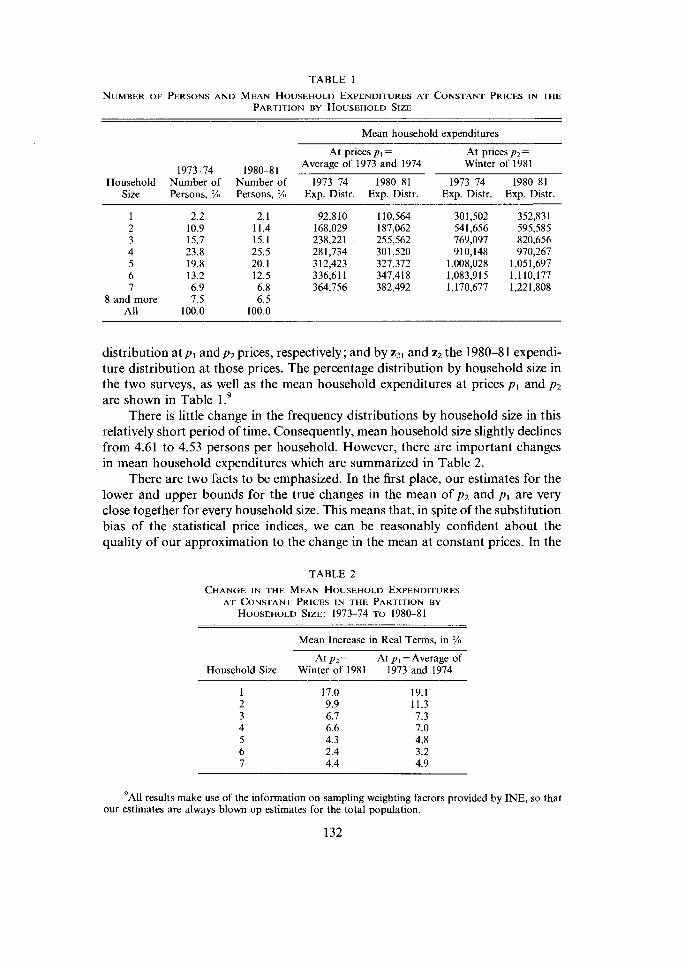
TABLE 1

NUMBER OF PERSONS AND MEAN HOUSEHOLD EXPENDITURES AT CONSTANT PRICES IN THE

PARTITION BY HOUSEHOLD SIZE

Mean household expenditures

At prices p, = At prices p, =

1973 74 1980-81 Average of 1973 and 1974 Winter of 198 1

Household Number of Number of 1973-74 1980-81 1973-74 1980-81 Size Persons, % Persons, % Exp. Distr. Exp. Distr. Exp. Distr. Exp. Distr.

1 2.2 2 10.9 3 15.7 4 23.8 5 19.8 6 13.2 7 6.9

8 and more 7.5 All 100.0

distribution at pl andp, prices, respectively; and by zzl and z2 the 1980-81 expenditure distribution at those prices. The percentage distribution by household size in the two surveys, as well as the mean household expenditures at prices p l and p2 are shown in Table 1.9

There is little change in the frequency distributions by household size in this relatively short period of time. Consequently, mean household size slightly declines from 4.61 to 4.53 persons per household. However, there are important changes in mean household expenditures which are summarized in Table 2.

There are two facts to be emphasized. In the first place, our estimates for the lower and upper bounds for the true changes in the mean of p2 and pl are very close together for every household size. This means that, in spite of the substitution bias of the statistical price indices, we can be reasonably confident about the quality of our approximation to the change in the mean at constant prices. In the

TABLE 2

Mean Increase in Real Terms, in %

At p2 = At p , =Average of Household Size Winter of 1981 1973 and 1974

9 ~ 1 1 results make use of the information on sampling weighting factors provided by INE, so that our estimates are always blown up estimates for the total population.

132

second place, although all households experience some increase in the mean, the improvement is inversely related to household size. Single person and two person households-representing about 28 percent of all households and 13 percent of all persons-have 18 and 10 percent increases. The important group of 3 and 4 person households-representing about 40 percent of both households and persons-have a 7 percent increase. Finally, large households of 5 to 7 persons- representing 26 percent of all households and 40 percent of all persons+xperience a small increase of 2-5 percent.

b. Welfare Change in the Relative Case

Social welfare is a function of efficiency and distributional considerations. In the relative case, for any period z our SEF expresses a multiplicative trade off between these two forces

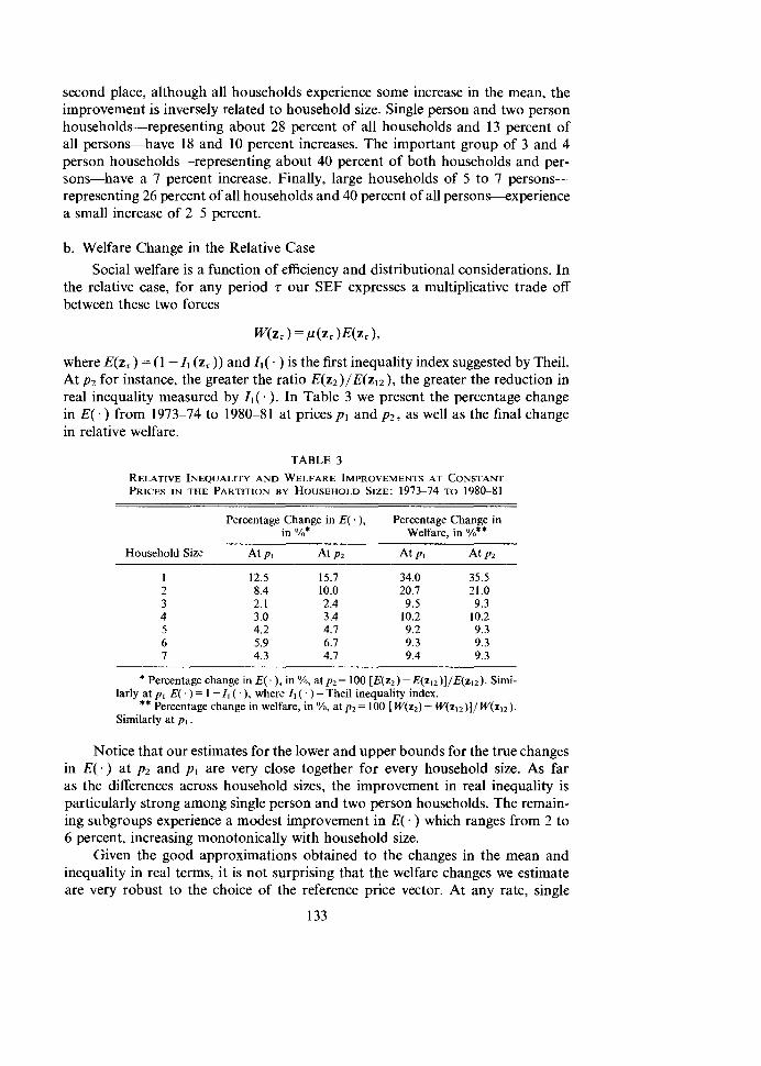
where E(z , ) = (1 - Zl ( 2 , ) ) and Z l ( . ) is the first inequality index suggested by Theil. At p2 for instance, the greater the ratio E(z2) /E(z12) , the greater the reduction in real inequality measured by I , ( . ) . In Table 3 we present the percentage change in E( . ) from 1973-74 to 1980-81 at prices pl and pz, as well as the final change in relative welfare.

TABLE 3

Percentage Change in E ( . ) , Percentage Change in in %* Welfare, in %**

Household Size At P I At p2 At P I At p2

* Percentage change in E ( . ) , in %, atp2= 100 [E(zz ) - E(zI2) ] /E(zI2) . Simi- larly at pl E( . ) = 1 - I l (. ), where I, ( . ) = Theil inequality index. ** Percentage change in welfare, in %, at p2= 100 [ W(z2) - W ( z I 2 ) ] / W(z I2 ) . Similarly at p, .

Notice that our estimates for the lower and upper bounds for the true changes in E( . ) at p2 and pl are very close together for every household size. As far as the differences across household sizes, the improvement in real inequality is particularly strong among single person and two person households. The remaining subgroups experience a modest improvement in E ( . ) which ranges from 2 to 6 percent, increasing monotonically with household size.

Given the good approximations obtained to the changes in the mean and inequality in real terms, it is not surprising that the welfare changes we estimate are very robust to the choice of the reference price vector. At any rate, single

person and two person households experience an increase of 35 and 21 percent in real relative welfare, respectively, while the remaining subgroups present only a 9- 10 percent increase.

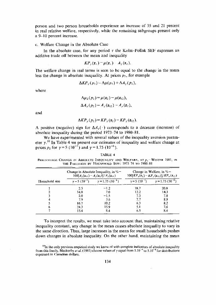
c. Welfare Change in the Absolute Case

In the absolute case, for any period z the Kolm-Pollak SEF expresses an additive trade off between the mean and inequality

KP,(zr)=P(zr)-A,(z,).

The welfare change in real terms is seen to be equal to the change in the mean less the change in absolute inequality. At prices p2, for example

AKP,(P2)=AP(P2)+- AA,(p2),

where

and

AKP, (PZ) =KPy (22) - KP, (212).

A positive (negative) sign for AA,(.) corresponds to a decrease (increase) of absolute inequality during the period 1973-74 to 1980-8 1.

We have experimented with several values of the inequality aversion parameter y.10 In Table 4 we present our estimates of inequality and welfare change at pricesp2 for y = 5 (lop7) and y = 1.75 ( IO-~) .

TABLE 4

PERCENTAGE CHANGE I N ABSOLUTE INEQUALITY AND WELFARE, AT p2= WINTER 1981, IN

THE PARTITION BY HOUSEHOLD SIZE: 1973-74 TO 1980-81

Change in Absolute Inequality, in %= Change in Welfare, in % =

100IAr(z,,) -A7(z2)1/Ar(z~2) 1OO[Kpr(z2)-KPr (zI~)I/KP, (~12)

Household size y = 5 (lo-') y = 1.75 y=5(10-') y=1.75(10-~)

1 2.5 -1.2 18.7 20.8 2 14.8 7.0 12.2 14.3 3 2.0 -1.5 7.3 7.8 4 7.9 3.6 7.7 8.9 5 16.7 10.2 6.3 8.2 6 24.3 15.9 5.1 7.6 7 15.4 8.4 6.5 8.4

To interpret the results, we must take into account that, maintaining relative inequality constant, any change in the mean causes absolute inequality to vary in the same direction. Thus, large increases in the mean for small households pushes down changes in absolute inequality. On the other hand, maintaining the mean

10 In the only previous empirical study we know of with complete indicators of absolute inequality from this family, Blackorby et al. (1981) choose values of y equal from 5.10-~ to 5.10-~ for distributions expressed in Canadian dollars.

constant, a change in relative inequality causes a change in the same direction in absolute inequality.

The main result is that, given the general improvement in relative inequality, most subgroups experiment an improvement in absolute inequality. Such an improvement appears to be greater for larger households whose mean increases are smaller (see Table 2). It should be noticed that, as the aversion to inequality increases, the percentage inequality change from 1973-74 to 1980-81 generally decreases, becoming negative for single person and three person households. The reason for this is that single person households experience large mean increases, while three person households have the smallest improvement in relative inequality (see Table 3).

In comparison to the relative case, percentage changes in absolute welfare are somewhat smaller for all household sizes. However, the pattern across subgroups is maintained: single person and two person households experience approximately a 19 or 13 percent improvement, while the remaining subgroups exhibit only a 5-7 or a 7-9 percent increase depending on the choice of the aversion to inequality parameter."

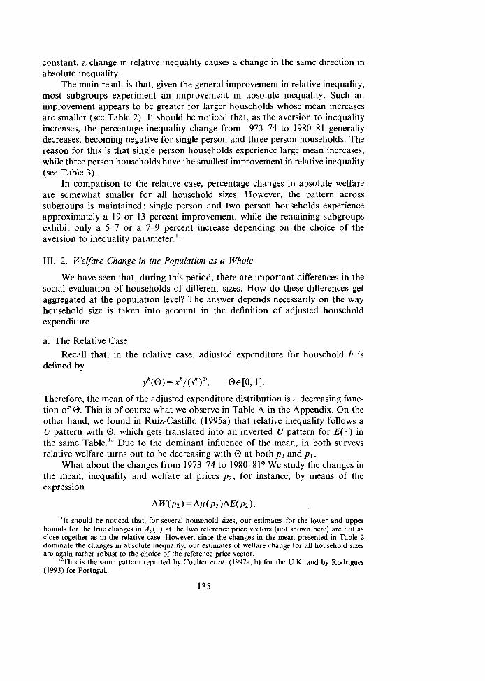
111. 2. Welfare Change in the Population as a Whole

We have seen that, during this period, there are important differences in the social evaluation of households of different sizes. How do these differences get aggregated at the population level? The answer depends necessarily on the way household size is taken into account in the definition of adjusted household expenditure.

a. The Relative Case

Recall that, in the relative case, adjusted expenditure for household h is defined by

yh(0) = xh/(sh)@, OE [0, 11.

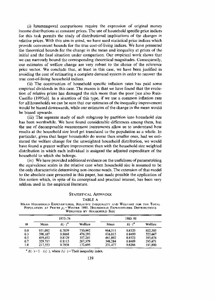
Therefore, the mean of the adjusted expenditure distribution is a decreasing function of O. This is of course what we observe in Table A in the Appendix. On the other hand, we found in Ruiz-Castillo (1995a) that relative inequality follows a U pattern with O, which gets translated into an inverted U pattern for E( . ) in the same ~ a b 1 e . I ~ Due to the dominant influence of the mean, in both surveys relative welfare turns out to be decreasing with O at both p2 and p, .

What about the changes from 1973-74 to 1980-81? We study the changes in the mean, inequality and welfare at prices p2, for instance, by means of the expression

"1t should be noticed that, for several household sizes, our estimates for the lower and upper bounds for the true changes in A , ( . ) at the two reference price vectors (not shown here) are not as close together as in the relative case. However, since the changes in the mean presented in Table 2 dominate the changes in absolute inequality, our estimates of welfare change for all household sizes are a ain rather robust to the choice of the reference price vector.

h h i s is the same pattern reported by Covlter rr ol. (199Za. b) for the U.K. and by Rodrigurn (1993) for Portugal.

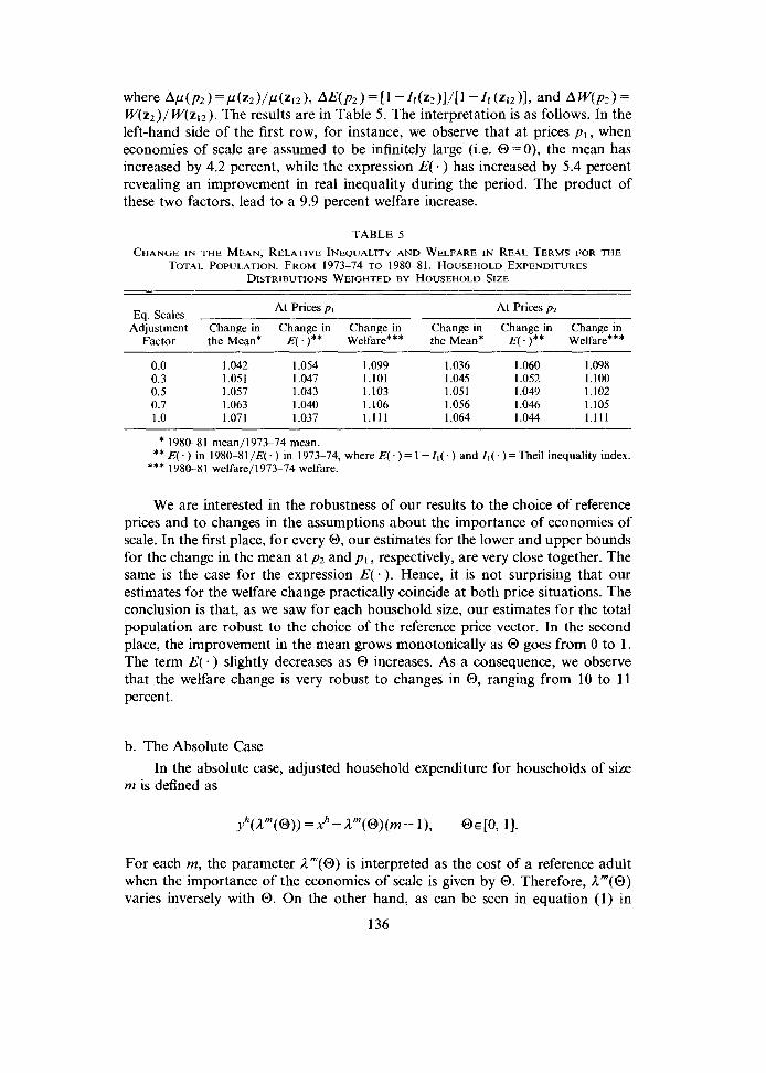
where A P ( P ~ ) = P ( Z ~ ) / P ( Z I ~ ) . AE(p2)=[1 -I1(~2)1/ [1 -Z1(z12)1, and AW(p2)= W(z2) / W ( z I 2 ) . The results are in Table 5. The interpretation is as follows. In the left-hand side of the first row, for instance, we observe that at prices p l , when economies of scale are assumed to be infinitely large (i.e. 0=0), the mean has increased by 4.2 percent, while the expression E ( . ) has increased by 5.4 percent revealing an improvement in real inequality during the period. The product of these two factors, lead to a 9.9 percent welfare increase.

TABLE 5

At Prices p l At Prices p, Eq. Scales

Adjustment Change in Change in Change in Change in Change in Change in Factor the Mean* E( . )** Welfare*** the Mean* E( . )** Welfare***

* 1980-81 mean/1973-74 mean. ** E(. ) in 1980-81/E(. ) in 1973-74, where E( . ) = 1 - I l ( . ) and I , ( . ) = Theil inequality index.

*** 1980-81 welfare/1973-74 welfare.

We are interested in the robustness of our results to the choice of reference prices and to changes in the assumptions about the importance of economies of scale. In the first place, for every 0, our estimates for the lower and upper bounds for the change in the mean at p2 and pl , respectively, are very close together. The same is the case for the expression E ( . ) . Hence, it is not surprising that our estimates for the welfare change practically coincide at both price situations. The conclusion is that, as we saw for each household size, our estimates for the total population are robust to the choice of the reference price vector. In the second place, the improvement in the mean grows monotonically as O goes from 0 to 1. The term E ( - ) slightly decreases as O increases. As a consequence, we observe that the welfare change is very robust to changes in 0, ranging from 10 to 1 1 percent.

b. The Absolute Case

In the absolute case, adjusted household expenditure for households of size m is defined as

For each m, the parameter A m ( @ ) is interpreted as the cost of a reference adult when the importance of the economies of scale is given by O. Therefore, A m ( @ ) varies inversely with O. On the other hand, as can be seen in equation ( I ) in

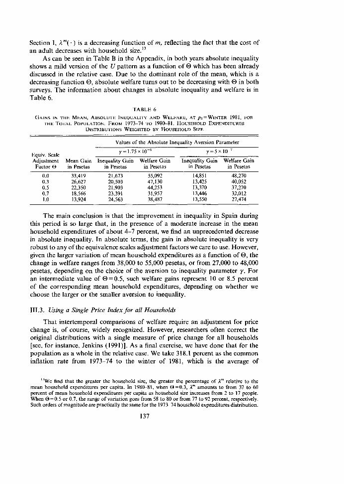
Section I, A m ( . ) is a decreasing function of m, reflecting the fact that the cost of an adult decreases with household size.13

As can be seen in Table B in the Appendix, in both years absolute inequality shows a mild version of the U pattern as a function of 0 which has been already discussed in the relative case. Due to the dominant role of the mean, which is a decreasing function O, absolute welfare turns out to be decreasing with O in both surveys. The information about changes in absolute inequality and welfare is in Table 6.

TABLE 6 GAINS IN THE MEAN, ABSOLUTE INEQUALITY AND WELFARE, AT P~=WINTER 1981, FOR

THE TOTAL POPULATION. FROM 1973-74 TO 1980-81. HOUSEHOLD EXPENDITURES DISTR~BU~~ONS WEIGHTED BY HOUSEHOLD SIZE

Values of the Absolute Inequality Aversion Parameter

Y = 1 . 7 5 ~ Y = S X lo-' Equiv. Scale Adjustment Mean Gain Inequality Gain Welfare Gain Inequality Gain Welfare Gain Factor O in Pesetas in Pesetas in Pesetas in Pesetas in Pesetas

The main conclusion is that the improvement in inequality in Spain during this period is so large that, in the presence of a moderate increase in the mean household expenditures of about 4-7 percent, we find an unprecedented decrease in absolute inequality. In absolute terms, the gain in absolute inequality is very robust to any of the equivalence scales adjustment factors we care to use. However, given the larger variation of mean household expenditures as a function of 0 , the change in welfare ranges from 38,000 to 55,000 pesetas, or from 27,000 to 48,000 pesetas, depending on the choice of the aversion to inequality parameter y. For an intermediate value of 0=0.5, such welfare gains represent 10 or 8.5 percent of the corresponding mean household expenditures, depending on whether we choose the larger or the smaller aversion to inequality.

111.3. Using a Single Price Index for all Households

That intertemporal comparisons of welfare require an adjustment for price change is, of course, widely recognized. However, researchers often correct the original distributions with a single measure of price change for all households [see, for instance, Jenkins (1991)l. As a final exercise, we have done that for the population as a whole in the relative case. We take 318.1 percent as the common inflation rate from 1973-74 to the winter of 1981, which is the average of

13 We find that the greater the household size, the greater the percentage of 1" relative to the mean household expenditures per capita. In 1980-81, when 0=0.3 , A"' amounts to from 37 to 60 percent of mean household expenditures per capita as household size increases from 2 to 17 people. When O = 0.5 or 0.7, the range of variation goes from 58 to 80 or from 77 to 92 percent, respectively. Such orders of magnitude are practically the same for the 1973-74 household expenditures distribution.

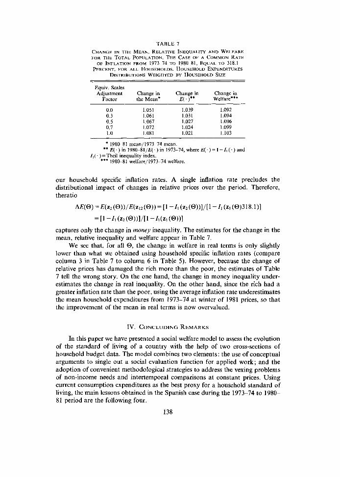
TABLE 7

Equiv. Scales Adjustment Change in Change in Change in

Factor the Mean* E(.)** Welfare***

* 1980-81 meanl1973-74 mean. ** E( . ) in 1980-81/E(.) in 1973-74, where E ( . ) = 1 - I , (.) and

I , ( . ) = Theil inequality index. *** 1980-8 1 welfare/ 1973-74 welfare.

our household specific inflation rates. A single inflation rate precludes the distributional impact of changes in relative prices over the period. Therefore, theratio

captures only the change in money inequality. The estimates for the change in the mean, relative inequality and welfare appear in Table 7.

We see that, for all 0, the change in welfare in real terms is only slightly lower than what we obtained using household specific inflation rates (compare column 3 in Table 7 to column 6 in Table 5). However, because the change of relative prices has damaged the rich more than the poor, the estimates of Table 7 tell the wrong story. On the one hand, the change in money inequality underestimates the change in real inequality. On the other hand, since the rich had a greater inflation rate than the poor, using the average inflation rate underestimates the mean household expenditures from 1973-74 at winter of 1981 prices, so that the improvement of the mean in real terms is now overvalued.

IV. CONCLUDING REMARKS

In this paper we have presented a social welfare model to assess the evolution of the standard of living of a country with the help of two cross-sections of household budget data. The model combines two elements: the use of conceptual arguments to single out a social evaluation function for applied work; and the adoption of convenient methodological strategies to address the vexing problems of non-income needs and interternporal comparisons at constant prices. Using current consumption expenditures as the best proxy for a household standard of living, the main lessons obtained in the Spanish case during the 1973-74 to 1980- 81 period are the following four.

(i) Intertemporal comparisons require the expression of original money income distributions at constant prices. The use of household specific price indices for this task permits the study of distributional implications of the changes in relative prices. With this aim in mind, we have used statistical price indices which provide convenient bounds for the true cost-of-living indices. We have presented the theoretical bounds for the change in the mean and inequality at prices of the initial and the final situation under comparison. Our empirical work shows that we can narrowly bound the corresponding theoretical magnitudes. Consequently, our estimates of welfare change are very robust to the choice of the reference price vector. We conclude that, at least in this case, we have been justified in avoiding the cost of estimating a complete demand system in order to recover the true cost-of-living household indices.

(ii) The construction of household specific inflation rates has paid some empirical dividends in this case. The reason is that we have found that the evolution of relative prices has damaged the rich more than the poor [see also Ruiz- Castillo (1995a)l. In a situation of this type, if we use a common inflation rate for all households we can be sure that our estimates of the inequality improvement would be biased downwards, while our estimates of the change in the mean would be biased upwards.

(iii) The separate study of each subgroup by partition into household size has been worthwhile. We have found considerable differences among them, but the use of decomposable measurement instruments allow us to understand how results at the household size level get translated to the population as a whole. In particular, given that larger households do worse than smaller ones, had we estimated the welfare change for the unweighted household distribution, we would have found a greater welfare improvement than with the household size weighted distribution in which each individual is assigned the adjusted expenditure of the household to which she belongs.

(iv) We have provided additional evidence on the usefulness of parametrizing the equivalence scales in the relative case when household size is assumed to be the only characteristic determining non-income needs. The extension of that model to the absolute case presented in this paper, has made possible the application of this notion which, in spite of its conceptual and practical interest, has been very seldom used in the empirical literature.

STATISTICAL APPENDIX TABLE A

MEAN HOUSEHOLD EXPENDITURES, RELATIVE INEQUALITY AND WELFARE FOR THE TOTAL POPULATION AT PRICES P~=WINTER 1981. HOUSEHOLD EXPENDITURES DISTRIBUTIONS

WEIGHTED BY HOUSEHOLD SIZE

1973-74 1980-8 1

0 Mean E ( . )* Welfare Mean E ( . ) * Welfare

0.0 93 1,092 0.7859 730,992 964,511 0.8320 802,505 0.3 590,187 0.8068 476,195 616,815 0.8490 523,667 0.5 439,452 0.8129 357,241 461,802 0.8525 393,676 0.7 329,717 0.8115 267,579 348,284 0.8489 295,671 1 .O 217,553 0.7938 172,695 23 1,477 0.8286 191,800

* E ( . ) = 1 - I , ( . ), where I , ( . ) =Theil inequality index.

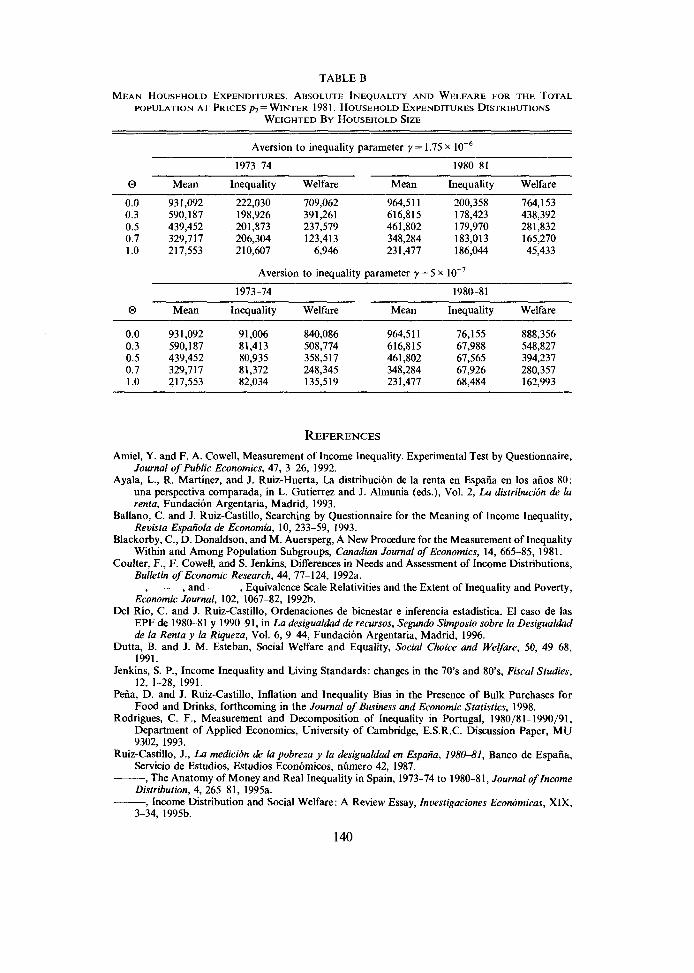
TABLE B

MEAN HOUSEHOLD EXPENDITURES, ABSOLUTE INEQUALITY AND WELFARE FOR THE TOTAL POPULATION AT PRICES p2= WINTER 1981. HOUSEHOLD EXPENDITURES DISTRIBUTIONS

WEIGHTED BY HOUSEHOLD SIZE

Aversion to inequality parameter y = 1.75 x

1973-74 1980-81

0 Mean Inequality Welfare Mean Inequality Welfare

Aversion to inequality parameter y = 5 x lo-'

0 Mean Inequality Welfare

0.0 931,092 91,006 840,086 0.3 590,187 81,413 508,774 0.5 439,452 80,935 358,517 0.7 329,717 81,372 248,345 1.0 217,553 82,034 135,519

Mean Inequality Welfare

964,511 76,155 888,356 616,815 67,988 548,827 461,802 67,565 394,237 348,284 67,926 280,357 231,477 68,484 162,993

Amiel, Y. and F. A. Cowell, Measurement of Income Inequality. Experimental Test by Questionnaire, Journal of Public Economics, 47, 3-26, 1992.

Ayala, L., R. Martinez, and J. Ruiz-Huerta, La distribucibn de la renta en Espaiia en 10s aiios 80: una perspectiva comparada, in L. Gutierrez and J. Almunia (eds.), Vol. 2, La distribucibn de la renta, Fundacibn Argentaria, Madrid, 1993.

Ballano, C. and J. Ruiz-Castillo, Searching by Questionnaire for the Meaning of Income Inequality, Reoista Espaiio[a de Economia, 10, 233-59, 1993.

Blackorby, C., D. Donaldson, and M. Auersperg, A New Procedure for the Measurement of Inequality Within and Among Population Subgroups, Canadian Journal of Economics, 14, 665-85, 1981.

Coulter, F., F. Cowell, and S. Jenkins, Differences in Needs and Assessment of Income Distributions, Bulletin of Economic Research, 44, 77-124, 1992a. -- , and -- , Equivalence Scale Relativities and the Extent of Inequality and Poverty,

Economic Journal, 102, 1067-82, 1992b. Del Rio, C. and J. Ruiz-Castillo, Ordenaciones de bienestar e inferencia estadistica. El caso de las

EPF de 1980-81 y 1990-91, in La desigualdad de recursos, Segundo Simposio sobre la Desigualdad de la Renta y la Riqueza, Vol. 6, 9-44, Fundaci6n Argentaria, Madrid, 1996.

Dutta, B. and J. M. Esteban, Social Welfare and Equality, Social Choice and Welfare, 50, 49-68, 1991.

Jenkins, S. P., Income Inequality and Living Standards: changes in the 70's and SO'S, Fiscal Studies, 12, 1-28, 1991.

Peiia, D. and J. Ruiz-Castillo, Inflation and Inequality Bias in the Presence of Bulk Purchases for Food and Drinks, forthcoming in the Journal of Business and Economic Statistics, 1998.

Rodrigues, C. F., Measurement and Decomposition of Inequality in Portugal, 1980/81-1990/91, Department of Applied Economics, University of Cambridge, E.S.R.C. Discussion Paper, MU 9302, 1993.

Ruiz-Castillo, J., La medicibn de la pobreza y la desigualdad en Espaiia, 198041, Banco de Espaiia, Servicio de Estudios, Estudios Econbmicos, numero 42, 1987.

-, The Anatomy of Money and Real Inequality in Spain, 1973-74 to 1980-81, Journal of Income Distribution, 4, 265-81, 1995a.

, Income Distribution and Social Welfare: A Review Essay, Investigaciones Economicas, XIX, 3-34, 1995b.

-, Caracteristicas geograficas y socioeconomicas en la evolution del nivel de vida en Espafia, 1973 74 a 1980-81, Hacienda Publica Espaiiola, 133, 145-69, 1995c.

Sanz, B., La articulacibn micro-macro en el sector hogares: de la Encuesta de Presupuestos Familiares a la Contabilidad National, in La desigualdad de recursos, II Simposio sobre la Desigualdad de la Renta y la Riqueza, Vol. 6, 45-86, Fundacion Argentaria, Madrid, 1996.

Sastre, M., Ensayos sobre la medicion de la desigualdad y el bienestar en tkrminos reales en Espafia, Ph.D. thesis, Universidad Complutense de Madrid, forthcoming, 1998.

Slesnick, D., The Standard of Living in the United States, Review of Income and Wealth, Series 37, Number 4, 363-86, 1991.

-, Gaining Ground: Poverty in the Postwar United States, Journal of Political Economy, 10, 1- 38, 1993.

A SIMPLIFIED MODEL FOR SOCIAL WELFARE ANALYSIS

Documents

Transcript of A SIMPLIFIED MODEL FOR SOCIAL WELFARE ANALYSIS