A Simple Framework for Contrastive Learning of Visual ... · A Simple Framework for Contrastive...
18
A Simple Framework for Contrastive Learning of Visual Representations Ting Chen 1 Simon Kornblith 1 Mohammad Norouzi 1 Geoffrey Hinton 1 Abstract This paper presents SimCLR: a simple framework for contrastive learning of visual representations. We simplify recently proposed contrastive self- supervised learning algorithms without requiring specialized architectures or a memory bank. In order to understand what enables the contrastive prediction tasks to learn useful representations, we systematically study the major components of our framework. We show that (1) composition of data augmentations plays a critical role in defining effective predictive tasks, (2) introducing a learn- able nonlinear transformation between the repre- sentation and the contrastive loss substantially im- proves the quality of the learned representations, and (3) contrastive learning benefits from larger batch sizes and more training steps compared to supervised learning. By combining these findings, we are able to considerably outperform previous methods for self-supervised and semi-supervised learning on ImageNet. A linear classifier trained on self-supervised representations learned by Sim- CLR achieves 76.5% top-1 accuracy, which is a 7% relative improvement over previous state-of- the-art, matching the performance of a supervised ResNet-50. When fine-tuned on only 1% of the labels, we achieve 85.8% top-5 accuracy, outper- forming AlexNet with 100× fewer labels. 1 1. Introduction Learning effective visual representations without human supervision is a long-standing problem. Most mainstream approaches fall into one of two classes: generative or dis- criminative. Generative approaches learn to generate or otherwise model pixels in the input space (Hinton et al., 2006; Kingma & Welling, 2013; Goodfellow et al., 2014). However, pixel-level generation is computationally expen- sive and may not be necessary for representation learning. 1 Google Research, Brain Team. Correspondence to: Ting Chen <[email protected]>. 1 Code available at https://github.com/google-research/simclr. Figure 1. ImageNet Top-1 accuracy of linear classifiers trained on representations learned with different self-supervised meth- ods (pretrained on ImageNet). Gray cross indicates supervised ResNet-50. Our method, SimCLR, is shown in bold. Discriminative approaches learn representations using objec- tive functions similar to those used for supervised learning, but train networks to perform pretext tasks where both the in- puts and labels are derived from an unlabeled dataset. Many such approaches have relied on heuristics to design pretext tasks (Doersch et al., 2015; Zhang et al., 2016; Noroozi & Favaro, 2016; Gidaris et al., 2018), which could limit the generality of the learned representations. Discriminative approaches based on contrastive learning in the latent space have recently shown great promise, achieving state-of-the- art results (Hadsell et al., 2006; Dosovitskiy et al., 2014; Oord et al., 2018; Bachman et al., 2019). In this work, we introduce a simple framework for con- trastive learning of visual representations, which we call SimCLR. Not only does SimCLR outperform previous work (Figure 1), but it is also simpler, requiring neither special- ized architectures (Bachman et al., 2019; Hénaff et al., 2019) nor a memory bank (Wu et al., 2018; Tian et al., 2019; He et al., 2019; Misra & van der Maaten, 2019). In order to understand what enables good contrastive repre- sentation learning, we systematically study the major com- ponents of our framework and show that: • Composition of multiple data augmentation operations is crucial in defining the contrastive prediction tasks that arXiv:2002.05709v2 [cs.LG] 30 Mar 2020
Transcript of A Simple Framework for Contrastive Learning of Visual ... · A Simple Framework for Contrastive...
A Simple Framework for Contrastive Learning of Visual Representations
Ting Chen 1 Simon Kornblith 1 Mohammad Norouzi 1 Geoffrey Hinton 1
AbstractThis paper presents SimCLR: a simple frameworkfor contrastive learning of visual representations.We simplify recently proposed contrastive self-supervised learning algorithms without requiringspecialized architectures or a memory bank. Inorder to understand what enables the contrastiveprediction tasks to learn useful representations,we systematically study the major components ofour framework. We show that (1) composition ofdata augmentations plays a critical role in definingeffective predictive tasks, (2) introducing a learn-able nonlinear transformation between the repre-sentation and the contrastive loss substantially im-proves the quality of the learned representations,and (3) contrastive learning benefits from largerbatch sizes and more training steps compared tosupervised learning. By combining these findings,we are able to considerably outperform previousmethods for self-supervised and semi-supervisedlearning on ImageNet. A linear classifier trainedon self-supervised representations learned by Sim-CLR achieves 76.5% top-1 accuracy, which is a7% relative improvement over previous state-of-the-art, matching the performance of a supervisedResNet-50. When fine-tuned on only 1% of thelabels, we achieve 85.8% top-5 accuracy, outper-forming AlexNet with 100× fewer labels. 1
1. IntroductionLearning effective visual representations without humansupervision is a long-standing problem. Most mainstreamapproaches fall into one of two classes: generative or dis-criminative. Generative approaches learn to generate orotherwise model pixels in the input space (Hinton et al.,2006; Kingma & Welling, 2013; Goodfellow et al., 2014).However, pixel-level generation is computationally expen-sive and may not be necessary for representation learning.
1Google Research, Brain Team. Correspondence to: Ting Chen<[email protected]>.
1Code available at https://github.com/google-research/simclr.
25 50 100 200 400 626Number of Parameters (Millions)
55
60
65
70
75
Imag
eNet
Top
-1 A
ccur
acy
(%)
InstDiscRotation
BigBiGAN
LA
CPCv2
CPCv2-L
CMCAMDIM
MoCo
MoCo (2x)
MoCo (4x)
PIRLPIRL-ens.
PIRL-c2xSimCLR
SimCLR (2x)
SimCLR (4x)Supervised
Figure 1. ImageNet Top-1 accuracy of linear classifiers trainedon representations learned with different self-supervised meth-ods (pretrained on ImageNet). Gray cross indicates supervisedResNet-50. Our method, SimCLR, is shown in bold.
Discriminative approaches learn representations using objec-tive functions similar to those used for supervised learning,but train networks to perform pretext tasks where both the in-puts and labels are derived from an unlabeled dataset. Manysuch approaches have relied on heuristics to design pretexttasks (Doersch et al., 2015; Zhang et al., 2016; Noroozi &Favaro, 2016; Gidaris et al., 2018), which could limit thegenerality of the learned representations. Discriminativeapproaches based on contrastive learning in the latent spacehave recently shown great promise, achieving state-of-the-art results (Hadsell et al., 2006; Dosovitskiy et al., 2014;Oord et al., 2018; Bachman et al., 2019).
In this work, we introduce a simple framework for con-trastive learning of visual representations, which we callSimCLR. Not only does SimCLR outperform previous work(Figure 1), but it is also simpler, requiring neither special-ized architectures (Bachman et al., 2019; Hénaff et al., 2019)nor a memory bank (Wu et al., 2018; Tian et al., 2019; Heet al., 2019; Misra & van der Maaten, 2019).
In order to understand what enables good contrastive repre-sentation learning, we systematically study the major com-ponents of our framework and show that:
• Composition of multiple data augmentation operationsis crucial in defining the contrastive prediction tasks that
arX
iv:2
002.
0570
9v2
[cs
.LG
] 3
0 M
ar 2
020
A Simple Framework for Contrastive Learning of Visual Representations
yield effective representations. In addition, unsupervisedcontrastive learning benefits from stronger data augmen-tation than supervised learning.
• Introducing a learnable nonlinear transformation be-tween the representation and the contrastive loss substan-tially improves the quality of the learned representations.
• Representation learning with contrastive cross entropyloss benefits from normalized embeddings and an appro-priately adjusted temperature parameter.
• Contrastive learning benefits from larger batch sizes andlonger training compared to its supervised counterpart.Like supervised learning, contrastive learning benefitsfrom deeper and wider networks.
We combine these findings to achieve a new state-of-the-artin self-supervised and semi-supervised learning on Ima-geNet ILSVRC-2012 (Russakovsky et al., 2015). Under thelinear evaluation protocol, SimCLR achieves 76.5% top-1accuracy, which is a 7% relative improvement over previousstate-of-the-art (Hénaff et al., 2019). When fine-tuned withonly 1% of the ImageNet labels, SimCLR achieves 85.8%top-5 accuracy, a relative improvement of 10% (Hénaff et al.,2019). When fine-tuned on other natural image classifica-tion datasets, SimCLR performs on par with or better thana strong supervised baseline (Kornblith et al., 2019) on 10out of 12 datasets.
2. Method2.1. The Contrastive Learning Framework
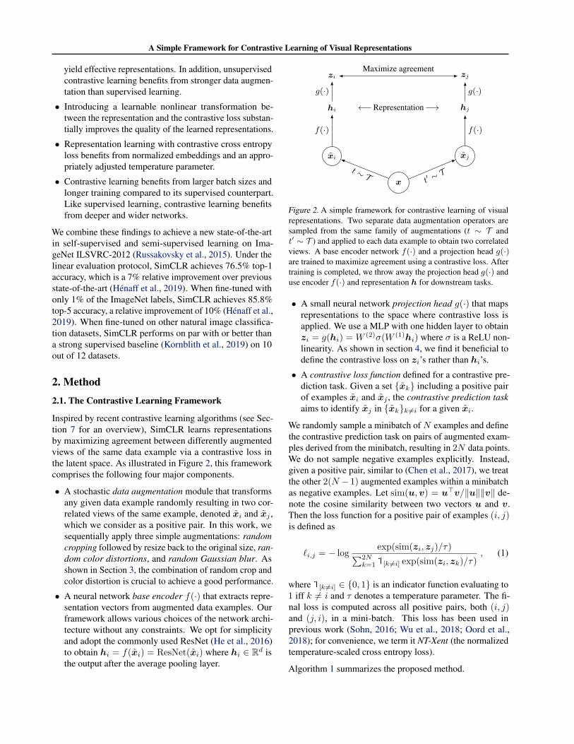
Inspired by recent contrastive learning algorithms (see Sec-tion 7 for an overview), SimCLR learns representationsby maximizing agreement between differently augmentedviews of the same data example via a contrastive loss inthe latent space. As illustrated in Figure 2, this frameworkcomprises the following four major components.
• A stochastic data augmentation module that transformsany given data example randomly resulting in two cor-related views of the same example, denoted x̃i and x̃j ,which we consider as a positive pair. In this work, wesequentially apply three simple augmentations: randomcropping followed by resize back to the original size, ran-dom color distortions, and random Gaussian blur. Asshown in Section 3, the combination of random crop andcolor distortion is crucial to achieve a good performance.
• A neural network base encoder f(·) that extracts repre-sentation vectors from augmented data examples. Ourframework allows various choices of the network archi-tecture without any constraints. We opt for simplicityand adopt the commonly used ResNet (He et al., 2016)to obtain hi = f(x̃i) = ResNet(x̃i) where hi ∈ Rd isthe output after the average pooling layer.
←−Representation−→
x
x̃i x̃j
hi hj
zi zj
t ∼ Tt′ ∼ T
f(·) f(·)
g(·) g(·)
Maximize agreement
Figure 2. A simple framework for contrastive learning of visualrepresentations. Two separate data augmentation operators aresampled from the same family of augmentations (t ∼ T andt′ ∼ T ) and applied to each data example to obtain two correlatedviews. A base encoder network f(·) and a projection head g(·)are trained to maximize agreement using a contrastive loss. Aftertraining is completed, we throw away the projection head g(·) anduse encoder f(·) and representation h for downstream tasks.
• A small neural network projection head g(·) that mapsrepresentations to the space where contrastive loss isapplied. We use a MLP with one hidden layer to obtainzi = g(hi) =W (2)σ(W (1)hi) where σ is a ReLU non-linearity. As shown in section 4, we find it beneficial todefine the contrastive loss on zi’s rather than hi’s.
• A contrastive loss function defined for a contrastive pre-diction task. Given a set {x̃k} including a positive pairof examples x̃i and x̃j , the contrastive prediction taskaims to identify x̃j in {x̃k}k 6=i for a given x̃i.
We randomly sample a minibatch of N examples and definethe contrastive prediction task on pairs of augmented exam-ples derived from the minibatch, resulting in 2N data points.We do not sample negative examples explicitly. Instead,given a positive pair, similar to (Chen et al., 2017), we treatthe other 2(N − 1) augmented examples within a minibatchas negative examples. Let sim(u,v) = u>v/‖u‖‖v‖ de-note the cosine similarity between two vectors u and v.Then the loss function for a positive pair of examples (i, j)is defined as
`i,j = − logexp(sim(zi, zj)/τ)∑2N
k=1 1[k 6=i] exp(sim(zi, zk)/τ), (1)
where 1[k 6=i] ∈ {0, 1} is an indicator function evaluating to1 iff k 6= i and τ denotes a temperature parameter. The fi-nal loss is computed across all positive pairs, both (i, j)and (j, i), in a mini-batch. This loss has been used inprevious work (Sohn, 2016; Wu et al., 2018; Oord et al.,2018); for convenience, we term it NT-Xent (the normalizedtemperature-scaled cross entropy loss).
Algorithm 1 summarizes the proposed method.
A Simple Framework for Contrastive Learning of Visual Representations
Algorithm 1 SimCLR’s main learning algorithm.
input: batch size N , constant τ , structure of f , g, T .for sampled minibatch {xk}Nk=1 do
for all k ∈ {1, . . . , N} dodraw two augmentation functions t∼T , t′∼T# the first augmentationx̃2k−1 = t(xk)h2k−1 = f(x̃2k−1) # representationz2k−1 = g(h2k−1) # projection# the second augmentationx̃2k = t′(xk)h2k = f(x̃2k) # representationz2k = g(h2k) # projection
end forfor all i ∈ {1, . . . , 2N} and j ∈ {1, . . . , 2N} dosi,j = z>i zj/(‖zi‖‖zj‖) # pairwise similarity
end fordefine `(i, j) as `(i, j)=− log
exp(si,j/τ)∑2Nk=1 1[k 6=i] exp(si,k/τ)
L = 12N
∑Nk=1 [`(2k−1, 2k) + `(2k, 2k−1)]
update networks f and g to minimize Lend forreturn encoder network f(·), and throw away g(·)
2.2. Training with Large Batch Size
We do not train the model with a memory bank (Wu et al.,2018). Instead, we vary the training batch size N from256 to 8192. A batch size of 8192 gives us 16382 negativeexamples per positive pair from both augmentation views.Training with large batch size may be unstable when usingstandard SGD/Momentum with linear learning rate scal-ing (Goyal et al., 2017). To stabilize the training, we use theLARS optimizer (You et al., 2017) for all batch sizes.Wetrain our model with Cloud TPUs, using 32 to 128 coresdepending on the batch size.2
Global BN. Standard ResNets use batch normaliza-tion (Ioffe & Szegedy, 2015). In distributed training withdata parallelism, the BN mean and variance are typicallyaggregated locally per device. In our contrastive learning,as positive pairs are computed in the same device, the modelcan exploit the local information leakage to improve pre-diction accuracy without improving representations. Weaddress this issue by aggregating BN mean and varianceover all devices during the training. Other approaches in-clude shuffling data examples (He et al., 2019), or replacingBN with layer norm (Hénaff et al., 2019).
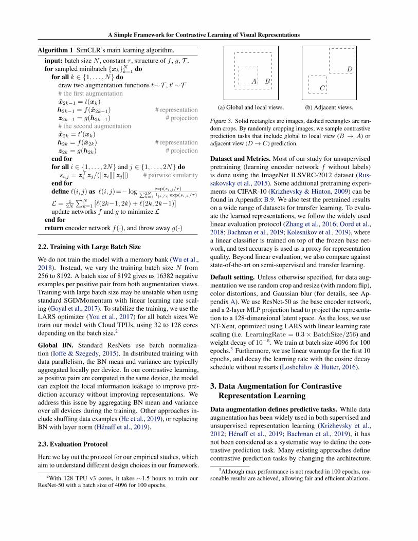
2.3. Evaluation Protocol
Here we lay out the protocol for our empirical studies, whichaim to understand different design choices in our framework.
2With 128 TPU v3 cores, it takes ∼1.5 hours to train ourResNet-50 with a batch size of 4096 for 100 epochs.
A B
(a) Global and local views.
C
D
(b) Adjacent views.
Figure 3. Solid rectangles are images, dashed rectangles are ran-dom crops. By randomly cropping images, we sample contrastiveprediction tasks that include global to local view (B → A) oradjacent view (D → C) prediction.
Dataset and Metrics. Most of our study for unsupervisedpretraining (learning encoder network f without labels)is done using the ImageNet ILSVRC-2012 dataset (Rus-sakovsky et al., 2015). Some additional pretraining experi-ments on CIFAR-10 (Krizhevsky & Hinton, 2009) can befound in Appendix B.9. We also test the pretrained resultson a wide range of datasets for transfer learning. To evalu-ate the learned representations, we follow the widely usedlinear evaluation protocol (Zhang et al., 2016; Oord et al.,2018; Bachman et al., 2019; Kolesnikov et al., 2019), wherea linear classifier is trained on top of the frozen base net-work, and test accuracy is used as a proxy for representationquality. Beyond linear evaluation, we also compare againststate-of-the-art on semi-supervised and transfer learning.
Default setting. Unless otherwise specified, for data aug-mentation we use random crop and resize (with random flip),color distortions, and Gaussian blur (for details, see Ap-pendix A). We use ResNet-50 as the base encoder network,and a 2-layer MLP projection head to project the representa-tion to a 128-dimensional latent space. As the loss, we useNT-Xent, optimized using LARS with linear learning ratescaling (i.e. LearningRate = 0.3 × BatchSize/256) andweight decay of 10−6. We train at batch size 4096 for 100epochs.3 Furthermore, we use linear warmup for the first 10epochs, and decay the learning rate with the cosine decayschedule without restarts (Loshchilov & Hutter, 2016).
3. Data Augmentation for ContrastiveRepresentation Learning
Data augmentation defines predictive tasks. While dataaugmentation has been widely used in both supervised andunsupervised representation learning (Krizhevsky et al.,2012; Hénaff et al., 2019; Bachman et al., 2019), it hasnot been considered as a systematic way to define the con-trastive prediction task. Many existing approaches definecontrastive prediction tasks by changing the architecture.
3Although max performance is not reached in 100 epochs, rea-sonable results are achieved, allowing fair and efficient ablations.
A Simple Framework for Contrastive Learning of Visual Representations
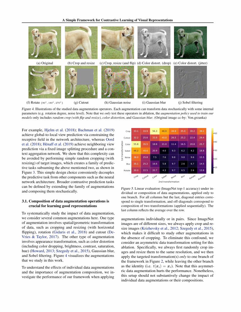
(a) Original (b) Crop and resize (c) Crop, resize (and flip) (d) Color distort. (drop) (e) Color distort. (jitter)
(f) Rotate {90◦, 180◦, 270◦} (g) Cutout (h) Gaussian noise (i) Gaussian blur (j) Sobel filtering
Figure 4. Illustrations of the studied data augmentation operators. Each augmentation can transform data stochastically with some internalparameters (e.g. rotation degree, noise level). Note that we only test these operators in ablation, the augmentation policy used to train ourmodels only includes random crop (with flip and resize), color distortion, and Gaussian blur. (Original image cc-by: Von.grzanka)
For example, Hjelm et al. (2018); Bachman et al. (2019)achieve global-to-local view prediction via constraining thereceptive field in the network architecture, whereas Oordet al. (2018); Hénaff et al. (2019) achieve neighboring viewprediction via a fixed image splitting procedure and a con-text aggregation network. We show that this complexity canbe avoided by performing simple random cropping (withresizing) of target images, which creates a family of predic-tive tasks subsuming the above mentioned two, as shown inFigure 3. This simple design choice conveniently decouplesthe predictive task from other components such as the neuralnetwork architecture. Broader contrastive prediction taskscan be defined by extending the family of augmentationsand composing them stochastically.
3.1. Composition of data augmentation operations iscrucial for learning good representations
To systematically study the impact of data augmentation,we consider several common augmentations here. One typeof augmentation involves spatial/geometric transformationof data, such as cropping and resizing (with horizontalflipping), rotation (Gidaris et al., 2018) and cutout (De-Vries & Taylor, 2017). The other type of augmentationinvolves appearance transformation, such as color distortion(including color dropping, brightness, contrast, saturation,hue) (Howard, 2013; Szegedy et al., 2015), Gaussian blur,and Sobel filtering. Figure 4 visualizes the augmentationsthat we study in this work.
To understand the effects of individual data augmentationsand the importance of augmentation composition, we in-vestigate the performance of our framework when applying
CropCutout
ColorSobel
Noise BlurRotate
Average
2nd transformation
Crop
Cutout
Color
Sobel
Noise
Blur
Rotate
1st t
rans
form
atio
n
33.1 33.9 56.3 46.0 39.9 35.0 30.2 39.2
32.2 25.6 33.9 40.0 26.5 25.2 22.4 29.4
55.8 35.5 18.8 21.0 11.4 16.5 20.8 25.7
46.2 40.6 20.9 4.0 9.3 6.2 4.2 18.8
38.8 25.8 7.5 7.6 9.8 9.8 9.6 15.5
35.1 25.2 16.6 5.8 9.7 2.6 6.7 14.5
30.0 22.5 20.7 4.3 9.7 6.5 2.6 13.810
20
30
40
50
Figure 5. Linear evaluation (ImageNet top-1 accuracy) under in-dividual or composition of data augmentations, applied only toone branch. For all columns but the last, diagonal entries corre-spond to single transformation, and off-diagonals correspond tocomposition of two transformations (applied sequentially). Thelast column reflects the average over the row.
augmentations individually or in pairs. Since ImageNetimages are of different sizes, we always apply crop and re-size images (Krizhevsky et al., 2012; Szegedy et al., 2015),which makes it difficult to study other augmentations inthe absence of cropping. To eliminate this confound, weconsider an asymmetric data transformation setting for thisablation. Specifically, we always first randomly crop im-ages and resize them to the same resolution, and we thenapply the targeted transformation(s) only to one branch ofthe framework in Figure 2, while leaving the other branchas the identity (i.e. t(xi) = xi). Note that this asymmet-ric data augmentation hurts the performance. Nonetheless,this setup should not substantively change the impact ofindividual data augmentations or their compositions.
A Simple Framework for Contrastive Learning of Visual Representations
(a) Without color distortion. (b) With color distortion.
Figure 6. Histograms of pixel intensities (over all channels) fordifferent crops of two different images (i.e. two rows). The imagefor the first row is from Figure 4. All axes have the same range.
Color distortion strengthMethods 1/8 1/4 1/2 1 1 (+Blur) AutoAug
SimCLR 59.6 61.0 62.6 63.2 64.5 61.1Supervised 77.0 76.7 76.5 75.7 75.4 77.1
Table 1. Top-1 accuracy of unsupervised ResNet-50 using linearevaluation and supervised ResNet-505, under varied color distor-tion strength (see Appendix A) and other data transformations.Strength 1 (+Blur) is our default data augmentation policy.
Figure 5 shows linear evaluation results under individualand composition of transformations. We observe that nosingle transformation suffices to learn good representations,even though the model can almost perfectly identify thepositive pairs in the contrastive task. When composing aug-mentations, the contrastive prediction task becomes harder,but the quality of representation improves dramatically.
One composition of augmentations stands out: random crop-ping and random color distortion. We conjecture that oneserious issue when using only random cropping as dataaugmentation is that most patches from an image share asimilar color distribution. Figure 6 shows that color his-tograms alone suffice to distinguish images. Neural netsmay exploit this shortcut to solve the predictive task. There-fore, it is critical to compose cropping with color distortionin order to learn generalizable features.
3.2. Contrastive learning needs stronger dataaugmentation than supervised learning
To further demonstrate the importance of the color aug-mentation, we adjust the strength of color augmentation asshown in Table 1. Stronger color augmentation substan-tially improves the linear evaluation of the learned unsuper-vised models. In this context, AutoAugment (Cubuk et al.,2019), a sophisticated augmentation policy found using su-pervised learning, does not work better than simple cropping+ (stronger) color distortion. When training supervised mod-
5Supervised models are trained for 90 epochs; longer trainingimproves performance of stronger augmentation by ∼ 0.5%.
0 50 100 150 200 250 300 350 400 450Number of Parameters (Millions)
50
55
60
65
70
75
80
Top
1 R101
R101(2x)
R152
R152(2x)
R18
R18(2x)
R18(4x)
R34
R34(2x)
R34(4x)
R50
R50(2x)
R50(4x)
Sup. R50Sup. R50(2x) Sup. R50(4x)
R50*
R50(2x)*R50(4x)*
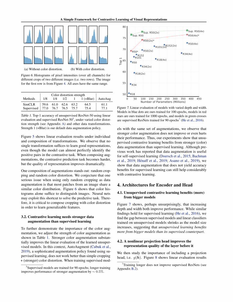
Figure 7. Linear evaluation of models with varied depth and width.Models in blue dots are ours trained for 100 epochs, models in redstars are ours trained for 1000 epochs, and models in green crossesare supervised ResNets trained for 90 epochs7 (He et al., 2016).
els with the same set of augmentations, we observe thatstronger color augmentation does not improve or even hurtstheir performance. Thus, our experiments show that unsu-pervised contrastive learning benefits from stronger (color)data augmentation than supervised learning. Although pre-vious work has reported that data augmentation is usefulfor self-supervised learning (Doersch et al., 2015; Bachmanet al., 2019; Hénaff et al., 2019; Asano et al., 2019), weshow that data augmentation that does not yield accuracybenefits for supervised learning can still help considerablywith contrastive learning.
4. Architectures for Encoder and Head4.1. Unsupervised contrastive learning benefits (more)
from bigger models
Figure 7 shows, perhaps unsurprisingly, that increasingdepth and width both improve performance. While similarfindings hold for supervised learning (He et al., 2016), wefind the gap between supervised models and linear classifierstrained on unsupervised models shrinks as the model sizeincreases, suggesting that unsupervised learning benefitsmore from bigger models than its supervised counterpart.
4.2. A nonlinear projection head improves therepresentation quality of the layer before it
We then study the importance of including a projectionhead, i.e. g(h). Figure 8 shows linear evaluation results
7Training longer does not improve supervised ResNets (seeAppendix B.2).
A Simple Framework for Contrastive Learning of Visual Representations
Name Negative loss function Gradient w.r.t. u
NT-Xent uTv+/τ − log∑
v∈{v+,v−} exp(uTv/τ) (1− exp(uT v+/τ)
Z(u))/τv+ −
∑v−
exp(uT v−/τ)Z(u)
/τv−
NT-Logistic log σ(uTv+/τ) + log σ(−uTv−/τ) (σ(−uTv+/τ))/τv+ − σ(uTv−/τ)/τv−
Margin Triplet −max(uTv− − uTv+ +m, 0) v+ − v− if uTv+ − uTv− < m else 0
Table 2. Negative loss functions and their gradients. All input vectors, i.e. u,v+,v−, are `2 normalized. NT-Xent is an abbreviation for“Normalized Temperature-scaled Cross Entropy”. Different loss functions impose different weightings of positive and negative examples.
32 64 128 256 5121024
2048
Projection output dimensionality
30
40
50
60
70
Top
1
ProjectionLinearNon-linearNone
Figure 8. Linear evaluation of representations with different pro-jection heads g(·) and various dimensions of z = g(h). Therepresentation h (before projection) is 2048-dimensional here.
What to predict? Random guess Representationh g(h)
Color vs grayscale 80 99.3 97.4Rotation 25 67.6 25.6Orig. vs corrupted 50 99.5 59.6Orig. vs Sobel filtered 50 96.6 56.3
Table 3. Accuracy of training additional MLPs on different repre-sentations to predict the transformation applied. Other than cropand color augmentation, we additionally and independently addrotation (one of {0◦, 90◦, 180◦, 270◦}), Gaussian noise, and So-bel filtering transformation during the pretraining for the last threerows. Both h and g(h) are of the same dimensionality, i.e. 2048.
using three different architecture for the head: (1) identitymapping; (2) linear projection, as used by several previousapproaches (Wu et al., 2018); and (3) the default nonlinearprojection with one additional hidden layer (and ReLU acti-vation), similar to Bachman et al. (2019). We observe that anonlinear projection is better than a linear projection (+3%),and much better than no projection (>10%). When a pro-jection head is used, similar results are observed regardlessof output dimension. Furthermore, even when nonlinearprojection is used, the layer before the projection head, h,is still much better (>10%) than the layer after, z = g(h),which shows that the hidden layer before the projectionhead is a better representation than the layer after.
We conjecture that the importance of using the representa-tion before the nonlinear projection is due to loss of informa-tion induced by the contrastive loss. In particular, z = g(h)is trained to be invariant to data transformation. Thus, g can
Margin NT-Logi. Margin (sh) NT-Logi.(sh) NT-Xent
50.9 51.6 57.5 57.9 63.9
Table 4. Linear evaluation (top-1) for models trained with differentloss functions. “sh” means using semi-hard negative mining.
`2 norm? τ Entropy Contrastive acc. Top 1
Yes
0.05 1.0 90.5 59.70.1 4.5 87.8 64.40.5 8.2 68.2 60.71 8.3 59.1 58.0
No 10 0.5 91.7 57.2100 0.5 92.1 57.0
Table 5. Linear evaluation for models trained with different choicesof `2 norm and temperature τ for NT-Xent loss. The contrastivedistribution is over 4096 examples.
remove information that may be useful for the downstreamtask, such as the color or orientation of objects. By leverag-ing the nonlinear transformation g(·), more information canbe formed and maintained in h. To verify this hypothesis,we conduct experiments that use either h or g(h) to learnto predict the transformation applied during the pretraining.Here we set g(h) = W (2)σ(W (1)h), with the same inputand output dimensionality (i.e. 2048). Table 3 shows hcontains much more information about the transformationapplied, while g(h) loses information.
5. Loss Functions and Batch Size5.1. Normalized cross entropy loss with adjustable
temperature works better than alternatives
We compare the NT-Xent loss against other commonly usedcontrastive loss functions, such as logistic loss (Mikolovet al., 2013), and margin loss (Schroff et al., 2015). Table 2shows the objective function as well as the gradient to theinput of the loss function. Looking at the gradient, we ob-serve 1) `2 normalization along with temperature effectivelyweights different examples, and an appropriate temperaturecan help the model learn from hard negatives; and 2) unlikecross-entropy, other objective functions do not weigh thenegatives by their relative hardness. As a result, one mustapply semi-hard negative mining (Schroff et al., 2015) for
A Simple Framework for Contrastive Learning of Visual Representations
100 200 300 400 500 600 700 800 900 1000Training epochs
50.0
52.5
55.0
57.5
60.0
62.5
65.0
67.5
70.0To
p 1
Batch size2565121024204840968192
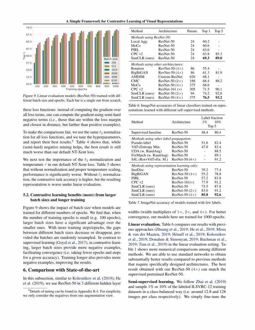
Figure 9. Linear evaluation models (ResNet-50) trained with dif-ferent batch size and epochs. Each bar is a single run from scratch.
these loss functions: instead of computing the gradient overall loss terms, one can compute the gradient using semi-hardnegative terms (i.e., those that are within the loss marginand closest in distance, but farther than positive examples).
To make the comparisons fair, we use the same `2 normaliza-tion for all loss functions, and we tune the hyperparameters,and report their best results.8 Table 4 shows that, while(semi-hard) negative mining helps, the best result is stillmuch worse than our default NT-Xent loss.
We next test the importance of the `2 normalization andtemperature τ in our default NT-Xent loss. Table 5 showsthat without normalization and proper temperature scaling,performance is significantly worse. Without `2 normaliza-tion, the contrastive task accuracy is higher, but the resultingrepresentation is worse under linear evaluation.
5.2. Contrastive learning benefits (more) from largerbatch sizes and longer training
Figure 9 shows the impact of batch size when models aretrained for different numbers of epochs. We find that, whenthe number of training epochs is small (e.g. 100 epochs),larger batch sizes have a significant advantage over thesmaller ones. With more training steps/epochs, the gapsbetween different batch sizes decrease or disappear, pro-vided the batches are randomly resampled. In contrast tosupervised learning (Goyal et al., 2017), in contrastive learn-ing, larger batch sizes provide more negative examples,facilitating convergence (i.e. taking fewer epochs and stepsfor a given accuracy). Training longer also provides morenegative examples, improving the results.
6. Comparison with State-of-the-artIn this subsection, similar to Kolesnikov et al. (2019); Heet al. (2019), we use ResNet-50 in 3 different hidden layer
8Details of tuning can be found in Appendix B.4. For simplicity,we only consider the negatives from one augmentation view.
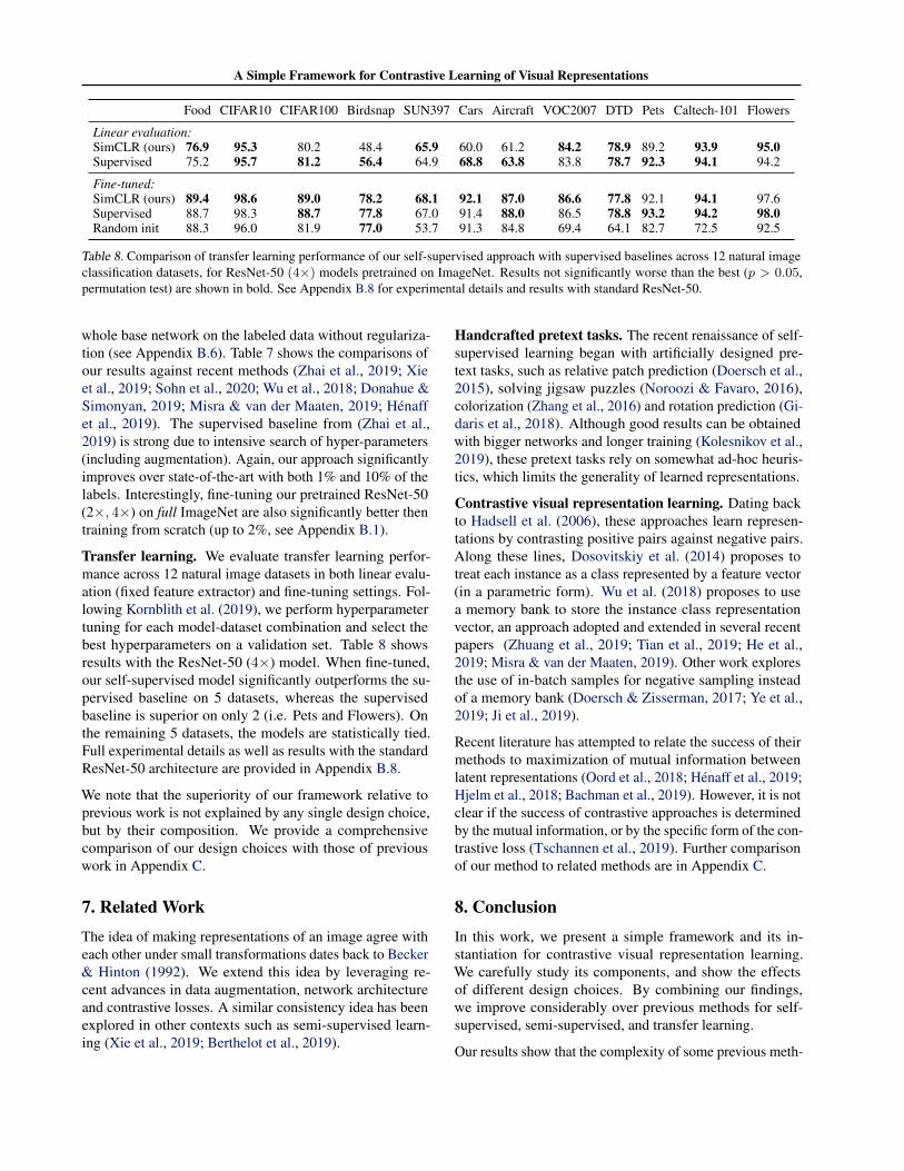
Method Architecture Param. Top 1 Top 5
Methods using ResNet-50:Local Agg. ResNet-50 24 60.2 -MoCo ResNet-50 24 60.6 -PIRL ResNet-50 24 63.6 -CPC v2 ResNet-50 24 63.8 85.3SimCLR (ours) ResNet-50 24 69.3 89.0
Methods using other architectures:Rotation RevNet-50 (4×) 86 55.4 -BigBiGAN RevNet-50 (4×) 86 61.3 81.9AMDIM Custom-ResNet 626 68.1 -CMC ResNet-50 (2×) 188 68.4 88.2MoCo ResNet-50 (4×) 375 68.6 -CPC v2 ResNet-161 (∗) 305 71.5 90.1SimCLR (ours) ResNet-50 (2×) 94 74.2 92.0SimCLR (ours) ResNet-50 (4×) 375 76.5 93.2
Table 6. ImageNet accuracies of linear classifiers trained on repre-sentations learned with different self-supervised methods.
Method ArchitectureLabel fraction1% 10%
Top 5
Supervised baseline ResNet-50 48.4 80.4
Methods using other label-propagation:Pseudo-label ResNet-50 51.6 82.4VAT+Entropy Min. ResNet-50 47.0 83.4UDA (w. RandAug) ResNet-50 - 88.5FixMatch (w. RandAug) ResNet-50 - 89.1S4L (Rot+VAT+En. M.) ResNet-50 (4×) - 91.2
Methods using representation learning only:InstDisc ResNet-50 39.2 77.4BigBiGAN RevNet-50 (4×) 55.2 78.8PIRL ResNet-50 57.2 83.8CPC v2 ResNet-161(∗) 77.9 91.2SimCLR (ours) ResNet-50 75.5 87.8SimCLR (ours) ResNet-50 (2×) 83.0 91.2SimCLR (ours) ResNet-50 (4×) 85.8 92.6
Table 7. ImageNet accuracy of models trained with few labels.
widths (width multipliers of 1×, 2×, and 4×). For betterconvergence, our models here are trained for 1000 epochs.
Linear evaluation. Table 6 compares our results with previ-ous approaches (Zhuang et al., 2019; He et al., 2019; Misra& van der Maaten, 2019; Hénaff et al., 2019; Kolesnikovet al., 2019; Donahue & Simonyan, 2019; Bachman et al.,2019; Tian et al., 2019) in the linear evaluation setting. Ta-ble 1 shows more numerical comparisons among differentmethods. We are able to use standard networks to obtainsubstantially better results compared to previous methodsthat require specifically designed architectures. The bestresult obtained with our ResNet-50 (4×) can match thesupervised pretrained ResNet-50.
Semi-supervised learning. We follow Zhai et al. (2019)and sample 1% or 10% of the labeled ILSVRC-12 trainingdatasets in a class-balanced way (i.e. around 12.8 and 128images per class respectively). We simply fine-tune the
A Simple Framework for Contrastive Learning of Visual Representations
Food CIFAR10 CIFAR100 Birdsnap SUN397 Cars Aircraft VOC2007 DTD Pets Caltech-101 Flowers
Linear evaluation:SimCLR (ours) 76.9 95.3 80.2 48.4 65.9 60.0 61.2 84.2 78.9 89.2 93.9 95.0Supervised 75.2 95.7 81.2 56.4 64.9 68.8 63.8 83.8 78.7 92.3 94.1 94.2
Fine-tuned:SimCLR (ours) 89.4 98.6 89.0 78.2 68.1 92.1 87.0 86.6 77.8 92.1 94.1 97.6Supervised 88.7 98.3 88.7 77.8 67.0 91.4 88.0 86.5 78.8 93.2 94.2 98.0Random init 88.3 96.0 81.9 77.0 53.7 91.3 84.8 69.4 64.1 82.7 72.5 92.5
Table 8. Comparison of transfer learning performance of our self-supervised approach with supervised baselines across 12 natural imageclassification datasets, for ResNet-50 (4×) models pretrained on ImageNet. Results not significantly worse than the best (p > 0.05,permutation test) are shown in bold. See Appendix B.8 for experimental details and results with standard ResNet-50.
whole base network on the labeled data without regulariza-tion (see Appendix B.6). Table 7 shows the comparisons ofour results against recent methods (Zhai et al., 2019; Xieet al., 2019; Sohn et al., 2020; Wu et al., 2018; Donahue &Simonyan, 2019; Misra & van der Maaten, 2019; Hénaffet al., 2019). The supervised baseline from (Zhai et al.,2019) is strong due to intensive search of hyper-parameters(including augmentation). Again, our approach significantlyimproves over state-of-the-art with both 1% and 10% of thelabels. Interestingly, fine-tuning our pretrained ResNet-50(2×, 4×) on full ImageNet are also significantly better thentraining from scratch (up to 2%, see Appendix B.1).
Transfer learning. We evaluate transfer learning perfor-mance across 12 natural image datasets in both linear evalu-ation (fixed feature extractor) and fine-tuning settings. Fol-lowing Kornblith et al. (2019), we perform hyperparametertuning for each model-dataset combination and select thebest hyperparameters on a validation set. Table 8 showsresults with the ResNet-50 (4×) model. When fine-tuned,our self-supervised model significantly outperforms the su-pervised baseline on 5 datasets, whereas the supervisedbaseline is superior on only 2 (i.e. Pets and Flowers). Onthe remaining 5 datasets, the models are statistically tied.Full experimental details as well as results with the standardResNet-50 architecture are provided in Appendix B.8.
We note that the superiority of our framework relative toprevious work is not explained by any single design choice,but by their composition. We provide a comprehensivecomparison of our design choices with those of previouswork in Appendix C.
7. Related WorkThe idea of making representations of an image agree witheach other under small transformations dates back to Becker& Hinton (1992). We extend this idea by leveraging re-cent advances in data augmentation, network architectureand contrastive losses. A similar consistency idea has beenexplored in other contexts such as semi-supervised learn-ing (Xie et al., 2019; Berthelot et al., 2019).
Handcrafted pretext tasks. The recent renaissance of self-supervised learning began with artificially designed pre-text tasks, such as relative patch prediction (Doersch et al.,2015), solving jigsaw puzzles (Noroozi & Favaro, 2016),colorization (Zhang et al., 2016) and rotation prediction (Gi-daris et al., 2018). Although good results can be obtainedwith bigger networks and longer training (Kolesnikov et al.,2019), these pretext tasks rely on somewhat ad-hoc heuris-tics, which limits the generality of learned representations.
Contrastive visual representation learning. Dating backto Hadsell et al. (2006), these approaches learn represen-tations by contrasting positive pairs against negative pairs.Along these lines, Dosovitskiy et al. (2014) proposes totreat each instance as a class represented by a feature vector(in a parametric form). Wu et al. (2018) proposes to usea memory bank to store the instance class representationvector, an approach adopted and extended in several recentpapers (Zhuang et al., 2019; Tian et al., 2019; He et al.,2019; Misra & van der Maaten, 2019). Other work exploresthe use of in-batch samples for negative sampling insteadof a memory bank (Doersch & Zisserman, 2017; Ye et al.,2019; Ji et al., 2019).
Recent literature has attempted to relate the success of theirmethods to maximization of mutual information betweenlatent representations (Oord et al., 2018; Hénaff et al., 2019;Hjelm et al., 2018; Bachman et al., 2019). However, it is notclear if the success of contrastive approaches is determinedby the mutual information, or by the specific form of the con-trastive loss (Tschannen et al., 2019). Further comparisonof our method to related methods are in Appendix C.
8. ConclusionIn this work, we present a simple framework and its in-stantiation for contrastive visual representation learning.We carefully study its components, and show the effectsof different design choices. By combining our findings,we improve considerably over previous methods for self-supervised, semi-supervised, and transfer learning.
Our results show that the complexity of some previous meth-
A Simple Framework for Contrastive Learning of Visual Representations
ods for self-supervised learning is not necessary to achievegood performance. Our approach differs from standard su-pervised learning on ImageNet only in the choice of dataaugmentation, the use of a nonlinear head at the end of thenetwork, and the loss function. The strength of this simpleframework suggests that, despite a recent surge in interest,self-supervised learning remains undervalued.
AcknowledgementsWe would like to thank Xiaohua Zhai, Rafael Müller andYani Ioannou for their feedback on the draft. We are alsograteful for general support from Google Research teams inToronto and elsewhere.
ReferencesAsano, Y. M., Rupprecht, C., and Vedaldi, A. A critical analysis
of self-supervision, or what we can learn from a single image.arXiv preprint arXiv:1904.13132, 2019.
Bachman, P., Hjelm, R. D., and Buchwalter, W. Learning rep-resentations by maximizing mutual information across views.In Advances in Neural Information Processing Systems, pp.15509–15519, 2019.
Becker, S. and Hinton, G. E. Self-organizing neural network thatdiscovers surfaces in random-dot stereograms. Nature, 355(6356):161–163, 1992.
Berg, T., Liu, J., Lee, S. W., Alexander, M. L., Jacobs, D. W.,and Belhumeur, P. N. Birdsnap: Large-scale fine-grained visualcategorization of birds. In IEEE Conference on Computer Visionand Pattern Recognition (CVPR), pp. 2019–2026. IEEE, 2014.
Berthelot, D., Carlini, N., Goodfellow, I., Papernot, N., Oliver,A., and Raffel, C. A. Mixmatch: A holistic approach to semi-supervised learning. In Advances in Neural Information Pro-cessing Systems, pp. 5050–5060, 2019.
Bossard, L., Guillaumin, M., and Van Gool, L. Food-101–miningdiscriminative components with random forests. In Europeanconference on computer vision, pp. 446–461. Springer, 2014.
Chen, T., Sun, Y., Shi, Y., and Hong, L. On sampling strategiesfor neural network-based collaborative filtering. In Proceed-ings of the 23rd ACM SIGKDD International Conference onKnowledge Discovery and Data Mining, pp. 767–776, 2017.
Cimpoi, M., Maji, S., Kokkinos, I., Mohamed, S., and Vedaldi,A. Describing textures in the wild. In IEEE Conference onComputer Vision and Pattern Recognition (CVPR), pp. 3606–3613. IEEE, 2014.
Cubuk, E. D., Zoph, B., Mane, D., Vasudevan, V., and Le, Q. V.Autoaugment: Learning augmentation strategies from data. InProceedings of the IEEE conference on computer vision andpattern recognition, pp. 113–123, 2019.
DeVries, T. and Taylor, G. W. Improved regularization ofconvolutional neural networks with cutout. arXiv preprintarXiv:1708.04552, 2017.
Doersch, C. and Zisserman, A. Multi-task self-supervised visuallearning. In Proceedings of the IEEE International Conferenceon Computer Vision, pp. 2051–2060, 2017.
Doersch, C., Gupta, A., and Efros, A. A. Unsupervised visualrepresentation learning by context prediction. In Proceedingsof the IEEE International Conference on Computer Vision, pp.1422–1430, 2015.
Donahue, J. and Simonyan, K. Large scale adversarial representa-tion learning. In Advances in Neural Information ProcessingSystems, pp. 10541–10551, 2019.
Donahue, J., Jia, Y., Vinyals, O., Hoffman, J., Zhang, N., Tzeng, E.,and Darrell, T. Decaf: A deep convolutional activation featurefor generic visual recognition. In International Conference onMachine Learning, pp. 647–655, 2014.
Dosovitskiy, A., Springenberg, J. T., Riedmiller, M., and Brox, T.Discriminative unsupervised feature learning with convolutionalneural networks. In Advances in neural information processingsystems, pp. 766–774, 2014.
Everingham, M., Van Gool, L., Williams, C. K., Winn, J., andZisserman, A. The pascal visual object classes (voc) challenge.International Journal of Computer Vision, 88(2):303–338, 2010.
Fei-Fei, L., Fergus, R., and Perona, P. Learning generative visualmodels from few training examples: An incremental bayesianapproach tested on 101 object categories. In IEEE Conferenceon Computer Vision and Pattern Recognition (CVPR) Workshopon Generative-Model Based Vision, 2004.
Gidaris, S., Singh, P., and Komodakis, N. Unsupervised represen-tation learning by predicting image rotations. arXiv preprintarXiv:1803.07728, 2018.
Goodfellow, I., Pouget-Abadie, J., Mirza, M., Xu, B., Warde-Farley, D., Ozair, S., Courville, A., and Bengio, Y. Generativeadversarial nets. In Advances in neural information processingsystems, pp. 2672–2680, 2014.
Goyal, P., Dollár, P., Girshick, R., Noordhuis, P., Wesolowski, L.,Kyrola, A., Tulloch, A., Jia, Y., and He, K. Accurate, largeminibatch sgd: Training imagenet in 1 hour. arXiv preprintarXiv:1706.02677, 2017.
Hadsell, R., Chopra, S., and LeCun, Y. Dimensionality reductionby learning an invariant mapping. In 2006 IEEE Computer So-ciety Conference on Computer Vision and Pattern Recognition(CVPR’06), volume 2, pp. 1735–1742. IEEE, 2006.
He, K., Zhang, X., Ren, S., and Sun, J. Deep residual learning forimage recognition. In Proceedings of the IEEE conference oncomputer vision and pattern recognition, pp. 770–778, 2016.
He, K., Fan, H., Wu, Y., Xie, S., and Girshick, R. Momentumcontrast for unsupervised visual representation learning. arXivpreprint arXiv:1911.05722, 2019.
Hénaff, O. J., Razavi, A., Doersch, C., Eslami, S., and Oord, A.v. d. Data-efficient image recognition with contrastive predictivecoding. arXiv preprint arXiv:1905.09272, 2019.
Hinton, G. E., Osindero, S., and Teh, Y.-W. A fast learning al-gorithm for deep belief nets. Neural computation, 18(7):1527–1554, 2006.
A Simple Framework for Contrastive Learning of Visual Representations
Hjelm, R. D., Fedorov, A., Lavoie-Marchildon, S., Grewal, K.,Bachman, P., Trischler, A., and Bengio, Y. Learning deep repre-sentations by mutual information estimation and maximization.arXiv preprint arXiv:1808.06670, 2018.
Howard, A. G. Some improvements on deep convolutionalneural network based image classification. arXiv preprintarXiv:1312.5402, 2013.
Ioffe, S. and Szegedy, C. Batch normalization: Accelerating deepnetwork training by reducing internal covariate shift. arXivpreprint arXiv:1502.03167, 2015.
Ji, X., Henriques, J. F., and Vedaldi, A. Invariant informationclustering for unsupervised image classification and segmenta-tion. In Proceedings of the IEEE International Conference onComputer Vision, pp. 9865–9874, 2019.
Kingma, D. P. and Welling, M. Auto-encoding variational bayes.arXiv preprint arXiv:1312.6114, 2013.
Kolesnikov, A., Zhai, X., and Beyer, L. Revisiting self-supervisedvisual representation learning. In Proceedings of the IEEEconference on Computer Vision and Pattern Recognition, pp.1920–1929, 2019.
Kornblith, S., Shlens, J., and Le, Q. V. Do better ImageNet modelstransfer better? In Proceedings of the IEEE conference oncomputer vision and pattern recognition, pp. 2661–2671, 2019.
Krause, J., Deng, J., Stark, M., and Fei-Fei, L. Collecting alarge-scale dataset of fine-grained cars. In Second Workshop onFine-Grained Visual Categorization, 2013.
Krizhevsky, A. and Hinton, G. Learning multiple layers of featuresfrom tiny images. Technical report, University of Toronto,2009. URL https://www.cs.toronto.edu/~kriz/learning-features-2009-TR.pdf.
Krizhevsky, A., Sutskever, I., and Hinton, G. E. Imagenet classifi-cation with deep convolutional neural networks. In Advances inneural information processing systems, pp. 1097–1105, 2012.
Loshchilov, I. and Hutter, F. Sgdr: Stochastic gradient descentwith warm restarts. arXiv preprint arXiv:1608.03983, 2016.
Maaten, L. v. d. and Hinton, G. Visualizing data using t-sne. Jour-nal of machine learning research, 9(Nov):2579–2605, 2008.
Maji, S., Kannala, J., Rahtu, E., Blaschko, M., and Vedaldi, A.Fine-grained visual classification of aircraft. Technical report,2013.
Mikolov, T., Chen, K., Corrado, G., and Dean, J. Efficient esti-mation of word representations in vector space. arXiv preprintarXiv:1301.3781, 2013.
Misra, I. and van der Maaten, L. Self-supervised learn-ing of pretext-invariant representations. arXiv preprintarXiv:1912.01991, 2019.
Nilsback, M.-E. and Zisserman, A. Automated flower classificationover a large number of classes. In Computer Vision, Graphics &Image Processing, 2008. ICVGIP’08. Sixth Indian Conferenceon, pp. 722–729. IEEE, 2008.
Noroozi, M. and Favaro, P. Unsupervised learning of visual repre-sentations by solving jigsaw puzzles. In European Conferenceon Computer Vision, pp. 69–84. Springer, 2016.
Oord, A. v. d., Li, Y., and Vinyals, O. Representation learning withcontrastive predictive coding. arXiv preprint arXiv:1807.03748,2018.
Parkhi, O. M., Vedaldi, A., Zisserman, A., and Jawahar, C. Catsand dogs. In IEEE Conference on Computer Vision and PatternRecognition (CVPR), pp. 3498–3505. IEEE, 2012.
Russakovsky, O., Deng, J., Su, H., Krause, J., Satheesh, S., Ma,S., Huang, Z., Karpathy, A., Khosla, A., Bernstein, M., et al.Imagenet large scale visual recognition challenge. Internationaljournal of computer vision, 115(3):211–252, 2015.
Schroff, F., Kalenichenko, D., and Philbin, J. Facenet: A unifiedembedding for face recognition and clustering. In Proceed-ings of the IEEE conference on computer vision and patternrecognition, pp. 815–823, 2015.
Simonyan, K. and Zisserman, A. Very deep convolutionalnetworks for large-scale image recognition. arXiv preprintarXiv:1409.1556, 2014.
Sohn, K. Improved deep metric learning with multi-class n-pairloss objective. In Advances in neural information processingsystems, pp. 1857–1865, 2016.
Sohn, K., Berthelot, D., Li, C.-L., Zhang, Z., Carlini, N., Cubuk,E. D., Kurakin, A., Zhang, H., and Raffel, C. Fixmatch: Simpli-fying semi-supervised learning with consistency and confidence.arXiv preprint arXiv:2001.07685, 2020.
Szegedy, C., Liu, W., Jia, Y., Sermanet, P., Reed, S., Anguelov, D.,Erhan, D., Vanhoucke, V., and Rabinovich, A. Going deeperwith convolutions. In Proceedings of the IEEE conference oncomputer vision and pattern recognition, pp. 1–9, 2015.
Tian, Y., Krishnan, D., and Isola, P. Contrastive multiview coding.arXiv preprint arXiv:1906.05849, 2019.
Tschannen, M., Djolonga, J., Rubenstein, P. K., Gelly, S., and Lu-cic, M. On mutual information maximization for representationlearning. arXiv preprint arXiv:1907.13625, 2019.
Wu, Z., Xiong, Y., Yu, S. X., and Lin, D. Unsupervised featurelearning via non-parametric instance discrimination. In Proceed-ings of the IEEE Conference on Computer Vision and PatternRecognition, pp. 3733–3742, 2018.
Xiao, J., Hays, J., Ehinger, K. A., Oliva, A., and Torralba, A. Sundatabase: Large-scale scene recognition from abbey to zoo. InIEEE Conference on Computer Vision and Pattern Recognition(CVPR), pp. 3485–3492. IEEE, 2010.
Xie, Q., Dai, Z., Hovy, E., Luong, M.-T., and Le, Q. V. Unsu-pervised data augmentation. arXiv preprint arXiv:1904.12848,2019.
Ye, M., Zhang, X., Yuen, P. C., and Chang, S.-F. Unsupervisedembedding learning via invariant and spreading instance feature.In Proceedings of the IEEE Conference on Computer Visionand Pattern Recognition, pp. 6210–6219, 2019.
You, Y., Gitman, I., and Ginsburg, B. Large batch training of con-volutional networks. arXiv preprint arXiv:1708.03888, 2017.
Zhai, X., Oliver, A., Kolesnikov, A., and Beyer, L. S4l: Self-supervised semi-supervised learning. In The IEEE InternationalConference on Computer Vision (ICCV), October 2019.

A Simple Framework for Contrastive Learning of Visual Representations
Zhang, R., Isola, P., and Efros, A. A. Colorful image coloriza-tion. In European conference on computer vision, pp. 649–666.Springer, 2016.
Zhuang, C., Zhai, A. L., and Yamins, D. Local aggregation forunsupervised learning of visual embeddings. In Proceedingsof the IEEE International Conference on Computer Vision, pp.6002–6012, 2019.
A Simple Framework for Contrastive Learning of Visual Representations
A. Data Augmentation DetailsIn our default pre-training setting (which is used to train our best models), we utilize random crop (with resize and randomflip), random color distortion, and random Gaussian blur as the data augmentations. The details of these three augmentationsare provided below.
Random crop and resize to 224x224 We use standard Inception-style random cropping (Szegedy et al., 2015). Thecrop of random size (uniform from 0.08 to 1.0 in area) of the original size and a random aspect ratio (default: of3/4 to 4/3) of the original aspect ratio is made. This crop is finally resized to the original size. This has been imple-mented in Tensorflow as “slim.preprocessing.inception_preprocessing.distorted_bounding_box_crop”, or in Pytorchas “torchvision.transforms.RandomResizedCrop”. Additionally, the random crop (with resize) is always followed by arandom horizontal/left-to-right flip with 50% probability. This is helpful but not essential. By removing this from our defaultaugmentation policy, the top-1 linear evaluation drops from 64.5% to 63.4% for our ResNet-50 model trained in 100 epochs.
Color distortion Color distortion is composed by color jittering and color dropping. We find stronger color jitteringusually helps, so we set a strength parameter.
A pseudo-code for color distortion using TensorFlow is as follows.
import tensorflow as tfdef color_distortion(image, s=1.0):
# image is a tensor with value range in [0, 1].# s is the strength of color distortion.
def color_jitter(x):# one can also shuffle the order of following augmentations# each time they are applied.x = tf.image.random_brightness(x, max_delta=0.8*s)x = tf.image.random_contrast(x, lower=1-0.8*s, upper=1+0.8*s)x = tf.image.random_saturation(x, lower=1-0.8*s, upper=1+0.8*s)x = tf.image.random_hue(x, max_delta=0.2*s)x = tf.clip_by_value(x, 0, 1)return x
def color_drop(x):image = tf.image.rgb_to_grayscale(image)image = tf.tile(image, [1, 1, 3])
# randomly apply transformation with probability p.image = random_apply(color_jitter, image, p=0.8)image = random_apply(color_drop, image, p=0.2)return image
A pseudo-code for color distortion using Pytorch is as follows 9.
from torchvision import transformsdef get_color_distortion(s=1.0):
# s is the strength of color distortion.color_jitter = transforms.ColorJitter(0.8*s, 0.8*s, 0.8*s, 0.2*s)rnd_color_jitter = transforms.RandomApply([color_jitter], p=0.8)rnd_gray = transforms.RandomGrayscale(p=0.2)color_distort = transforms.Compose([
rnd_color_jitter,rnd_gray])
9Our code and results are based on Tensorflow, the Pytorch code here is a reference.
A Simple Framework for Contrastive Learning of Visual Representations
return color_distort
Gaussian blur This augmentation is in our default policy. We find it helpful, as it improves our ResNet-50 trained for100 epochs from 63.2% to 64.5%. We blur the image 50% of the time using a Gaussian kernel. We randomly sampleσ ∈ [0.1, 2.0], and the kernel size is set to be 10% of the image height/width.
B. Additional Experimental ResultsB.1. Broader composition of data augmentations further improves performance
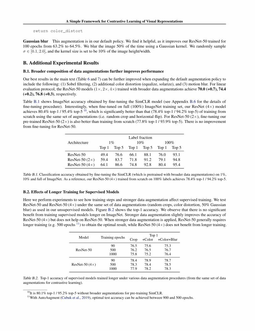
Our best results in the main text (Table 6 and 7) can be further improved when expanding the default augmentation policy toinclude the following: (1) Sobel filtering, (2) additional color distortion (equalize, solarize), and (3) motion blur. For linearevaluation protocol, the ResNet-50 models (1×, 2×, 4×) trained with broader data augmentations achieve 70.0 (+0.7), 74.4(+0.2), 76.8 (+0.3), respectively.
Table B.1 shows ImageNet accuracy obtained by fine-tuning the SimCLR model (see Appendix B.6 for the details offine-tuning procedure). Interestingly, when fine-tuned on full (100%) ImageNet training set, our ResNet (4×) modelachieves 80.4% top-1 / 95.4% top-5 10, which is significantly better than that (78.4% top-1 / 94.2% top-5) of training fromscratch using the same set of augmentations (i.e. random crop and horizontal flip). For ResNet-50 (2×), fine-tuning ourpre-trained ResNet-50 (2×) is also better than training from scratch (77.8% top-1 / 93.9% top-5). There is no improvementfrom fine-tuning for ResNet-50.
ArchitectureLabel fraction
1% 10% 100%Top 1 Top 5 Top 1 Top 5 Top 1 Top 5
ResNet-50 49.4 76.6 66.1 88.1 76.0 93.1ResNet-50 (2×) 59.4 83.7 71.8 91.2 79.1 94.8ResNet-50 (4×) 64.1 86.6 74.8 92.8 80.4 95.4
Table B.1. Classification accuracy obtained by fine-tuning the SimCLR (which is pretrained with broader data augmentations) on 1%,10% and full of ImageNet. As a reference, our ResNet-50 (4×) trained from scratch on 100% labels achieves 78.4% top-1 / 94.2% top-5.
B.2. Effects of Longer Training for Supervised Models
Here we perform experiments to see how training steps and stronger data augmentation affect supervised training. We testResNet-50 and ResNet-50 (4×) under the same set of data augmentations (random crops, color distortion, 50% Gaussianblur) as used in our unsupervised models. Figure B.2 shows the top-1 accuracy. We observe that there is no significantbenefit from training supervised models longer on ImageNet. Stronger data augmentation slightly improves the accuracy ofResNet-50 (4×) but does not help on ResNet-50. When stronger data augmentation is applied, ResNet-50 generally requireslonger training (e.g. 500 epochs 11) to obtain the optimal result, while ResNet-50 (4×) does not benefit from longer training.
Model Training epochs Top 1Crop +Color +Color+Blur
ResNet-5090 76.5 75.6 75.3500 76.2 76.5 76.7
1000 75.8 75.2 76.4
ResNet-50 (4×)90 78.4 78.9 78.7500 78.3 78.4 78.5
1000 77.9 78.2 78.3
Table B.2. Top-1 accuracy of supervised models trained longer under various data augmentation procedures (from the same set of dataaugmentations for contrastive learning).
10It is 80.1% top-1 / 95.2% top-5 without broader augmentations for pre-training SimCLR.11With AutoAugment (Cubuk et al., 2019), optimal test accuracy can be achieved between 900 and 500 epochs.
A Simple Framework for Contrastive Learning of Visual Representations
B.3. Understanding The Non-Linear Projection Head
0 500 1000 1500 2000Ranking
0
2
4
6
8
10
12
14
16
Squa
red
eige
nval
ue
(a) Y-axis in uniform scale.
0 500 1000 1500 2000Ranking
10−11
10−9
10−7
10−5
10−3
10−1
101
Squa
red
eige
nval
ue
(b) Y-axis in log scale.
Figure B.1. Squared real eigenvalue distribution of linear projectionmatrix W ∈ R2048×2048 used to compute g(h) =Wh.
(a) h (b) z = g(h)
Figure B.2. t-SNE visualizations of hidden vectors of images froma randomly selected 10 classes in the validation set.
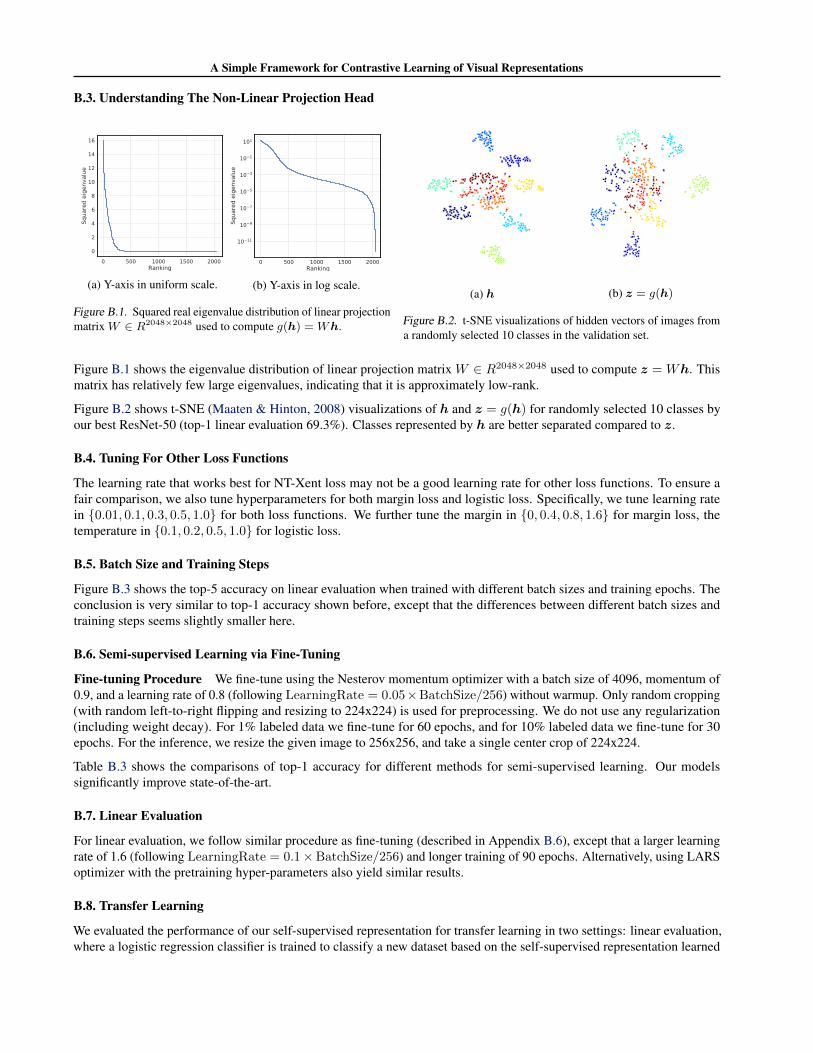
Figure B.1 shows the eigenvalue distribution of linear projection matrix W ∈ R2048×2048 used to compute z =Wh. Thismatrix has relatively few large eigenvalues, indicating that it is approximately low-rank.
Figure B.2 shows t-SNE (Maaten & Hinton, 2008) visualizations of h and z = g(h) for randomly selected 10 classes byour best ResNet-50 (top-1 linear evaluation 69.3%). Classes represented by h are better separated compared to z.
B.4. Tuning For Other Loss Functions
The learning rate that works best for NT-Xent loss may not be a good learning rate for other loss functions. To ensure afair comparison, we also tune hyperparameters for both margin loss and logistic loss. Specifically, we tune learning ratein {0.01, 0.1, 0.3, 0.5, 1.0} for both loss functions. We further tune the margin in {0, 0.4, 0.8, 1.6} for margin loss, thetemperature in {0.1, 0.2, 0.5, 1.0} for logistic loss.
B.5. Batch Size and Training Steps
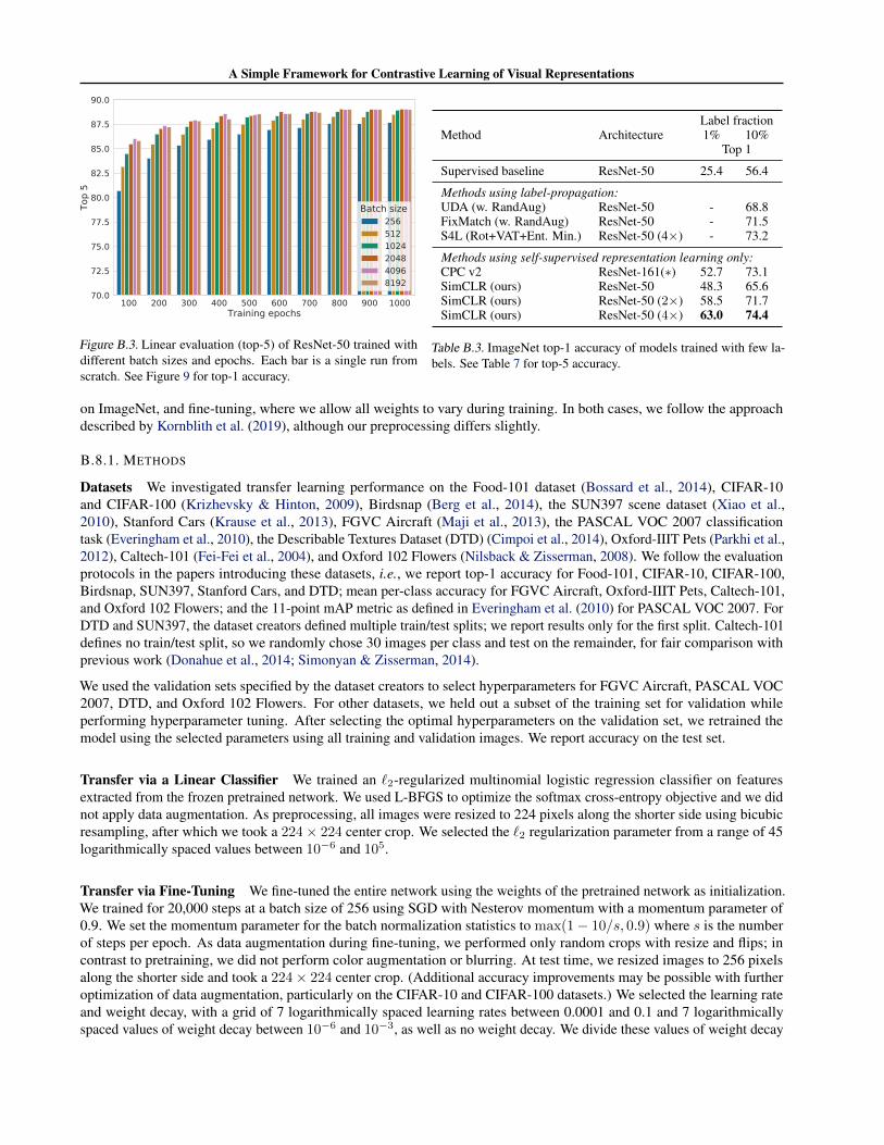
Figure B.3 shows the top-5 accuracy on linear evaluation when trained with different batch sizes and training epochs. Theconclusion is very similar to top-1 accuracy shown before, except that the differences between different batch sizes andtraining steps seems slightly smaller here.
B.6. Semi-supervised Learning via Fine-Tuning
Fine-tuning Procedure We fine-tune using the Nesterov momentum optimizer with a batch size of 4096, momentum of0.9, and a learning rate of 0.8 (following LearningRate = 0.05×BatchSize/256) without warmup. Only random cropping(with random left-to-right flipping and resizing to 224x224) is used for preprocessing. We do not use any regularization(including weight decay). For 1% labeled data we fine-tune for 60 epochs, and for 10% labeled data we fine-tune for 30epochs. For the inference, we resize the given image to 256x256, and take a single center crop of 224x224.
Table B.3 shows the comparisons of top-1 accuracy for different methods for semi-supervised learning. Our modelssignificantly improve state-of-the-art.
B.7. Linear Evaluation
For linear evaluation, we follow similar procedure as fine-tuning (described in Appendix B.6), except that a larger learningrate of 1.6 (following LearningRate = 0.1×BatchSize/256) and longer training of 90 epochs. Alternatively, using LARSoptimizer with the pretraining hyper-parameters also yield similar results.
B.8. Transfer Learning
We evaluated the performance of our self-supervised representation for transfer learning in two settings: linear evaluation,where a logistic regression classifier is trained to classify a new dataset based on the self-supervised representation learned
A Simple Framework for Contrastive Learning of Visual Representations
100 200 300 400 500 600 700 800 900 1000Training epochs
70.0
72.5
75.0
77.5
80.0
82.5
85.0
87.5
90.0To
p 5
Batch size2565121024204840968192
Figure B.3. Linear evaluation (top-5) of ResNet-50 trained withdifferent batch sizes and epochs. Each bar is a single run fromscratch. See Figure 9 for top-1 accuracy.
Method ArchitectureLabel fraction1% 10%
Top 1
Supervised baseline ResNet-50 25.4 56.4
Methods using label-propagation:UDA (w. RandAug) ResNet-50 - 68.8FixMatch (w. RandAug) ResNet-50 - 71.5S4L (Rot+VAT+Ent. Min.) ResNet-50 (4×) - 73.2
Methods using self-supervised representation learning only:CPC v2 ResNet-161(∗) 52.7 73.1SimCLR (ours) ResNet-50 48.3 65.6SimCLR (ours) ResNet-50 (2×) 58.5 71.7SimCLR (ours) ResNet-50 (4×) 63.0 74.4
Table B.3. ImageNet top-1 accuracy of models trained with few la-bels. See Table 7 for top-5 accuracy.
on ImageNet, and fine-tuning, where we allow all weights to vary during training. In both cases, we follow the approachdescribed by Kornblith et al. (2019), although our preprocessing differs slightly.
B.8.1. METHODS
Datasets We investigated transfer learning performance on the Food-101 dataset (Bossard et al., 2014), CIFAR-10and CIFAR-100 (Krizhevsky & Hinton, 2009), Birdsnap (Berg et al., 2014), the SUN397 scene dataset (Xiao et al.,2010), Stanford Cars (Krause et al., 2013), FGVC Aircraft (Maji et al., 2013), the PASCAL VOC 2007 classificationtask (Everingham et al., 2010), the Describable Textures Dataset (DTD) (Cimpoi et al., 2014), Oxford-IIIT Pets (Parkhi et al.,2012), Caltech-101 (Fei-Fei et al., 2004), and Oxford 102 Flowers (Nilsback & Zisserman, 2008). We follow the evaluationprotocols in the papers introducing these datasets, i.e., we report top-1 accuracy for Food-101, CIFAR-10, CIFAR-100,Birdsnap, SUN397, Stanford Cars, and DTD; mean per-class accuracy for FGVC Aircraft, Oxford-IIIT Pets, Caltech-101,and Oxford 102 Flowers; and the 11-point mAP metric as defined in Everingham et al. (2010) for PASCAL VOC 2007. ForDTD and SUN397, the dataset creators defined multiple train/test splits; we report results only for the first split. Caltech-101defines no train/test split, so we randomly chose 30 images per class and test on the remainder, for fair comparison withprevious work (Donahue et al., 2014; Simonyan & Zisserman, 2014).
We used the validation sets specified by the dataset creators to select hyperparameters for FGVC Aircraft, PASCAL VOC2007, DTD, and Oxford 102 Flowers. For other datasets, we held out a subset of the training set for validation whileperforming hyperparameter tuning. After selecting the optimal hyperparameters on the validation set, we retrained themodel using the selected parameters using all training and validation images. We report accuracy on the test set.
Transfer via a Linear Classifier We trained an `2-regularized multinomial logistic regression classifier on featuresextracted from the frozen pretrained network. We used L-BFGS to optimize the softmax cross-entropy objective and we didnot apply data augmentation. As preprocessing, all images were resized to 224 pixels along the shorter side using bicubicresampling, after which we took a 224× 224 center crop. We selected the `2 regularization parameter from a range of 45logarithmically spaced values between 10−6 and 105.
Transfer via Fine-Tuning We fine-tuned the entire network using the weights of the pretrained network as initialization.We trained for 20,000 steps at a batch size of 256 using SGD with Nesterov momentum with a momentum parameter of0.9. We set the momentum parameter for the batch normalization statistics to max(1− 10/s, 0.9) where s is the numberof steps per epoch. As data augmentation during fine-tuning, we performed only random crops with resize and flips; incontrast to pretraining, we did not perform color augmentation or blurring. At test time, we resized images to 256 pixelsalong the shorter side and took a 224× 224 center crop. (Additional accuracy improvements may be possible with furtheroptimization of data augmentation, particularly on the CIFAR-10 and CIFAR-100 datasets.) We selected the learning rateand weight decay, with a grid of 7 logarithmically spaced learning rates between 0.0001 and 0.1 and 7 logarithmicallyspaced values of weight decay between 10−6 and 10−3, as well as no weight decay. We divide these values of weight decay
A Simple Framework for Contrastive Learning of Visual Representations
by the learning rate.
Training from Random Initialization We trained the network from random initialization using the same procedureas for fine-tuning, but for longer, and with an altered hyperparameter grid. We chose hyperparameters from a grid of 7logarithmically spaced learning rates between 0.001 and 1.0 and 8 logarithmically spaced values of weight decay between10−5 and 10−1.5. Importantly, our random initialization baselines are trained for 40,000 steps, which is sufficiently long toachieve near-maximal accuracy, as demonstrated in Figure 8 of Kornblith et al. (2019).
On Birdsnap, there are no statistically significant differences among methods, and on Food-101, Stanford Cars, and FGVCAircraft datasets, fine-tuning provides only a small advantage over training from random initialization. However, on theremaining 8 datasets, pretraining has clear advantages.
Supervised Baselines We compare against architecturally identical ResNet models trained on ImageNet with standardcross-entropy loss. These models are trained with the same data augmentation as our self-supervised models (crops, strongcolor augmentation, and blur) and are also trained for 1000 epochs. We found that, although stronger data augmentation andlonger training time do not benefit accuracy on ImageNet, these models performed significantly better than a supervisedbaseline trained for 90 epochs and ordinary data augmentation for linear evaluation on a subset of transfer datasets. Thesupervised ResNet-50 baseline achieves 76.3% top-1 accuracy on ImageNet, vs. 69.3% for the self-supervised counterpart,while the ResNet-50 (4×) baseline achieves 78.3%, vs. 76.5% for the self-supervised model.
Statistical Significance Testing We test for the significance of differences between model with a permutation test. Givenpredictions of two models, we generate 100,000 samples from the null distribution by randomly exchanging predictionsfor each example and computing the difference in accuracy after performing this randomization. We then compute thepercentage of samples from the null distribution that are more extreme than the observed difference in predictions. For top-1accuracy, this procedure yields the same result as the exact McNemar test. The assumption of exchangeability under the nullhypothesis is also valid for mean per-class accuracy, but not when computing average precision curves. Thus, we performsignificance testing for a difference in accuracy on VOC 2007 rather than a difference in mAP. A caveat of this procedure isthat it does not consider run-to-run variability when training the models, only variability arising from using a finite sampleof images for evaluation.
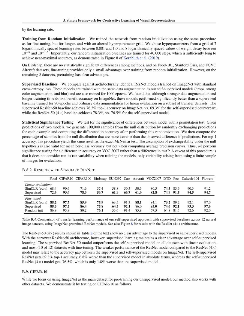
B.8.2. RESULTS WITH STANDARD RESNET
Food CIFAR10 CIFAR100 Birdsnap SUN397 Cars Aircraft VOC2007 DTD Pets Caltech-101 Flowers
Linear evaluation:SimCLR (ours) 68.4 90.6 71.6 37.4 58.8 50.3 50.3 80.5 74.5 83.6 90.3 91.2Supervised 72.3 93.6 78.3 53.7 61.9 66.7 61.0 82.8 74.9 91.5 94.5 94.7
Fine-tuned:SimCLR (ours) 88.2 97.7 85.9 75.9 63.5 91.3 88.1 84.1 73.2 89.2 92.1 97.0Supervised 88.3 97.5 86.4 75.8 64.3 92.1 86.0 85.0 74.6 92.1 93.3 97.6Random init 86.9 95.9 80.2 76.1 53.6 91.4 85.9 67.3 64.8 81.5 72.6 92.0
Table B.4. Comparison of transfer learning performance of our self-supervised approach with supervised baselines across 12 naturalimage datasets, using ImageNet-pretrained ResNet models. See also Figure 8 for results with the ResNet (4×) architecture.
The ResNet-50 (4×) results shown in Table 8 of the text show no clear advantage to the supervised or self-supervised models.With the narrower ResNet-50 architecture, however, supervised learning maintains a clear advantage over self-supervisedlearning. The supervised ResNet-50 model outperforms the self-supervised model on all datasets with linear evaluation,and most (10 of 12) datasets with fine-tuning. The weaker performance of the ResNet model compared to the ResNet (4×)model may relate to the accuracy gap between the supervised and self-supervised models on ImageNet. The self-supervisedResNet gets 69.3% top-1 accuracy, 6.8% worse than the supervised model in absolute terms, whereas the self-supervisedResNet (4×) model gets 76.5%, which is only 1.8% worse than the supervised model.
B.9. CIFAR-10
While we focus on using ImageNet as the main dataset for pre-training our unsupervised model, our method also works withother datasets. We demonstrate it by testing on CIFAR-10 as follows.
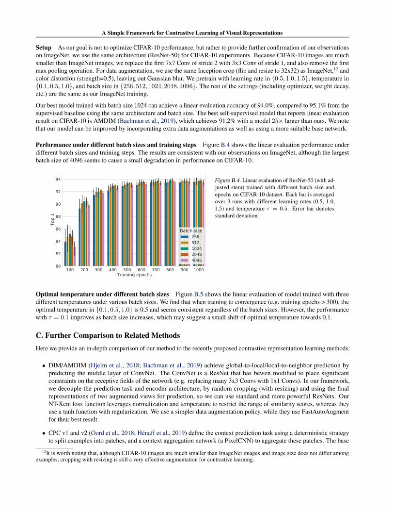
A Simple Framework for Contrastive Learning of Visual Representations
Setup As our goal is not to optimize CIFAR-10 performance, but rather to provide further confirmation of our observationson ImageNet, we use the same architecture (ResNet-50) for CIFAR-10 experiments. Because CIFAR-10 images are muchsmaller than ImageNet images, we replace the first 7x7 Conv of stride 2 with 3x3 Conv of stride 1, and also remove the firstmax pooling operation. For data augmentation, we use the same Inception crop (flip and resize to 32x32) as ImageNet,12 andcolor distortion (strength=0.5), leaving out Gaussian blur. We pretrain with learning rate in {0.5, 1.0, 1.5}, temperature in{0.1, 0.5, 1.0}, and batch size in {256, 512, 1024, 2048, 4096}. The rest of the settings (including optimizer, weight decay,etc.) are the same as our ImageNet training.
Our best model trained with batch size 1024 can achieve a linear evaluation accuracy of 94.0%, compared to 95.1% from thesupervised baseline using the same architecture and batch size. The best self-supervised model that reports linear evaluationresult on CIFAR-10 is AMDIM (Bachman et al., 2019), which achieves 91.2% with a model 25× larger than ours. We notethat our model can be improved by incorporating extra data augmentations as well as using a more suitable base network.
Performance under different batch sizes and training steps Figure B.4 shows the linear evaluation performance underdifferent batch sizes and training steps. The results are consistent with our observations on ImageNet, although the largestbatch size of 4096 seems to cause a small degradation in performance on CIFAR-10.
100 200 300 400 500 600 700 800 900 1000Training epochs
80
82
84
86
88
90
92
94
Top
1
Batch size256512102420484096
Figure B.4. Linear evaluation of ResNet-50 (with ad-justed stem) trained with different batch size andepochs on CIFAR-10 dataset. Each bar is averagedover 3 runs with different learning rates (0.5, 1.0,1.5) and temperature τ = 0.5. Error bar denotesstandard deviation.
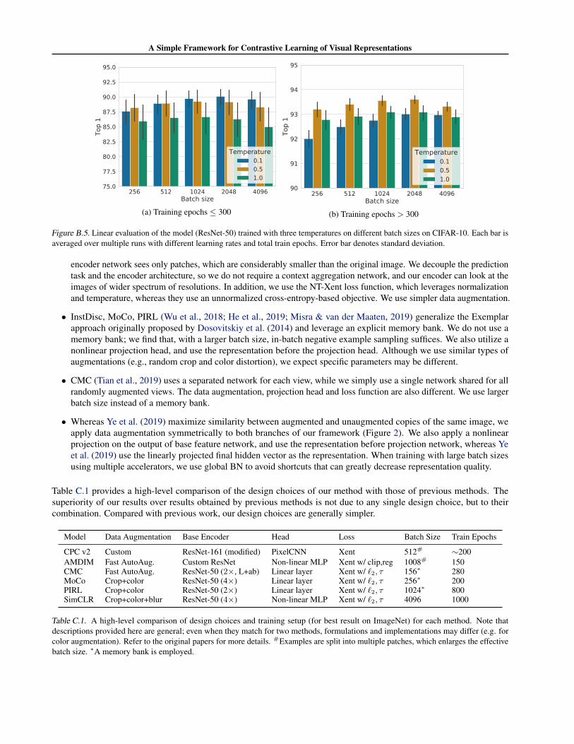
Optimal temperature under different batch sizes Figure B.5 shows the linear evaluation of model trained with threedifferent temperatures under various batch sizes. We find that when training to convergence (e.g. training epochs > 300), theoptimal temperature in {0.1, 0.5, 1.0} is 0.5 and seems consistent regardless of the batch sizes. However, the performancewith τ = 0.1 improves as batch size increases, which may suggest a small shift of optimal temperature towards 0.1.
C. Further Comparison to Related MethodsHere we provide an in-depth comparison of our method to the recently proposed contrastive representation learning methods:
• DIM/AMDIM (Hjelm et al., 2018; Bachman et al., 2019) achieve global-to-local/local-to-neighbor prediction bypredicting the middle layer of ConvNet. The ConvNet is a ResNet that has bewen modified to place significantconstraints on the receptive fields of the network (e.g. replacing many 3x3 Convs with 1x1 Convs). In our framework,we decouple the prediction task and encoder architecture, by random cropping (with resizing) and using the finalrepresentations of two augmented views for prediction, so we can use standard and more powerful ResNets. OurNT-Xent loss function leverages normalization and temperature to restrict the range of similarity scores, whereas theyuse a tanh function with regularization. We use a simpler data augmentation policy, while they use FastAutoAugmentfor their best result.
• CPC v1 and v2 (Oord et al., 2018; Hénaff et al., 2019) define the context prediction task using a deterministic strategyto split examples into patches, and a context aggregation network (a PixelCNN) to aggregate these patches. The base
12It is worth noting that, although CIFAR-10 images are much smaller than ImageNet images and image size does not differ amongexamples, cropping with resizing is still a very effective augmentation for contrastive learning.
A Simple Framework for Contrastive Learning of Visual Representations
256 512 1024 2048 4096Batch size
75.0
77.5
80.0
82.5
85.0
87.5
90.0
92.5
95.0
Top
1
Temperature0.10.51.0
(a) Training epochs ≤ 300
256 512 1024 2048 4096Batch size
90
91
92
93
94
95
Top
1
Temperature0.10.51.0
(b) Training epochs > 300
Figure B.5. Linear evaluation of the model (ResNet-50) trained with three temperatures on different batch sizes on CIFAR-10. Each bar isaveraged over multiple runs with different learning rates and total train epochs. Error bar denotes standard deviation.
encoder network sees only patches, which are considerably smaller than the original image. We decouple the predictiontask and the encoder architecture, so we do not require a context aggregation network, and our encoder can look at theimages of wider spectrum of resolutions. In addition, we use the NT-Xent loss function, which leverages normalizationand temperature, whereas they use an unnormalized cross-entropy-based objective. We use simpler data augmentation.
• InstDisc, MoCo, PIRL (Wu et al., 2018; He et al., 2019; Misra & van der Maaten, 2019) generalize the Exemplarapproach originally proposed by Dosovitskiy et al. (2014) and leverage an explicit memory bank. We do not use amemory bank; we find that, with a larger batch size, in-batch negative example sampling suffices. We also utilize anonlinear projection head, and use the representation before the projection head. Although we use similar types ofaugmentations (e.g., random crop and color distortion), we expect specific parameters may be different.
• CMC (Tian et al., 2019) uses a separated network for each view, while we simply use a single network shared for allrandomly augmented views. The data augmentation, projection head and loss function are also different. We use largerbatch size instead of a memory bank.
• Whereas Ye et al. (2019) maximize similarity between augmented and unaugmented copies of the same image, weapply data augmentation symmetrically to both branches of our framework (Figure 2). We also apply a nonlinearprojection on the output of base feature network, and use the representation before projection network, whereas Yeet al. (2019) use the linearly projected final hidden vector as the representation. When training with large batch sizesusing multiple accelerators, we use global BN to avoid shortcuts that can greatly decrease representation quality.
Table C.1 provides a high-level comparison of the design choices of our method with those of previous methods. Thesuperiority of our results over results obtained by previous methods is not due to any single design choice, but to theircombination. Compared with previous work, our design choices are generally simpler.
Model Data Augmentation Base Encoder Head Loss Batch Size Train Epochs
CPC v2 Custom ResNet-161 (modified) PixelCNN Xent 512# ∼200AMDIM Fast AutoAug. Custom ResNet Non-linear MLP Xent w/ clip,reg 1008# 150CMC Fast AutoAug. ResNet-50 (2×, L+ab) Linear layer Xent w/ `2, τ 156∗ 280MoCo Crop+color ResNet-50 (4×) Linear layer Xent w/ `2, τ 256∗ 200PIRL Crop+color ResNet-50 (2×) Linear layer Xent w/ `2, τ 1024∗ 800SimCLR Crop+color+blur ResNet-50 (4×) Non-linear MLP Xent w/ `2, τ 4096 1000
Table C.1. A high-level comparison of design choices and training setup (for best result on ImageNet) for each method. Note thatdescriptions provided here are general; even when they match for two methods, formulations and implementations may differ (e.g. forcolor augmentation). Refer to the original papers for more details. #Examples are split into multiple patches, which enlarges the effectivebatch size. ∗A memory bank is employed.