A SimMechanics motorcycle tyre model for real time...
96
1 A SimMechanics motorcycle tyre model for real time purposes
Transcript of A SimMechanics motorcycle tyre model for real time...

1
A SimMechanics motorcycle tyre model for real time purposes

2
Summary
Under the name Cruden, headquartered in Oude Meer, is the world's leading interactive
simulation company. Founded in 2004, the company develops, builds, and markets turn
key interactive simulators for the automotive and entertainment industries. With their
simulators they cover broad range car racing.
However a motorcycle simulator would expand their field of activity and for that a
motorcycle tyre model had to be developed. Since the simulator can be driven from any
real time external physics host, the use of SimMechanics was proposed. Which is a
Simulink blockset of Matlab. SimMechanics uses spatial operator algebra to solve the
equations of motion and is ideal for real-time applications, due to the efficiency of the
algorithm. Moreover the method of building the SimMechanics model is easier than
representing the same mechanical system in Simulink. An advantage is the flexibility in
adding components to already created models and to create non-linear systems relatively
easy without deriving the equations of motion. The construction and validation of a tyre
model within this software package is the main subject of this thesis.
The internal force elements of the tyre forces are modelled with impact functions.
Furthermore longitudinal and lateral slip calculations are implemented. After the tyre
model was build and showed satisfying results it build into a bicycle model. The bicycle
model considered here is based on a well-established benchmark model that has been
developed and can be used especially for these kind of validation purposes. Therefore the
dominant dynamics were identified, in the area of interest. All geometric aspects, of the
bicycle model was similar to that used in the benchmark, and differed only in the regions
of the tyres.
As an intermediate step, results are presented of a wheel and a bicycle. Both
characteristics are determined from a stability analysis.
Several experiments with the tyre were conducted. But most of them were not suited to
validate the model because of inadequate simulation set-up or because of noise,
disturbing the signals. The model is optimized by tuning those tyre parameters, which
were estimated in the first place or depend on simulation conditions. Furthermore a first
order filter was implemented in order to improve the tyre behaviour and reduce noise.
The optimized tyre model showed good resemblance at higher speeds. As long as
simulation conditions are within linear range, both model performs reasonable while the
bicycle performs nearly as good as the benchmark.

3
Content
1. INTRODUCTION............................................................................................................................. 5
1.1 PROBLEM DESCRIPTION .......................................................................................................... 5
1.2 MOTORCYCLE DYNAMICS ANALYSIS USING SIMMECHANICS ......................................................... 5
1.3 FURTHER REQUIREMENTS ....................................................................................................... 5
1.4 FUNCTIONALITY OF THE TOOLBOX ........................................................................................... 6
1.4.1 Physical Modeling Blocks .................................................................................................... 6
1.4.2 Visualization tools ................................................................................................................ 7
1.4.3 Mathematical aspects .......................................................................................................... 7
2. ANALYSIS OF THE PROBLEM .................................................................................................... 8
2.1 TYRE MODEL ......................................................................................................................... 8
2.1.1 Tyre description ................................................................................................................... 8
2.1.2 Axis Systems and Definitions W-Axis System .................................................................... 10
2.1.3 Tyre road interaction .......................................................................................................... 10
2.1.4 Construction of wheel element ........................................................................................... 11
2.1.5 Computing road contact point location ............................................................................... 12
2.1.6 Slip Ratios ......................................................................................................................... 15
2.1.7 Force Evaluation ............................................................................................................... 15
2.2 SIMULATION OF THE MODEL................................................................................................... 16
2.2.1 Tyre parameter estimation ................................................................................................. 17
2.2.2 Case 1: non-dimensional experiment dataset ..................................................................... 19
2.2.3 Case 2: bicycle wheel experiment dataset ......................................................................... 20
2.3 DIFFERENCES IN WHEEL VELOCITY ........................................................................................ 22
2.3.1 Defining the contact point velocity ...................................................................................... 23
2.3.2 Defining the contact point velocity based on scalar projections ........................................... 24
2.3.3 First approach of determining the wheel radius derivative .................................................. 25
2.3.4 Defining yaw rate ............................................................................................................... 27
2.4 FINDING THE TIME DERIVATIVE OF THE WHEEL RADIUS VECTOR ................................................. 28
2.4.1 Defining the slip angles ...................................................................................................... 32
2.4.2 Validation of propagation speed ......................................................................................... 32
2.5 TYRE RELAXATION LENGTH ................................................................................................... 33
2.5.1 Turnslip (Pathcurvature) .................................................................................................... 34
2.6 CAMBERTHRUST .................................................................................................................. 35
2.7 ERRATIC SIMULATION DATA ................................................................................................... 36
2.8 THE CRITICAL SPEED OF THE WHEEL ...................................................................................... 36
2.9 STABILITY ANALYSIS ............................................................................................................. 37
2.9.1 Motorcycle wheel experiment dataset ................................................................................ 38
2.10 MOTORCYCLE WHEEL EXPERIMENTS ...................................................................................... 39
2.11 PARAMETER VARIATIONS ...................................................................................................... 46
2.11.1 Different tyre parameters ................................................................................................... 46
2.11.2 Simulation results .............................................................................................................. 47
2.12 CONCLUDING REMARKS ........................................................................................................ 50
2.13 INTEGRATION METHODS ........................................................................................................ 50
2.13.1 Solver type with a fixed time step ....................................................................................... 52
3. SIMMECHANICS JOINT BLOCK MODELING......................................................................... 53
3.1 EULER ANGLES .................................................................................................................... 53
3.2 ANGLE SEQUENCE IN SIMMECHANICS .................................................................................... 54
3.3 PROBLEMS WITH JOINT BLOCK / ERROR TYPE .......................................................................... 56
3.4 BUIDING A MODEL BASED ON THE SIX-DOF JOINT (QUARTERNION) ............................................ 57
3.5 WHEEL COMPARISON BETWEEN CUSTOM AND SIX-DOF JOINT AT 2.5 [M/S] ................................. 58

4
3.6 CONCLUDING REMARKS ........................................................................................................ 58
4. BICYCLE........................................................................................................................................ 59
4.1 INTRODUCTION TO THE BICYCLE MODEL .................................................................................. 59
4.2 CONSTRUCTION OF THE BICYCLE MODEL ................................................................................ 59
4.3 BASIC BICYCLE DESIGN ......................................................................................................... 60
4.4 EIGENVALUE ANALYSIS ......................................................................................................... 61
4.5 BUILDING THE BICYCLE MODEL .............................................................................................. 62
4.6 PROBLEMS WITH THE BICYCLE MODEL .................................................................................... 62
4.7 LATERAL PERTUBATION (CG) ................................................................................................ 63
4.7.1 Bicycle comparison between Custom and Six-DoF joint at 4.292 [m/s] ............................... 64
4.7.2 Bicycle simulations ............................................................................................................ 64
4.7.3 Simulation challenges ........................................................................................................ 66
4.7.4 Steer rate .......................................................................................................................... 67
4.8 DATA ANALYSIS ................................................................................................................... 68
4.8.1 Data Processing ................................................................................................................ 68
4.8.2 Interpolation ...................................................................................................................... 69
4.8.3 Mean zero ......................................................................................................................... 69
4.9 SIMULATION RESULTS........................................................................................................... 72
5. MODEL STRUCTURE AND FEATURES .................................................................................... 74
6. CONCLUSIONS ............................................................................................................................. 76
APPENDICES
APPENDIX A ............................................................................................................. 79
APPENDIX B ............................................................................................................. 80
APPENDIX C .............................................................................................................. 82

5
1. Introduction.
For this assignment we would like to investigate the possibility to design a motorcycle
model in a multibody package.
1.1 Problem description
The aim is to design a simulation model in Matlab/Simulink/SimMechanics. Matlab
scripts will be simulating the driving characteristics of the motorcycle on a racetrack. In
order to get a realistic feeling real motorcycle physics should be implemented. The
simulator should analyze the response to the rider's inputs, torque, brake, and throttle.
Environmental inputs, like road geometry need to be included as well.
1.2 Motorcycle dynamics analysis using SimMechanics
Simulating the dynamics of multibody systems is a common problem in engineering
and science. Motorcycles are complex machines that can exhibit subtle and interesting
nonlinear behaviour. Deriving the governing equations of motion by hand is a tedious
procedure that typically results in errors because of the enormous number of
manipulations necessary. SimMechanics - a toolbox for the Matlab / Simulink
environment - is a numerical program which computes the dynamics on the basis of a
block diagram. Mechanical systems are represented by connected block diagrams. Unlike
normal Simulink-blocks, which represent mathematical operations, or operate on signals.
physical modelling blocks represent physical components, and geometric and kinematic
relationships directly. This is not only more intuitive, it also saves the time and effort to
derive the equations of motion. SimMechanics models, however, can be interfaced
seamlessly with ordinary Simulink block diagrams. This enables the user to design e.g.
the mechanical and the control system in one common environment.
1.3 Further requirements
In the simulator, the rider should experiences the same physical sensations as those
perceived during the driving operation of a real motorcycle. This is valid not only in
terms of visual and the acoustical types of feedback stimuli, but also for perceived sense
of movements, accelerations and decelerations ones, control movements of the vehicle,
and in terms of the physical interactions arising with the real mechanical structure of the
simulator. It is a “motion-based” simulator, i.e. it is equipped with moving parts in order
to reproduce, with some degree of approximation, the dynamics of a real motorbike. The
final system presents the human operator seated on a mock-up of a two-wheeled vehicle.
The mock-up is intended as a rigid structure that is moved with respect to a ground frame
of reference by a mechanism (actuation system) possessing the required number of
degrees of freedom.
The most important features of two-wheeled vehicles are handling, stability and comfort.
They depend on the mechanical characteristics of the vehicle (e.g. steering system
kinematics, mass distribution, tyre properties) but also on the dynamic properties of the

6
bodies of the rider and passenger, because the ratio between the mass of the passengers
and the mass of the vehicle is not as small as in other kinds of vehicles. Hence, the rider
influences the behaviour of the vehicle not only through the voluntary control actions, but
also through the passive behaviour of his/her body, which responds to the motion
imposed by the vehicle.
1.4 Functionality of the Toolbox
This section provides an overview about SimMechanics. The block set is described
briefly, as well as the different analysis modes and visualization options. More details
about these topics can be found in [17].
1.4.1 Physical Modeling Blocks
As already mentioned, the SimMechanics blocks do not directly model mathematical
functions but have a definite physical (here: mechanical) meaning. The block set consists
of block libraries for bodies, joints, sensors and actuators, constraints and drivers, and
force elements. Standard Simulink blocks have distinct input and output ports. The
connections between those blocks are called signal lines, and represent inputs to and
outputs from the mathematical functions. Due to Newton’s third law of action and
reaction, this concept is not sensible for mechanical systems [20]. Special connection
lines, anchored at both ends to a connector port have been introduced with this toolbox.
Unlike signal lines, they cannot be branched, nor can they be connected to standard
blocks. To do the latter, SimMechanics provides Sensor and Actuator blocks. They are
the interface to standard Simulink models. Actuator blocks transform input signals in
motions, forces or torques. Sensor blocks do the opposite; they transform mechanical
variables into signals.
Obviously, every block corresponds to one mechanical component. The properties
of the blocks can be entered by double-clicking on them. These are for example mass
properties, dimensions and orientations for the bodies, the axis of rotation for the
rotational joint and the spring/ damper coefficients for the spring & damper block. The
initial conditions are given directly by specifying the initial position and orientations of
the rigid bodies.
Figure 1: Example of a Pendulum constructed in the SimMechanics body block scheme.
The block diagram solves the problem without the need to derive equations. Let us have a
closer look at the diagram. With this model and the visualization facilities of
SimMechanics it is for example possible to animate the motion of a pendulum. This
pendulum is shown in figure 1. The left block indicated with ‘env’ stands for the
environment, here one can define the gravity, the ground is the origin of the coordinate

7
system, e.g. (0,0,0). The revolute is a one degree of freedom rotational axis. And finally
the body or pendulum is shown.
1.4.2 Visualization tools
SimMechanics offers two ways to visualize and animate machines. One is the build-in
Handle Graphics tool, which uses the standard Handle Graphics facilities known from
Matlab with some special features unique to SimMechanics. The visualization tool can
also be used to animate the motion of the system during simulation. This can be much
more expressive than ordinary plots of motion variables over time. The drawback is a
considerably increased computation time if the animation functionality is used. More
realistic renderings of bodies are possible, with the Matlab Virtual Reality Toolbox.
Arbitrary virtual worlds can be designed with the Virtual Reality Modeling Language
(VRML) and interfaced to the SimMechanics model.
1.4.3 Mathematical aspects
The structure of the equations of motion depends largely on the choice of coordinates.
Many commercial software packages for multibody dynamics use the formulation in
absolute coordinates. In this approach, each body is assigned 6 degrees of freedom first.
Then, depending on the interaction of bodies due to joints, etc. suitable constraint
equations are formed. SimMechanics however, uses relative coordinates [20]. In this
approach, a body is initially given zero degrees of freedom. They are “added” by
connecting joints to the body. Therefore, far fewer configuration variables and constraint
equations are required. Acyclic systems can even be simulated without forming any
constraint equations. The drawback of this approach is the dense mass matrix M, which
now contains the constraints implicitly, and the more complex constraint equations.
Relative coordinate approaches minimize the number of coordinates necessary for
representing the configuration by implicitly parameterize certain constraints (for
example, Joint interactions) between bodies. This re-parameterization is accomplished by
restricting the relative motion between bodies to an allowable subspace. This typically
results in far fewer variables in the configuration vector q and a corresponding reduction
in the number of constraint equations, as compared to the absolute coordinate
formulation. While the dimension of q and the number of constraint equations is
significantly reduced, a drawback with this approach is that the mass matrix M(q) now
becomes dense and the constraint equations more complicated to express. The
computational cost of constructing and inverting the mass matrix contributes significantly
to the overall computational cost of the formulation, and so is an important aspect to
consider.

8
2. Analysis of the problem
In this chapter the problem is analyzed in different steps. The tyre model is explained in
more detail in §2.1. In §2.2 a simulation with the constructed model is performed. §2.3
the wheel velocity is analyzed and §2.4 shows the calculation of the wheel radius vector.
2.1 Tyre model
Already in the early years of vehicle modelling it has been concluded that the behaviour
of a vehicle strongly depends on the tyre behaviour. This holds especially for
motorcycles, as single track vehicles are inherent to instabilities which are partly
governed by the tyre behaviour. Therefore, the quality of a motorcycle model strongly
depends on the accuracy of the tyre model that is implemented. In the following
paragraphs the tyre and its modelling will be explained in relation to the multi-body
package SimMechanics.
2.1.1 Tyre description
In order to describe the behaviour of motorcycle tyres, a tyre model is build. A short
description of the implementation is given below, more information about the model can
be found in paragraph 2.3.4.
An important tool in the description of tyre road contact is the contactpoint.
SimMechanics does not provide a solution for this tyre road intersection in both
coordinate systems (global and local). Therefore an explicit tyre road contactpoint had to
be defined. The main difficulty is that this contact point moves in both coordinate
systems SimMechanics provides. It translates on road surface in the global coordinate
systems. Secondly a material point on the wheel disc has a fixed location vector. This
point will describe a cycloid in the global axis system. A point making contact with a flat
road will have a local position vector that always points vertical from the wheel axis, and
therefore counter rotates in the local wheel disk coordinate system.
Apart from being on the road surface continuously, this point has to be at a distance r
from the wheel center. One has to be careful when taking the vertical distance from the
wheel center to the road surface, due to the fact that in case of wheel camber this distance
isn’t equal to the wheel radius.
First of all the contact routine uses the position and orientation of the wheel and the road
profile to determine the position of the contact point within the definitions we use
[§2.3.5].
Furthermore, the forces and moments are described in both axis systems. Therefore all
forces and moments have a “c” or “w” index, which points out with respect to which
reference axis system they are defined.

9
As described, the contact process between the wheel and road plane there has to be a
point of contact at which the wheel and road plane intersect. This contact calculation,
including ‘collision’ detection and ‘collision’ response, is an important area in simulation
of multi-body systems. However the specific multi-body code SimMechanics does not
support the contact processing.
One approach of contact processing in multi-body mechanical systems is based on the
force and torque model of collision [10, 11]. It is assumed that the contacting bodies
penetrate each other and the separation forces are caused by this penetration. These forces
try to prevent further penetration and to separate the contacting bodies. The tyre
behaviour is implemented by means of a constitutive tyre interface. For the wheel and
wheel plane this means that the wheel penetrates through the road, resulting in a
deformation. This deviation, or in other words, difference between the wheel radius and
defined contact point is a measure for the deformation.
The body sensor assesses the wheel position and orientation. Making it possible to give a
penalty to the wheel. Using a stiffness and damping this is translated into a force which is
applied on the wheel axle with a force actuator.
When modeling a rolling sphere (ball) - as in the SimMechanics rolling sphere example -
denying the contact point to penetrate the road surface, would be exactly equivalent to
constraining the center of mass height. However when allowing a narrow disk to have six
degrees of freedom, it is not possible to constrain the wheel at the height of the center of
mass, since then it wouldn’t be possible to camber the wheel. So instead of this constraint
another approach is used. Therefore an imaginary plane or road is defined. In case there
is no camber angle, the distance from the wheel axle to the contact point should equate
the wheel radius. If not, e.g. the wheel either penetrates through or comes loose from the
road. The contact force magnitude depends on the penetration depth and the penetration
velocity.
Wheel deformation:
cd = ⋅x n (2-1)
Wheel deformation velocity:
sd = ⋅v nɺ (2-2)
The point s denotes the material point on the wheel disc currently in the contact.
Explanation of the difference between ‘c’ and ‘s’ will be given in paragraph 2.4
This deviation is defined as the deformation of the wheel which will be discussed in
paragraph 2.1.5.

10
2.1.2 Axis Systems and Definitions W-Axis System
The coordinate system conforms to the TYDEX conventions described in the TYDEX-
Format [8]. Two TYDEX coordinate systems with ISO orientation are particularly
important, the C- and W-axis systems as detailed in the figure below.
Figure 2: Tydex C- and W-axis systems. Where ‘w’ is the coordinate system at road level
and ‘c’ at the wheel centre.
The C-axis system is fixed to the wheel carrier with the longitudinal x c -axis parallel to
the road and in the wheel plane (x c -z c -plane). The origin O of the C-axis system is the
wheel center. The origin of the W-axis system is the road contact-point (or ‘point of
intersection’) C defined by the intersection of the wheel plane, the plane through the
wheel spindle and the road tangent plane. The orientation of the W-axis system agrees to
ISO. The forces and torques calculated in the tyre model, which depend on the vertical
wheel load Fz along the zw -axis and the slip quantities, are projected in the W-axis
system. The xw – yw - plane is the tangent plane of the road in the contact point C. The
camber angleγ is defined by the inclination angle between the wheel plane and the
normal nr to the road plane (xw – yw -plane).
2.1.3 Tyre road interaction
The tyre-road contact forces are mainly dependent of the tyre mechanical properties
(stiffness and damping), the road condition (the friction coefficient between tyre and road,
the road structure), and the motion of the tyre relative to the road (the amount and
direction of slip). The requirements to transmit forces in the three perpendicular
directions (Fx, Fy en Fz) and to cushion the vehicle against road irregularities involve
secondary factors such as, radial, lateral, and longitudinal distortions and slip. Although
considered as secondary factors, some of the quantities involved have to be treated as
input variables into the system which generate the forces. The illustration below presents
the input and output vectors.

11
Figure 3: Schematic overview of input and output parameters of the tyre model.
In this diagram the tyre is assumed to be uniform and to move over a flat road surface.
The input vector results from motions of the wheel relative to the road. The forces and
moments are considered as output quantities of the tyre model. They are assumed to act
on a rigid disc with inertial properties equal to those of the undeflected tyre.
2.1.4 Construction of wheel element
In order to perform wheel calculations we need to define a wheel plane. Therefore we
need to have knowledge of the wheel position and orientation. Based on these parameters
it is possible to determine positions and orientations. However the body sensor in
SimMechanics only provides this information for the centre of gravity and not for the
contactpoint. Therefore the orientation and contactpoint position have to be constructed
with the aid of vector algebra. Furthermore these vectors in general describe the position
of the wheel center x, the orientation of the wheel axle e0, specified by the Euler angles
and the position of the contact point xc. One wheel element has six positions and six
velocities. Therefore the following states are defined in the SimMechanics model:
The body sensor assesses the wheel position and orientation. The position of the centre of
gravity is given as a three component vector in the global reference system; the
orientations are given by the rotation matrix R(q) as depicted in figure 3. And the angular
velocity is given by an angular velocity vector.
Wheel plane: Road normal example: Surface:
( )c c
g
x
g
y
g
z
∂
∂ ∂
= ∂
∂
∂
x n
0
0
1
c
=
n ( ) 0cg =x

12
Figure 4: Illustration of a 3D wheel element and road surface.
Initial condition of the wheel axle:
( )*
0 0 1 0T
e = − (2-3)
2.1.5 Computing road contact point location
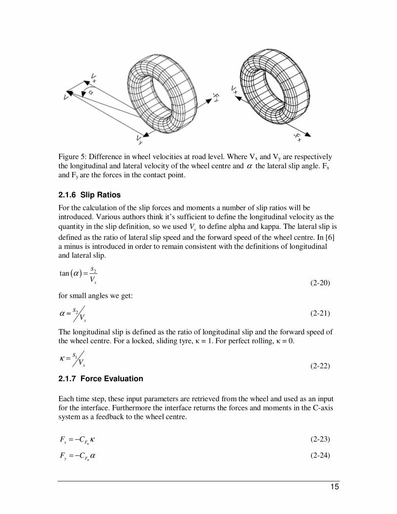
With these states and initial assumptions it is possible to derive an expression for the wheel radius vector and therefore the contact point position.
Rotation matrices are used to transform the components of any vector from one
coordinate system representation to another, rotated coordinate system representation. The rotation matrix R describes the rotational motion of the body in terms of rotation of
the centre of gravity coordinate system axes with respect to the World axes. The product of the rotation matrix and initial wheel axle vector results in the rotated wheel axle:
( ) *
0 0R q=e e (2-4)
By taking the cross product of the rotated wheel axle and road normal one gets the longitudinal vector:
0= ×l n e (2-5)
To form a vector base, the vectors should be orthonormal: orthogonal and unit length. In Matlab/SimMechanics the vectors are not represented with unit length. Therefore the
longitudinal vector has to be normalized to obtain a contact point vector basis.
13
long =l
el
(2-6)
For the lateral direction one follows the same reasoning as for the longitudinal vector.
Using the cross product of the road normal and normalized longitudinal vector results in
the lateral direction. The angle between longitudinal and normal is 90° and thus the
result of their cross product is automatically unit length.
lateral long= ×e n e (2-7)
In order to calculate the wheel radial direction, the cross product of the longitudinal and current wheel axle vector is used. Again automatically becoming unit length.
0r long= ×e e e (2-8)
The wheel radial direction times the length scalar value yields the radius vector:
rr= ⋅r e (2-9)
Where r is the position vector drawn from wheel centre. And r is its linear distance from
the wheel centre to the point of contact.
As explained earlier the rotation matrix is used to describe the rotational motion of the wheel axes with respect to the world axes.
( ) *
0 0R=e p e (2-10)
The equations allow us to locate the theoretical contact point between the tyre and the road, for every wheel attitude. And it travels along the path of the wheel. By summing the
wheel axle position and wheel radius vector:
c rr= + ⋅x x e (2-11)
For the construction of the wheel vectors [6] uses a scaling factorλ . This rescaling is
necessary in case the road normal and rotated wheel axle aren’t perpendicular i.e. the camberangle is non zero. Even when both vectors have length 1. So when creating a
longitudinal vector having length 1, means you have to rescale ( )cos γ .
Substitution of equation (2-9) into (2-11)
c = +x x r (2-12)

14
Contact point deformation or penetration depth. Assuming that the road surface is a plane through (0,0,0), we could write:
( )d = + ⋅x r n (2-13)
Contact point deformation or penetration velocity:
( )( )d
ddt
= + ⋅x r nɺ (2-14)
The angular velocity vectorω is the rate at which a spinning coordinate system rotates.
The velocity is tangential to the circular path, i.e. perpendicular to position vector. Using
the velocity of the wheel axle and the wheel rotation speed it is possible to determine the velocity of the material point in the contact.
s = + ×V x ω rɺ (2-15)
The subscript s denotes the location on the wheel plane material point.
To get the slip in longitudinal direction the velocity has to be projected on the longitudinal vector:
1 long sxs = ⋅e V (2-16)
The lateral slip can be obtained in the same way as the longitudinal slip. Hence the
velocity has to be projected on the lateral vector:
2 lat sys = ⋅e V (2-17)
x longV = ⋅e V (2-18)
Where V is the three dimensional centre of gravity velocity vector.
x
y
z
= =
V x
ɺ
ɺ ɺ
ɺ
(2-19)
In this origin the input variables any tyre model e.g. the ‘Magic Formula’, the vertical load Fzw, the longitudinal slip kappa, the side slip angle alpha and the camber or
inclination angle gamma are determined by this routine.
15
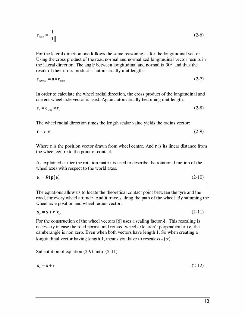
Figure 5: Difference in wheel velocities at road level. Where Vx and Vy are respectively
the longitudinal and lateral velocity of the wheel centre and α the lateral slip angle. Fx
and Fy are the forces in the contact point.
2.1.6 Slip Ratios
For the calculation of the slip forces and moments a number of slip ratios will be
introduced. Various authors think it’s sufficient to define the longitudinal velocity as the
quantity in the slip definition, so we used xV to define alpha and kappa. The lateral slip is
defined as the ratio of lateral slip speed and the forward speed of the wheel centre. In [6]
a minus is introduced in order to remain consistent with the definitions of longitudinal and lateral slip.
( ) 2tanx
s
Vα =
(2-20)
for small angles we get:
2
x
sV
α ≈
(2-21)
The longitudinal slip is defined as the ratio of longitudinal slip and the forward speed of the wheel centre. For a locked, sliding tyre, κ = 1. For perfect rolling, κ = 0.
1
x
sV
κ = (2-22)
2.1.7 Force Evaluation
Each time step, these input parameters are retrieved from the wheel and used as an input
for the interface. Furthermore the interface returns the forces and moments in the C-axis system as a feedback to the wheel centre.
x FF C= −
κκ (2-23)
y FF C= −
αα (2-24)

16
The normal force Fz is calculated assuming a linear spring (stiffness: k) and damper
(damping constant c), so the next equation holds:
zF k d cd= + ɺ
(2-25)
The normal compression d of the tyre on the road can be defined by the tyre free radius
Where d is the deflection and dɺ the deflection velocity.
If the tyre loses contact with the road, the tyre deflection and deflection velocity
become zero, as a consequence the resulting normal force Fz will be negative.
2.2 Simulation of the model
For building a SimMechanics model, the same basic procedure can be used as those for
building a regular Simulink model. From the SimMechanics library, the blocks needed to represent the model can be dragged and dropped into a Simulink model window. When
creating a model one first starts by selecting a ‘environment’ followed by the ‘ground’. Next a joint and body can be selected, The essential result of this step is creation of a
valid tree block diagram made of:
Ground -- Joint -- Body -- Joint -- Body -- ... – Body
In which the different names represent:
• Ground: o blocks represent immobile ground points at rest in absolute (inertial) space.
• Joint: o blocks represent relative motions between the Body blocks to which they
are connected.
• Body: o blocks represent rigid bodies.
With the above mentioned formulas the wheel model is build in SimMechanics as shown in Figure 5. Based on the bicycle this process is explained in more detail in APPENDIX C

17
Figure 6: SimMechanics block diagram representation for the wheel model.
The model is build with respect to an right handed orthogonal axis system (O,x,y,z). The origin O of this axis system lies in the contact point between the tyre and the ground
plane. The gravity g is pointing in the –z direction. The body model is composed of one rigid part.
In this study the first aim was to look at rolling motion with a small yaw velocity
behaviour and investigate the stability. The aim was to have the wheel follow a reference profile for the roll angle.
2.2.1 Tyre parameter estimation
A method for developing a tyre model is to imagine the tyre as a one degree of freedom mass-spring system. Mathematically this is defined as
0mx cx kx+ + =ɺɺ ɺ (2-26)
with damping (c) and stiffness (k)
The damping ratio is defined as.
2
c
kmζ = (2-27)
The eigenfrequency is defined as
nk
mω = (2-28)
Substitution of equation (2-28) into (2-27) yields
2 n
c
mζ
ω= (2-29)

18
The longitudinal ( )xF and lateral ( )yF force are defined as
xx F
x
sF C
V= −
κ (2-30)
y
y F
x
sF C
V= −
α (2-31)
To find out the wheel behaviour the wheel has to be validated. For this purpose we would
like to use the disk described by Schwab in his dissertation [24]. The discrepancy is that
the disk described in [24] is rolling without slip over a horizontal plane. However it is
assumed for both models that this is a infinitesimally thin disk and has an uniformly
distributed mass m, unit radius r, and a gravitational force field g in the downward
direction. Since our wheel is constructed with slip and deformation/penetration through
the road. This would not be a 100% correct validation. A way to approximate this
kinematic/rigid rolling is to increase the parameters of the tyre to infinity. This procedure
is explained in more detail in the next paragraph. The problem that occurs is that the step
size in the solver has to be very close to zero. Hence smaller time steps results in a higher
accuracy. Resulting in a enormous simulation time or errors. So if we want to find out the
critical velocity of the wheel where it shows an undamped oscillatory behaviour there
would be a significant difference in output behaviour compared to the kinematic rolling
disk.
Another way to validate the wheel model, is with the use of the available linearization
tool (linmod) in Matlab. That makes it possible to linearise the system and check whether
the system is stable, based on a root loci plot. However one of the requirements of this
tool is that the system to be investigated is in equilibrium. Since the wheel can be
imagined as an inverted pendulum, this is not the case. A different approach by hanging
the wheel to the road would not be an option since you would like to act the gravitational
force as an force pointing downwards. Another problem is that the model is complicated
due to al the output en input needed for the calculation of the forces and moments. For
that reason we wanted to analyse the model based on a time domain simulation. So based
on the time period of the oscillation, the frequency is determined. By increasing the
wheel parameters (stiffnesses) we can verify if the system can be matched (shows the
same behaviour) with the rigid rolling disk of [24].
Since only a few eigenfrequencies could be found with the standard linmod tool (an
command in Matlab to linearize a model) and due to the complex behaviour of the wheel,
the linmod tool could not give the desired information. For that reason we decided to
analyze the linearization behaviour based on a convergence plot. (Against a characteristic
value) So by increasing the parameters with a factor and by calculating the difference in
eigenfrequency, we are able to see if the eigenfrequency is converging. To do so, the
eigenfrequency has to be calculated at every oscillation. With the aid of the fit function
tool in Matlab we are able to calculate the time period at which the wheel is oscillating.
Based on the time period we can calculate the eigenfrequency.

19
Wheel parameters:
• Vertical tyre stiffness: k
• Damping: c
• Longitudinal tyre stiffness: F
Cκ
• Lateral tyre stiffness: F
Cα
Characteristic value:
1n n
n abs
f f
f
Characteristic value
Characteristic value
ω ω
ω
−= −
=
2.2.2 Case 1: non-dimensional experiment dataset
One of the purposes of this research is to investigate the behaviour of the tyre model.
Therefore, several simulations are conducted at different tyre parameters. In this section
the results of a simulation with a forward velocity of 1 [m/s] are presented. We will
assume that the infinitesimally thin wheel has uniformly distributed unit mass, unit radius
r and a unit gravitational force field g in the downward direction.
• Inertia matrix:
0.25 0 0
0 0.5 0
0 0 0.25
Assuming a damping ratio in the order of 25%, a maximum slip force of m*g [N], and a
forward velocity of 1 [m/s]. Allowing a slip, max max,α κ of 1/1000 results in a slip stiffness
in the longitudinal and lateral direction in the order of 1000.
max
1F
C =κκ
(2-32)
max
1F
C =αα
(2-33)
Based on the above expressions and for convenience, we take for the disk parameters.
• Vertical tyre stiffness k=1000[N/m]
• Damping c=20 [Ns/m]
• Longitudinal tyre stiffness F
Cκ=1000 [N]
• Lateral tyre stiffness F
Cα
=1000 [N]

20
Simulation results
If only the qualitative motion of a mechanism is of interest, the animation facilities of
SimMechanics come into play. Figure 7 shows an example of the automatically generated
animation window.
Figure 7: Wheel rolling on a horizontal plane. This is a standard visualization tool in
SimMechanics.
Figure 8: Slip as a function time of respectively the lateral, left figure and longitudinal
direction, right figure.
Although the visualization of the wheel motion seemed normal, the measured slip angles
in longitudinal but mainly in lateral direction showed numerical instabilities, as can been
seen in Figure 8. Therefore another experiment was performed with a new set of
parameters.
2.2.3 Case 2: bicycle wheel experiment dataset
For this second experiment the tyre parameters are tuned is such a way that the tyre size
and weight matches a bicycle wheel.
• Mass: 1.65 [kg]
• Wheel radius: 26 [inch]
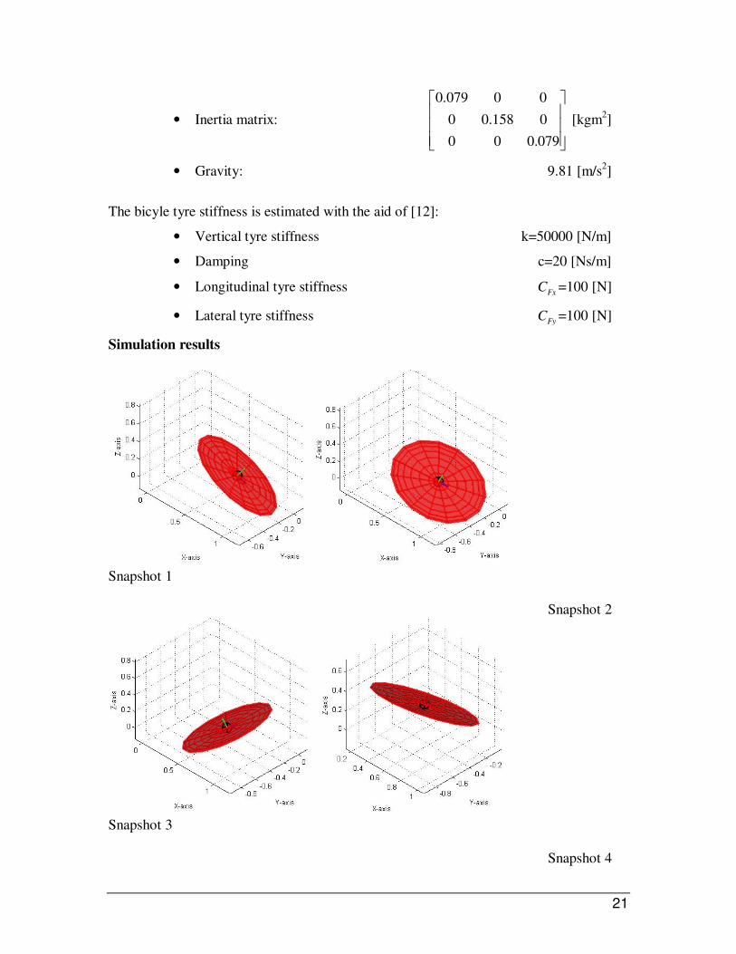
21
• Inertia matrix:
0.079 0 0
0 0.158 0
0 0 0.079
[kgm2]
• Gravity: 9.81 [m/s2]
The bicyle tyre stiffness is estimated with the aid of [12]:
• Vertical tyre stiffness k=50000 [N/m]
• Damping c=20 [Ns/m]
• Longitudinal tyre stiffness Fx
C =100 [N]
• Lateral tyre stiffness Fy
C =100 [N]
Simulation results
Snapshot 1
Snapshot 2
Snapshot 3
Snapshot 4

22
Figure 9: Snapshots of the wheel on a horizontal plane (wobble). With a initial forward
velocity of 0.62 [m/s]. The wheel centre is almost standing still while the contact point is
moving fast.
This simulation showed a wobbling behaviour with decreasing velocity, the simulation
tended to crash, due to the time steps taken for the simulation were getting to small,
making the simulation time growing to infinity. As can be seen in Figure 9, where peaks
are visible around 8.5 seconds.
Figure 10: Slip as a function time of respectively the lateral, left figure and longitudinal
direction, right figure.
It seemed that the problem could be found in the division in the definition of the slips.
The amount of slip is calculated with the aid of the wheel axle speed (wheel centre).
During the wobbling motion the wheel centre speed can physically become zero. As a
consequence the slip ration calculation tends to dividing by zero, which periodically
makes the numerical integration very (infinite) stiff. That is why simulation data shows
numerical instabilities. In literature [6] distinction is made between the wheel axle ( )xV
and the contact point speed. These differences are described in the next paragraph.
2.3 Differences in Wheel velocity
In case a wheel is rolling over a flat road, showing no camber angle or yaw rate ( 0)γψ =ɺ ,
both velocities are equal r x
V V= . Where r
V is defined as the velocity with which an
imaginary point that is positioned on the line along the radius vector r and coincides with
point S at the instant of observation, moves forwards (in x direction) with respect to point
S that is fixed to the wheel rim.

23
Figure 11 Rolling and slipping of a tyre over an undulated road surface. Where ‘s’ is the
material contact point. And Vx and Vcx are respectively the wheel center speed and
propagation speed.
For a better understanding of the above figure a few formulas are denoted. c
= +V V rɺ
Where C is the speed of the propagation represented by c
V . The velocity vector of point
S that is fixed to the wheel body results from s
= + ×V V ω r where ω is the angular
velocity of the wheel body with respect to the inertial frame.
cx c long= ⋅V V e (2-34)
sx s long= ⋅V V e (2-35)
Where the long
e is defined as the longitudinal vector.
r cx sx= −V V V (2-36)
Pure rolling can even occur for a cambered wheel showing yaw rateψɺ and the wheel
center 0x
V = . In that case a linear speed of rolling arises that is equal to
( )sinr
V r γ ψ= ɺ and consequently an angular speed of rolling ( )sinr
ψ γΩ = ɺ .
Furthermore in [6] distinction is made between r ande
r . Where r is defined as the loaded
radius and e
r as the effective rolling radius. Since the difference between both radiuses is
very small and we restrict our self to the physical radius at road level, this variable is not
taken into account. In practice both radius’s lie close together, therefore we assume they
are equal.
2.3.1 Defining the contact point velocity
In stead of the using the wheel center speed we would like to use the propagation speed.
For this reason the calculation of the propagation has to be calculated and the slip angles
have to be redefined. The propagation velocityc
V is constructed out of two velocity
vectors. for the description of the contact speed Pacejka introduces in [6] the wheel radius

24
derivative: c
= +V V rɺ . Respectively the of the wheel center A by b+a. The orientation of
the wheel spin axis is given by unit vector s and the location of the contact center by
x.c
= +V V rɺ . The SimMechanics body sensor gives the wheel centre velocity, so we have
to calculate the contribution of rɺ .
Figure 12: Definition of position, attitude and motion of the wheel and the forces and
moments acting from the road on the wheel [6].
2.3.2 Defining the contact point velocity based on scalar projections
Since r formally is a result of two cross products as described in (2-8), it is not easy to
determine the derivative of this vector. Another way of describing this velocity is with
the aid of scalar projections. Although it is hard to get an intuitive feel how all the various
vectors are acting. For a better understanding of the above mentioned projections, a
sketch is drawn.
25
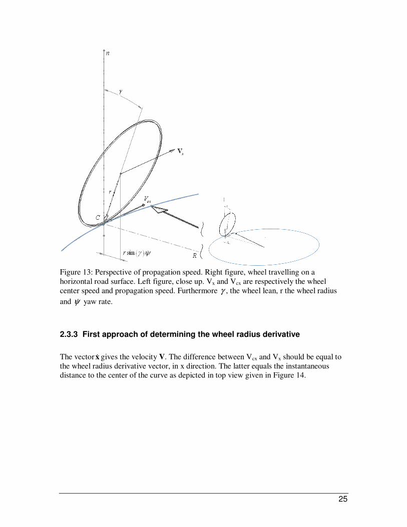
Figure 13: Perspective of propagation speed. Right figure, wheel travelling on a
horizontal road surface. Left figure, close up. Vx and Vcx are respectively the wheel
center speed and propagation speed. Furthermore γ , the wheel lean, r the wheel radius
and ψɺ yaw rate.
2.3.3 First approach of determining the wheel radius derivative
The vector xɺ gives the velocity V. The difference between Vcx and Vx should be equal to
the wheel radius derivative vector, in x direction. The latter equals the instantaneous
distance to the center of the curve as depicted in top view given in Figure 14.

26
Figure 14: Sketch of wheel radius derivative top view. Where rɺ is the wheel radius
derivative γ , the wheel lean, r the wheel radius and ψɺ yaw rate.
The vector is projected onto the road surface with ( )sinr γ . A closer look learns that this
radius rotates with a velocity equal to the yaw rate. Two parameters which are already
known are the wheel radius r and ( )sin γ . The wheel camber or wheel inclination angle
( )γ is defined as the angle between the wheel-centre-plane and the normal to the road.
( ) 0sin γ = ⋅n e (2-37)
Which results in the road surface projection of the wheel radius vector. For determining
the contribution of ( )sin γ , this expression needs to be multiplied with the wheel radius.
After this multiplication the vector has a scalar distance,
The next component in the calculation is momentarily rotational velocity or yaw rate. The
angular velocity vector ω can be obtained using the SimMechanics body sensor block.
Since we are interested in the yaw rate it seems legitimate to take the third or better
normal- component of the wheel body rotational velocity:
ψ = ⋅n ωɺ . (2-38)

27
Derivative of wheel radius vector: cxr sxV V V= − or
cx xV V− = ( ) [ ]( )0sin lat longr r= ⋅ ⋅n e e eɺ ɺψ γ ψ (2-39)
Wheel contact point velocity
c x= +V V rɺ (2-40)
( )sincx x
V V r γ ψ= + ɺ (2-41)
After summing the velocities, projection of the contact point velocity on the longitudinal
direction gives .
cx c longV = ⋅V e (2-42)
Although this gave better results, the formulation is not correct. The calculation of rɺ leads
to nois in the determination of α and κ as well. The problem lies in the yaw rate
definition which is described in the next paragraph.
2.3.4 Defining yaw rate
As explained in the previous paragraph, in the definition of the yaw rate one has to be
careful. Hence ψɺ may not be confused with the projection of the third component of ω ,
due to a contributing effect of rolling Ω in the z component ofω . For example when a
wheel is rolling straight and upright the third component of ω is zero. i.e. the trajectory is
straight and the yaw rate is zero. In a similar situation, again rolling along a straight line,
but with a cambered wheel, with no steer input or yaw rate. The third component of
omega is equal the ( )sin γΩ . Hence an increasing camber angle results in a contributing
effect on the projection in the third component of the wheel rotation. But obviously a
straight path does not experience yaw rate. Therefore we have to look at the rotation
which does not coincide with the spinning axis. For an accurate representation of the
direction of travel, this rotation has to be projected onto the road normal.
According to [6], the yaw rate is defined as the speed of rotation of the line of
intersection about the z axis normal to the road. In vector notation:
long lat= ⋅ψ e eɺ ɺ (2-43)
For this we need the time derivative of the longitudinal vector. Which will be derived in
the next paragraph as an intermediate result. We need to conclude here that the physical
interpretation of the contact point propagation speed will hardly be beneficial for
avoiding vector algebra.

28
2.4 Finding the time derivative of the wheel radius vector
In the previous paragraphs we tried to get a correct formulation of the propagation speed,
based on scalar projections. The wheel radius vector derivative rɺ is not a straight forward
calculation. [6] does not indicate that the derivative of the wheel radius vector is a result
of three successive rotations, and scaling effects. Furthermore this scaling effect has to be
included in the derivation as well. Several steps are taken to get to the solution. We
already defined:
( )0longr= ×r e e (2-44)
( )0 0long longr= × + ×r e e e eɺ ɺ ɺ (2-45)
Or
0 0r long long= × + ×e e e e eɺ ɺ ɺ (2-46)
From equation (2-46) it can be seen that for the calculation of the wheel radius derivative
the derivative of the longitudinal vector is needed. This vector is the result of a cross
product itself, but it is important to notice that this vector has to be normalized to give the
vector unit length. Therefore the numerator shows a time dependent term, as the angle
between the road normal and wheel plane(=camber) can vary.
long=
le
l (2-6)
Knowing that the length of 0e and n both are equal to one, we can write sin=l θ
sinlong
=l
eθ
(2-47)
In case the angle θ between the vectors of the road normal vector and wheel axle is
smaller than 90 degrees. i.e. a decrease of the parallelepiped with adjacent sides 0e and n ,
results in a scaling of long
e . This effect has to be compensated in the derivative of the
wheel radius vector. Moreover the sinθ term in the numerator of the longitudinal vector
is time dependant and therefore it must be taken into account.

29
Figure 15: Schematic overview of the contributing effect of θ , due to time dependency
of the longitudinal vector long
e . Which is calculated with the cross product of the rotated
wheel axle and road normal.
With the relation stated in (2-45) the derivative of equation (2-8) can be written as:
0 0sin sin
r
d
dt
= × + ×
l le e eɺ ɺ
θ θ (2-48)
Recalling the quotient rule for derivation of the first term,
2
sin cos
sin sinlong
de
dt
− = =
l l l ɺɺɺ
θ θθ
θ θ (2-49)
The derivative of the longitudinal vector l
0 0= × + ×l n e n eɺ ɺ ɺ (2-50)
However as stated before the scaling should be taken into account
2
sin coscot
sin sinlong long
−= = −
l l le e
ɺɺ ɺɺɺ
θ θθθθ
θ θ
(2-51)
In de expression (2-50), that will be substituted in (2-49), 0
eɺ is required; the time
derivative of the rotated wheel axle. It can be found in the following quite formal way:
** 0
0 0
dR dR
dt dt= +
ee eɺ (2-52)
With the orthogonallity property of the rotation tensor T
RR I= the expression can be
rewritten as. *
0 0
TdRR R
dt=e eɺ the last part ( ) *
0R p e is equal to 0e .
The relation between the time derivatives of the rotational parameters and the angular
velocity is known as the Poisson equation. The relation 0×ω e indicates that the action
×ω is equivalent to T
RRɺ indicating that T
RRɺ is an skew-symmetric tensor.
longe
0e
n
θ
30
0 0
TdRR
dt=e eɺ (2-53)
TRR× =ω ɺ (2-54)
Substitution of (2-53) and (2-54) into (2-52) yields which could be anticipated but is now
proven in a more formal framework.
0 0= ×e ω eɺ (2-55)
This result leads to the following lɺ :
( )0 0= × + × ×l n e n ω eɺ ɺ
(2-56)
For the second term in equation (2-56) we can use the vector ‘triple product’:
( ) ( ) ( )× × = ⋅ − ⋅a b c b a c c a b (2-57)
That transforms (2-56) into:
( ) ( )0 0 0= × + ⋅ − ⋅l n e ω n e e n ωɺ ɺ (2-58)
And finally lɺsubstituted in (2-49) leads to:
( ) ( )( )0 0 0
2
sin cos
sinlong
× + ⋅ − ⋅ −=
n e ω n e e n ω le
ɺɺɺ
θ θθ
θ (2-59)
Or:
( ) ( )( )0 0 0cot
sinlong long
× + ⋅ − ⋅= −
n e ω n e e n ωe e
ɺɺɺ θθ
θ (2-60)
Now 0eɺ found from (2-55) can be substituted in (2-48)
( )0 0r long long= × + × ×e e e e ω eɺ ɺ (2-61)
Substitute (2-59) in the above
( ) ( )( )( )0 0 0
0 02
sin cos
sin sinr × + ⋅ − ⋅ −
= × + × ×
n e ω n e e n ω l lr e ω e
ɺɺɺ
θ θθ
θ θ (2-62)
Using the general relation (2-49) for the last term in equation (2-58)
( ) ( )( )0 0 0
0 0 02
sin cos
sin sin sinr × + ⋅ − ⋅ −
= × + ⋅ − ⋅
n e ω n e e n ω l l lr e ω e e ω
ɺɺɺ
θ θθ
θ θ θ (2-63)
31
Since we are interested in the propagation speed, which has its contribution in the
longitudinal direction, the derivative of the wheel radius vector has to be projected onto
the longitudinal vector.
( ) ( )
21
430 0 0
0 0 02
sin cos
sin sin sinlong longr
× + ⋅ − ⋅ − ⋅ = × + ⋅ − ⋅ ⋅
n e ω n e e n ω l
l lr e e ω e e ω e
ɺɺ
ɺ
θ θθ
θ θ θ(2-64)
In order to simplify the above equation we can use some vector relations and general
properties. The derivative of n on flat level roads is zero. ( ) 0c
d
dt=n erasing 0×n eɺ
See 1 in
(2-64)
The cross product of a vector with itself is zero.
0 00×e e ≜ (2-65)
Therefore we lose 2
As the cosine of 90° is zero, the dot product of two orthogonal vectors is always zero.
* 0 0l
⋅e e ≜ (2-66)
Which allows to erase 3 and
4 Therefore we can write.
( )0
02
sin cos
sinlong long
r ⋅ −
⋅ = × ⋅
ω n e lr e e e
ɺɺ
θ θθ
θ (2-67)
A further simplification is obtained with the last term, being projected on the longitudinal
direction vector:
( )( )0
0 0cotsin
long long long longr ⋅
⋅ = × ⋅ − × ⋅
ω n er e e e e e eɺɺ θθ
θ
(2-68)
In the second term the cross product can be identified as the definition of the radial
direction vector (2-8). This yields:
( )0
0 cotsin
long long r longr ⋅
⋅ = × ⋅ − ⋅
ω n er e e e e eɺɺ θθ
θ
(2-69)
Now the second term in
(2-69)
disappears since the dot product of two orthogonal vectors equals zero.
Clearly, scaling a velocity vector means manipulating the length of this vector. In (2-64)
we can see the projection of the two orthogonal vectors, therefore we conclude that in
longitudinal direction there is no velocity contribution due to ignoring or introducing the
time derivative of the scalingθɺ . Indeed there is a projection on rɺ but this is acting in

32
radial direction and known as the penetration velocity. However we already defined the
penetration velocity (2-14) direction, therefore we may ignore its contribution.
2.4.1 Defining the slip angles
In the previous paragraph rɺ is determined. Now we are able to redefine and calculate the
slip angles.
Figure 16:
The lateral slip is defined as the ratio of lateral slip and the forward velocity of the tyre
contact point.
( )2
cx
S
Vα
ε=
+ (2-70)
The longitudinal slip is defined as the ratio of longitudinal slip and the forward velocity
of the tyre contact point.
( )1
cx
S
Vκ
ε=
+ (2-71)
Additional to the earlier stated speeds we now have the extra contribution of the
propagation. Finally we have to be robust in our definition, for example when wheel lock
occurs or in case the angular velocity of the wheel changes sign. For these situations we
introduce a small factor epsilon and make the velocity absolute.
2.4.2 Validation of propagation speed
With the redefined slip angles, the SimMechanics model of the second experiment is
adjusted. We can perform an experiment to validate the correctness. Based on the same
parameters and initial conditions as the bicycle wheel experiment in paragraph 2.2.3. As
can be seen in Figure 17, the wheel falls into an almost cyclic motion during the first turn.
In this motion the centre of mass mainly moves in the downward direction while the
rotation of the point of contact increases rapidly. The disk eventually will come to the
singular horizontal rest position in a finite time. This behaviour can be compared with
the “Euler’s disk”; a smooth edged disk on a slight concave supporting bowl which
whirrs and shudders to a horizontal rest [26].

33
The centre of mass in Figure 17 shows that the simulation keeps on going even if the
wheel centre reaches zero velocity. The contactpoint on the other hand show the rapid
changes in velocity.
Figure 17: Velocity as function of time. Simulated with a initial forward velocity of 0.62
[m/s] centre of mass and contact point respectively.
Figure 18: Slip as a function time of respectively the lateral, left figure and longitudinal
direction, right figure.
2.5 Tyre relaxation length
Simulation of the model showed numerical instabilities. In order to reduce this amount of
noise on the lateral and longitudinal input forces, we build in a first order filter. However
a physical correct representation of this filter can act like a tyre relaxation length.
Furthermore a relaxation length gives more or less a damper in series, which is
representing the behaviour of friction.
1Filtered
s
αα
τ=
+ (2-72)
Where τ is defined as a time constant which is determined by y
cxV
σ. In which
yσ is a
constant.

34
y
F F
cxV
σα α α= −ɺ (2-73)
1
F
y
cx
sV
αα
σ=
+
(2-74)
Where the lateral slip angle equals:
2
cx
s
Vα = (2-75)
Substitution of equation (2-75) into (2-74) yields.
2
y
F cx F
cx
s VV
σα α= −ɺ (2-76)
Rearranging and integration of equation (2-76) results in the filtered lateral slip angel.
2 cx FF
y
s V αα
σ
−= ∫ (2-77)
The same holds for the longitudinal slip:
1 cx FF
x
s V κκ
σ
−= ∫ (2-78)
This is considered to be a more physically accurate representation. At this stage of
modelling a constant relaxation length for the tyre is employed.
2.5.1 Turnslip (Pathcurvature)
The turnslip or pathcurvatureϕ is defined as change of heading direction normalized by
the speed:
V
ψϕ =
ɺ (2-79)
This equals the path curvature of a piece of trajectory. Literature shows that this is a good
measure for calculating the friction resistance moment around the normal axis, so using
(2-76) like in the previous longitudinal and lateral slip calculations, could result in a
devision by zero. To overcome this problem we can apply a spring in series with the
damper. This results in a physical interpretation of a first order filter like earlier stated.
1Filtered
s
ψψ
τ=
+ (2-80)

35
Where τ is defined as a time constant which is determined by cx
Vϕσ
. In which ϕσ is a
constant.
F F
cxV
ϕσψ ψ ψ= − (2-81)
1F
cx
sV
ϕ
ψψ
σ=
+
(2-82)
Where ϕ is defined as:
*t
cxV
ψϕ =
ɺ(see also [6] equation (2-18)) (2-83)
Where: ψ = ⋅n ωɺ
Substitution of equation (2-83) into (2-82) yields.
F t cx F
cx
VV
ϕσψ ϕ ψ= −ɺ
(2-84)
Rearranging and integration of equation
(2-84) results in the filtered turn slip.
t cx FF
V
ϕ
ϕ ψψ
σ
−= ∫ (2-85)
2.6 Camberthrust
The tyre side forces depend on the slip and camber angle and on the tyre vertical load.
Furthermore it has been concluded that for motorcycle tyres, sideslip angles are small and
cornering is mainly possible by camber thrust [6].
In order not to fall over, there is a relation between the side force and normal force with
respect to lean angle. ( )tanyF m g γ= . In which γ is the lean angle. So this amount of side
force (Fy), at a certain lean angle is always present. However there is always the desire to
build up this side force with camber as well. What we therefore would like to do is to
follow this line. Furthermore due to the laws of friction the tyre is limited.
w nF F µ=
(2-86)
There are several cases where ( )tan γ µ> . For example it is very likely that if the bike
lean angle is larger than 45 degrees, the ( )tan 1γ = . i.e. one arrives at the maximum of
what is possible. So a larger lean angle is only possible if the value of µ is increased. This
is only the case if the tyre delivers this shortness. Which means that till 45 degrees is

36
covered with camber and an increasing lean angle has to be compensated for with µ .In
reality however this is much more smooth. A few possibilities are:
y nF Fγ
γ=
(2-87)
( )siny nF Fγ
γ=
(2-88)
( )1 sin 22y nF F
γγ=
(2-89)
The linearized behaviour of all these camber thrust proposals is y n
F F γ= , therefore the
camberthrust provides the lateral force needed in stationairy equilibrium for small camber
angles. All suggested camber forces provide less than the required ( )tany nF F γ= . The
missing side force will then be generated by sideslipα .
2.7 Erratic simulation data
In a multi-body modeling environment the tyre can be considered as a force element. In
the direction normal to the road the tyre behaves as a spring/damper. And for motions
perpendicular to the road plane the tyre develops reaction forces as a result of the relative
(sliding) motion with respect to the road surface.
Due to the erratic results of our constructed tyre model we proposed to compare the
behaviour with another tyre model located in the demo toolbox of SimMechanics. The
constructed model is build with the aid of vector algebra. The example model, located in
the Matlab library, however uses global coordinates. This is one of the main differences.
Furthermore the example model consists of a full non linear motorcycle model, based on
the Autosim code [2]. Since we are only interested in the tyre model, the motorcycle
model had to be disassembled and adjusted. i.e. constant factors like camber stiffness and
tyre loads had to be redefined since these were based on forces and moments of a
complete motorcycle.
Figure 19: SimMechanics block representation of the motorcycle wheel model.
2.8 The critical speed of the wheel
For this we use the rolling disk example which is described in [3]. For determining the
critical speed we can use the formulas as stated in Appendix A:

37
( )1criticalv
α
β β=
+ (2-90)
Where v is the dimensionless velocity. This is calculated in appendix B.
For determining the critical speed we need to have the factors α and β :
2
0 0
0 0
0 0
I mr
α
β
α
=
(2-91)
The following mass moment of inertia matrix is given in the example model:
2
0.3 0 0
0 0.58 0 [ ]
0 0 0.3
examplemodelI kgm
=
(2-92)
Since the wheel radius and mass are also known, we are able to determine the
dimensionless factors α and β :
0.1152
0.2226
α
β
=
=
Now we can calculate the dimensionless critical speed:
( )0.12
0.22 1 0.22criticalv =
+
(2-93)
0.65 [ ]criticalv = −
(2-94)
Speed scales according to gr .
critical criticalv v gr= ⋅ (2-95)
0.65 9.81 0.319
1.15
critical
critical
v
mv
s
= ⋅ ⋅
=
(2-96)
2.9 Stability analysis
The stability of the rectilinear motion of both models at longitudinal speed v is
investigated by the measurement of the yaw rate.

38
The calculation for the eigenvalues are based on a thin disk. However the motorcycle
wheel can be seen as a thin ring. In which the mass is located at the outside of the wheel.
Therefore the limit cases of the eigenvalue calculation are used.
( )( )1
1v v
β βω
α α→∞
+= ⋅
+[ ]− (2-97)
Where the frequency scales according to 1r
.
( )( )1 1
1 sv
v
r
β βω
α α→∞
+ = ⋅ +
(2-98)
2.9.1 Motorcycle wheel experiment dataset
For the experiment the tyre parameters are tuned in such a way that the tyre behaviour
matches the motorcycle wheel which is given in the SimMechanics example model.
• Wheel mass (m): 25.6 [kg]
• Wheel radius (r): 0.3190 [m]
• Inertia matrix (I):
0.3 0 0
0 0.58 0
0 0 0.3
[kgm2]
• Gravity (g): 9.81 [m/s2]
The tyre parameters are defined as:
• Vertical tyre stiffness: k=115000 [N/m]
• Damping (not included in example model): c=50 [Ns/m]
• Longitudinal tyre stiffness: FxC =2e4[N]
• Lateral tyre stiffness Fy
C =2e4 [N]
Furthermore the natural frequency of the spring mass system is calculated.
nk
mω = (2-99)

39
11500025.6
167.02
s
n
n
ω
ω
=
=
(2-100)
The initial conditions for the experiment are defined as follows.
• Forward velocity: various m
s
• Angular roll velocity: spinv
rω =
s
rad
• Yaw rate: 0.1 s
rad
Figure 20: Schematic representation of the wheel with spin, roll and yaw axis.
2.10 Motorcycle wheel experiments
With the above stated conditions we can simulate both wheel models. Based on the
measured data the following degrees of freedom are plotted.
• Lean angle: γ [ ]°
• Yaw angle: ψ [ ]rad
• Yaw rate: ψɺ s
rad

40
For each experiment the simulation time is 10 [s]. Although is some experiments the
simulation stopped earlier since the wheel was falling over.
Remark regarding the figure names as shown below:
• Constructed model; refers to the wheel model build according to the vector
algebra stated in the beginning of this chapter.
• Example model; refers to the simplified example model in SimMechanics.
Experiment 1.) Forward velocity 0.1m
s
Figure 21: The wheel lean angle γ versus time, during a simulation (left constructed, right
example model).
Figure 22: The wheel yaw angle ψ versus time, during a simulation (left constructed,
right example model).

41
Figure 23: The wheel yaw rateψɺ during a simulation, (left constructed, right example
model).
Measured frequency: Measured frequency:
vω →∞ = - ω = -
Calculated frequency:
10.46
svω →∞
=
Experiment 2.) Forward velocity 0.75m
s
Figure 24: The wheel lean angle γ during a simulation (left constructed, right example
model).

42
Figure 25: The wheel yaw angle ψ during a simulation (left constructed, right example
model).
Figure 26: The wheel yaw rate ψɺ during a simulation (left constructed, right example
model).
Measured frequency: Measured frequency:
1.3s
radω
≈
ω = -
Calculated frequency:
13.42
svω →∞
=
Experiment 3.) Forward velocity 1.15m
s
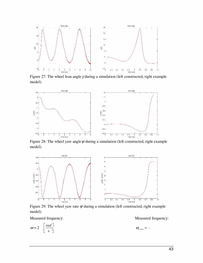
43
Figure 27: The wheel lean angle γ during a simulation (left constructed, right example
model).
Figure 28: The wheel yaw angleψ during a simulation (left constructed, right example
model).
Figure 29: The wheel yaw rate ψɺ during a simulation (left constructed, right example
model).
Measured frequency: Measured frequency:
2s
radω
≈
vω →∞ = -

44
Calculated frequency:
15.25
svω →∞
=
Experiment 4.) Forward velocity 2.25m
s
Figure 30: The wheel lean angle γ during a simulation (left constructed, right example
model).
Figure 31: The wheel yaw angle ψ during a simulation (left constructed, right example
model).

45
Figure 32: The wheel yaw rate ψɺ during a simulation with a [ ]0.1 / sinitial
radψ =ɺ (left
constructed, right example model).
Measured frequency: Measured frequency:
8.9s
radω
≈
8.5s
radω
≈
Calculated frequency:
110.27
sv
ω →∞
=
Experiment 5.) Forward velocity 3.5m
s
Figure 33: The wheel lean angle during a simulation (left constructed, right example
model).
Figure 34: The wheel yaw angle ψ during a simulation (left constructed, right example
model).

46
Figure 35: The wheel yaw rate ψɺ during a simulation with a [ ]0.1 / s
initialradψ =ɺ (left
constructed, right example model).
Measured frequency: Measured frequency:
14.7s
radω
≈
15.3s
radω
≈
Calculated frequency:
115.97
sv
ω →∞
=
2.11 Parameter variations
In the previous measurement data the instability increased with time. For the following
experiment we will start with the initial tyre parameters and focus on measurement
instabilities due to parameter variations. Therefore a simple experiment with different
tyre parameters is set up. By multiplying the tyre parameters with a factor ½ or 2 we
should get an idea of their influence. Furthermore an experiment with different
integration methods is performed.
2.11.1 Different tyre parameters
For this experiment the same tyre parameters are used as for the case where the model of
Sharp is compared with the constructed tyre. Furthermore one specific case (vcritical) is
taken from the experiment and tested.
• Mass: 25.6 [kg]
• Wheel radius: 0.3190 [m]
• Inertia matrix:
0.3 0 0
0 0.58 0
0 0 0.3
[kgm2]
• Gravity: 9.81 [m/s2]

47
The motorcyle tyre stiffness are taken from [19]:
• Vertical tyre stiffness: k=115000 [N/m]
• Damping: c=500 [Ns/m]
• Longitudinal tyre stiffness: Fx
C =20000 [N]
• Lateral tyre stiffness: Fy
C =20000 [N]
The initial conditions for the experiment are defined as follows. Where the yaw rate was
also sinusoidal but with a different amplitude and frequency.
• Forward velocity (critical speed): 1.15 m
s
• Angular roll velocityspin
ω : 3.61 s
rad
• Yaw rate: 0.1 s
rad
2.11.2 Simulation results
In our first vehicle experiment we consider simulated low tyre stiffness. In the second
experiment we repeat the modeling from the first experiment, but now with simulated
high tyre stiffness. Each time the damping, vertical, longitudinal and lateral tyre stiffness
are multiplied with a factor ½ and 2 respectively. At first the measured data of the initial
tyre parameters is shown and secondly the two adjusted ones.
The first set of figures show the speed of the center of mass (cm). Especially in these
figures the growing instability is clearly visible.
Figure 36: Wheel centre of mass with an initial forward velocity of 1.15 [m/s].
48
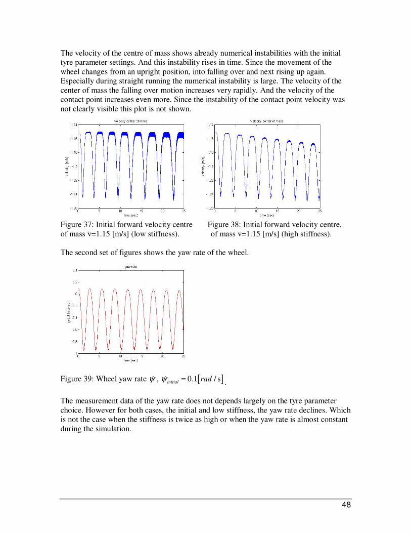
The velocity of the centre of mass shows already numerical instabilities with the initial
tyre parameter settings. And this instability rises in time. Since the movement of the
wheel changes from an upright position, into falling over and next rising up again.
Especially during straight running the numerical instability is large. The velocity of the
center of mass the falling over motion increases very rapidly. And the velocity of the
contact point increases even more. Since the instability of the contact point velocity was
not clearly visible this plot is not shown.
Figure 37: Initial forward velocity centre Figure 38: Initial forward velocity centre.
of mass v=1.15 [m/s] (low stiffness). of mass v=1.15 [m/s] (high stiffness).
The second set of figures shows the yaw rate of the wheel.
Figure 39: Wheel yaw rate ψɺ , [ ]0.1 / sinitial
radψ =ɺ .
The measurement data of the yaw rate does not depends largely on the tyre parameter
choice. However for both cases, the initial and low stiffness, the yaw rate declines. Which
is not the case when the stiffness is twice as high or when the yaw rate is almost constant
during the simulation.

49
Figure 40: Wheel yaw rate ψɺ (low stiffness), Figure 41: Wheel yaw rate ψɺ (high
[ ]0.1 / sinitial
radψ =ɺ . stiffness), [ ]0.1 / sinitial
radψ =ɺ .
The third and final set of figures show the lateral slip angle.
Figure 42: Wheel lateral slip angle α .
The measurement data of the lateral slip angle depends largely on the tyre parameter
choice. Regardless of the noisy behaviour of the measurement data, Figure 42 clearly
shows that an increase of the stiffness results in a ill conditioned systems.
Figure 43: Wheel lateral slip angle α Figure 44: Wheel lateral slip angle α
(low stiffness). (high stiffness).
50
2.12 Concluding remarks
In the described experiments we considered low and high tyre stiffness. In both
experiments there was a significant difference when altering the tyre parameters. Another
experiment was performed in order to take a closer look at the separate tyre parameters.
Changing only the vertical tyre stiffness seemed to had little influence on the measured
data. Although the change in undamped natural frequency was visible in the vertical force,
which is a penalty for the penetration of the contact point through the road plane.
Variations in the longitudinal and lateral tyre stiffness however were clearly visible.
Nevertheless for a good impression of the influence we altered the tyre parameters at
once.
2.13 Integration methods
The next step is to investigate the integration performance of the SimMechanics toolbox
and for this we performed a simulation. The differences in the computation time between
the solvers are more obvious as complexity of the model increases. This is probably
caused by the mathematical model that has to be derived by the software before the
integration of the ordinary differential equation system can begin.
Furthermore SimMechanics provides 4 types of motion analysis. The default is the
forward dynamics type:
1) Forward dynamics
2) Linearization
3) Trimming
4) Inverse dynamics
The modes corresponding to these types of analysis are:
• Forward dynamics
i. Computes the positions and velocities of a system’s bodies at each time step,
given the initial positions and velocities of its bodies and any forces applied to
the system.
• Forward dynamics
i. Computes the effect of small perturbations on system motion through the
Simulink linmod command.
• Trimming
i. Enables the Simulink trim command to compute steady-state solutions of system motion.
• Inverse dynamics
i. Computes the forces required to produce a specified velocity for each body of an
open-loop system.
• Kinematics
i. Computes the forces required to produce a specified velocity for each body of an
closed-loop system.
A SimMechanics simulation interprets the machine’s purely mechanical aspects through
machine assembly and a constraint solver. Simulink controls the purely mathematical
aspects of the simulation through the chosen Simulink solver. A SimMechanics model

51
uses one of the ordinary differential equation solvers of Simulink to solve a system’s
equations of motion.
The equations of motion for an arbitrary system [20].
( )=q H q vɶɺ (2-101)
( ) ( ) ( ) ( ), , ,T T
t t= +M q v f q v H q G q λɶɺ (2-102)
( ), 0g t =q (2-103)
Equation (2-101)expresses the kinematic relationship between the derivatives of the
configuration variables q and the velocity variables v. In the most simple cases Hɶ is the
identity matrix. The second equation (2-102) is the motion equation with the positive
definite mass matrix M, the acceleration vɺ , the contribution of the centrifugal, Coriolis
and external forces f, and the contribution of reaction forces due to kinematic constraints
which is expressed by the last term on the right side. Finally equation (2-103) represents
kinematical constraints between the configuration variables.
The main problem arising from equations (2-101) and (2-103) is that they form an index-
3 differential algebraic equation (DAE) because of the constraints in equation (2-103) .
Currently, Simulink is designed to simulate systems described by ODE’s and a restricted
class of index-1 DAE’s, so the multibody dynamics problem is not solvable directly.
In order to avoid the presence of constraints the differential algebraic system of equations
can be transformed into a system of ordinary differential equations. This can be achieved
through techniques such as constraint regularization or constraint reduction [23]. The
approach taken by SimMechanics is to differentiate the constraint equation (2-103) twice
and solve for the Lagrange multiplier λ. Near singularities of the mechanism, i.e. near
points where the number of independent constraint equations is decreased and the
solution for λ is no longer unique, numerical difficulties arise. To deal with this problem,
the user can choose between two solvers. One, based on Cholesky decomposition (the
default), which is generally faster, and one based on QR decomposition.
Coordinate Projection is used after each time step. The computed solution n
qɶ of time-step
tn is projected on the invariant manifold qn, given by g(qn, tn) = 0. This prevents the
solution from drifting away. For example, the projection approach is appropriate for a
one-step method used to compute an approximate solution at time tn+1 from a solution at
tn. The step size is h, and tn+1 tn+h Finally, stabilization is based on adding stabilization
parameters to the reduced ODE, which makes it more attractive to the manifold.
The SimMechanics user has the choice between coordinate projection and stabilization.
Coordinate projection is more exact, while the stabilization algorithms are faster and
suitable for real-time applications.

52
2.13.1 Solver type with a fixed time step
The Dormand-Prince solver (ode45), with a variable time step, that Simulink uses by
default works well for many mechanical systems. However since the wheel model is slow
and inaccurate we tried a different solver with a fixed time step. Moreover we want to
perform real time Hardware in the loop simulation for that reason the time to integrate
one time step must be predictable.
The initial conditions for the experiment are defined as follows:
• Forward velocity (critical speed): 2.25m
s
• Angular roll velocityspin
ω : 3.61 s
rad
• Yaw rate: 0.1 s
rad
• Fixed step size: 0.01 - 0.0001 [ ]s
Figure 45: Wheel yaw rate ,ψɺ Figure 46: Wheel yaw rate ,ψɺ
time step=1e-3
, [ ]0.1 / sinitial
radψ =ɺ time step=1e-4
, [ ]0.1 / sinitial
radψ =ɺ
A first attempt with a fixed time step is performed with the Runge-Kutta solver (ode4),
based on a time step of 1e-2
seconds. This simulation data could not be shown due to a
simulation crash. Figure 23 shows a fixed time of 1 millisecond. In this case the
simulation runs normal. However the signal shows a noisy behaviour during the entire
simulation time. Decreasing the simulation time with a factor 10 shows much better
results. There are no spikes visible in figure 24 and the yaw rate is slightly decreasing.
One major disadvantage of this time step is the total simulation time, because this can be
easily run up to 5 minutes.

53
3. SimMechanics joint block modeling
Several problems are encountered during the simulation of the wheel model. One of these
problems was a singularity error. In most simulation diagnostic errors, the error was
caused by the custom joint block. This type of error will be discussed in more detail,
based on the previous modeled wheel. Finally, two solutions to this problem are given
and a comparison is made.
3.1 Euler angles
In rigid body mechanics we need to keep track of points for each body. The motion of
such a body can be decomposed into a translation and a rotation. Here we focus on the
rotational part. A number of such sets of parameters have been described in literature, but
the most common and useful way to describe the rotation (the change in orientation) of
rigid bodies are the Euler or Eulerian angles. The body can be oriented with respect to the
space fixed coordinate system by means of three successive rotations. However these
rotations are limited.
These limitations or angle ranges are given below:
• x and z range are defined modulo 2π radians. A valid range could be [-π, π). • y range covers π radians (but can't be said to be modulo π). For example could be
[0, π] or [-π/2, π/2].
In case of the xyz-convention the y-axis, as stated in the angle ranges, is limited in its
rotational movement. For the xyz-convention this means we have to avoid large rotations
on the second position. This will be explained in the next paragraph.
Desired sequence.
When building a custom joint block for vehicle modeling we can firstly state that, the
rolling motion of the wheel has to rotate around the y-axis (roll). Therefore this axis has
to be able to rotate over 2π radians. Secondly the x-axis (lean) - since if the lean angle is
90 degrees or larger the wheel would be parallel with the road surface. Finally when the
wheel is spinning around the z-axis this rotation could be large as well. This results in the
following Euler angle sequence z-x-y.
Brief description of sequence illustration
The various stages of this convention are often illustrated with respect to the space fixed
coordinate system by means of three successive rotations. However these stages and the
corresponding drawings are rather complex. Therefore we used another way of
illustrating this sequence. Namely the sequence of rotations about different axes by the so
called cans in series [29]. Each rotation about an axis is represented by a pair of cans
rotating with respect to one another. The drawing of the cans in series can be looked upon
as an exploded view of the materialization of the Euler angles and by such demonstrates
the proper operation of the process. The different stages of the intermediate coordinate
system are now located at the end of the first two pairs of cans. For the z-x-y sequence as
illustrated in Figure 47 this means that between the z & x ‘cans’ the first coordinate

54
system is placed. The second one is placed between x & y ‘cans’ and the last is placed on
top of the z ‘can’.
Figure 47: Euler angle sequence with ‘cans’ in series: z-x-y. As illustrated in this figure
large rotations occur around the wheel rolling axis which is located on the third position
of the Euler sequence.
3.2 Angle sequence in SimMechanics
Choosing this angle sequence in SimMechanics appeared to be difficult. The relative
coordinates approach where a body is initially given zero degrees of freedom, enables the
designer to use different kinds of joint blocks. The problem however with these joint
blocks is that at first we could not locate this rotational representation in the
documentation. A closer look learned that there are various rotation representations,
which was very useful but one still does not know which type of joint is corresponds with
what representation. In this case we were interested in the custom joint block, which is
described next.
A Joint block represents the relative degrees of freedom between two bodies, not the
bodies themselves. Any Joint block must be connected to two body blocks, the base and
the follower. All Joints have two connector ports for these connections, defining the
direction of joint motion (base to follower).
Figure 48: schematic overview of input and output parameters. Where te focus lies on the
custom joint block.

55
Each side of the Joint block is connected to these Body blocks at a Body coordinate
system (CS) port. Furthermore the base (B)-follower (F) Body sequence determines the
sense of positive motion:
• Positive translation is the follower moving in the direction of the translation axis.
• Positive rotation is the follower rotating in the right-hand-rule about the rotation
axis.
By selecting a custom joint block, one gets the scheme below. The specification of the
joint primitive axes, if any, take place in the joint dialog. One gets by default one
rotational axis and can “add”, prismatic and rotational, primitives to the block.
Figure 49: Scheme of custom joint. Where five degrees of freedom are added (R2, R3 P1,
P2 and R3).
It turned out that the sequence in which they are presented in the custom joint block
equals the Euler angle sequence. So by adding the primitives R1, R2 and R3 in the custom
joint block, one unintentionally defines the rotation sequence of the body, although the
primitive name is of no influence. For the ‘Axis of Action’ in the custom joint this means
that the first primitive equals the first body rotation.
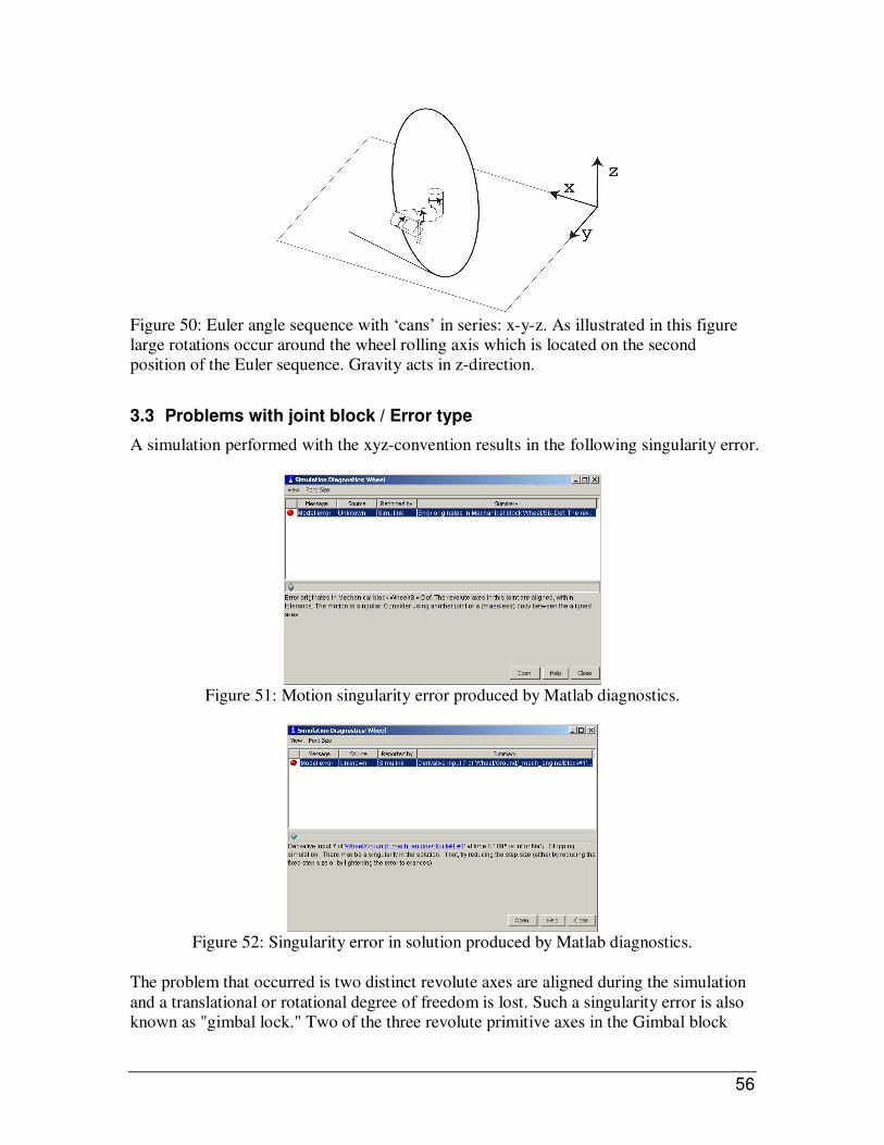
56
Figure 50: Euler angle sequence with ‘cans’ in series: x-y-z. As illustrated in this figure
large rotations occur around the wheel rolling axis which is located on the second
position of the Euler sequence. Gravity acts in z-direction.
3.3 Problems with joint block / Error type
A simulation performed with the xyz-convention results in the following singularity error.
Figure 51: Motion singularity error produced by Matlab diagnostics.
Figure 52: Singularity error in solution produced by Matlab diagnostics.
The problem that occurred is two distinct revolute axes are aligned during the simulation
and a translational or rotational degree of freedom is lost. Such a singularity error is also
known as "gimbal lock." Two of the three revolute primitive axes in the Gimbal block
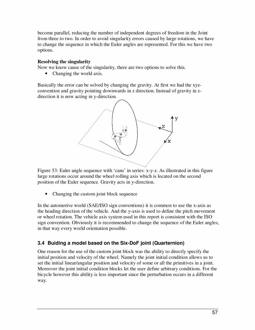
57
become parallel, reducing the number of independent degrees of freedom in the Joint
from three to two. In order to avoid singularity errors caused by large rotations, we have
to change the sequence in which the Euler angles are represented. For this we have two
options.
Resolving the singularity
Now we know cause of the singularity, there are two options to solve this.
• Changing the world axis.
Basically the error can be solved by changing the gravity. At first we had the xyz-
convention and gravity pointing downwards in z direction. Instead of gravity in z-
direction it is now acting in y-direction.
Figure 53: Euler angle sequence with ‘cans’ in series: x-y-z. As illustrated in this figure
large rotations occur around the wheel rolling axis which is located on the second
position of the Euler sequence. Gravity acts in y-direction.
• Changing the custom joint block sequence
In the automotive world (SAE/ISO sign conventions) it is common to use the x-axis as
the heading direction of the vehicle. And the y-axis is used to define the pitch movement
or wheel rotation. The vehicle axis system used in this report is consistent with the ISO
sign convention. Obviously it is recommended to change the sequence of the Euler angles,
in that way every world orientation possible.
3.4 Buiding a model based on the Six-DoF joint (Quarternion)
One reason for the use of the custom joint block was the ability to directly specify the
initial position and velocity of the wheel. Namely the joint initial condition allows us to
set the initial linear/angular position and velocity of some or all the primitives in a joint.
Moreover the joint initial condition blocks let the user define arbitrary conditions. For the
bicycle however this ability is less important since the perturbation occurs in a different
way.

58
The Six-DoF block represents a composite joint with three translational degrees of
freedom as three prismatic primitives and three rotational degrees of freedom as one
spherical primitives. There are no constraints among the primitives. Unlike Bushing, Six-
DoF represents the rotational degrees of freedom as one spherical, rather than as three
revolutes. The motion of prismatic primitives is specified in linear units. The motion of
spherical primitives is specified by a dimensionless quaternion. To be certain that these
two joint block options had the same result an experiment was performed.
3.5 Wheel comparison between Custom and Six-DoF joint at 2.5 [m/s]
In the previous wheel experiment we used an initial velocity around the z-axis (yaw), in
order to perturb the motion. But as explained for the Six-DoF joint it is not possible to
specify initial conditions in the joint block. Therefore we had to use another approach to
perturb the wheel model in order to look at the oscillatory trajectory. This perturbation is
performed with the use of a lateral force on the wheel center.
Remark: for this experiment the lateral perturbation force was 5 [N]. And is applied from
1-2 seconds.
Figure 54: The wheel yaw rate of the custom joint Figure 55: The wheel yaw rate Six-
DoF joint block.
17.3780945
sλ
=
1
7.3859002s
λ
=
As before the same procedure for data fitting is used. This procedure will be explained in
paragraph 4.7.
3.6 Concluding remarks
Depending on the purpose one can choose a Six-DoF or a custom joint block. Though for
the latter one has to be careful in defining the order of primitives. Problems due to an
incorrect primitive sequence are mainly caused by: singularities.

59
4. Bicycle
4.1 Introduction to the bicycle model
Now the wheel model is completed and the singularities solved. We can continue with
the modeling of a bicycle. One of the most basic mechanical models of a bicycle is
described in [28]. This Whiple model consists of four rigid bodies, i.e. the rear frame
with the rider body rigidly attached to it, the front frame being the front fork, the front an
rear wheels. Furthermore in [27] this model is described in detail and known as the
bicycle benchmark. The advantage of the benchmark is that anyone working in the areas
of bicycle or motorcycle handling or control can use these equations directly or verify
their own underlying equations. In this case the detailed description enables us to analyze
and validate the SimMechanics model regarding stability.
4.2 Construction of the bicycle model
With the use of sensors we can measure the variables and sent this data to the Matlab
workspace for further processing. This can be done by adding Sensor blocks and Joint
Initial Condition blocks. With their help, a model which is functionally completely
equivalent to the Whiple model can be build. The Joint Initial Condition blocks let the
user define arbitrary initial conditions, and the Joint Sensor blocks measure the position,
velocity, and acceleration of the two independent motion variables.
If desired, the forces and torques transmitted by the joints can be sensed, too.
Figure 56: Configuration and dynamic variables. The 7-dimensional accessible
configuration space is parameterized here by the x and y coordinates of the rear contact
P, measured relative to a global fixed coordinate system, and 5 angles represented by a
sequence of hinges (gimbals). The hinges are drawn as a pair of cans which rotate with
respect to each other. [27].
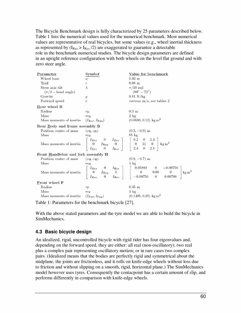
60
The Bicycle Benchmark design is fully characterized by 25 parameters described below.
Table 1 lists the numerical values used for the numerical benchmark. Most numerical
values are representative of real bicycles, but some values (e.g., wheel inertial thickness
as represented by (IRxx > IRyy /2) are exaggerated to guarantee a detectable
role in the benchmark numerical studies. The bicycle design parameters are defined
in an upright reference configuration with both wheels on the level flat ground and with
zero steer angle.
Table 1: Parameters for the benchmark bicycle [27].
With the above stated parameters and the tyre model we are able to build the bicycle in
SimMechanics.
4.3 Basic bicycle design
An idealized, rigid, uncontrolled bicycle with rigid rider has four eigenvalues and,
depending on the forward speed, they are either: all real (non-oscillatory); two real
plus a complex pair representing oscillatory motion; or in rare cases two complex
pairs. (Idealized means that the bodies are perfectly rigid and symmetrical about the
midplane, the joints are frictionless, and it rolls on knife-edge wheels without loss due
to friction and without slipping on a smooth, rigid, horizontal plane.) The SimMechanics
model however uses tyres. Consequently the contacpoint has a certain amount of slip, and
performs differently in comparison with knife-edge wheels.

61
4.4 Eigenvalue analysis
Analysis of the eigenvalues and their corresponding eigenvectors reveals the
natural modes of the bicycle: the eigenmodes. See the plot below of eigenvalues for a
typical utility bicycle that demonstrates the common characteristics.
Figure 57: Eigenvalues λ from the linearized stability analysis for the benchmark bicycle
The solid lines correspond to the real part of the eigenvalues and the dashed line
corresponds to the imaginary part of the eigenvalues, in the forward speed range of
0 ≤ v ≤ 10 m/s [27].
At low forward speeds, starting at zero, the eigenvalues come in two positive and
negative pairs and represent the instability of an inverted pendulum. Depending on
the particular parameters of the bicycle, lean and steer can have the same or opposite
signs, which represent steering away from lean or towards lean, respectively. Also,
their rates are positive and so increasing. At sufficiently higher speed, the two positive
real eigenvalues commonly merge to form a complex conjugate pair with positive real
parts. This represents unstable oscillatory motion and is referred to as the weave mode.
The bicycle leans and steers from side to side.
As forward speed increases, the frequency of this weave increases, as is indicated by the
increasing magnitude of the imaginary parts of the complex conjugate eigenvalues. This
increase in magnitude becomes nearly linear with the increase in forward speed, and so
the wavelength of the weave is nearly constant.
For certain bicycle configurations, at a higher speed still, this pair crosses the real
axis and the weave motion becomes stable. This is the beginning of the range of
forward speeds for which the bicycle is self-stable. In the corresponding eigenvector, the
lean angle and steer angle have opposite signs, the bicycle is leaning and steering in the
same direction Of the two initially-negative eigenvalues, the smaller one corresponds to

62
the capsize mode. For many bicycle configurations, it becomes positive (unstable) at a
speed above the weave speed, marking the end of the self-stable range of speeds. In the
corresponding eigenvector, the lean angle and steer angle have opposite signs and the
bicycle is leaning and steering in the same direction. However, while lean rate is positive,
steer rate is negative. Finally, the eigenvalue initially most negative has an eigenvector
dominated by steer rate and represents the castor mode: the tendency of the front wheel to
steer in the direction the bicycle is moving. It only becomes more negative and so more
stable as forward speed increases.
4.5 Building the bicycle model
In the benchmark linearized equations of motion for the Whipple bicycle model are
presented, consisting of four rigid laterally-symmetric ideally-hinged parts: two wheels, a
frame and a front assembly. The wheels are also axisymmetric and make ideal knife-edge
rolling point-contact with the level ground. The mass distribution and geometry are
otherwise arbitrary. This conservative non-holonomic system has a 7-dimensional
accessible configuration space and three velocity degrees of freedom parameterized
by rates of frame lean, steer angle and rear-wheel rotation [27].
The first step of modelling is to describe the rigid parts and the joints connecting the parts,
where a part is described by its mass, inertia and orientation. Specifically, in the bicycle
model considered here the frame is constrained by a custom six-dof joint, which is driven
by a translational motion, and the wheels are constrained by rotational joints and driven
by a angular motion. The next step is the addition of internal force elements to represent
the tyre forces. The tyres are modelled with impact functions that switch on as soon as
the distance between the wheel centre and the tyre becomes less than the wheel radius.
With the aid of the bicycle parameters as stated in table 1 and the tyre model from
chapter 2 we are able to build the SimMechanics bicycle model. In the same way as the
tyre model, the body blocks and joints are placed in a Simulink window. A more detailed
description can be found in appendix c.
4.6 Problems with the bicycle model
After the bicycle model was build a few simulations were performed. However regardless
the initial speed or perturbing force the bicycle became instantly unstable. At first we
thought the error could be found in a misinterpretation of a sign convention of the front
and rear wheel. e.g. introducing a plus in the rear wheel and a correct minus sign in the
front wheel configuration, could result in a self exciter of the rear end. But this was not
the case. Since the error could not be found in the bicycle configuration or parameters, it
was presumably caused in the tyre model.
For the disk initially a rotational damper (around the z-axis) was build in the wheel model
for stability reasons. Namely, the wheel showed some kind of perpetual behaviour.
Therefore this damper was taken out of the model. This seemed to be the key to a
successful simulation. So we had to find out what the effect of such a damper had on
stability. Already in 1971 Sharp [24] introduced lag in the tyre side force by a first order

63
relaxation model, which seems of large influence on the dynamic behaviour of a
motorcycle.
In our case the use of a rotational damper seemed to destabilize the bicycle. This resulted
in the following conclusion. Using a damper for the turnslip according to (2-79)
leads to a model which is unstable. Another possibility is the use of a damper in
combination with a spring, in other words a relaxation length, also used for the
longitudinal and lateral stiffness (2-77), (2-78). Introducing a damper for a disk results in
a more realistic Euler disk behaviour. But it makes a bicycle unstable. Pacejka uses κ ∗[6,
Chapter 6], in order to overcome the shimmy effect and to increase the range of stability
or to decrease the unstable area of the shimmy. But in our case introducing turnslip
resistance does the exact opposite. When turnslip moments are incorporated as some kind
of a frictional damper, the bicycle becomes unstable. However in series with a spring,
resulting in a relaxation filter, the turnslip works properly.
4.7 Lateral pertubation (CG)
One side effect of a simulation performed in a idealistic world, such as SimMechanics, is
that the bicycle acts in an unstable equilibrium. Therefore the bicycle has to be brought
out of this equilibrium in order to perform stability measurements.
To overcome this problem we purposely initiated a dynamic response by applying an
impulse in lateral direction to the bicycles centre of gravity. The SimMechanics scheme
of this perturbation is depicted in Figure 58. The impuls consists of signal with unit
height , next this multiplied with a gain of 20 in order to get a force of 20 [N]. The
bicycle response to this perturbation was sufficiently for the measurements.
Figure 58: Scheme of perturbation signal, Figure 59: Block signal given by the signal
with the signal builder, gain and actuator builder in the Simulink toolbox.
To be sure all vertical dynamics are canceled out during a simulation the bicycle was
initially driving forward with the given velocity and after 4 till 6 seconds a lateral
perturbation force acted on the centre of gravity of the bicycle. As explained earlier the

64
lean and steer rate are used to determine the eigenvalues at a certain velocity. However
for a better visualization the lean is shown.
4.7.1 Bicycle comparison between Custom and Six-DoF joint at 4.292 [m/s]
Before continuing with the bicycle simululations, we wanted to make sure there is no
distinction between the SimMechanics custom and the Six-DoF joint. So the same
reasoning as for the disk was followed, in order to compare both joints. The same
procedure for data fitting as before is used, which is explained in paragraph 4.6.
Based on custom joint:
Measured lambda: 1
3.4363s
λ
=
(4-1)
Based on Six_DoF joint:
Measured lambda: 1
3.4386s
λ
=
(4-2)
Since the eigenvalue difference of both joints is in the order of 1/1000, we may conclude
that this is negligible.
4.7.2 Bicycle simulations
The variables that we wanted to measure for an adequate validation areδ the steer angle,
δɺ the steer angle rate, γ the lean (roll) angle,γɺ the lean (roll) angle rate, and v the
forward speed (which would range from 0 to 10 m/s). With these variables we could then
compare the measured values to the calculated values. Below four characteristic speeds
are discussed in more detail. In each case the lean and steer rate is shown, since the lean
rate was a very compact figure and needed some up scaling.
Energy conservation
When an uncontrolled bicycle is within its stable speed range, lean and steer
perturbations die away in a seemingly damped fashion. However, the system has no
true damping and conserves energy. The energy in the lean and steer oscillations is
transferred to the forward speed rather than being dissipated. As the forward speed
is affected only to second order, linearized equations do not capture this energy
conservation. [27].
First the unstable weave speed is taken followed by the stable weave.

65
Figure 60: Bicycle lean versus time Figure 61: Bicycle steer rate versus time
at an unstable weave velocity v=4.0 [m/s]. at an unstable weave velocity v=4.0 [m/s]
Figure 60 and Figure 61 represents the unstable oscillatory motion and is referred to as
the weave mode. The bicycle leans and steers from side to side. The increasing
(undamped behaviour) for lean and steer are in accordance with the linearized benchmark
model since this speed is located in the unstable speed region.
Figure 62: Bicycle lean versus time Figure 63: Bicycle steer rate versus time
at a stable weave velocity v ≈ 4.3 [m/s]. at a stable weave velocity v ≈ 4.3 [m/s].
Figure 62 shows a simulation of the weave speed at approximately 4.3 m/s. After the
perturbing force the bicycle shows a slightly damped oscillatory behaviour. The same
holds for the steer rate. As this typically speed is located in the stable speed region of the
bicycle this oscillatory behaviour will damp out.

66
Figure 64: Bicycle lean versus time Figure 65: Bicycle steer rate versus time
at capsize velocity v ≈ 6.0 [m/s] at capsize velocity v ≈ 6.0 [m/s]
With an increasing speed however, the bicycle stabilizing effect is increasing. As can be
seen in Figure 64. This speed is defined as the capsize motion at capsize speed and is
situated at approximately 6 m/s. At this the speed one can see there are only two
oscillations left in the lean.
Figure 66: Bicycle lean versus time Figure 67: Bicycle steer rate versus time
at a velocity v=8.0 [m/s] at a velocity v=8.0 [m/s]
Further increase of the speed leads to an unstable bicycle motion. Figure 66 shows that
after the perturbation, the oscillation is damped almost immediately. The lean and steer
however are increasing after seven seconds, causing the bicycle to fall over. Although the
SimMechanics bicycle model has deformable tyres, we can say that the eigenvalues at
this stage correspond reasonable with the benchmark.
4.7.3 Simulation challenges
In total sixteen runs were carried out starting from 3 to 10 [m/s], plus two typically
speeds. At a lower velocities (< 3 [m/s]) the bicycle was to unstable to be kept upright for
long enough to be able to carry out any form of test.
The lack of lateral dynamics in the motion of the bicycle at higher speeds due to the
stability of the bicycle presented a problem. The changes in sensor output for the freely

67
coasting bicycle were very small, making it difficult to fit any data. This also made it
difficult to locate the starting point and end point of the free coasting part of the
measurement. Figure 66 shows an example of such a simulation where the bicycle had
practically no lateral dynamics.
Perturbing the bicycle at a velocity of 4 m/s shows a clearly oscillatory behaviour of the
lean rate. However at increasing velocity (> 6 [m/s]) this oscillation is damped out very
rapidly as can be seen in Figure 66, even so fast it is not possible anymore to fit the
function. Increasing the perturbation force to 50 [N], and even 100 [N] did not give the
desired effect and mainly influenced the lean angle of the bicycle.
4.7.4 Steer rate
Due to the high damping in this speed region and the unstable steer rate data in figure 43
making it difficult to fit any data. For that reason another experiment was performed with
a perturbation on the steer. With the use of an actuator it is possible to apply a moment on
the steering axis. This is done in a similar way as for the saddle perturbation, the steer
perturbation is build. The SimMechanics scheme of this perturbation is depicted in Figure
68. Since the head tube is a revolute joint only one signal is needed, this in opposite to the
saddle perturbation where three input signals are used (3D force vector). Furthermore the
signal has a duration of 0.1 second and the applied torque ranges from 2-5 [Nm].
Dependently on the bicycle dynamics the torque was adjusted.
Figure 68: Scheme of perturbation signal Figure 69: Block signal given by the signal
with the signal builder, gain and actuator builder in the Simulink toolbox.
Since these simulations showed excellent results at higher speeds we decided to simulate
the lower speeds as well, in order to compare the results with the saddle perturbation.
However at decreasing speed (around 4 m/s) the steer influence is substantial. Resulting
in a unstable simulation. Nevertheless these lower speeds were already covered by the
saddle perturbation simulations.
Steer perturbation 8 m/s
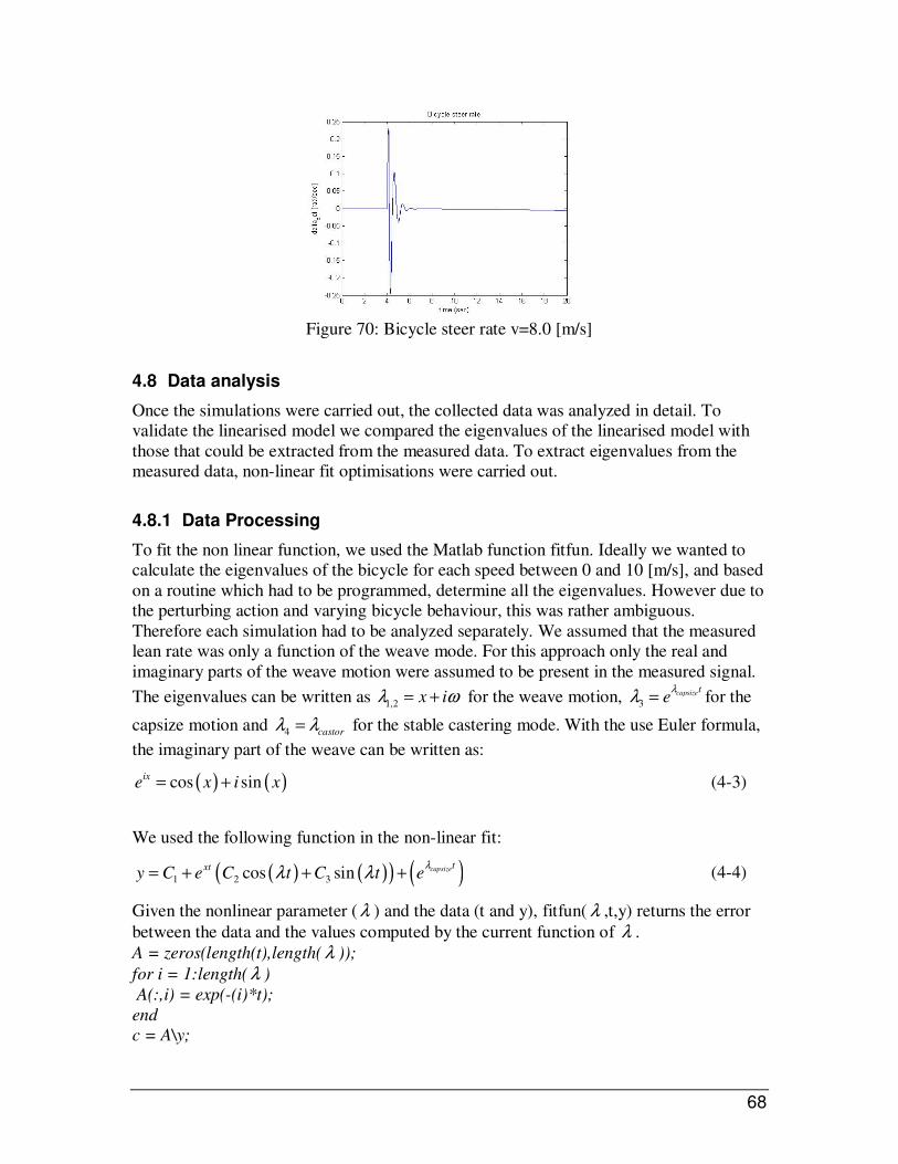
68
Figure 70: Bicycle steer rate v=8.0 [m/s]
4.8 Data analysis
Once the simulations were carried out, the collected data was analyzed in detail. To
validate the linearised model we compared the eigenvalues of the linearised model with
those that could be extracted from the measured data. To extract eigenvalues from the
measured data, non-linear fit optimisations were carried out.
4.8.1 Data Processing
To fit the non linear function, we used the Matlab function fitfun. Ideally we wanted to
calculate the eigenvalues of the bicycle for each speed between 0 and 10 [m/s], and based
on a routine which had to be programmed, determine all the eigenvalues. However due to
the perturbing action and varying bicycle behaviour, this was rather ambiguous.
Therefore each simulation had to be analyzed separately. We assumed that the measured
lean rate was only a function of the weave mode. For this approach only the real and
imaginary parts of the weave motion were assumed to be present in the measured signal.
The eigenvalues can be written as 1,2
x iλ ω= + for the weave motion, 3capsizet
eλ
λ = for the
capsize motion and 4 castorλ λ= for the stable castering mode. With the use Euler formula,
the imaginary part of the weave can be written as:
( ) ( )cos sinix
e x i x= + (4-3)
We used the following function in the non-linear fit:
( ) ( )( ) ( )1 2 3cos sin capsizetxty C e C t C t e
λλ λ= + + + (4-4)
Given the nonlinear parameter ( λ ) and the data (t and y), fitfun( λ ,t,y) returns the error
between the data and the values computed by the current function of λ .
A = zeros(length(t),length( λ ));
for i = 1:length(λ )
A(:,i) = exp(-(i)*t);
end
c = A\y;
69
z = A*c;
err = norm(z-y);
Castor mode
Since the castor mode is largely negative and its motion is damped out very rapidly,
minimizing the contribution to the total lean rate. We did not try to reconstruct
the caster mode from the gathered data. A similar situation was expected in the low speed
range (0 to 4 m/s) for the capsize eigenvalue. In this range the capsize eigenvalue is about
-3 and thus expected to be damped out swiftly. At higher speeds the capsize eigenvalue
becomes very small (initially slightly smaller than zero and from about 8 m/s
onwards, slightly larger than zero) thus the capsize mode is not heavily damped.
4.8.2 Interpolation
Interpolation is a method of constructing new data points from a discrete set of known
data points. This can be helpful when a data set presented that does not have the desired
resolution or is not equidistant. Interpolating a data set can also give the effect of
“smoothing” out a data set.
4.8.3 Mean zero
Although the lean and steer rate are taken for the non linear fit, we had to be sure the data
is averaged. For that reason the zero-mean of the simulation data had to be taken. To
calculate the mean and standard deviation of each column of the data. The next step is to
subtract the mean of each column. While it would be possible to do this using Matlab's
for loops, it would be very slow. It is much more efficient to use matrix operations. What
is required is to subtract a matrix where every entry in the ith column is the mean of that
column. This can be constructed by adding the following lines to the file:
e = ones(n, 1); (4-5)
y = x - e*mu; (4-6)
Now y is a data matrix where each variable has zero mean.
The results for the eigenvalue fits are shown in Figure 71 to Figure 74 for the lean and
steering rate respectively.

70
Figure 71: Bicycle lean v ≈ 4.3 [m/s] this figure shows such a fit process of the bicycle
after a saddle perturbation. First we tried to optimize the fit, this was done by changing
the time window and simply judging by eye how well the fit followed the data. Since at
this speed sufficient lateral dynamics are present, one can even take several time intervals
to make sure the error is small.
Figure 72: The non-linear fit of the lean. As illustrated with the rectangle in figure 49.
The red dots describe the function and onto these dots the assumed function is fitted.
Since this is a clear sinusoidal movement the fit follows the function very well.
Due to the lack of lateral dynamics at higher speeds, as described in paragraph 4.6.3, the
steer perturbation was introduced. As before the same method is used. Although the
oscillation is died out very rapidly, sufficiently data is available to capture one period.
The selected window and fit are shown in Figure 74.

71
Figure 73: Bicycle steer rate v=8.0 [m/s]. As in the previous fit procedure , the same
method is used. Again we first tried to optimize the fit, this was done by changing the
time window. However as can be seen the oscillation is damped out in a short time and
the sudden peaks caused by the perturbation have to be avoided in the fit. Thus a window
around six seconds was the best option.
Figure 74: The non-linear fit of the steer rate. As illustrated with the rectangle in figure
49, the figure on the right side shows the selected window. The red dots describe the
function and onto these dots the function is fitted.
Dependently on the simulation data an initial estimate of lambda (starting value) has to
be given. Like in this figure one has to careful choose this value, otherwise the fit is
inaccurate. However for this initial starting value we can use the linearized stability
analysis from [27] table 2.
Standard Deviation The Matlab fitfunction calculates the error of the fit. In order to use this in a more
quantitative way we have to look at the deviation. With this we are able to determine the
accuracy of a fit. These calculations are performed on simulations which showed a good
dynamic behaviour. Next we used the standard deviation of each fit as a measure for its
accuracy. The standard deviation for each fit was found by:
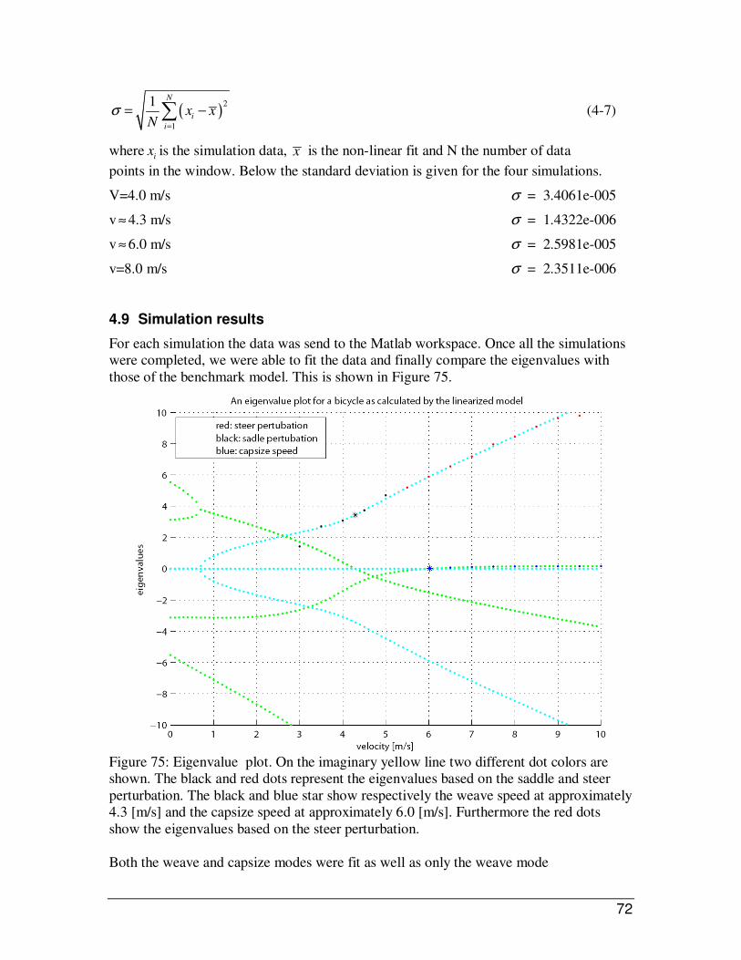
72
( )2
1
1 N
i
i
x xN
σ=
= −∑ (4-7)
where ix is the simulation data, x is the non-linear fit and N the number of data
points in the window. Below the standard deviation is given for the four simulations.
V=4.0 m/s σ = 3.4061e-005
v ≈ 4.3 m/s σ = 1.4322e-006
v ≈ 6.0 m/s σ = 2.5981e-005
v=8.0 m/s σ = 2.3511e-006
4.9 Simulation results
For each simulation the data was send to the Matlab workspace. Once all the simulations
were completed, we were able to fit the data and finally compare the eigenvalues with
those of the benchmark model. This is shown in Figure 75.
Figure 75: Eigenvalue plot. On the imaginary yellow line two different dot colors are
shown. The black and red dots represent the eigenvalues based on the saddle and steer
perturbation. The black and blue star show respectively the weave speed at approximately
4.3 [m/s] and the capsize speed at approximately 6.0 [m/s]. Furthermore the red dots
show the eigenvalues based on the steer perturbation.
Both the weave and capsize modes were fit as well as only the weave mode
73
on the measured data. At high speeds the calculated eigenvalues for the weave
motion matched those of the model very well. It was thought that the short
measurement window available during the low speed runs was the cause for the
poor comparison to the model at low speed. The lean angle signal turned out
to be the best signal for the non-linear fit.
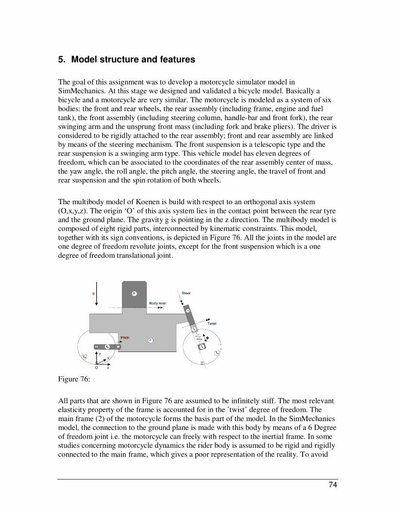
74
5. Model structure and features
The goal of this assignment was to develop a motorcycle simulator model in
SimMechanics. At this stage we designed and validated a bicycle model. Basically a
bicycle and a motorcycle are very similar. The motorcycle is modeled as a system of six
bodies: the front and rear wheels, the rear assembly (including frame, engine and fuel
tank), the front assembly (including steering column, handle-bar and front fork), the rear
swinging arm and the unsprung front mass (including fork and brake pliers). The driver is
considered to be rigidly attached to the rear assembly; front and rear assembly are linked
by means of the steering mechanism. The front suspension is a telescopic type and the
rear suspension is a swinging arm type. This vehicle model has eleven degrees of
freedom, which can be associated to the coordinates of the rear assembly center of mass,
the yaw angle, the roll angle, the pitch angle, the steering angle, the travel of front and
rear suspension and the spin rotation of both wheels.
The multibody model of Koenen is build with respect to an orthogonal axis system
(O,x,y,z). The origin ‘O’ of this axis system lies in the contact point between the rear tyre
and the ground plane. The gravity g is pointing in the z direction. The multibody model is
composed of eight rigid parts, interconnected by kinematic constraints. This model,
together with its sign conventions, is depicted in Figure 76. All the joints in the model are
one degree of freedom revolute joints, except for the front suspension which is a one
degree of freedom translational joint.
Figure 76:
All parts that are shown in Figure 76 are assumed to be infinitely stiff. The most relevant
elasticity property of the frame is accounted for in the ’twist’ degree of freedom. The
main frame (2) of the motorcycle forms the basis part of the model. In the SimMechanics
model, the connection to the ground plane is made with this body by means of a 6 Degree
of freedom joint i.e. the motorcycle can freely with respect to the inertial frame. In some
studies concerning motorcycle dynamics the rider body is assumed to be rigid and rigidly
connected to the main frame, which gives a poor representation of the reality. To avoid

75
too large differences between the model and reality, in this case the rider body is split up
in two parts. The lower segment of the rider body is assumed to be rigidly attached to the
main frame (2), the upper part (3) to rotate about an axis which is horizontal in the initial
condition, see Figure 76 This rotation is both sprung and damped. Furthermore, the rear
wheel (2) is connected to the main mass with a sprung and damped swing arm. This
massless swing arm makes it possible for the rear wheel to rotate around a point on
the main body and in the plane of symmetry, the ’pitch’ movement. Instead of a joint for
the pitch motion at the rear suspension, a swing arm can be used, which is also commonly
used in motorcycle models. The rear wheel (2w) is of course also given a Degree of
freedom in such a way that it is able to rotate around its own axle. At the front end of the
main mass the steer pivot is located. The steer body (1), twist body (1s), front unsprung
mass (1u) and front wheel (1w) together rotate as a whole relative to the main mass,
about an inclined steering axis. As said, the main elastic property of the frame has been
accounted for in the twist degree of freedom. The twist axis, which is perpendicular to the
steering axis, allows the twist body (1s), front unsprung mass (1a) and front wheel (1w)
to rotate out of the plane of symmetry of the motorcycle. Also this rotation is sprung and
damped. The front suspension is modelled as a translatory movement of the front
unsprung mass (1u) and front wheel (1w) perpendicular to the steering axis if no twist
angle is present. Again this movement is both sprung and damped. Finally, the front
wheel (1w) is given one degree of freedom, to be able to rotate around its spindle.
Figure 77:
Additional to the parts of the model that are depicted in Figure 77, the environment of the
motorcycle needs to be modelled. This comprises the road surface and the air through
which the vehicle moves. The road surface is assumed to be a flat and even plane
perpendicular to the direction of the local gravitational field. The air surrounding the
vehicle is assumed to be initially still relative to this ground plane. The motion of the
vehicle will give rise to both stationary and non-stationary forces acting on it. From these
forces only two components are regarded, the stationary drag and lift forces. The
direction and lines of application of these forces can be seen in Figure 77. The
motorcycle is modelled in such a way that the aerodynamic forces act at a specified point
of the main mass (2).

76
6. Conclusions
Objective of this thesis has been to build a motorcycle tyre model for real time purposes.
To evaluate the tyre behaviour a tyre model is developed in a Matlab/Simulink toolbox
SimMechanics. The parameters for the tyre models were at first estimated and later on
taken from motorcycle measurements.
Due to an initially ill conditioned system, several experiments showed noise and could
not be used. With the use of real motorcycle tyre parameters the simulation showed less
disturbance. However the simulation time were enormous, which could indicate a stiff
problem. Therefore another experiment was performed by varying the tyre stiffness. Next
relaxation lengths were implemented which improved the tyre behaviour. This enabled us
to perform some validations based on the rolling disk. At high speeds, the simulations
performed reasonable but at low speeds the data was still erratic and could not be used
analyzed.
Another problem was encountered with a singularity error. A closer look at the custom
joint structure learned that the problem could be found in assigning degrees of freedom
within the block. This appeared of great influence on the modeling. With this knowledge
we were able to build and test the bicycle model. The first indicative simulations showed
poor results caused by highly unstable bicycle behaviour. This however could be
addressed to the way the turnslip or path curvature was implemented. Resolving this
resulted into a successful simulation and from there on we could analyze and validate the
stability against the bicycle benchmark.
Due to insufficient simulation data at low speeds (< 3.5 [m/s]), no eigenvalues are
calculated. Moreover at high speeds the calculated eigenvalues for the weave motion, are
based on the steer perturbation and the lower speeds are based on the saddle pertuation.
However between 3.5 and 9.0 [m/s] the extracted eigenvalue clearly showed good
resemblance with linearised bicycle model, showing that the tyres have little influence on
the stability.

77
References:
[1] A MOTORCYCLE RIDING SIMULATOR FOR ASSESSING THE RIDING ABILITY AND FOR
TESTING RIDER ASSISTANCE SYSTEMS DSC 2006 Europe - Paris - October 2006 Vittore
Cossalter, Alberto Doria, Roberto Lot, Massimo Maso
[2] The stability of motorcycles under acceleration and braking. Limebeer, D.J.N. Sharp, R.S.,
Evangelou, S. Proc Inst Mech Engrs Vol 215 Part C
[3] Cossalter, Vittore, Doria Alberto, Lot, Roberto. “Development and validation of a motorcycle
riding simulator”. F2004F134
[4] V. Cossalter, A. Doria, D. Fabris, M. Maso. “Measurement and identification of the vibration
characteristics of motorcycle riders”. PROCEEDINGS OF ISMA2006
[5] Cocco, G. “Motorcycle design and technology” ISBN:88-7911-789-2
[6] H.B. Pacejka, Tyre and Vehicle dynamics, first edition. ISBN-13: 978-0768017021
[7] H.-J. Unrau, J. Zamow TYDEX-Format, Description and Reference Manual, Release 1.1,
Initiated by the International Tyre Working Group, July 1995.
[8] V. Engelson. Integration of Collision Detection with the Multibody System Library in
Modelica. Thesis, PELAB, IDA, Linkoping University, 2000.
[9] M. Otter, H. Elmqvist, J.Diaz Lopez. Collision Handling for the ModelicaMultiBody Library.
4th International Modelica Conference, pp.45-53, March 2004.
[10] Cornell Aaeronautical Laboratory, inc Buffalo, New York 14221. Bicycle dynamics tyre
characteristics and rider modeling. Cal report no. YA-3063-K-2 March 1972
[11] H. Goldstein, Classical mechanics, 2nd edition, Addison-Wesley, Reading, 1980
[12] ADAMS/Tyre. 2002 by Mechanical Dynamics, Incorporated. Part number: 120TIRG-01
[13] Y. Miyamarum, Development of a Riding Simulator and Its Prehistory, Preprint. JSME No.
59-00 (2000)
[14] W. Kading; “The Advanced Daimler-Benz Driving Simulator”, SAE 9530012, 1995.
[15] H. Soma and K. Hiramatsu; “Driving Simulator Experiment on Drivers’ Behaviour and
Effectiveness of Danger Warning Against Emergency Braking of Leading Vehicle”,
Proceedings of 16th ESV, Canada, 1998
[16] S. Chiyoda, K. Yoshimoto; Development of a motorcycle simulator using parallel
manipulator and head mounted display. 2002
[17] The MathWorks, Inc. SimMechanics 2 User’s Guide, March 2008.
http://www.mathworks.com
[18] Contact processing in the simulation of Clawar
[19] S. Evangelou and D.J.N. Limebeer. Lisp programming of the “Sharp 1994” motorcycle
model. Department of Electrical and Electrionic Engineering. Imperial College of Science

78
[20] M. Schlotter. Multibody System Simulation with SimMechanics. University of Canterbury,
May 2003
[21] G. D. Wood, D.C. Kennedy. Simulating Mechanical Systems in Simulink with SimMechanics.
The Mathworks, apple Hill Drive, Natick, MA, USA www.mathworks .com 91124v00
[22] A.L. Schwab “Dynamics of Flexible Multibody Systems. Small vibrations Superimposed on a
Genral Rigid Body Motion”. ISBN 90-6464-932-4
[23] M.Geradrdin, A Cardona. Flexible Multibody Dynamics. A Finite Element Approach. ISBN 0-
471-48990-5
[24] R. S. Sharp, \The stability and control of motorcycles", Jour. Mech. Eng. Sci., Vol. 13, No.5,
1971, pp. 316-329.
[25] The Effect of Tyre Modeling on the Stability Analysis of a Motorcycle E.J.H. de Vries and
H.B. Pacejka Delft University of Technology
[26] Moffatt, H. K., “Euler’s disk and its finite-time singularity,”
Nature 404 (2000), pp. 833–834.
[27] J. P. Meijaard, Jim M. Papadopoulos, Andy Ruina and A. L. Schwab Linearized dynamics
equations for the balance and steer of a bicycle: a benchmark and review
[28] Whiple, F.J.W. 1899 The stability of the motion of a bicycle. Quart. J. Pure Appl. Math. 30,
312-348
[29] A. L. Schwab, J. P. Meijaard. “How to draw Euler angles and utilize Euler parameters”
Proceedings of IDETC/CIE 2006 ASME 2006 International Design Engineering Technical
Conferences & Computers and Information in Engineering Conference September 10-13,
2006, Philadelphia, Pennsylvania, USA DETC2006-99307

79
APPENDIX A
Figure: The ISO sign conventions
1
1 The SimMechanics example model uses the SAE sign conventions where Y and Z are in opposite direction

80
APPENDIX B
The linearized equations of motion of a rolling disk with the eigenfrequencies as function
of the forward velocity [3]:
0( ) 0Mq Cvq K g q+ + =ɺɺ ɺ
The linearized state equations:
2 20 0 0 0
0 1 1 0 0 1
Mvmr mr mgr
Mr
ψ
γ
α ψ β ψ ψ
α γ β γ γ
+ + = + + −
ɺɺ ɺ
ɺɺ ɺ
Dimension analysis with m=1 g=1 and r=1. Times scales with rg
and speed with gr :
( )00 0 0
1 00 1 0 1
Mv
M
ψ
γ
βα ψ ψ ψ
βα γ γ γ
+ + = − ++ −
ɺɺ ɺ
ɺɺ ɺ
Characteristic equation:
( ) ( )
( ) ( )( )( )
2 4 2 2 2 2
2 2 2
0
1 1 0
v v
v
α α λ β α β λ
λ α α λ β β α
+ + − + =
+ + + − =
The eigenvalues:
( )( )
2
2
0
1
1
v
λ
β β αλ
α α
=
+ −=
+
The frequency above the critical velocity can be calculated as:
( )( )
21
1critv v
vβ β αω
α α>
+ −=
+
Limit cases:
( )
( )( )
10
1
1
1
v
v v
λα
β βω
α α
= = ±+
+= ∞ = ⋅
+
The scaling from the dimensionless quantity.
Time scales with: [ ]secr
g=

81
The disk radius with [ ]r m= and the eigenfrequency:
[ ]ω = −
1sec
ω =
( )1criticalv
α
β β=
+
For determining the critical speed we need to have the factors α and β :
2
0 0
0 0
0 0
I mr
α
β
α
=
The inertia for a disk:
0.25 0 0
0 0.5 0
0 0 0.25
diskI
=
So transferring the disk into non dimensionless:
( )( )
21
1critv v
vβ β αω
α α>
+ −=
+
Filling in the values for the disk inertia:
( )( )
1 11 122 2
1 1 514 4
critv v v vω >
+= ⋅ = ⋅
+
Rearranging and substitution of the earlier stated yields:
12 1
5
rv
g grω = ⋅ ⋅
This results in the scaling factor:
12
5
v
rω = ⋅ 1
sec

82
APPENDIX C
Creating SimMechanics Models
The most important special terms used in this guide are summarized in the Understanding
Mechanical Concepts chapter in Summary of Technical Vocabulary. In the online tutorials, special
terms occurring in the text (such as coordinate system and reference frame) are linked to
definitions in the Glossary.
Essential Steps to Build a Model [17]
The same basic procedure is used for building a SimMechanics model regardless of its
complexity. The steps are similar to those for building a regular Simulink model. More
complex models add steps without changing these basics.
Figure 78: SimMechanics representation of bicycle model (Top level)
Let us have a closer look at this diagram. Every block corresponds to one mechanical
component. The properties of the blocks can be entered by double-clicking on them. Next
all the different blocks and there properties are visualized.
1. Select Ground, Body, and Joint blocks. From the Bodies and Joints libraries, drag
and drop the Body and Joint blocks needed to represent your machine, including
at least one Ground block, into a Simulink model window.

83
Figure 79: SimMechanics representation of ‘Env_Ground_Six-DoF’ block as shown in
the bicycle top level.
Positioning and connecting blocks: The Joint and Body blocks are placed in proper relative position in the model window
and connected right order. The essential result of this step is creation of a valid tree block
diagram made of:
• Machine Env — Ground — Joint — Body — Joint — Body — ... — Body
Figure 80: Properties of the ‘env’ block parameters machine environment. The Machine
Environment block represents your machine’s mechanical settings.
Figure 81: Properties of the ground block. Ground blocks represent immobile ground
points at rest in absolute (inertial) space.
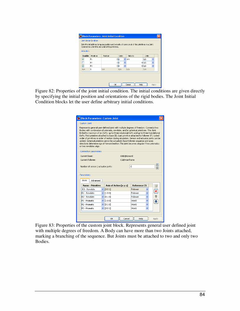
84
Figure 82: Properties of the joint initial condition. The initial conditions are given directly
by specifying the initial position and orientations of the rigid bodies. The Joint Initial
Condition blocks let the user define arbitrary initial conditions.
Figure 83: Properties of the custom joint block. Represents general user defined joint
with multiple degrees of freedom. A Body can have more than two Joints attached,
marking a branching of the sequence. But Joints must be attached to two and only two
Bodies.

85
Figure 84: Properties of the body mainframe block. Represents a user defined rigid body.
In the Body block the mass properties (masses and moments of inertia) are specified, as
well as the position and orient of the Body and Grounds relative to the World coordinate
system (CS) or to other CSs.
Figure 85: Properties of the joint initial condition. The initial conditions for the wheel are
given directly by specifying the velocity of the rigid body.
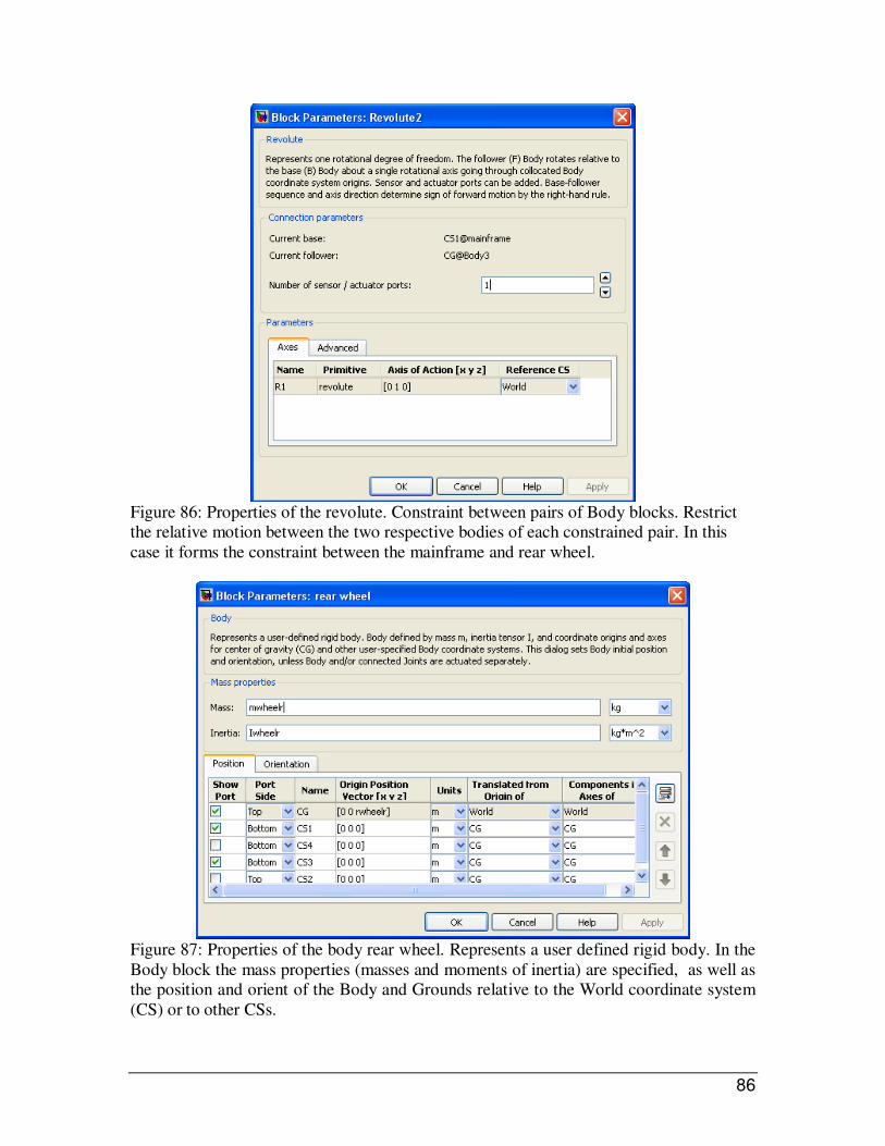
86
Figure 86: Properties of the revolute. Constraint between pairs of Body blocks. Restrict
the relative motion between the two respective bodies of each constrained pair. In this
case it forms the constraint between the mainframe and rear wheel.
Figure 87: Properties of the body rear wheel. Represents a user defined rigid body. In the
Body block the mass properties (masses and moments of inertia) are specified, as well as
the position and orient of the Body and Grounds relative to the World coordinate system
(CS) or to other CSs.

87
Actuator and Sensor blocks connect SimMechanics blocks to non-SimMechanics
Simulink blocks. SimMechanics blocks cannot be connected to regular Simulink blocks
otherwise. Actuator blocks take import signals from normal Simulink blocks (for
example, from the Simulink sources library) to actuate motion.
The Joint Sensor blocks measure the position, velocity, and acceleration of the two
independent motion variables.

88
Figure 88: SimMechanics representation of tyre model (overview). The structure of this
tyre model is illustrated in detail further on.

89
Figure 89: Properties of the headtube (revolute). Constraint between pairs of Body
blocks. Restrict the relative motion between the two respective bodies of each
constrained pair. In this case it forms the constraint between the mainframe and front
fork.
Figure 90: Properties of the front fork. Represents a user defined rigid body. In the Body
block the mass properties (masses and moments of inertia) are specified, as well as the
position and orient of the Body and Grounds relative to the World coordinate system
(CS) or to other CSs.

90
Figure 91: Properties of the joint initial condition. The initial conditions are given directly
by specifying the initial position and orientations of the rigid bodies. The Joint Initial
Condition blocks let the user define arbitrary initial conditions.
Figure 92: Properties of the revolute. Constraint between pairs of Body blocks. Restrict
the relative motion between the two respective bodies of each constrained pair. In this
case it forms the constraint between the front fork and front wheel.
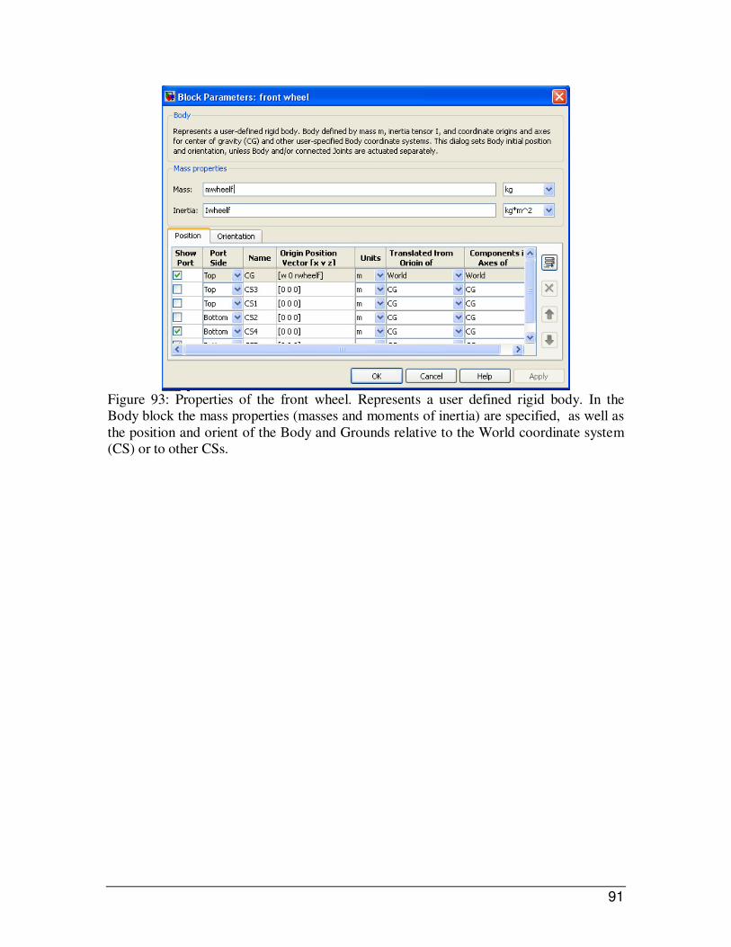
91
Figure 93: Properties of the front wheel. Represents a user defined rigid body. In the
Body block the mass properties (masses and moments of inertia) are specified, as well as
the position and orient of the Body and Grounds relative to the World coordinate system
(CS) or to other CSs.

92
Figure 94: SimMechanics representation of front tyre model (overview).

93
Figure 95: Represents the calculation of the material contact speed.
Figure 96: Represents the calculation of the vertical force.
Figure 97: Represents the calculation of the different vector calculations as discussed in
chapter 2.
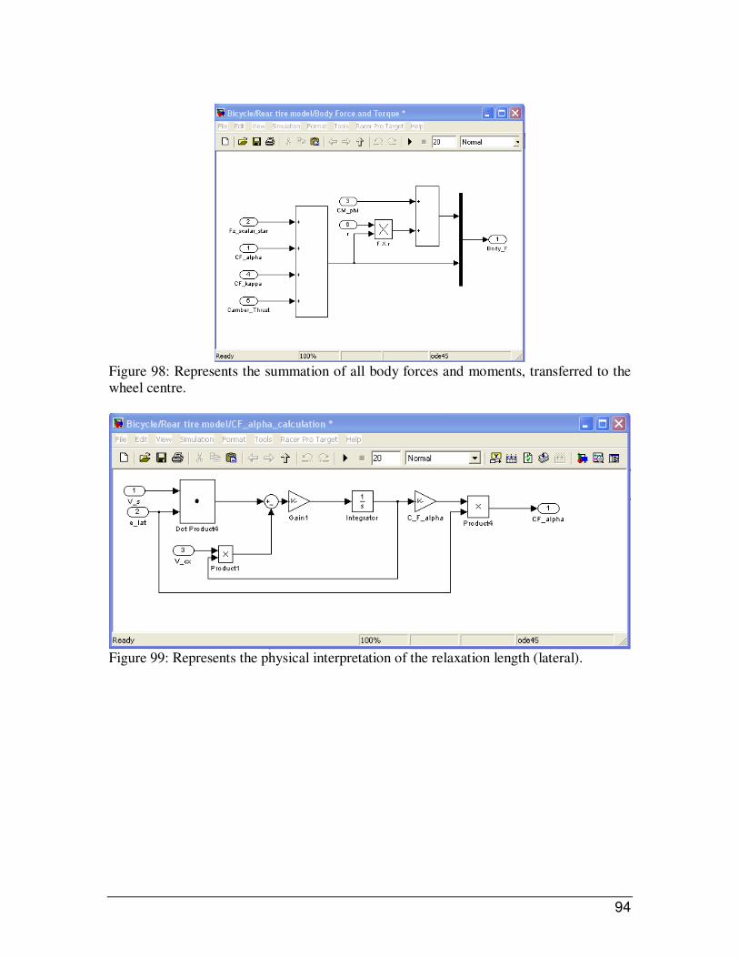
94
Figure 98: Represents the summation of all body forces and moments, transferred to the
wheel centre.
Figure 99: Represents the physical interpretation of the relaxation length (lateral).

95
Figure 100: Represents the physical interpretation of the relaxation length (longitudinal).
Figure 101: Represents a relaxation length for the turnslip or pathcurvature.
Figure 102: Represents the calculation of the camber or lean thrust.

96
Sensor blocks: To measure the motion of a body, a connection has to be made with one or more
Simulink Scope blocks to the model. The SimMechanics library of Actuators and Sensor
blocks gives you the means to input and output Simulink signals to and from
SimMechanics models. Furthermore it is possible to apply forces and motions with an
actuator body.
The Body, Joint, and Constraint/Driver blocks need to be reconfigure (by adding ports) to
accept Sensor and Actuator connections. Specify control signals (applied forces/torques
or motions) through Actuators and measure motions through Sensors.
Figure 103: Block parameters of a body actuator. Actuator blocks specify forces,
motions, variable masses and inertias, or initial conditions applied to bodies, joints, and
drivers.
Figure 104: Block parameters of a joint sensor. Sensor blocks measure the forces on and
motions of bodies, joints, and drivers.