A Sequential Game Model of Sports Championship … SEQUENTIAL GAME MODEL OF SPORTS CHAMPIONSHIP...

A SEQUENTIAL GAME MODEL OF SPORTS CHAMPIONSHIP SERIES: THEORY AND ESTIMATION

Christopher Ferrall and Anthony A. Smith, Jr.*

Abstract-Using data from professional baseball, basketball, and hockey, we estimate the parameters of a sequential game model of best-of-n championship series controlling for measured and unmeasured differences in team strength and bootstrapping the maximum-likelihood estimates to improve their small sample properties. We find negligible strategic effects in all three sports: teams play as well as possible in each game regardless of the game's importance in the series. We also estimate negligible unobserved heterogeneity after controlling for regular season records and past appearance in the championship series: Teams are estimated to be exactly as strong as they appear on paper.

I. Introduction

A SPORTS championship series is a sequential game: A Two teams play a sequence of games and the winner is

the team than wins more games. The sequential nature of a championship series creates a strategic element to its ultimate outcome. In this paper, we solve the subgame perfect equilibrium of a sequential game model for a best-of-n-games championship series. In the subgame perfect equilibrium, the outcome of a series is a panel of binary responses indicating which team won which games. We estimate the parameters of the game-theoretic model using data from the championship series in professional baseball, basketball, and hockey.

The game-theoretic model nests, in a statistical sense, a model in which teams do not respond to the state of the series. In this special case, the subgame perfect equilibrium is simply a sequence of one-shot Nash equilibria, and the probability that one team wins any game depends only on home advantage and relative team ability. We form-ally test whether this hypothesis is supported by the data. Because each series is a short panel (at most seven games long), we apply a bootstrap procedure to the maximum-likelihood estimator in an effort to reduce its small sample bias.

Our data consist of World Series since 1922, Stanley Cup finals since 1939, and NBA Championship series since 1955. We control for home-field advantage and two observable measures of the teams' relative strength: the difference in the teams' regular season winning percentages and the teams' relative experience in championship series. Patterns in the data suggest that the outcomes of individual games may depend on the state of the series. In baseball, for example, 87% of World Series reaching the score of three games to zero end in four games. The corresponding percentages in hockey and basketball are, respectively, 76% and 100%.

These large percentages may indicate that teams that fall behind 3-0 tend to give up in the fourth game. Reaching the state 3-0 is an endogenous outcome that depends on the relative ability of the teams. Uncontrolled differences in the strengths of the teams induce positive serial correlation across the outcomes of games within a series. This serial correlation could be mistaken for dependence of outcomes on the state of the series.

However, estimates of the structural model do not support the notion that strategic incentives matter in the championship series of any of the three sports. Nor are the estimates of unobserved heterogeneity in relative team ability significant in any of the sports. The estimated strategic effect is largest in hockey, but both it and unobserved heterogeneity are still small in magnitude compared to home-field advantage. In short, cliches such as a team "played with its back against the wall" or "is better than it appears on paper" are not evident in the data.

Our analysis relates to some research on patterns in sports statistics concerning momentum. Much of this work-such as Tversky and Gilovich's (1989) well-known analysis of shooting streaks in basketball-studies individual offensive performance. It is difficult to relate momentum of this type to strategic interactions in a symmetric situation, since defensive performance may have a momentum of its own that it is harder to measure. Jackson and Mosurski (1997) and Magnus and Klaasen (1996) analyze outcomes of tennis tournaments which, like championship series, are symmetric contests. Jackson and Mosurski find the outcomes of sets within a match to be correlated, which is consistent with the incentive effects present in our model. Magnus and Klaasen analyze individual points at Wimbledon, and they find complicated correlations between the state of the match and the outcomes of points. For example, they conclude that seeded players play important or critical points better than non-seeded players, which is consistent with our framework of ability differences combined with variable effort levels that depend upon the state of the larger competition.

The model adapts and extends the tournament models of Lazear and Rosen (1981) and Rosen (1986) to a sequential environment. Ehrenberg and Bognanno (1990), Craig and Hall (1994), and Taylor and Trogdon (1999) analyze sports data in the spirit of the tournament model. Ehrenberg and Bognanno study whether performance of professional golf- ers is related to the prize structure of the tournament, and Craig and Hall interpret outcomes of pre-season NFL football games as a tournament among teammates for positions on their respective teams. Our focus is on aggre- gate team performance at the last stage of the season when the primary objective would not appear to be competition for positions. Using a random-effects logit, Taylor and Trodgon

Received for publication February 26, 1997. Revision accepted for publication December 2, 1998.

* Queen's University and Carnegie Mellon University, respectively. Ferrall gratefully acknowledges support from the Social Sciences and

Humanities Research Council of Canada. Helpful comments on earlier drafts were provided by Dan Bemhardt, John Ham, Michael Veall, and seminar participants at McMaster, the Carnegie Mellon-Pittsburgh Applied Micro Workshop, Tilburg, and the Tinbergen Institute.

The Review of Economics and Statistics, November 1999, 81(4): 704-719 ? 1999 by the President and Fellows of Harvard College and the Massachusetts Institute of Technology

A SEQUENTIAL GAME MODEL OF SPORTS CHAMPIONSHIPS 705

find evidence that the NBA draft lottery affects the outcome of regular season games. This paper is the first application of the tournament model to sports data which imposes all of its theoretical restrictions and implications. Our theoretical results for sequential tournaments with heterogeneous com- petitors extend those of Rosen (1986) and Lazear (1989). In particular, by deriving the mixed-strategy equilibrium, we can estimate a richer model than previous theoretical work would have allowed.

II. The Model

A. Setup

Our model concerns two players (teams) playing a sequence of games to determine an ultimate winner of a championship. The three sports leagues from which we draw our data have a similar structure. All teams play a schedule of games during the regular season. This determines a smaller number of teams that go on to the playoffs which are organized as a single-elimination or knockout tournament, except that elimination involves losing a series of games rather than a single game. Our data are drawn from the final or championship round of these tournaments. Except for the increasing number of possible pairings in future rounds, the analysis extends easily to earlier rounds as in Rosen (1986). Unlike many European sports leagues, the outcome of the championship series determines only the year's champion. It has no further implications such as the advancement to a higher-leveled league or into a separate "cup" competition.

Let the two teams in a series be called a and b. For many elements of the model, the names of the two teams are irrelevant. In these cases, we use the indices t and t' to indicate the two teams generically, t E {a, b] and t' = la, b} - 4t}. However, some elements of the model are signed according to one team being designated a reference team. In these cases, the labels a and b are used.

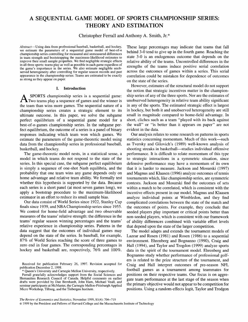
Let j index the game number in the series. Our data consists of seven-games series (j= 1, 2, . . ., 7), but the model applies to any series length n, where n is odd. Figure 1 illustrates the tree for a n = 5 playoff series. A stage of the sequential game is a game in the playoff series. An upward branch from one state indicates that team a won the game and a downward branch indicates team b won the game. Which branch is taken from each state is endogenous and stochastic, with the probability assigned to each branch depending on the relative performance of the teams and on pure luck (i.e., the "bounce of the ball").

The sequential game ends when one team has accumu- lated (n + 1)/2 victories (in figure 1, (5 + 1)/2 = 3). The actual length of the series is therefore endogenous and stochastic, and we denote it n , (n + 1)/2 --- n ' n. Our assumptions will imply that the state of the series, denoted w, is composed of two numbers, (na, nb), where nt is the

number of games already won by team t. Therefore,

w E {(lna' nb): 0 ? max { n, nb(1)

' (n + 1)/2 & O ? n + nb ' nl.

The game number can be recovered from the state, since j =

na + nb + 1. At state w, the strategic choice variable for team t is xt,

interpreted as the team's performance or effort. Since each game is a one-shot stage-game, the strategic decisions made by teams as a game progresses are not modeled. Therefore, xtw captures pre-game strategic decisions, such as which pitcher to start in baseball, and any difficulties related to "psyching up" for a game that depend on its state w. These sports are themselves complicated games with intricate possibilities for changing strategies during the course of the game. It is therefore tempting to try and relate our model to information about the course of play, including the final score, injuries, substitutions, etc. However, our focus is on measuring the impact of strategic considerations generated by the sequential nature of the championship series itself. We therefore limit our attention to variables measurable only at the level of complete games.

The equilibrium choice of x,, is determined by three structural elements of the model:

cost of effort: ctj(x,,,),

score differential: ye = Xa*t, , +Ej, and

final payoff vector:

n* (2)

(Va[na, nbl] - Caj(Xaw), Vb[nb, na]

j=l

n*

- E Cbj(XbW) j=l

FIGURE 1.-TREE DIAGRAM FOR A BEST-OF-FIVE SERIES

(1,O)\ /

(I loy/ )2V

8 \\ / \ + ~~~~~~~~~a Wins

(na,nb)= / /

(0,O)K (1,1)\ (2,2)

\\ / \'+/ 2 b Wins

(0,1)t ~~~~~(1,2) / /

(0,2) 1 2 3 4 5

game number

Note: The pair of numbers is the number of games won by teams a and b coming into the game. An upward arrow indicates the random event that team a wins the game. A downward arrow indicates team b wins the game.

706 THE REVIEW OF ECONOMICS AND STATISTICS

The cost-of-effort function cj;( ) depends implicitly on the rules of the sport and the interaction of players, coaches, and referees. For sports as complicated as baseball, basketball, or hockey, it is not possible to model the equilibrium cost of good performance as a function of the nature of the sport. For instance, if one wished to derive cj1( ) from the "structure" of baseball, it would be necessary to model the sequential decisions made by the manager and players conditional on the score, the inning, the number of outs, the count on the hitter, the quality of the hitter relative to the pitcher and the other hitters in the batting order, and so on. Instead, we exploit the common strategic elements between games of any best-of-n series, taking as given a reduced- form characterization of strategic elements within games. The cost of effort depends upon the state only through the game number j. For instance, ctj may depend upon whether t is playing at home or away.1 The final payoff for team t has two components: the value the team places on the ultimate outcome, denoted Vt[nt, nte], and the total cost of effort expended during the series.

The winner of a game scores more points (or runs or goals). To determine the outcome of a series, the sign of the score difference fully determines the outcome of the game. A single game is therefore a Lazear and Rosen (1981) tournament.2 We require only that the score index ye in equation (2) be a monotonic function of the actual score difference. Linearity of ye with respect to the effort levels is therefore less restrictive than it may appear.

The random term Ej in equation (2) captures elements of luck in the relative performance of the two teams. The luck term is independently and identically distributed across games with distribution and density functions F(Ej) and f(lE), respectively. The probabilities that team a and b win game w, conditional upon their chosen effort levels, can be written

Paw(Xaw,xbw)= Prob (y * > )1 = F( (XawXbw))

-1 - Pbw(Xbw, Xaw)(

The equilibrium level of effort also depends upon the symmetric marginal probability

aPaw(Xaw, Xbw) aPbw(Xbw, Xaw) =f (w f (Xaw Xbw))

= . (4) aXaw aXbw

If the sport were a foot race with several heats, then the model has a simple interpretation (Rosen, 1986). Effort x, is the average speed of racer t in heat w. Racer t wins the heat if his average speed is greater than the speed of his best

competitor, t'. The random term E captures any unforesee- able events, such as cramps, that might occur during the race. A better-conditioned athlete could run any speed x with less effort (lower value of c,,(x)) than a worse athlete. However, the role of conditioning could not be disentangled from psychological factors having to do with competition. Hence, cq, includes the propensity for racer t to "choke" or, alternatively, to "rise to the occasion." In team sports, of course, effort is multidimen- sional. But, in determining the ultimate outcome, effort also aggregates into a single number, the team's score.

AssuMvrION (1).

[1] The abilities of each team in each game, denoted btj, are common knowledge. Cost of effort is exponential in effort and separable in ability:

ctj(x,) = e - tjlrext/r,r (5)

where r > 0 is a constant. [2] The luck distribution F(Ej) is twice continuously

differentiable, symmetric, and has a single peak at Ej = 0: F(Ej) = 1 - F(-Ej); f'(Ej) 0 O for Ej ? 0. Irrelevant games are toss-ups: Pt,(-oo, -oo) = 1/2.

[3] Effort costs are not too convex relative to the density of the luck component: r < l/2f(0).

[4] The luck component is normally distributed: Ej -

N(0, (2).

The negative sign in front of btj in equation (5) implies that larger values of btj are related to higher ability (lower effort costs). In the empirical specification, btj can depend upon observed and unobserved characteristics of team t. The sport-specific parameter r determines the convexity of the cost function. As r tends to zero, the marginal cost of effort below ability btj goes to zero, while the marginal cost of effort above ability goes to infinity. For low values of r, the winning probability (3) in the Nash equilibrium (defined below) will depend on only the invariant ability factors. The case in which teams do not respond to the state of the series is therefore equivalent to a low value of r.

Assumption AL.[2] states that the luck distribution is symmetric around a single peak at Ej = 0. Symmetry implies that the winning probabilities in (3) can be written generically as Pt4(xt, xt ') = F(xt - xt ). If we define

l if t = a it -1 if t= b,

then

F(xt, - xt,) = F(It(xaw - Xbw)), (6)

enabling us to express Pt,(xt, xt ') in terms of the nonge- neric effort levels Xaw and Xbw-

1 This assumption could be relaxed to allow c to depend on other elements of the state of the series. For instance, the idea of "momentum" could be captured by letting c depend upon the winner of the last game.

2 In round-robin tournaments (such as the World Cup of soccer), scores within games do have a direct bearing on the ultimate champion. This means such tournaments are not tournaments in the sense introduced by Lazear and Rosen.


Below it is shown that the value of f(O) determines effort levels in evenly matched games and that condition AL.[3] rules out an equilibrium in which both teams play a mixed strategy.

B. Nash Equilibrium Effort in a Single Game

Nash equilibrium effort of team t in state w maximizes the expected net payoff given the effort of the other team:

max - ctj(xtw) + E[Ptlv(xtw, xtw)AVVt1v]. (7) Xtiv

The expectation in (7) is taken over the distribution of beliefs held by team t concerning effort levels chosen by the other team, xt w. AV, is the value team t places on winning the game and is determined by the Nash equilibrium in subsequent games. Three key indices associated with the state w are

A Vaw incentive advantage: vw In AV'

ability advantage: bj-baj - bbj, and (8)

strategic advantage: Aw rvw + aj

We say that team a has the strategic advantage over team b in state w if the index of strategic advantage is positive, Aw > 0. Otherwise, team b has the advantage. Strategic advantage embodies the net effect of ability advantage by and incentive advantage vw, which in turn incorporates the effect of ability advantages in future games. Proposition 1 demonstrates that zW is indeed a proper measure of strategic advantage. We restrict attention to Nash equilibrium in which teams possi- bly play a mixed strategy consisting of one interior effort level and giving up completely by setting effort to -oo. The equilibrium is described by the effort levels (x4 , x4 ) and the probabilities that teams do not give up, denoted (Yaw,

'Yaw),

PROPOSITION (1).

[1] Under A1.[1]-Al.[2], the Nash equilibrium at any state w of the series satisfies these necessary conditions:

r ln (rYt wf(Aw + r ln -jAVtwe8:tV1)

X* withprob.XA( (9)

-0o

with prob. 1 -

for t E la, b}. Team t plays a pure strategy (ytv = 1) if

0 < -yt'(-rf(A, + r In -yt')

+ F(It/A, + r In -yt',)) + (1 - y)t'w()12.

Otherwise, ywt solves

yt'w [r(Aw + rInY$) +F(w A+rlnY),w] (11)

+ (1- tW) 2 = 0. 2

[2] In equilibrium3

Ptw Prob (team t wins game w)

= PYtW^Yt wF A + r In (12)

(1 + .yW)(l - Yt'iv) +2

2

[3] Let t be the team with a strategic advantage in game j. Under Al.[3], team t chooses greater effort than team ti and follows a pure strategy (ytw = 1). If IAWI is large enough, then team t' gives up with positive probability (t', < 1).

[4] Under Al.[4] the conditions in [1] are sufficient. Otherwise, these conditions may fail to be sufficient when I Aw I is large.

Proof: All proofs are provided in appendix A. Nash equilibrium strategies may not be pure because the

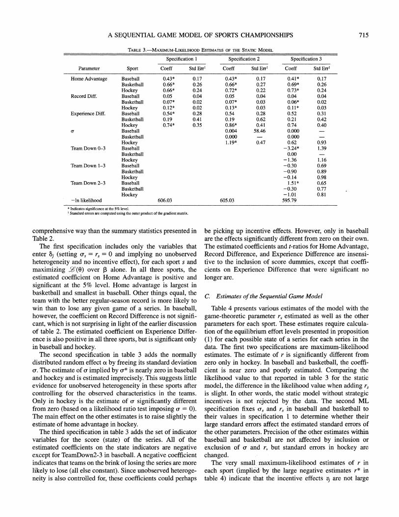
symmetry assumption Al.[2] rules out concavity in the cumulative distribution of the luck factor E. The objective (7) may not be strictly concave so a team may prefer the boundary solution xlw = -oo to the interior solution. If so, the other team would not choose an interior effort level either. Figure 2 illustrates the issue. The components of (7) are shown as a function of team t's effort given an initial value of the other team's effort, xt w, and a luck distribution satisfying Al.[2]. The effort level is so high that for team t the benefit to effort, E[Ptw(xtw, xt,w)AVtw], lies everywhere below the cost, cj(xtw). (Since team t' is playing a pure strategy, the expectation is simply P,(xtV xt w)AVt,.) So team t would choose to give up. As team t' begins to put positive probability on team t giving up, it reduces the marginal value of effort, which lowers xt w. This increases Pt(xt,, xt'w) for every value of xt. The mixed-strategy equilibrium is achieved when the other team's beliefs lead it to set effort to xvw, and the benefit line touches the cost line.

3 P,, is shorthand for PAV(6\V, 'YwVV Yawv)


FIGuRE 2.-MIXED-STRATEGY EQUILIBRIUM

ctj(Xtw)

Ph ( 4w) Xt LAVtw1

E Pt;(xt,,,xtw)AVtI

Xt, w Xt'w xtw

Team t becomes indifferent to giving up and setting effort to some positive value.

Nonconcavity in F also makes it difficult to guarantee that the conditions in proposition (1) are sufficient. Adding the assumption of a normal luck distribution (Al.[4]) provides sufficiency. Even with normality, it is also difficult to rule out the existence of Nash equilibria in which both teams mix over more than one level of interior effort.4

Propositions 1 .[1] also shows that exponential costs imply that AV>, (team t's reward for winning a game) does not determine whether the equilibrium strategy is pure or mixed. The index of strategic advantage, AuW, determines whether either or both teams will follow a pure strategy at state w. A cost function that is not exponential in effort or not separable in ability would generally not lead to such an index, which would make computation of the equilibrium less reliable. Instead, proposition 1.[4] leads to a straightforward algorithm to compute the Nash equilibrium effort levels:

Algorithm for Computing Nash Equilibrium

[NI] Compute Aw. If A%' > 0, then team a will not mix, but team b may. If Aw < 0, then team b will not mix, but team a may.

[N2] Let t be the team that may mix, so yt' = 1. Check condition (10). If (10) is satisfied, then both teams follow pure strategies; i.e., they choose the interior effort levels given in (9). (Done)

[N3] If (10) is not satisfied, then solve the implicit equation (11) for -y,,. Once solved, the interior effort levels of

both teams can also be computed with Yt' = 1. Since the solution to (11) must lie in the range [0,1], a simple bisection method is sufficient to solve for -y>,. (Done)

The algorithm is more robust than one that requires numerical iteration on best response functions. The importance for empirical applications of the model of having such a straightforward and robust algorithm for solving the Nash equilibrium is difficult to appreciate until one considers the number of times this algorithm must be called. The empirical analysis we specify in section IV and then carry out in section V required roughly eight billion solutions to the single-game Nash equilibrium.5

From proposition 1.[4], we can see that whether mixed strategies are every played in equilibrium depends on the parameter r and the absolute value of ability differences A>. We might expect that teams playing in the championship series are relatively evenly matched, since they usually are the two best teams in the league. Both incentive effects and the probability of giving up are small in a championship series compared to, say, a series between the best and worst teams.

C. Subgame Perfect Equilibrium

To derive how strategic incentives evolve during the course of a series, we must specify the value of the final outcomes. We assume that teams behave as if they care only about the ultimate winner of the series and the net costs of effort expended during the series. That is, the final payoff V,(n,, n* - n,) depends only on max nt, n* - ntj, where n*

has been defined as the number of games actually played.6

ASSUMPTION (2). Final payoffs for winning and losing the overall series equal + 1 and -1, respectively. Formally, for tE{ a,bland(n + 1)/2 C n* ?n,

Vt[(n + 1)/2, n* - (n + 1)/2] 1

Vt[n -(n + 1)/2, (n + 1)/2] -1.

PROPOSITION (2).

[1] The subgame perfect equilibrium is defined as the effort functions x4 in (9) and mixing probabilities yt,

4 We have not been able to prove or disprove a claim in an earlier version of this paper that the equilibrium in proposition (1) is unique.

S This approximate figure is calculated from: 16 states X 16 points of heterogeneity X 198 observations X 200 evaluations to maximize the likelihood function X 800 bootstrap resamples = 8,110,080,000. The details of these parts of the estimation process are discussed in section IV.

6 Teams might very well place different values on winning the series. The effect of this difference would, however, not depend upon the state of the series and would act exactly like an unobserved constant in relative ability A>. The empirical analysis controls for unobserved differences in Aj, so setting payoffs equal is simply a normalization.


in (10)-(11), for tE {a, b}, and

Vt[nt, n] ytwVtw [-rf (Aw + r In

YwN + yt'wF fAw + r In -

'Yt'i,v (13) (1 - ytw)

+ 2 [yw VtWV[nt nt, + 1]

+ (1 - y,w)Vt[nt + 1, nt]]

AVtw Vt[nt + 1, nj] - Vt[nt, nt, + 1].

[2] As r - 0, the dynamics within the series disappear, and the outcome of each game only depends on the ability index A>.

Proof: Backwards induction. Proposition 2.[2] implies that the sequential-game model

defined by assumptions (1) and (2) nests an intuitively appealing competing model. As r goes to 0 so does the marginal cost of effort below ability 68. The marginal cost of effort above ability goes to infinity. Therefore, the two teams do not respond to strategic incentives. We call this special case of the subgame perfect equilibrium the static model. In the static model, the outcome of any game depends only upon their relative abilities (including the effect of home advantage). Only factors independent of the state of the series affect relative team performance. Under the static model, many common sports cliches do not apply. For instance, teams do not "play with their backs against the wall" nor do they "taste victory." For large values of r (relative to the ability values), these cliches would apply. They may or may not apply in a given game depending upon how abilities and incentives interact to determine equilibrium effort.

D. Discussion

Before turning attention to the econometric application of the model, we discuss some simulations of the model and some possible extensions.

Table 1 illustrates how the state of the series and the cost parameter r affect winning probabilities in an extended (n = 25) series. (A shorter series is simply the lower-right submatrix.) The series is completely symmetric: ability differences and home advantage are set to 0 (6j = 0 for all j). The left side of the table displays Paw defined in (12) for games in which team a is not leading (n,a ? nb). The right side displays the chances that team a does not give up (Yaw). When the series is even (nal = nb), then Paw = 1/2, and this is emphasized by using a * in the table. If team a's strategic disadvantage is not too large, then 'Yaw = 1, which is also replaced by * in table 1 for emphasis. The luck distribution was assumed to be standard normal, which implies 1/2f(O) = 1.25. This is the upper bound on r in assumption A1.[3] which guarantees that at mnost one team plays a mixed

strategy in equilibrium. The model is then solved with two values of r-one relatively high and one relatively small.

We first note the effect of falling behind in the series. With a high value of r, falling behind just one game has a dramatic effect on equilibrium effort. P,, falls to 0.06 immediately. This is partly due to only a 10% chance that team a tries at all. A large value of r makes equilibrium effort very sensitive to strategic advantage. Falling behind three or four games in a 25 game series leads a team to give up completely.7 Subsequent games have no bearing on the ultimate outcome, so the strategic advantage goes away and both teams put out no effort, leading to equal chances of winning the game (Al.[2]). The state of such a series wanders in the upper-right corner of the table where * appears. If the state approaches the diagonal in the table by team a winning some irrelevant games, then the strategic advantage appears, and team b will again win with probability one.

The second part of table 1 shows equilibrium outcomes for a lower value of r. Winning probabilities are now less sensitive to the state of the series than with a high value of r. Giving up completely happens only in the extremes (the upper corner of the table where team a has fallen hopelessly behind). With a lower r, probabilities differ less away from the main diagonal, but they differ more along bands parallel to the main diagonal than with a high value of r. The strategic effect of being down three games differs a great deal whether there are ten games left or four. For even lower values of r, the probabilities off the diagonal would converge to 1/2, or more generally to the probability associated with 6j in that game.

As noted earlier, our specification of the tournament model allows for heterogeneity in ability and flexibility in the underly- ing elTor distribution while producing a straightforward solution algorithm. There are several other directions one could imagine extending the model. One issue is that luck sometimes spills over into the next game through the effect of injuries. Correlation in E could be adopted by including its expectation conditional upon information available at the start of game j as a state variable. Nonzero expected luck would be equivalent to a change in ability and would not greatly alter the solution algorithm for a single game, but only increase the size of the state space for the sequential equilibrium. A related extension would relax common knowledge of ability (A1.[1]) and allow leaming about relative ability through the outcomes of the series. As long as teams have common, normally distributed prior beliefs about oa, this is again a feasible but computationally burdensome extension.

III. Econometric Specification and Implications

A. Modeling Observed Outcomes of Series

Using proposition (2), the notion that strategic incentives matter can be tested by simply testing whether r is significantly greater than 0. The first step is to posit a specification for the cost of effort parameter ,.

7 This effect is caused by the value of winning the game going to zero in machine precision in the simulation. When the luck factor has a true infinite support, the probability of winning a game in the Nash equilibrium never goes to zero exactly.


TABLE 1 -WINNING PROBABILITIES AND MIXED STRATEGIES IN TWO 25 GAME SERIES (N 25)

Pa,w = Chance team a wins game' NYa = Chance team a tries at all2

nb nb

na 1 2 3 4 5 6 7 8 9 10 11 12 1 2 3 4 5 6 7 8 9 10 11 12

Series I: r = 0.9162, or 73% of 1/@f(0) 0 6% 2% 0% 0% * * * * * * * * 10% 5% 1% 0% * * * * * * * * 1 * 6% 2% 0% 0% * * * * * * * * 10% 5% 1% 0% * * * * * * * 2 * 6% 2% 0% 0% * * * * * * * 10% 5% 1% 0% * * * * * * 3 * 6% 2% 0% 0% * * * * * * 10% 5% 1% 0% * * * * *

4 * 6% 2% 0% 0% * * * * * 10% 5% 1% 0% * * * * 5 * 6% 2% 0% 0% * * * * 10% 5% 1% 0% * * *

6 * 6% 2% 0% 0% * * * 10% 5% 1 % 0% * * 7 * 6% 2% 0% 0% * * 10% 5% 1% 0% *

8 * 6% 2% 0% 0% * 10% 5% 1% 0% 9 * 6% 2% 0% * 10% 5% 1%

10 * 6% 3% * 10% 5% 11 * 7% * 10% 12 * *

Series II: r - 0.3371 or 27% of l/f(0) 0 37% 25% 15% 7% 2% 0% 0% 0% * * * * * * * * * 3% 3% 0% * * * * 1 * 37% 25% 15% 7% 2% 0%O% * * * * * * * * * * 3% 3% * * * * 2 * 37% 25% 15% 7% 2% 0% 0% 0% 0% * * * * * * * 3% 0% 0% 0% * 3 * 37% 25% 15% 7% 2% 0% 0% 0% 0% * * * * * * * 3% 3% 0% 4 * 37% 25% 15% 7% 3% 1% 0% 0% * * * * * * * 3% 3% 5 * 37% 25% 15% 8% 4% 2% 1% * * * * * * * *

6 * 37% 26% 17% 10% 6% 4% * * * * * * * 7 * 38% 28% 19% 13% 9% * * * * * *

8 * 39% 30% 22% 17% * * * * * 9 * 40% 32% 26% * * * *

10 * 42% 34% * * * 11 * 43% * *

12 * *

I * indicates a 50% chance team a will win. 2 * indicates a 100% chance team a will try. Normal distribution of luck which implies that 0.5f(0) = 1.25. Home advantage and ability differences set to zero.

ASSUMPTION (3).

5tj =t + Xtj3, (14)

where Xtj is a vector of observed characteristics of team t in game. j, predetermined at the start of game 1; , is a vector of unknown parameters that determine how strongly a team's ability is predicted by the measurable characteristics Xtj; and at is the residual ability of team t not already captured by Xtj.

In our analysis, Xtj contains the regular-season record, past appearances in the championship series (as a measure of experience), and home or away status in game j. Assump- tion (3) leads to the empirical structure for ability differences and winning probabilities:

observed ability advantage: Xj =Xaj -Xbj, (15)

residual ability advantage: x-= xa ab (16)

net ability advantage: 8j = aj 8 bj = a + Xj;, and

winning probability: Ptw =ytwyt,wF

(Io(t + fX) + rvw)) (17)

+ (1 + ywt)(l -yt, J12

To apply probability (17) to data from an observed series, we must introduce notation to track the sequence of realized states. Let the variable Wj take on the value 1 if team a wins game j of the series, and otherwise Wj equals 0. Let W =

(W1, W2, . . ., W,*) and X = (X1, X2, . . ., Xn*) denote the sequences of outcomes and observable characteristics within a series. Then the realized state in game j is

jl1 j-lI

w(j) -( W., j - n-i W. (18) mn=1 m-1

The probability of the observed sequence of outcomes in a single series is

n*

P*(W, X, 0-; 1, r) J71 [Paw(I)]Wi[ - Paw(j)]1 (19) j=1

PROPOSITION (3).

[1] When P*(W, X, (x; ,, r) is bounded away from 0 and 1, it is a continuous function of the estimated parameters 1B and r.


[2] If the subgame perfect equilibrium consists of pure strategy equilibria at all states of the series, then the equilibrium generates a reduced form that is a panel data binary choice model:

P,,, = F(It(c. + 3Xj + rvw(j)))

+ F(cx + 13XJ + rvw(j))', (20)

X (1 - F(a + Xj + rvw(J)))t.

If Ej is normally distributed, then the reduced form is a probit model with latent regressor rvw(j). If E

follows the logistic distribution, then the reduced form is a logit. If Ej is uniform, then the reduced form is the linear probability model.

[3] In the reduced form, the parameter r is not separately identified.

Proof: Immediate. Continuity of P* in the estimated parameters (3.[1]) is

critical for empirical reasons, and, if attention were paid solely to pure strategies, continuity would not hold. In pure strategies, a small change in the ability index 8i induced by a change in r or an element of 3 could lead to no equilibrium at all, causing the likelihood function to be undefined (or incorrect if the problem were ignored). Maximizing the likelihood function iteratively from arbitrary starting values, even if pure strategies ultimately apply, would be greatly complicated by the discontinuity.

Continuity holds, however, only in series when the winning probabilities remain strictly within the range (0, 1). The simulations in table 1 illustrated this point. When a series reaches a state where y,, = 0, then some other states are not decisive to the ultimate outcome. The winning probability for games that are not decisive reverts to 1/2 (upper-right corners in table 1), because assumption AJ.[2] implies that games that do not matter have equal winning probabilities. A small change in, for example, r can increase yt,' to above zero, making some states decisive again. Their winning probabilities of 1/2 would switch to either very low or very high values. This discontinuity can be avoided by relaxing assumption (A2) and letting the payoffs depend on the number of games won (and not just who won the overall series). Under (A2), winning a game adds nothing to the final payoff unless it changes the probability of winning the overall series. One could allow teams to "play for pride" which would eliminate the possibility that -y, = 0 and the discontinuity caused by meaningless games.

Proposition 3.[2] makes an explicit link between the game-theoretic model and a simpler analysis of game winners using ordinary probit or logit models. That is, define the reduced form of the sequential game model as an analysis based on equation (20) in which the subgame perfect equilibrium is not solved. The reduced form is therefore a binary response model of game winners ex- plained by the vector Xj and unobserved ability difference (x.

The third term of (20), rv>,, is a latent regressor in the reduced form. The incentive advantage vw depends implicitly on r, as well as 1B, a, and the values of Xk, for k > j. Therefore, it is not possible to treat rvW as a typical error term (say, mean zero and heteroskedastic across the state w), because it is correlated with included variables and depends directly on other estimated parameters. Only for a special case of the sequential game model, namely the static r = 0 model, is the reduced form a simple probit-type model with no latent regressor. In this case, the latent term disappears because both of its components go to zero. Hence, neither r nor the value of v, can be recovered from a reduced-form analysis.

In a structural analysis, the subgame perfect equilibrium is solved while estimating the parameters of the model. The incentive advantage v, is no longer free nor unknown, but is instead a computed value associated with each game of all series in the data. Identification of the structural model can be thought of in two steps, although it is more efficient to estimate the model in one step as our bootstrap maximum- likelihood estimator does. First, calculate v, for all games in the data based on initial guesses for r, 1, and the distribution of ax. Then, estimate 1, r, and the distribution of a. using equation (20) as a random-effects probit or logit. Then iterate on these two steps until the values of the parameter estimates in the two stages agree. If equilibrium vw turned out to be proportional to ax/r and ,B/r, then r would cancel out of equation (20) and would not be identified. It is not possible to rule this out analytically, but r does enter the indirect value of each state separately from ax and 13. (See equation (A3) in appendix A.) Therefore, r is potentially identified by outcomes through the structure of the model. Furthermore, r is identified in Monte Carlo experiments we have conducted.

PROPOSITION (4). Let the outcomes of playoff series be generated by the sequential equilibrium. Then estimates of P are inconsistent if the sequential equilibrium is not solved. The amount of bias increases with the cost of effort parameter r, holding all else constant.

One might try to avoid proposition (4) by approximating the incentive effect with dummy variables for the current state of the series:

rvWv(j) -3 I*(wj), (21)

where I* is a vector with elements contained in{- 1, 0, 1} that depend on the state of the series.8 The vector 13 would be estimated state-of-the-series effects. The problem with approximation (21) is that the strength of the incentive index v,(j) depends on the relative strength of the teams in the

8 We estimate exactly this approximation in the next section. Taylor and Trogdon (1999) use this approach to study the effect of the NBA draft lottery.


current and all subsequent games, IXk, k = j, j + 1, . . . , n. The error in using (21) to approximate vw(j) is therefore correlated with the other regressors. Estimates of 3 are still biased even with a large sample of series.9

We assume the residual ability index at follows the normal distribution across series, at - N(0, u2), for oU2 > 0. Under assumption Al. [1], the value of at is common knowledge of the two teams. Given their information, the probability of a series of outcomes W is P*(W, X, ax; 3, r), defined in equation (19). To the econometrician, however, the probability is

Q(W, X; , , r) (22)

- (P(W, X, oa; , r)4(oal)Iudoa.

Assuming falsely that a2 =0 (no unobserved heterogeneity) induces correlation between winning probabilities of different games conditional upon the observed ability factors.

In a panel-data model, correlation caused by unobserved heterogeneity leads to inconsistent estimates of P. For example, we observe in the sports data that, when teams are down 3-0, they usually lose the fourth game and conse- quently the series. This may be because teams down 3-0 give up in the situation (i.e., vu, is large in absolute value), or because outmatched teams are more likely to reach the situation (i.e., at is large in absolute value), or both. The first reason is true state dependence while the second is spurious and due simply to ability differences making it likely that a series that reaches the state 3-0 has unevenly matched teams.

B. Adding Covariates for Ability

The team that played at home in game 1 is coded as the reference team (team a in the model section). For example, the endogenous variable Wjis takes on the value 1 if the team that played at home in game 1 wins game j of the series i in sport s, and otherwise Wjis equals 0. Three measures of relative team ability were also collected: an indicator for home advantage in game j (Home Advantageijs), difference in regular season records (Record Diffis), and an indicator for differences in appearance in last year's championship series (Experience Diffis). The latter two variables do not vary with game number j. (These and other variables derived from the data are defined in appendix B.)

Our random-effects estimation procedure controls for both true state dependence created by incentive advantages, and serial correlation created by unobserved heterogeneity.

The complete specification of the structural parameters of the game-theoretic model is

8 ij = oti + pxij

C=i + r3Home Advantageij1

+ P3 'Record Diffi

+ P3Experience Diffai (23) 1* r= els

eE

F(E) = 1 + ee

Superscripts have been added to Pk and subscripts have been added to r and oa to indicate that these values are estimated separately for each sport s. We estimate r* and a* to avoid having a closed lower bound on the parameter space. Large negative values of r* and a* therefore correspond to values of rs and as near 0. The luck factor follows the standard logistic distribution. All estimated values are therefore relative to the variance of random luck inherent in the sport. Based on equations (22) and (23), let Qi5(Wis, Xis; os, Ps, rs) denote the predicted probability of the i-th series in sport s, where superscripts have been added to the data vectors W and X. Denote the vector of estimated parameters as 0 (that is, the concatenation of Ps, r*, and o* for all three sports). The log likelihood function for the combined sample is

Y(O)- I n Qis(Wisg X is; 98 PS r s*. (24) s i

Each championship series is, in effect, a short panel of observations. While maximum-likelihood estimates are consistent in this context, they may not perform well in samples of the size available here.10 One way to correct for this type of small sample problem is to perform bootstrap estimation. The sample data is randomly sampled with replacement to form artificial data sets of the same size.11 Let the ML estimate from the actual sample be OML. ML estimates of 0 are also obtained for each artificial data set. With the average estimated vector across resamples denoted 6, the parametric bootstrap estimate is defined (Efron & Tibshirani, 1993, ch. 10)as

0BS = 20ML - 0 (25)

9 Interacting the indicator vector with the observable ability vector X reduces the bias but does not guarantee that approximation error is eliminated. For example, the incentive component in one game not only depends on which team has the home advantage in this game, but also the sequence of future home advantages. Given the fixed maximum-panel length of 7, including interaction terms may make the bias in estimating 3 worse by including extra parameters.

10 We conducted Monte Carlo experiments on the ML estimates of the sequential equilibrium model. Not surprisingly, we found significant bias in the ML estimates with small samples and short series. There was a strong tendency for estimates of r, to be pushed close to zero when the true values was greater than zero.

11 Each series represents an observation to be sampled, not individual games within series.


C. Application to Firms

The tournament models of Lazear and Rosen (1981) and Rosen (1986) were designed to explain wage and promotion patterns within firms. Our version of the model provides no further insight into firms, but its straightforward solution algorithm in the presence of heterogeneity in ability makes it a potentially useful tool for empirical studies of wages within firms.

To build a model of the firm, the connection between effort levels and output would be specified, so that the firm would care about the effort levels generated through competition for higher-wage positions. The firm would take as given the distribution of ability. The firm would control effort by setting the wage levels (or final payoffs) and the length of the competition, which would relate to the expected time between promotions. The model could easily be adapted to a situation in which the series length is not fixed but instead ends with some probability and the player who is ahead at that point wins. At the same time, the firm's internal wage policies would be subject to a participation constraint. The screening element of promotion competition (placing more able people in critical jobs) could also be included by modeling multistage tournaments. As in Rosen (1986), this requires additional assumptions about the beliefs held over the ability of opponents in future rounds. By solving the firm's problem numerically and relating its predictions to observed wages and career profiles, the effect of competition and incentives within the firm could be inferred. Although there are many theoretical and econometric issues related to such a project, our robust and flexible model of competition itself removes one of the key stum- bling blocks.

IV. Empirical Analysis

A. Data

The data consist of championship series in professional baseball (Major League Baseball), professional ice hockey (National Hockey League), and professional basketball (National Basketball Association). Major rule changes over the course of the last century created the modem versions of each of the sports. In each sport, we selected our sample period to include all best-of-seven series since the introduction of these rule changes. Baseball introduced the "live ball" in 1920, but the 1920 and 1921 World Series were nine-games series, so the baseball sample covers 1922- 1993.12 Professional basketball introduced the 24-second clock in the 1954-1955 season, so the basketball sample covers 1955-1994. Finally, hockey introduced icing in the 1937-1938 series, but the 1938 Stanley Cup was a five-game series, so the hockey sample covers 1939-1994.

Table 2 reports summary statistics for each sport. The distribution of series length (n*) is an endogenous aspect of

the model, reflecting both ability differences and incentive effects. Baseball series are on average the longest: 42% of the 72 series go to 7 games, whereas 30% of the 40 basketball series, and only 18% of the 56 hockey series go to 7 games. Four-game series occur infrequently in both basketball (13% of the series) and baseball (18% of the series). By contrast, 29% of the series end in four games in hockey, the most frequent series length. Basketball and hockey shared the same sequence of home advantage until 1985, when basketball switched to the sequence used in baseball.

Our empirical specification includes two fixed measures of relative team ability-the difference between regular season records and experience in the previous championship series. The average absolute difference in records (across series not games played) is smallest in baseball and largest in

TABLE 2.-SUMMARY OF CHAMPIONSHIP SERIES AND GAMES

Baseball Basketball Hockey World Series NBA Finals Stanley Cup

1922-93 1955-94 1939-94

Series

Total 72 40 56 % Ending After

4 Games 18 13 29 5 Games 21 23 27 6 Games 19 35 27 7 Games 42 30 18

Home Sequence HHAAAHH' HHAAHAH2 HHAAHAH HHAAAHH3

Mean Abs (record difference) 4.04 10.32 9.77

% With experience difference 47 38 50

% Won by the team with better season record 53 68* 79* experience advantage 68* 73* 64*

Mean (st. dev.) of model variables

Total games played 421 233 299 W (1 = Team a won, 0.553 0.588 .0.609

0 = Team a lost) (0.50) (0.49) (0.49) Home Advantage (+ 1/-1) 0.002 0.073 0.084

(1.00) (1.00) (1.00)

Record Difference 1.004 9.953 8.121 (4.52) (8.17) (8.46)

Experience Difference 0.216 0.172 0.151 (+ 1/0/- 1) (0.60) (0.60) (0.67)

Team Down 0-3 -0.012 -0.013 -0.023 (+ 1/0/- 1) (0.19) (0.15) (0.26)

Team Down 1-3 -0.024 -0.034 -0.023 (+ 1/0/- 1) (0.26) (0.26) (0.29)

Team Down 2-3 0.000 -0.026 -0.030 (+ 1/0/- 1) (0.32) (0.33) (0.29)

% of games won by team with Home Advantage 56* 60* 58* 1-0 Lead 47 42 67* 2-0 Lead 44 29* 58 3-0 Lead 87* 100* 76* 2-1 Lead 46 46 57 3-1 Lead 54 56 60 3-2 Lead 32* 54 60

Sources: The Baseball Encyclopedia, Macmillan; The Sports Encyclopedia: Pro Basketball, St. Martin's; The National Hockey League Official Guide and Record Book, Triumph.

I Other sequences were used in 1923, 1943-44, and 1961. 2 Sequence used until 1985. 3 Sequence used after 1985. * = different from 50% given the number of games/series at a 10% level of significance.

12 The 1994 World Series and 1995 Stanley Cup were not played due to strikes by the players.


basketball. The sports are similar in terms of the number of series where one team has an experience advantage: half of the hockey series, 47% of the baseball series, and 38% of the basketball series.

These measures of ability are generally related to which team wins the overall series. The team with either advantage (not controlling for other factors) wins the overall series more often. The proportion does not differ significantly from 50% in baseball when looking at the difference in season records. This compounds two differences between baseball and the other sports that suggest that relative record differences will be less correlated with relative playing ability in baseball. One is simply that the average record difference is smaller in baseball. The other is how the baseball regular season itself was organized during the sample period. Until 1997, the two teams meeting in the World Series came from leagues that did not play each other during the regular season. The difference in their respective champions' regular season records would therefore contain less information about the teams' relative ability than the records of teams in the basketball and hockey championships that played many common opponents.

The second part of table 2 summarizes the variables used in the empirical analysis using individual games as the sampling unit. (Complete definitions are given in appendix B.) The baseball sample includes 421 games, the basketball sample includes 233 games, and the hockey sample includes 299. Recall that the team that played at home in game 1 is coded as the reference team (team a), so W equals 1 whenever that team wins a game. The average value of W being above 0.50 in each sport reflects the fact that the team that plays at home in the first game wins more games overall. The positive average value of the home-advantage indicator indicates that team a also plays more games at home. The greater values in basketball and hockey reflect in part their sequence of home advantage in which team b never plays more games at home than team a. In baseball and the last part of the basketball sample, however, team b plays more games at home for series that end in five games.

The pattern across sports in the regular-season record differences reflects both the wider range of values in baseball and hockey and the different ways in which it is decided who plays at home first. Baseball would also tend to have lower variation in record differences, because it has always had a much shorter playoff structure. This makes it impossible to get into the World Series with a poor regular-season record; whereas, in basketball and hockey, teams that finished well behind in the regular season could end up in the championship series.

The TeamDown variables are indicators for certain values of the state vector wj following the definition given in equation (21). Including these variables in a reduced-form model is an ad hoc way to control for the incentive advantage. For example, TeamDownO-3 is defined to be 0 except for fourth games where the state is (0, 3) or (3, 0), in which case it takes on the values + 1 and -1, respectively.

TeamDownl-3 and TeamDown2-3 are defined similarly. The negative mean values for these variables indicate that team a reaches the brink of defeat less often than team b. In baseball, there are exactly equal numbers of series in which the teams end up down 2-3.

The bottom of table 2 shows the sample proportion of victories in the current game conditional upon various aspects the current state of the series. Note that victory in this case is not consistently defined in terms of team a or b, but rather for whichever team is in the given situation. For example, in all three sports, the team playing at home is significantly more likely to win the game. The other statistics show the conditional probability that the team leading in the series wins the current game. These values can be misleading, because they mix the effect of fixed ability differences between the teams (better teams tending to lead the series) and state-dependent incentive effects (teams giving up when they fall behind as illustrated in the simulations in table 1). They also mask the patterns of home advantage in the different sports. For example, teams leading 2-0 are more likely to lose the third game in baseball and basketball (with the difference statistically significant in basketball). But it is often the case that this team is now playing away for the first time in the series, so this apparent state effect may simply reflect a strong effect of home advantage in basketball. Interestingly, in hockey, the leading team is always more likely to win the current game, although the difference is insignificant in several cases. Since the unconditional home advantage is about as strong in hockey, this pattern suggests either larger ability differences or larger incentive effects in hockey (or both).

In all three sports, teams leading 3-0 or 3-1 are more likely to win the game and end the series. In basketball and hockey, the same is true for teams ahead 3-2, but the effect is not statistically significant. In baseball, however, the team behind is more likely to win the sixth game and force a seventh game. This can also be seen simply from the distribution of series length shown in table 2, because baseball has more seven-game series than six-game series.

Although these statistics that condition on the state of the series suggest that the state may be an important factor in determining the winner of the current game, it is difficult to draw any strong conclusions without controlling simulta- neously for home advantage, observed and unobserved differences in the strengths of the teams, and the possible incentive effects induced by the current state of the series.

B. Estimates of the Static Model

Table 3 reports logit estimates of the winner of games in each sport.13 The specifications correspond to the static r ) 0 model (equivalent to r* -oo). Since these are simple logit estimates, the results also summarize the patterns in the data that the dynamic model seeks to explain in a more

13 We also estimated the model assuming a normal distribution (with the same variance as the standard logistic). The results were nearly identical.


TABLE 3.-MAXIMUM-LIKELIHOOD ESTIMATES OF THE STATIC MODEL

Specification 1 Specification 2 Specification 3

Parameter Sport Coeff Std Errf Coeff Std Err1 Coeff Std Err'

Home Advantage Baseball 0.43* 0.17 0.43* 0.17 0.41* 0.17 Basketball 0.66* 0.26 0.66* 0.27 0.69* 0.26 Hockey 0.66* 0.24 0.72* 0.22 0.73* 0.24

Record Diff. Baseball 0.05 0.04 0.05 0.04 0.04 0.04 Basketball 0.07* 0.02 0.07* 0.03 0.06* 0.02 Hockey 0.12* 0.02 0.13* 0.03 0.11* 0.03

Experience Diff. Baseball 0.54* 0.28 0.54 0.28 0.52 0.31 Basketball 0.19 0.41 0.19 0.62 0.21 0.42 Hockey 0.74* 0.35 0.86* 0.41 0.74 0.40 Baseball 0.004 58.46 0.000 Basketball 0.000 0.000 Hockey 1.19* 0.47 0.62 0.93

Team Down 0-3 Baseball -3.24* 1.39 Basketball 0.00 Hockey -1.36 1.16

Team Down 1-3 Baseball -0.30 0.69 Basketball -0.90 0.89 Hockey -0.14 0.98

Team Down 2-3 Baseball 1.51* 0.65 Basketball -0.30 0.77 Hockey -1.01 0.81

-ln likelihood 606.03 605.03 595.79 * Indicates significance at the 5% level,

Standard errors are computed using the outer product of the gradient matrix.

comprehensive way than the summary statistics presented in Table 2.

The first specification includes only the variables that enter 6j (setting a, = r= 0 and implying no unobserved heterogeneity and no incentive effect), for each sport s and maximizing S(O) over , alone. In all three sports, the estimated coefficient on Home Advantage is positive and significant at the 5% level. Home advantage is largest in basketball and smallest in baseball. Other things equal, the team with the better regular-season record is more likely to win than to lose any given game of a series. In baseball, however, the coefficient on Record Difference is not significant, which is not surprising in light of the earlier discussion of table 2. The estimated coefficient on Experience Differ- ence is also positive in all three sports, but is significant only in baseball and hockey.

The second specification in table 3 adds the normally distributed random effect ox by freeing its standard deviation u. The estimate of c implied by u* is nearly zero in baseball and hockey and is estimated imprecisely. This suggests little evidence for unobserved heterogeneity in these sports after controlling for the observed characteristics in the teams. Only in hockey is the estimate of u significantly different from zero (based on a likelihood ratio test imposing u = 0). The main effect on the other estimates is to raise slightly the estimate of home advantage in hockey.

The third specification in table 3 adds the set of indicator variables for the score (state) of the series. All of the estimated coefficients on the state indicators are negative except for TeamDown2-3 in baseball. A negative coefficient indicates that teams on the brink of losing the series are more likely to lose (all else constant). Since unobserved heterogeneity is also controlled for, these coefficients could perhaps

be picking up incentive effects. However, only in baseball are the effects significantly different from zero on their own. The estimated coefficients and t-ratios for Home Advantage, Record Difference, and Experience Difference are insensi- tive to the inclusion of score dummies, except that coefficients on Experience Difference that were significant no longer are.

C. Estimates of the Sequential Game Model

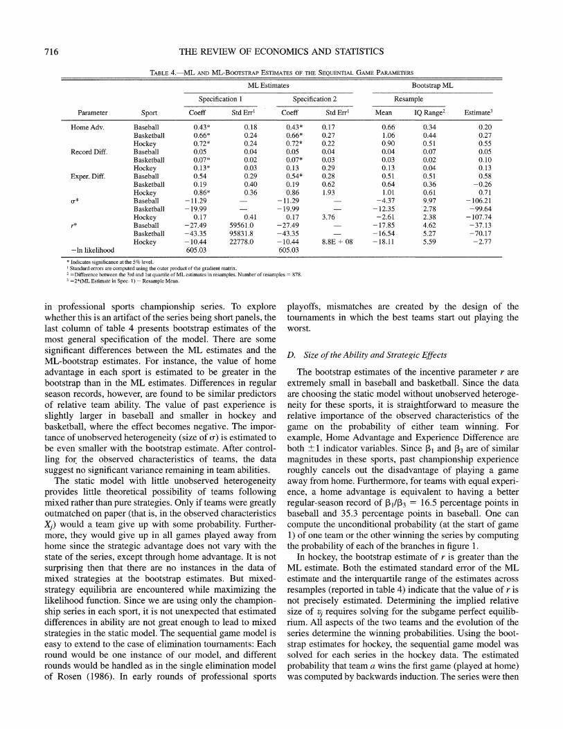
Table 4 presents various estimates of the model with the game-theoretic parameter rs estimated as well as the other parameters for each sport. These estimates require calcula- tion of the equilibrium effort levels presented in proposition (1) for each possible state of a series for each series in the data. The first two specifications are maximum-likelihood estimates. The estimate of r is significantly different from zero only in hockey. In baseball and basketball, the coefficient is near zero and poorly estimated. Comparing the likelihood value to that reported in table 3 for the static model, the difference in the likelihood value when adding rs is slight. In other words, the static model without strategic incentives is not rejected by the data. The second ML specification fixes u, and r, in baseball and basketball to their values in specification 1 to determine whether their large standard errors affect the estimated standard errors of the other parameters. Precision of the other estimates within baseball and basketball are not affected by inclusion or exclusion of u and r, but standard errors in hockey are changed.

The very small maximum-likelihood estimates of r in each sport (implied- by the large negative estimates r* in table 4) indicate that the incentive effects vj are not large


TABLE 4.-ML AND ML-BOOTSTRAP ESTIMATES OF THE SEQUENTIAL GAME PARAMETERS

ML Estimates Bootstrap ML

Specification 1 Specification 2 Resample

Parameter Sport Coeff Std Err' Coeff Std Err' Mean IQ Range2 Estimate3

Home Adv. Baseball 0.43* 0.18 0.43* 0.17 0.66 0.34 0.20 Basketball 0.66* 0.24 0.66* 0.27 1.06 0.44 0.27 Hockey 0.72* 0.24 0.72* 0.22 0.90 0.51 0.55

Record Diff. Baseball 0.05 0.04 0.05 0.04 0.04 0.07 0.05 Basketball 0.07* 0.02 0.07* 0.03 0.03 0.02 0.10 Hockey 0.13* 0.03 0.13 0.29 0.13 0.04 0.13

Exper. Diff. Baseball 0.54 0.29 0.54* 0.28 0.51 0.51 0.58 Basketball 0.19 0.40 0.19 0.62 0.64 0.36 -0.26 Hockey 0.86* 0.36 0.86 1.93 1.01 0.61 0.71 Baseball -11.29 -11.29 -4.37 9.97 -106.21 Basketball -19.99 -19.99 -12.35 2.78 -99.64 Hockey 0.17 0.41 0.17 3.76 -2.61 2.38 -107.74

r* Baseball -27.49 59561.0 -27.49 -17.85 4.62 -37.13 Basketball -43.35 95831.8 -43.35 -16.54 5.27 -70.17 Hockey -10.44 22778.0 -10.44 8.8E + 08 -18.11 5.59 -2.77

-ln likelihood 605.03 605.03 * Indicates significance at the 5% level.

Standard errors are computed using the outer product of thie gradient matrix. 2 =Difference between the 3rd and 1st quartile of ML estimates in resamples. Number of resamples = 878. 3 =2*(ML Estimate in Spec. 1) - Resample Mean.

in professional sports championship series. To explore whether this is an artifact of the series being short panels, the last column of table 4 presents bootstrap estimates of the most general specification of the model. There are some significant differences between the ML estimates and the ML-bootstrap estimates. For instance, the value of home advantage in each sport is estimated to be greater in the bootstrap than in the ML estimates. Differences in regular season records, however, are found to be similar predictors of relative team ability. The value of past experience is slightly larger in baseball and smaller in hockey and basketball, where the effect becomes negative. The importance of unobserved heterogeneity (size of u) is estimated to be even smaller with the bootstrap estimate. After controlling for the observed characteristics of teams, the data suggest no significant variance remaining in team abilities.

The static model with little unobserved heterogeneity provides little theoretical possibility of teams following mixed rather than pure strategies. Only if teams were greatly outmatched on paper (that is, in the observed characteristics Xj) would a team give up with some probability. Further- more, they would give up in all games played away from home since the strategic advantage does not vary with the state of the series, except through home advantage. It is not surprising then that there are no instances in the data of mixed strategies at the bootstrap estimates. But mixed- strategy equilibria are encountered while maximizing the likelihood function. Since we are using only the championship series in each sport, it is not unexpected that estimated differences in ability are not great enough to lead to mixed strategies in the static model. The sequential game model is easy to extend to the case of elimination tournaments: Each round would be one instance of our model, and different rounds would be handled as in the single elimination model of Rosen (1986). In early rounds of professional sports

playoffs, mismatches are created by the design of the toumaments in which the best teams start out playing the worst.

D. Size of the Ability and Strategic Effects

The bootstrap estimates of the incentive parameter r are extremely small in baseball and basketball. Since the data are choosing the static model without unobserved heterogeneity for these sports, it is straightforward to measure the relative importance of the observed characteristics of the game on the probability of either team winning. For example, Home Advantage and Experience Difference are both 1+ indicator variables. Since PI and r3 are of similar magnitudes in these sports, past championship experience roughly cancels out the disadvantage of playing a game away from home. Furthermore, for teams with equal experience, a home advantage is equivalent to having a better regular-season record of 11/03 = 16.5 percentage points in baseball and 35.3 percentage points in baseball. One can compute the unconditional probability (at the start of game 1) of one team or the other winning the series by computing the probability of each of the branches in figure 1.

In hockey, the bootstrap estimate of r is greater than the ML estimate. Both the estimated standard error of the ML estimate and the interquartile range of the estimates across resamples (reported in table 4) indicate that the value of r is not precisely estimated. Determining the implied relative size of vj requires solving for the subgame perfect equilibrium. All aspects of the two teams and the evolution of the series determine the winning probabilities. Using the bootstrap estimates for hockey, the sequential game model was solved for each series in the hockey data. The estimated probability that team a wins the first game (played at home) was computed by backwards induction. The series were then


TABLE 5.-DISTRIBUTION OF WINNING PROBABILITIES IN HocKEY1

Pa<, = Chance team a wins game nb

na 0 1 2 3

25th Percentile: A(o,o) = 0.96 0 0.622 0.621 0.472 0.472 1 0.622 0.473 0.473 0.621 2 0.474 0.473 0.622 0.472 3 0.474 0.622 0.473 0.621

50th Percentile: A(g,o) = 1.68 0 0.714 0.714 0.576 0.575 1 0.714 0.577 0.576 0.713 2 0.578 0.577 0.714 0.576 3 0.578 0.714 0.577 0.714

75th Percentile: A(g,o) = 2.50 0 0.796 0.795 0.679 0.678 1 0.796 0.680 0.679 0.794 2 0.680 0.680 0.795 0.679 3 0.681 0.796 0.679 0.795

XEstimated probabilities that the hockey team playing at home in game 1 (team a) wins the game based on the simulated distribution of A(o,o) using the bootstrap estimates in table 4 and the sample distribution of X variables. From this distribution, the series at the respective percentiles were selected.

Boldface indicates team a would be playing away.

ranked in order of this initial probability (or, equivalently, by the order of the strategic advantage in game 1, A(g,o)). The series at the 25th, 50th, and 75th percentiles were found. For these three series, the probability of team a winning in each state of the series is shown in table 5. For example, the home team at the 25th percentile wins the first game with probability 0.622. This indicates that "home ice" gives team a an edge in game 1 even when though its observable characteristics put it in the bottom quarter of the game 1 winning probabilities.

The difference in probabilities across the empirical distribution of abilities is large. The ratio of probabilities between the 75th and 25th percentiles is 1.28: A superior team is 28% more likely to win the first game at home than an inferior team. The percentage change when playing at home ranges from 31% at the 25th percentile to 17% at the 75th percentile.

In contrast, the effect of the state of the series is negligible. This can be read from table 5 by tracing probabilities along the minor diagonals (which holds constant the game number). For example, game 6 can have either the state (3, 2) or (2, 3). In the series at the 75th percentile in initial advantage, the ratio of the two probabilities of team a winning is only 0.6794/0.6787 = 1.001. The upshot is that the bootstrap estimate of r in hockey, while much larger than in the other sports, is still too small to generate any significant incentive effects in the series. The effect of home advantage and constant-ability differences swamp any strategic effects generated by the sequential nature of the playoff series.

V. Conclusion

This paper has analyzed outcomes in professional sports championship series to explore some empirical implications of game theory. We have developed a sequential game model

of best-of-n-games series and have estimated the model's parameters using data from three professional sports. We estimate the effect of home advantage and differences in relative team ability revealed by differences in regular- season records and previous appearances in the championship series. We use a bootstrap procedure to improve the small-sample properties of the maximum-likelihood estimator. We control for unobserved differences in relative team abilities as well as the strategic effects on performance arising from the subgame perfect equilibrium of the sequential game. The strength of the strategic effect is determined by a single estimated parameter. We find no evidence of strategic effects in the data for any of the three sports. Only in hockey do the magnitude and imprecision of the estimates leave open the possibility of a measurable strategic effect, but the effect on winning probabilities at the bootstrap estimates is negligible when compared to, say, the effect of home advantage. We conclude that a simple model in which teams do not give up nor get overconfident based -on the outcome of previous games in the series best explains the outcomes of championship series. We also find that unobserved heterogeneity in ability differences is not helpful in explaining the data after controlling for regular-season records and previous championship experiences. That is, teams are estimated to be just as good as they appear on paper.

Why are there no incentive effects? One possibility is that strategic interactions within games cancel out any incentive effects between games of a series. For example, team behavior may act to focus individual players on winning the current game and to ignore the larger sequential nature of the playoff series, even when winning or losing the game is nearly meaningless. Perhaps a cooperative model of teammates might explain what elements of the sport would enable this outcome to occur. Such a theoretical exercise would attempt to make our primitive parameter r an endogenous function of the sport. Also, it may be that players in these series are in some sense immune to these incentives. Perhaps players who reach the highest championship in the sport do indeed play to the best of their ability regardless of the circumstances.

Two other sports applications of the model are possible. First, the model can be estimated on several rounds of single-elimination tournaments that lead to championship series, either in these sports or other sports. In earlier rounds, the differences in abilities in the teams tend to be much greater. Larger differences in ability also lead to a greater likelihood of teams giving up. This suggests that any teammate interaction that mitigates strategic incentives would become less effective in earlier rounds.

Another application is to perform the same estimation procedure on tennis matches. Each game of a tennis match is similar to a championship series, except the game does not end when one player scores (n + 1)/2 points, because a tennis game has no maximum number of points n. Instead, the game winner is the player that scores four or more points


and leads by at least two points. Each set is, in turn, similar to a championship series, but one that relies on a cost function specified for each point rather than each game. Furthermore, strategic advantage rises and falls within a tennis match because the first point of a new game is less decisive to the ultimate outcome than the game point in the previous game. Compared to a simple championship series between teams, a tennis match between individuals may provide more leverage to identify strategic incentives.

While sports is a natural arena for testing the tournament model, the model was developed by Lazear and Rosen (1981) to study wages within firms that have workers compete for fixed-valued prizes, such as promotions or bonuses. However, there have been few direct tests of the tournament model as an explanation for wages and promotion polices within firms. The specific tournament model developed here provides a robust computational framework for studying empirically any contest between heterogeneous players composed of a sequence of identical stage games. It may therefore serve as a basis for further empirical work outside of sports.

REFERENCES

Craig, L. A., and A. R. Hall, "Trying Out for the Team: Do Exhibitions Matter? Evidence from the National Football League," Journal of the American Statistical Association 89 (Sept., 1994), 1091-1099.

Efron, B., and R. J. Tibshirani, Introduction to the Bootstrap (New York: Chapman and Hall, 1993).

Ehrenberg, R. G., and M. L. Bognanno, "Do Tournaments Have Incentive Effects," Journal of Political Economy 98 (Dec., 1990), 1307- 1324.

Jackson, D., and K. Mosurski, "Heavy Defeats in Tennis: Psychological Momentum or Random Effect," Chance 9 (Spring, 1997), 27-34.

Lazear, E. P., "Pay Equality and Industrial Politics," Journal of Political Economy 97 (June, 1989), 561-580.

Lazear, E. P., and S. Rosen, "Rank-Order Tournaments as Optimal Labor Contracts," Journal of Political Economy 89 (Oct., 1981), 841- 864.

Magnus; J., and F. Klaasen, "Testing some Common Tennis Hypotheses: Four Years at Wimbledon," manuscript, Center for Economic Research, Tilburg University (1996).

Rosen, S., "Prizes and Incentives in Elimination Tournaments." American Economic Review 76 (Sept., 1986), 701-715.

Taylor, B. A., and J. B. Trogdon, "Losing to Win: Tournament Incentives in the National Basketball Association," manuscript, Baylor Univer- sity (1999).

Tversky, A., and T. Gilovich, "The Cold Facts about the 'Hot Hand' in Basketball," Chance 2 (Winter, 1989), 16-21.

APPENDIX A: PROOF OF PROPOSITIONS

A.1 Proposition (1)

Proposition 1[1] and 1.[2].

Step 1. Given that team t' is choosing a mixed strategy of the form (9), the objective of team t in choosing effort takes the form

-e-'-I,erX>, + yt'wF(lt(xaw - XbW))AVt. (Al)

+ (1 - yt,J)Vt(nt + 1, nt,) + ytV, Vt(nt, nt,+).

Necessary conditions for an interior solution for teams a and b are the first-order conditions

exatir = rybf(Xa- xbw)AVawe a/ (A2.1)

exbIr = rYawf (Xaw -XbW)AVbwebi/. (A2.2)

After some manipulation, their ratio leads to

Ybw Xaw-Xbw.= Av + r ln-. (A3)

,yaw

Replacing (A3) in the first-order conditions leads to the interior effort levels in (9).

Step 2. Substituting the interior effort level (9) into (7) leads to the indirect value of the interior solution as a pure strategy for team t:

yt,w AVt(-rf(Aw + r ln y t w) + F(ItAw + r ln -yt w)) (A4)

+ (1 - y,w)Vt(nt + 1, nt) + ytwVt(nt, nt + 1).

If team t gives up and sets x, = -oo and team t' puts in any effort at all, then t loses the game with certainty. Team t' puts in effort with probability y,,t. A1.[2] handles the case in which they both give up, so the indirect value to team t of giving up at state w is

Vt(nt + 1, nt) + Vt(nt, nt' + 1) ,ytwwVt(nt, nlt + 1) + (1 - jYtw) 2 ' (A5)

Comparing (A4) and (A5), the interior solution is weakly preferred to giving up if

AVt, [jt,w(-7rf(Aw + r In iYt,w)

+ F(ItAw + r In Yt'w)) + (1 - Yt'w) - 0.

Dividing by AV,,v leads to the condition (10). If the inequality in (10) holds strictly, then team t prefers the pure strategy and sets yt, = 1 in equilibrium.

Step 3. If (10) does not hold, then team t prefers the boundary solution and team t' would not follow the first-order condition. A value of -Ytw less than 1 induces team t' to lower its effort level in the interior solution. At the Nash equilibrium in mixed strategies, team t is indifferent between giving up and the interior solution, so (11) holds with equality.

Step 4. Substituting the interior effort levels into (6) and taking into account the probabilities of giving up lead to (12). QED

PROPOSITION 1.[3] Suppose the teams are equally matched (Aw = 0). Then, under A1.[2],

F(Aw) = 1/2, and effort will be symmetric. Looking at (10), equally matched teams choose pure strategies if Al. [3] holds. In an even match, the sign of the luck factor E determines the winner, andf(0) determines effort levels on the margin. As long as costs are not too convex relative tof(0), evenly matched teams strictly prefer the interior solution and will not play mix strategies. (Rosen (1986) recognized condition A1.[3] within a model of promotion ladders but focussed the analysis on pure strategy equilibria.) When IA, > 0, assumption AL1[2] implies -rf(Aw) + F(ItAw) > -rf(0) + - > 0. So team t puts no probability on giving up. If IAwI is near zero, then the team behind is close enough not to give up completely but simply put in less effort. Only when |Aw I gets large enough will the team at a strategic disadvantage give up with positive probability. When the team behind gives up with positive probability, the effort differential is reduced by -r ln -yt,. This effect is bounded by I AwI in equilibrium, so the team with the strategic advantage always sets higher interior effort. (Otherwise, the net advantage would become nonpositive, and the team behind would stop giving up by setting yt, = 1.) Since the team with strategic advantage sets higher interior effort and never gives up, the first part of proposition 1.[3] follows as well. QED


PROPOSITION 1.[4] Under a normal luck distribution (A1.[4]), the first-order condition for

team t takes the form

12 2 ex= ryt,we(-(-Xwxb,,)2)/29, i\V 9ebi/r (A6)

2~ro

The right-hand side of (A6) lies below the marginal cost of effort function as xt, goes to -co (because the quadratic term converges to zero more quickly than the left-hand side). Taking the logarithm of both sides leads to a quadratic equation in x, with at most two real solutions. If there is zero or one real solution, then the team prefers to give up with probability one and would not be part of a Nash equilibrium. If there are two solutions, then the larger solution for xt, is the only interior local maximum. The conditions in proposition (1) guarantee that it is a global maximum. So, the necessary conditions for a Nash equilibrium are also sufficient. QED

Without assuming A1.[4] but still assuming A1.[2], the second-order condition for the interior solution can be written

r2 yt,wsgn(xt - xt'w)f'( Xaw - XbWl)LVtw < e-8tj/rextnJr, (A7)

where sgn(x) is the sign of x. This condition holds automatically when team t chooses no more effort than team t'. Under A1.[3] and (10), evenly matched teams (L,, = 0) will choose symmetric pure strategies. As the teams become less evenly matched, the second-order condition may fail for the team at a strategic disadvantage. The second-order condition can fail once the solution to the first-order condition becomes an inflection point in a decreasing payoff. Although we have no general result on this condition, it is likely that, for many cases, such an inflection point will not be preferred to giving up with probability one. If so, the other necessary conditions in proposition (1) will be violated before (A7).

A.2 Proposition 4

The issue is whether the value of the latent incentive advantage rvw(J) can be known without going through the backwards induction in (13), which in turn requires solution of the Nash equilibria in proposition (1) for all possible states of the series. Recall that n is the final game of the series. Under assumption (A2), v,, = 0, since both teams place a value of 2 on winning the last possible game played. The incentive advantage can be ignored a priori in game n, which might suggest using only outcomes from game n's to control implicitly for the incentive advantage while estimating P. But game n is played only if necessary, because the length of the series n* is endogenous to outcomes. This creates a standard sample-selection problem in restricting estimation to only game n's. Correcting for the sample-selection problem requires a solution to the sequential game model to compute Prob(n* = n). Since n* 2 (n + 1)/2, the sample-selection problem does not occur in games 1 to (n + 1)/2. However, the incentive

advantage is only zero in these games if the cost parameter r = 0. Therefore, there is no game k available in the data for which vk = 0 a priori, and reaching game k is exogenous to the value of the unknown parameter r. QED

APPENDIX B: DEFINITIONS OF VARIABLES

1 if team a is playing at home Home Advantagejis-_

-1 if team a is playing away.

Record Differencegi = the difference between the reference team's regular-season winning percentage and its opponent's regular-season winning percentage. In baseball and basketball, regular-season winning percentage is defined as the number of regular-season victories divided by the number of regular-season games (multiplied by 100). Regular-season games in hockey can end in a tie, so here winning percentage is defined as the number of regular-season victories plus one-half of the number of regular-season ties divided by the number of regular-season games (multiplied by 100).

Experience Difference1, = 1 if the reference team played in the previous year's championship series but its opponent did not; -1 if the reference team did not play in the previous year's championship series but its opponent did; and 0 if both teams or neither team played in the previous year's championship series.

1 if wj = (0, 3)

Team Down 0-3 = -1 if wj = (3, 0) 0 otherwise.

1 ifw,=(1,3)

Team Down 1-3 = -1 if wj = (3, 1)

0 otherwise.

1 if wj (2, 3)

Team Down 2-3 = -1 if wj = (3, 2)

0 otherwise.

In basketball, all five of the series reaching the score 3-0 subsequently ended in four games. If a separate dummy variable for the score 3-0 were included in the specification of the model, the maximum-likelihood estimate of the coefficient on this dummy variable would be infinity. To avoid this result, the dummy variables for 3-0 and 3-1 are combined into one variable in basketball.

A Sequential Game Model of Sports Championship … SEQUENTIAL GAME MODEL OF SPORTS CHAMPIONSHIP...

Documents

Transcript of A Sequential Game Model of Sports Championship … SEQUENTIAL GAME MODEL OF SPORTS CHAMPIONSHIP...