A Semi-Implicit Runge–Kutta Time-Difference Scheme for the Two-DimensionalShallow-Water Equations

SAJAL K. KAR

I. M. Systems Group, Inc., Kensington, Maryland

(Manuscript received 20 April 2005, in final form 13 January 2006)

ABSTRACT

A semi-implicit, two time-level, three-step iterative time-difference scheme is proposed for the two-dimensional nonlinear shallow-water equations in a conservative flux form. After a semi-implicit lineariza-tion of the governing equations, the linear gravity wave terms are time discretized implicitly using asecond-order trapezoidal scheme applied over each iterative step, whereas the nonlinear terms includinghorizontal advection and other terms left over from the semi-implicit linearization are time discretizedexplicitly using a third-order Runge–Kutta scheme. The effectiveness of the scheme in terms of numericalaccuracy, stability, and efficiency is established through a forced initial-boundary value problem studiedusing a two-dimensional shallow-water model.

1. Introduction

Two-time-level Runge–Kutta schemes of the thirdand fourth order (hereafter RK3 and RK4) have beenwidely used in computational fluid dynamics, but not inatmospheric numerical weather prediction (NWP). Thetraditional scheme of choice in atmospheric NWP hasbeen the three-time-level leapfrog scheme, which is for-mally second-order accurate in time with a rather re-stricted Courant–Friedrichs–Lewy (CFL) limit on thetime step for linear computational stability. Unfortu-nately, the leapfrog scheme also includes a computa-tional mode in time that is usually controlled by a timefilter (Asselin 1972), which makes the time-filteredleapfrog scheme only first-order accurate. In spite ofthese limitations, the leapfrog scheme continues to beused in various NWP models, because it is easy to codeand needs only one evaluation of the right side of prog-nostic equations per time step.

Compared to the leapfrog scheme, the RK3 and RK4schemes have two advantages: (a) being based on twotime levels, the RK schemes do not have a computa-tional mode in time, and (b) the RK schemes have morerelaxed CFL restrictions that allow relatively large timesteps (Durran 1999, 68–69). Mathematical development

and numerical properties of the Runge–Kutta family ofschemes, in general, can be found in a number of text-books including Butcher (1987) and Gear (1971). Themain disadvantage of the RK3 and RK4 schemes, com-pared to the time-filtered leapfrog scheme, is that they,respectively, require three and four evaluations of theright side of the prognostic equations per time step.Primarily for this reason, until recently the RK3 andRK4 schemes have not been widely used in atmo-spheric NWP models.

Recently, Wicker and Skamarock (2002) have sug-gested that the RK3 scheme can be an “excellent”choice in terms of numerical accuracy, stability, andefficiency for atmospheric NWP models. In fact, theyhave developed a time-split form of the explicit RK3scheme that employs relatively small and large timesteps for the high-frequency modes (primarily acousticand gravity–inertia waves) and low-frequency meteoro-logical modes (primarily advection), respectively. Thetime-split RK3 scheme is currently being used in theAdvanced Research Weather Research and Forecast(WRF) model (Skamarock et al. 2001).

An established alternative to the split-explicit time-differencing approach adopted by Skamarock et al.(2001) is the semi-implicit time-differencing scheme(Robert 1969; Kwizak and Robert 1971) that employs atrapezoidal implicit scheme for the high-frequencymodes mentioned above. The semi-implicit time-difference scheme, in contrast to a fully explicit scheme,

Corresponding author address: Dr. Sajal K. Kar, W/NP2, Rm.207, WWBG, 5200 Auth Rd., Camp Springs, MD 20746-4304.E-mail: sajal.kar@noaa.gov

2916 M O N T H L Y W E A T H E R R E V I E W VOLUME 134

© 2006 American Meteorological Society

MWR3214

eliminates the CFL restriction on time step imposed bythe high-frequency modes. Thus, in terms of numericalefficiency, the semi-implicit scheme provides an alter-native to the split-explicit scheme mentioned earlier.

In this paper, a semi-implicit Runge–Kutta scheme isdeveloped for the two-dimensional nonlinear shallow-water equations in flux convergence form. As noted bya reviewer, there is a growing body of implicit and semi-implicit Runge–Kutta schemes available in the litera-ture. For example, Ascher et al. (1997) has proposed afamily of semi-implicit Runge–Kutta schemes appliedto the advection–diffusion equation; Butcher (1964) hasdeveloped fully implicit Runge–Kutta schemes that re-quire a simultaneous solution of equations at each timestep. We have not explored such alternative approachesprior to developing the semi-implicit Runge–Kuttascheme proposed here.

In section 2, we present the mathematical derivationof the scheme, followed by some numerical results thatcompare the semi-implicit RK scheme to the explicitRK3 scheme and to the time-filtered semi-implicit leap-frog scheme. A summary is presented in section 3. Fi-nally, a linear stability analysis of the proposed schemeis presented in the appendix.

2. The semi-implicit Runge–Kutta time-differencescheme

a. Formulation of the scheme in a space-continuousform

Let us consider a generic tendency equation:

��

�t� F ���, �2.1�

where � is an arbitrary prognostic variable that is afunction of space and time. The explicit RK3 (hereafterexpRK3) time-difference scheme for (2.1) is expressedas follows.

stage 1,

�* � �n ��t

3Fn; �2.2�

stage 2,

�** � �n ��t

2F*; and �2.3�

stage 3,

�n�1 � �n � �tF**; �2.4�

where F* � F(�*) and F** � F(�**). Here the su-perscripts n and n � 1 denote the time-level indices,while �t is the time step. The superscripted asterisk (*)

and double asterisk (**) denote the “provisional” time-level indices. This particular form of the explicit RK3scheme has also been adopted by Wicker and Skama-rock (2002). However, there are many other possibleforms of the explicit RK3 schemes (see Butcher 1987)that have not been explored in this paper.

Notice that the RK3 scheme given above is an ex-plicit, three-step, iterative, two-level time-differencescheme. In this scheme, (2.2) represents a predictorstep that is a forward scheme with a time step of �t/3over the time interval [n�t, (n � 1/3)�t], (2.3) repre-sents another predictor step that is a centered schemewith a time step of �t/2 over the time interval [n�t,(n � 1/2)�t], and (2.4) represents a corrector step thatis also a centered scheme with a time step of �t over thetime interval [n�t, (n � 1)�t]. Thus, the three iterativesteps of the explicit RK3 scheme can be rewritten in acompact form,

�n��k � �n

�k�t� F ��n��k�1� � Fn��k�1, �2.5�

where the subscript k � [1, 2, 3] denotes the three stepsof the RK3 scheme and {k} is a sequence of real con-stants:

�0 � 0, �1 � 1�3, �2 � 1�2, �3 � 1. �2.6�

For a semi-implicit extension of the explicit RK3scheme, we first rewrite the generic tendency Eq. (2.1)as

��

�t� F ��� � L��� � N���, �2.7�

where L and N denote the “linear” and “nonlinear”parts of F. This semi-implicit linearization of F is donewith respect to a time-independent reference state. Ingeneral, the linear part L represents the high-frequencywave solutions and the nonlinear part N represents thelow-frequency solutions representing advection andother processes. For the proposed semi-implicit RK3(hereafter siRK3) scheme, we employ a trapezoidalscheme for the linear part L and the expRK3 schemefor the nonlinear part N. Thus, in view of (2.5), thethree steps [k � 1, 2, 3] of the siRK3 scheme for (2.1)can be written in a compact form:

�n��k � �n

�k�t�

12

�1 � �g�Ln��k � �1 � �g�Ln�

� Nn��k�1, �2.8�

where �g is the uncentering parameter restricted by 0 �

�g � 1. Here, �g � 0 represents the trapezoidal schemethat is second-order accurate, and �g � 1 represents the

OCTOBER 2006 K A R 2917

backward scheme that is first-order accurate. Introduc-ing the real constants �

k and �k , defined by

�k� �

12

�1 � �g��k�t; �k� �

12

�1 � �g��k�t

k � 1, 2, 3, �2.9�

we can rewrite (2.8) as

�n��k � �n � �k�Ln��k � �k

�Ln � ��k�t�Nn��k�1,

or

�n��k � �k�Ln��k � �n � �k

�Ln � ��k�t�Nn��k�1 � Rk

k � 1, 2, 3. �2.10�

The set of three equations given by (2.10) constitutesthe siRK3 scheme. Quite like the semi-implicit leapfrogscheme (Kwizak and Robert 1971), the siRK3 schemeis conditionally stable. The CFL restriction on �t isbasically dictated by the expRK3 scheme used for theslow-moving (e.g., advective) processes. A traditionalvon Neumann stability analysis of the siRK3 scheme ispresented in the appendix. Next, we apply the siRK3scheme to the two-dimensional shallow-water equa-tions.

The 2D nonlinear shallow-water equations in Carte-sian coordinates (x, y) can be expressed in a flux con-vergence form:

�U

�t� fV � � �

�x�Uu� �

�

�y�U��� g

�

�x �12

�2� � �Fx ,

�2.11�

�V

�t� �fU � � �

�x�Vu� �

�

�y�V��� g

�

�y �12

�2�� �Fy, and �2.12�

��

�t� ���U

�x�

�V

�y � � S, �2.13�

where

U � �u, V � � , f�y� � f0 � �y. �2.14�

Here, u and � denote the velocity components in x andy directions, respectively, and � denotes the depth ofthe free surface; Fx and Fy denote the friction in x andy directions, respectively, and S denotes the source orsink of mass. For the semi-implicit linearization of theshallow-water equations, we express the depth of thefree surface as

� � H � h, �2.15�

where H and h denote the mean depth of the shallowlayer and the perturbation depth of the free surfacefrom H. Then the system (2.11)–(2.13) is expressed as

�U

�t� gH

�h

�x� Nu, �2.16�

�V

�t� gH

�h

�y� N , and �2.17�

�h

�t� ��U

�x�

�V

�y � � Nh, �2.18�

where

Nu � � ���Uu�

�x�

��U�

�y �� fV �g

2�h2

�x� �Fx , �2.19�

N � � ���Vu�

�x�

��V�

�y �� fU �g

2�h2

�y� �Fy, and

�2.20�

Nh � S. �2.21�

As an intended consequence of the semi-implicit lin-earization, the homogeneous system (2.16)–(2.18) gov-erns the free-surface pure gravity waves with the uni-form phase speed cg � (gH)1/2.

In view of the similarity between (2.7) and each of(2.16)–(2.18), we obtain an analog of (2.10) for each ofthe linearized shallow-water equations as

Un��k � �k�gH

�hn��k

�x� �Ru�k , �2.22�

Vn��k � �k�gH

�hn��k

�y� �R�k, and

�2.23�

hn��k � �k���Un��k

�x�

�Vn��k

�y � � �Rh�k , �2.24�

where

�Ru�k � Un � �k�gH

�hn

�x� ��k�t�Nu

n��k�1, �2.25�

�R �k � Vn � �k�gH

�hn

�y� ��k�t�N

n��k�1, and

�2.26�

�Rh�k � hn � �k���Un

�x�

�Vn

�y � � ��k�t�Nhn��k�1.

�2.27�

Equations (2.22)–(2.24) applied in three successivesteps with k � 1, 2, 3, constitute the siRK3 time-

2918 M O N T H L Y W E A T H E R R E V I E W VOLUME 134

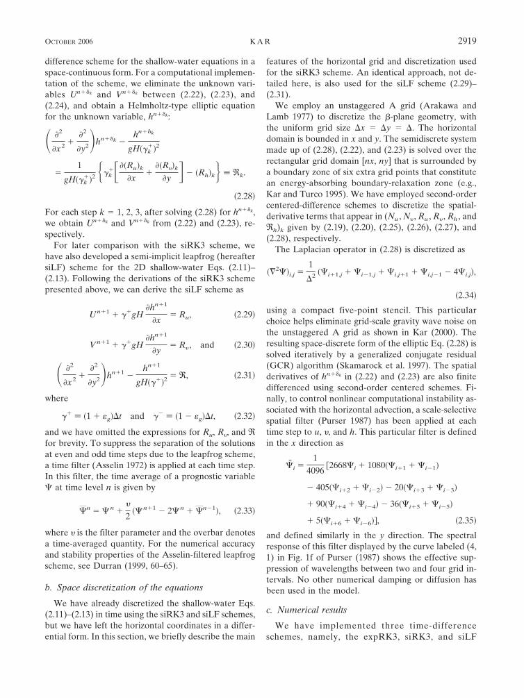
difference scheme for the shallow-water equations in aspace-continuous form. For a computational implemen-tation of the scheme, we eliminate the unknown vari-ables Un�k and Vn�k between (2.22), (2.23), and(2.24), and obtain a Helmholtz-type elliptic equationfor the unknown variable, hn�k:

� �2

�x2 ��2

�y2�hn��k �hn��k

gH��k��2

�1

gH��k��2 ��k

����Ru�k

�x�

��R�k

�y �� �Rh�k� � ℜk.

�2.28�

For each step k � 1, 2, 3, after solving (2.28) for hn�k,we obtain Un�k and Vn�k from (2.22) and (2.23), re-spectively.

For later comparison with the siRK3 scheme, wehave also developed a semi-implicit leapfrog (hereaftersiLF) scheme for the 2D shallow-water Eqs. (2.11)–(2.13). Following the derivations of the siRK3 schemepresented above, we can derive the siLF scheme as

Un�1 � ��gH�hn�1

�x� Ru, �2.29�

Vn�1 � ��gH�hn�1

�y� R , and �2.30�

� �2

�x2 ��2

�y2�hn�1 �hn�1

gH����2 � ℜ, �2.31�

where

�� � �1 � �g��t and �� � �1 � �g��t, �2.32�

and we have omitted the expressions for Ru, R�, and ℜfor brevity. To suppress the separation of the solutionsat even and odd time steps due to the leapfrog scheme,a time filter (Asselin 1972) is applied at each time step.In this filter, the time average of a prognostic variable� at time level n is given by

�n � �n �

2��n�1 � 2�n � �n�1�, �2.33�

where � is the filter parameter and the overbar denotesa time-averaged quantity. For the numerical accuracyand stability properties of the Asselin-filtered leapfrogscheme, see Durran (1999, 60–65).

b. Space discretization of the equations

We have already discretized the shallow-water Eqs.(2.11)–(2.13) in time using the siRK3 and siLF schemes,but we have left the horizontal coordinates in a differ-ential form. In this section, we briefly describe the main

features of the horizontal grid and discretization usedfor the siRK3 scheme. An identical approach, not de-tailed here, is also used for the siLF scheme (2.29)–(2.31).

We employ an unstaggered A grid (Arakawa andLamb 1977) to discretize the �-plane geometry, withthe uniform grid size �x � �y � �. The horizontaldomain is bounded in x and y. The semidiscrete systemmade up of (2.28), (2.22), and (2.23) is solved over therectangular grid domain [nx, ny] that is surrounded bya boundary zone of six extra grid points that constitutean energy-absorbing boundary-relaxation zone (e.g.,Kar and Turco 1995). We have employed second-ordercentered-difference schemes to discretize the spatial-derivative terms that appear in (Nu , N� , Ru , R� , Rh , andℜh)k given by (2.19), (2.20), (2.25), (2.26), (2.27), and(2.28), respectively.

The Laplacian operator in (2.28) is discretized as

� 2��i,j �1

�2 ��i�1,j � �i�1,j � �i,j�1 � �i,j�1 � 4�i,j�,

�2.34�

using a compact five-point stencil. This particularchoice helps eliminate grid-scale gravity wave noise onthe unstaggered A grid as shown in Kar (2000). Theresulting space-discrete form of the elliptic Eq. (2.28) issolved iteratively by a generalized conjugate residual(GCR) algorithm (Skamarock et al. 1997). The spatialderivatives of hn�k in (2.22) and (2.23) are also finitedifferenced using second-order centered schemes. Fi-nally, to control nonlinear computational instability as-sociated with the horizontal advection, a scale-selectivespatial filter (Purser 1987) has been applied at eachtime step to u, �, and h. This particular filter is definedin the x direction as

�̃i �1

40962668�i � 1080��i�1 � �i�1�

� 405��i�2 � �i�2� � 20��i�3 � �i�3�

� 90��i�4 � �i�4� � 36��i�5 � �i�5�

� 5��i�6 � �i�6��, �2.35�

and defined similarly in the y direction. The spectralresponse of this filter displayed by the curve labeled (4,1) in Fig. 1f of Purser (1987) shows the effective sup-pression of wavelengths between two and four grid in-tervals. No other numerical damping or diffusion hasbeen used in the model.

c. Numerical results

We have implemented three time-differenceschemes, namely, the expRK3, siRK3, and siLF

OCTOBER 2006 K A R 2919

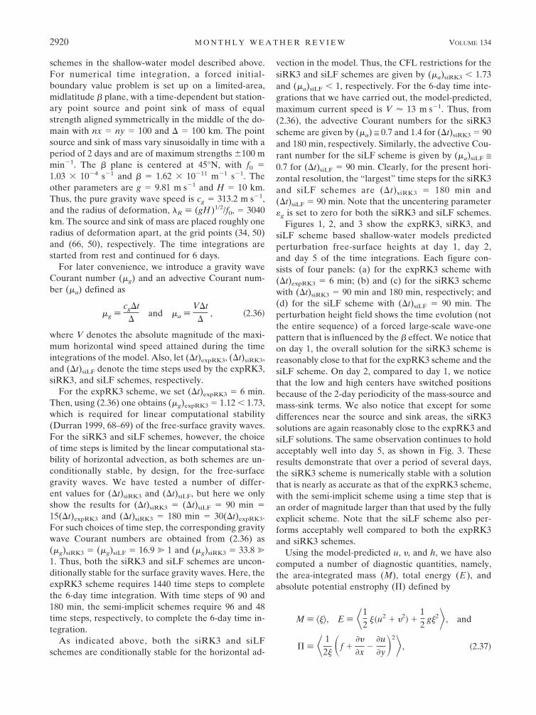
schemes in the shallow-water model described above.For numerical time integration, a forced initial-boundary value problem is set up on a limited-area,midlatitude � plane, with a time-dependent but station-ary point source and point sink of mass of equalstrength aligned symmetrically in the middle of the do-main with nx � ny � 100 and � � 100 km. The pointsource and sink of mass vary sinusoidally in time with aperiod of 2 days and are of maximum strengths �100 mmin�1. The � plane is centered at 45°N, with f0 �1.03 � 10�4 s�1 and � � 1.62 � 10�11 m�1 s�1. Theother parameters are g � 9.81 m s�1 and H � 10 km.Thus, the pure gravity wave speed is cg � 313.2 m s�1,and the radius of deformation, �R � (gH)1/2/f0, � 3040km. The source and sink of mass are placed roughly oneradius of deformation apart, at the grid points (34, 50)and (66, 50), respectively. The time integrations arestarted from rest and continued for 6 days.

For later convenience, we introduce a gravity waveCourant number (�g) and an advective Courant num-ber (�a) defined as

�g �cg�t

�and �a �

V�t

�, �2.36�

where V denotes the absolute magnitude of the maxi-mum horizontal wind speed attained during the timeintegrations of the model. Also, let (�t)expRK3, (�t)siRK3,and (�t)siLF denote the time steps used by the expRK3,siRK3, and siLF schemes, respectively.

For the expRK3 scheme, we set (�t)expRK3 � 6 min.Then, using (2.36) one obtains (�g)expRK3 � 1.12 � 1.73,which is required for linear computational stability(Durran 1999, 68–69) of the free-surface gravity waves.For the siRK3 and siLF schemes, however, the choiceof time steps is limited by the linear computational sta-bility of horizontal advection, as both schemes are un-conditionally stable, by design, for the free-surfacegravity waves. We have tested a number of differ-ent values for (�t)siRK3 and (�t)siLF, but here we onlyshow the results for (�t)siRK3 � (�t)siLF � 90 min �15(�t)expRK3 and (�t)siRK3 � 180 min � 30(�t)expRK3.For such choices of time step, the corresponding gravitywave Courant numbers are obtained from (2.36) as(�g)siRK3 � (�g)siLF � 16.9 � 1 and (�g)siRK3 � 33.8 �

1. Thus, both the siRK3 and siLF schemes are uncon-ditionally stable for the surface gravity waves. Here, theexpRK3 scheme requires 1440 time steps to completethe 6-day time integration. With time steps of 90 and180 min, the semi-implicit schemes require 96 and 48time steps, respectively, to complete the 6-day time in-tegration.

As indicated above, both the siRK3 and siLFschemes are conditionally stable for the horizontal ad-

vection in the model. Thus, the CFL restrictions for thesiRK3 and siLF schemes are given by (�a)siRK3 � 1.73and (�a)siLF � 1, respectively. For the 6-day time inte-grations that we have carried out, the model-predicted,maximum current speed is V � 13 m s�1. Thus, from(2.36), the advective Courant numbers for the siRK3scheme are given by (�a) ≅ 0.7 and 1.4 for (�t)siRK3 � 90and 180 min, respectively. Similarly, the advective Cou-rant number for the siLF scheme is given by (�a)siLF ≅0.7 for (�t)siLF � 90 min. Clearly, for the present hori-zontal resolution, the “largest” time steps for the siRK3and siLF schemes are (�t)siRK3 � 180 min and(�t)siLF � 90 min. Note that the uncentering parameter�g is set to zero for both the siRK3 and siLF schemes.

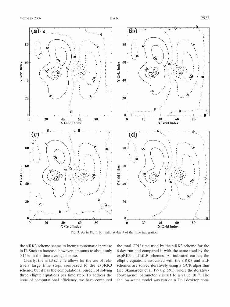
Figures 1, 2, and 3 show the expRK3, siRK3, andsiLF scheme based shallow-water models predictedperturbation free-surface heights at day 1, day 2,and day 5 of the time integrations. Each figure con-sists of four panels: (a) for the expRK3 scheme with(�t)expRK3 � 6 min; (b) and (c) for the siRK3 schemewith (�t)siRK3 � 90 min and 180 min, respectively; and(d) for the siLF scheme with (�t)siLF � 90 min. Theperturbation height field shows the time evolution (notthe entire sequence) of a forced large-scale wave-onepattern that is influenced by the � effect. We notice thaton day 1, the overall solution for the siRK3 scheme isreasonably close to that for the expRK3 scheme and thesiLF scheme. On day 2, compared to day 1, we noticethat the low and high centers have switched positionsbecause of the 2-day periodicity of the mass-source andmass-sink terms. We also notice that except for somedifferences near the source and sink areas, the siRK3solutions are again reasonably close to the expRK3 andsiLF solutions. The same observation continues to holdacceptably well into day 5, as shown in Fig. 3. Theseresults demonstrate that over a period of several days,the siRK3 scheme is numerically stable with a solutionthat is nearly as accurate as that of the expRK3 scheme,with the semi-implicit scheme using a time step that isan order of magnitude larger than that used by the fullyexplicit scheme. Note that the siLF scheme also per-forms acceptably well compared to both the expRK3and siRK3 schemes.

Using the model-predicted u, �, and h, we have alsocomputed a number of diagnostic quantities, namely,the area-integrated mass (M), total energy (E), andabsolute potential enstrophy (�) defined by

M � ���, E � �12

��u2 � 2� �12

g�2�, and

� � � 12� �f �

�

�x�

�u

�y�2�, �2.37�

2920 M O N T H L Y W E A T H E R R E V I E W VOLUME 134

where

��� � � dx dy. �2.38�

Note that by design of the spatial differencing, the area-integrated total mass is conserved in the time-continuous case. For the shallow-water equations in a

continuous form (2.11)–(2.13), it is readily verified thatM, E, and � are conserved in time, provided there areno friction and mass source and sink terms. Eventhough the current test involves a time-dependentsource and sink of mass, it is of interest to look into thetime series of M, E, and � computed from the modelsolutions.

FIG. 1. Solution at day 1 of the 2D shallow-water model (a) using the explicit RK3 scheme with a time step of 6 min, (b) using thesemi-implicit RK3 scheme with a time step of 90 min, (c) using the semi-implicit RK3 scheme with a time step of 180 min, and (d) usingthe semi-implicit leapfrog scheme with a time step of 90 min. Contours of perturbation height (m) are plotted at an interval of 5 m.

OCTOBER 2006 K A R 2921

Figure 4 shows the time series of the model-computed M, E, and � for the expRK3, siRK3, andsiLF schemes. The plotted variables are normalized bytheir respective initial values. The time variations ofboth M and E, irrespective of the schemes, are boundedand relatively small with a quasi-periodicity of 2 days.The siRK3 and siLF solutions closely follow theexpRK3 solution, particularly in terms of phase. In

terms of amplitude, the siRK3 and siLF schemes regis-ter slightly lower absolute magnitudes compared to theexpRK3 scheme. This particular aspect of the siRK3solution is slightly enhanced when the time step is in-creased. Figure 4c shows that the model-computed ab-solute potential enstrophy � also remains bounded andshows very similar phase variations in time for allschemes. Compared with the expRK3 and siLF schemes,

FIG. 2. As in Fig. 1 but valid at day 2 of the time integration.

2922 M O N T H L Y W E A T H E R R E V I E W VOLUME 134

the siRK3 scheme seems to incur a systematic increasein �. Such an increase, however, amounts to about only0.15% in the time-averaged sense.

Clearly, the sirk3 scheme allows for the use of rela-tively large time steps compared to the expRK3scheme, but it has the computational burden of solvingthree elliptic equations per time step. To address theissue of computational efficiency, we have computed

the total CPU time used by the siRK3 scheme for the6-day run and compared it with the same used by theexpRK3 and siLF schemes. As indicated earlier, theelliptic equations associated with the siRK3 and siLFschemes are solved iteratively using a GCR algorithm(see Skamarock et al. 1997, p. 591), where the iterative-convergence parameter � is set to a value 10�6. Theshallow-water model was run on a Dell desktop com-

FIG. 3. As in Fig. 1 but valid at day 5 of the time integration.

OCTOBER 2006 K A R 2923

puter (Intel Pentium 4, 2.80 GHz) using Red Hat Linuxversion 3 as the operating system. The total CPU timeused by the expRK3 scheme, for a 6-day run of theshallow-water model is 28.42 s. The corresponding CPUtimes used by the siRK3 scheme are 13.94 and 10.29 sfor (�t)siRK3 � 90 and 180 min, respectively. The totalCPU time used by the siLF scheme is 7.87 s for(�t)siLF � 90 min. Thus, the siRK3 scheme with a timestep of 180 min costs nearly 30% more compared to thesiLF scheme with a time step of 90 min. Note that theGCR solver used here does not include a precondi-tioner that could accelerate its convergence and

thereby potentially improve upon the current efficiencyof the siRK3 scheme compared to the siLF scheme.

3. Summary

In the framework of a two-dimensional shallow-water model in flux convergence form, a semi-implicitRunge–Kutta time-difference scheme has been devel-oped. The proposed scheme essentially extends an es-tablished explicit third-order Runge–Kutta (expRK3)time-difference scheme into a semi-implicit Runge–Kutta (siRK3) scheme that employs (a) a second-ordertrapezoidal scheme for the gravity wave terms, at eachof the three iterative steps of the third-order Runge–Kutta scheme, but (b) continues to employ the explicitthird-order Runge–Kutta scheme for the nonlinearterms including horizontal fluxes of mass and momen-tum. A linear stability analysis of the proposed schemeis presented in the appendix. The siRK3 scheme re-quires a two-dimensional Helmholtz-type elliptic equa-tion to be solved at each iterative step of the scheme. Aconjugate-residual solver without a preconditioner hasbeen used in the model to solve the aforementionedelliptic equation.

The effectiveness of the siRK3 scheme, compared tothe expRK3 and the semi-implicit (time filtered) leap-frog (hereafter siLF) schemes in terms of numericalstability, accuracy, and efficiency, is establishedthrough an idealized numerical time integration of theshallow-water model. The numerical results show thateven though the siRK3 scheme treats the gravity waveswith second-order accuracy in time, compared to thethird-order accuracy of the expRK3 scheme, the siRK3provides a stable, reasonably accurate, and numericallyefficient solution with relatively large time steps. How-ever, the siRK3 scheme costs about 30% more in termsof CPU time compared to the siLF scheme. The addi-tional computational burden is perhaps bearable inview of the third-order accuracy in time obtained forhorizontal advection using the siRK3 scheme, com-pared to less than second-order accuracy in time for thesame process using the Asselin-filtered siLF scheme.

The proposed siRK3 scheme was implemented in theshallow-water equations in a flux convergence form.This ensures conservation of total mass; however, thesame scheme can also be easily applied to the advectiveform of the shallow-water equations.

The proposed siRK3 scheme can be implemented inthree-dimensional hydrostatic and nonhydrostatic mod-els, once the semi-implicit linearization of the appro-priate governing equations is established. The proposedscheme can also be adapted to semi-Lagrangian dynam-ics, if we employ a backward-trajectory-based semi-

FIG. 4. Time evolution of the area-integrated (a) mass, (b) totalenergy, and (c) absolute potential enstrophy. Each quantity isnormalized by its initial value. The solid curve is for the explicitRK3 scheme with �t � 6 min. The dotted and dashed curves arefor the semi-implicit RK3 scheme with �t � 90 and 180 min,respectively. The dotted–dashed curve is for the semi-implicitleapfrog scheme with �t � 90 min.

2924 M O N T H L Y W E A T H E R R E V I E W VOLUME 134

Lagrangian advection scheme to each of the three it-erative steps of the scheme. Some of these issues will beaddressed in the future.

Acknowledgments. The author is thankful to Drs. R.James Purser and Joseph Sela for helpful comments onthe original draft, and Mary L. Hart for editorial im-provements. The author greatly appreciates the review-ers’ comments in significantly improving the paper.

APPENDIX

Linear Stability Analysis of the siRK3 Scheme

To perform a von Neumann stability analysis of thesiRK3 scheme, let us substitute

L��� � i�� and N��� � i�� �A.1�

into (2.10). Here, � and � denote the relatively high andlow frequencies of �, and i � ��1. Then, (2.10) canbe expanded into the following component steps:

�1 � i�1�g���t��* � 1 � i�1��g

���t � ��t���n,

�A.2�

�1 � i�2�g���t��** � �1 � i�2�g

���t��n

� �i�2��t��*, and �A.3�

�1 � i�g���t��n�1 � �1 � i�g

���t��n � �i��t��**,

�A.4�

where

�g� �

12

�1 � �g� and �g� �

12

�1 � �g�. �A.5�

Eliminating the variables �* and �** from (A.2)–(A.4), we can derive the (complex) amplification factor� defined by

� � �n�1��n, �A.6�

in terms of the constants ��g and ��

g , and the variables��t and ��t. Note that for stability of the siRK3scheme, one must satisfy the condition |� | � 1.

When � � 0 and � � 0, (2.10) reduces to the expRK3scheme with the amplification factor

� � �1 �12

���t�2�� i���t �16

���t�3�. �A.7�

This leads to

|� |2 � 1 �1

12���t�4 �

136

���t�6, �A.8�

so that for the stability of the expRK3 scheme, |� | � 1or |��t | � �3 � 1.73 must be satisfied.

However, when � � 0 and � � 0, the algebraic ex-pression (not shown) for |� | does not readily yield anexplicit inequality in terms of ��t and ��t. To addressthis issue numerically, we have plotted the contours of|� | as a function of ��t and ��t in Fig. A1. Here wehave assumed �g � 0, for simplicity. The dashed con-tours of |� | valued greater than unity display the un-stable region. The region of stability is recognized bythe solid contours of |� | valued less than unity. Clearly,the stable region is limited by ��t � 1.73, for all valuesof ��t. Thus, the siRK3 scheme is conditionally stablewith the stability restriction, ��t � 1.73, which is essen-tially dictated by the explicit RK3 part of the scheme, asexpected.

REFERENCES

Arakawa, A., and V. R. Lamb, 1977: Computational design of thebasic dynamical processes of the UCLA general circulationmodel. Methods in Computational Physics, J. Chang, Ed.,Vol. 17, Academic Press, 173–265.

Ascher, U. M., S. J. Ruuth, and R. J. Spiteri, 1997: Implicit–explicit Runge–Kutta methods for time-dependent partialdifferential equations. Appl. Numer. Math., 25, 151–167.

FIG. A1. The modulus of the amplification factor � as a functionof ��t and ��t for the semi-implicit RK3 scheme applied to theoscillation equation: dt� � i��, where �(� � � �) is the angularfrequency. The contour interval is 0.1. The solid and dashed con-tours, respectively, are used to display the stable (|� | � 1) andunstable (|� | � 1) regions of the (��t, ��t) parameter space.When ��t � 0, |� | � 1 for all values of ��t, along the ��t axis.

OCTOBER 2006 K A R 2925

Asselin, R., 1972: Frequency filter for time integrations. Mon.Wea. Rev., 100, 487–490.

Butcher, J. C., 1964: Implicit Runge–Kutta processes. Math. Com-put., 18, 50–64.

——, 1987: The Numerical Analysis of Ordinary DifferentialEquations: Runge–Kutta and General Linear Methods. JohnWiley and Sons, 512 pp.

Durran, D. R., 1999: Numerical Methods for Wave Equations inGeophysical Fluid Dynamics. Springer-Verlag, 465 pp.

Gear, C. W., 1971: Numerical Initial Value Problems in OrdinaryDifferential Equations. Prentice-Hall, 253 pp.

Kar, S. K., 2000: Stable centered-difference schemes, based on anunstaggered A grid, that eliminate two-grid interval noise.Mon. Wea. Rev., 128, 3643–3653.

——, and R. P. Turco, 1995: Formulation of a lateral sponge layerfor limited-area shallow-water models and an extension forthe vertically stratified case. Mon. Wea. Rev., 123, 1542–1559.

Kwizak, M., and A. J. Robert, 1971: A semi-implicit scheme for

grid point atmospheric models of the primitive equations.Mon. Wea. Rev., 99, 32–36.

Purser, R. J., 1987: The filtering of meteorological fields. J. Cli-mate Appl. Meteor., 26, 1764–1769.

Robert, A. J., 1969: The integration of a spectral model of theatmosphere by the implicit method. Proc. WMO–IUGGSymp. on Numerical Weather Prediction, Vol. VII, Tokyo,Japan, Japan Meteorological Agency, 19–24.

Skamarock, W. C., P. K. Smolarkiewicz, and J. B. Klemp, 1997:Preconditioned conjugate-residual solvers for Helmholtzequations in nonhydrostatic models. Mon. Wea. Rev., 125,587–599.

——, J. B. Klemp, and J. Dudhia, 2001: Prototypes for the WRF(Weather Research and Forecasting) model. Extended Ab-stracts, Ninth Conf. on Mesoscale Processes, Fort Lauderdale,FL, Amer. Meteor. Soc., J1.5.

Wicker, L. J., and W. C. Skamarock, 2002: Time-splitting methodsfor elastic models using forward time schemes. Mon. Wea.Rev., 130, 2088–2097.

2926 M O N T H L Y W E A T H E R R E V I E W VOLUME 134