A semi-empirical ship operational performance prediction modelfor voyage optimization towards energy efficient shipping

Ruihua Lu n, Osman Turan, Evangelos Boulougouris, Charlotte Banks, Atilla IncecikDepartment of Naval Architecture and Marine Engineering, University of Strathclyde, 100 Montrose Street, Glasgow G4 0LZ, UK

a r t i c l e i n f o

Article history:Received 3 February 2015Accepted 22 July 2015Available online 8 September 2015

Keywords:Energy efficient shippingVoyage optimizationShip operational performanceFuel savingCo2 emission reduction

a b s t r a c t

Voyage optimization is a practice to select the optimum route for the ship operators to increase energyefficiency and reduce Green House Gas emission in the shipping industry. An accurate prediction of shipoperational performance is the prerequisite to achieve these targets. In this paper, a modified Kwon'smethod was developed to predict the added resistance caused by wave and wind for a specific ship type,and an easy-to-use semi-empirical ship operational performance prediction model is proposed. It canaccurately predict the ship's operational performance for a specific commercial ship under differentdrafts, at varying speeds and in varying encounter angles, and then enables the user to investigate therelation between fuel consumption and the various sea states and directions that the ship mayencounter during her voyage. Based on the results from the operational performance prediction modeland real time climatological information, different options for the ship's navigation course can beevaluated according to a number of objectives, including: maximizing safety and minimizing fuelconsumption and voyage time. By incorporating this into a decision support tool, the ship's crew are ableto make an informed decision about what is the best course to navigate.

In this study the Energy Efficiency of Operation (EEO) is defined as an indicator to illustrate the ratioof main engine fuel consumption per unit of transport work. Two case studies are carried out to performthe prediction of ship operational performance for Suezmax and Aframax Oil Tankers, and the resultsindicate that the semi-empirical ship operational performance prediction model provides extremelyquick calculation with very reasonable accuracy, particularly considering the uncertainties related to theparameters of interest for the case study data. Within the case studies, the additional fuel consumptioncaused by the combined hull and propeller fouling and engine degradation is included in the model as atime-dependent correction factor. The factor may assist the ship owner/operator to determine the hullcoating selection, and/or the dry-docking and main engine maintenance strategy.& 2015 The Authors. Published by Elsevier Ltd. This is an open access article under the CC BY license

(http://creativecommons.org/licenses/by/4.0/).

1. Introduction

Energy efficient shipping is a prerequisite for the reduction ofthe Green House Gas (GHG) emissions to the levels anticipatedwithin the next decades. The continuous growth of the worldpopulation and the increase number of developing countries led tothe increasing dependence of the world economy on the interna-tional trade. For 2007, it was estimated that shipping emits 1046million tonnes of CO2 from exhaust emissions, accounting for 3.3%of the global CO2 emission during that year. CO2 emission fromInternational shipping alone were estimated to account 2.7% of theglobal CO2 emission in 2007, and the carbon dioxide emissionsfrom international shipping was projected to triple by the year

2050 (IMO, 2009). These findings alerted the International Mar-itime Organization (IMO) and led to the introduction of the firstmaritime energy efficiency regulations that entered into force onthe 1st of January 2013 (IMO, 2011). The aim of the regulations is toreduce carbon emissions by decreasing the amount of fuel con-sumed. This can be achieved by optimizing the ship’s design,deploying new energy efficient technologies, or by improving theship’s operation. The regulations require both new and existingship above 400 GT to have a ship specific Ship Energy EfficiencyManagement Plan, SEEMP (IMO, 2012).

An additional drive towards a more energy efficient shipping isthe requirement to remain competitive within a fierce market.Although marine engines used for commercial shipping use thecheapest type of ‘bunker fuel’, the cost of IFO 180 has risen sharplywith other petroleum products, increasing from $170/t in 2002,and from $230/t in 2005, to nearly $700/t in July 2014 (BunkerIndex, 2014). With such high fuel prices, the bunker costs couldaccount for 50–60% of a ship's total operating costs (Wang and Teo,

Contents lists available at ScienceDirect

journal homepage: www.elsevier.com/locate/oceaneng

Ocean Engineering

http://dx.doi.org/10.1016/j.oceaneng.2015.07.0420029-8018/& 2015 The Authors. Published by Elsevier Ltd. This is an open access article under the CC BY license (http://creativecommons.org/licenses/by/4.0/).

n Corresponding author at: Department of Naval Architecture, Ocean and MarineEngineering, University of Strathclyde, 100 Montrose Street, Glasgow G4 0LZ, UK.Tel.: +44 1415484165.

E-mail address: r.lu@strath.ac.uk (R. Lu).

Ocean Engineering 110 (2015) 18–28

2013). The rising fuel price has supported the increasing need forenergy efficiency to survive in highly competitive and capacityoversupplied shipping market.

It is important to realize that an optimum route cannot only beevaluated in terms of fuel consumption. Normally, the voyageoptimization has multiple, often conflicting, objectives, such as:minimizing costs regardless of arrival time; punctual time ofarrival; safety; and passenger comfort. In most cases, improvingone objective may reduce efficiency of another. Each attributetherefore requires a weighting of importance. For example, someshipping companies' business models prioritise on-time arrivaland shorter transit times over reduced fuel consumption. For othercompanies, providing a ‘green service’ has a higher priority.

Most existing techniques and software solutions for voyage opti-mization extract the ship's operational performance from a databasebuild on results from similar ships (in terms of type and size).However, the performance of each specific ship in various voyageconditions (speed, fouling and propulsion system degradation, anddraft) may be quite different, especially under severe weather condi-tions. This highlights the need for real-time, flexible ship-specificmodeling in order to provide increased accuracy of ship operationalperformance prediction for voyage optimization. Another commondisadvantage of many existing voyage optimization software solutionsis that they only present to the ship's master the recommended route.The users of the software cannot test their intended route andcompare its performance to the software recommended route. As aresult, captains may develop mistrust to the recommended route andproceed according to their own judgement.

Voyage optimization software can be evaluated according to:

� Technical status – the accuracy and practicability of shipoperational performance prediction.

� User acceptance – the user friendliness.� Economic performance – the evaluation of fuel saving based on

voyage optimization.

These three evaluation principles are also the objectives of theresearch presented. This paper focuses on the development of anaccurate and practical ship operational performance predictionmodel that can be used to select the optimum routes for minimumfuel consumption, taking into consideration average ship speed,encountering sea states and voyage time.

The ship operational performance model presented in this paperis developed by the modifying Kwon's method (Kwon, 2008) usinga case study of ship's operational data (i.e. ship's noon reports) andsea trial data. The Kwon's method (Kwon, 2008) is an empiricalmethod for the prediction of added resistance due to sea state andwave directions. The case study of ship's operational data is taken asthe reference for the modified Kwon's method. This modified modelcan predict the ship's operational performance for a givenwave andweather condition at different speeds, drafts and wave encounterangle in a semi-empirical way.

A decision support tool has been developed to select the optimumcourse according to the users' preference. The users can influence theselection of the optimized route by providing different weightings tothe optimization objectives (see optimum route a–e listed in Fig. 10).

Besides the development of the ship operational performanceprediction and the optimum routes selection, a time-dependentfuel consumption increase rate after ship dry-docking has beenidentified, which may be helpful in monitoring ship fouling andengine degradation condition. The identified fuel consumptionrate of increase will further assist shipping companies withplanning dry-docking and engine maintenance scheduling.

2. State of the art

2.1. Semi-empirical approaches for predicting the added resistance

The prediction of ship total resistance in waves (RT) cantypically be performed in two steps (ITTC, 2011):

a) Prediction of still water resistance, RSW, at speeds of interest.b) Prediction of added resistance in waves, RAW, at the same

speeds.

The prediction of ship total resistance in waves is obtained bysumming the above mentioned predicted values:

RT ¼ RSW þRAW ð1Þseveral methods are available to determine the still water resis-tance of ships. In the presented analysis the Holtrop and Mennenmethod (Holtrop and Mennen, 1982) has been used.

The increase in resistance caused by waves, greater than the stillwater condition, can also be calculated using several methods, includ-ing Strip Method, Radiated Energy Method, Rankine Panel Method,Cartesian Grid Method, CFD Method, Experiment Method, EmpiricalMethod, and Semi-empirical Method. In the following section,some of the semi-empirical methods for added resistance predictionare reviewed.

2.1.1. The approximated – Salvesen methodThe Salvesen method (Salvesen, 1978) provides a basic formula

for the added resistance calculation.

RAW ¼ � i2k cos β

Xj ¼ 3;5

ξj FIn

j þ F̂Dj

n oþR7 ð2Þ

where F̂In

j , is the complex conjugate of the Froude-Krilov part of theexciting force and moment, and F̂

Dj is very similar to the diffraction

part of the existing force FDj , k is the wave number, βis wave headingdirection, and ξj is the motion calculated by the strip theory. R7 isgiven by

R7 ¼ �12ξ2I k

ω2

ωecos β

ZLe�2kdsðb33þb22 sin

2βÞdx ð3Þ

Where, ξI is the incident wave amplitude, b33 and b22 are the sectionalheave and sway damping coefficient, d is the sectional draft and s isthe sectional-area coefficient. Details of formula 2 and 3 are presentedin Salvesen (1978).

The Salvesen method is able to provide accurate results for thelonger waves regions (L/λo1.5). Therefore, to extend its use forshort wave length regions a correction is added to the originalSalvesen method to produce the approximated – Salvesen method(Matulja et al., 2011). The correction contains an approximatedformula proposed by Faltinsen et al. (1980):

RAW ¼ 12ρg 1þ2ωU

g

� � ZL1

sin 2νn1dl ð4Þ

where, L1 is non shadow zone of the water plane area, U is shipspeed, ω is Encounter frequency, n1 is X component of the inwardnormal n to the water line, and ν is the angle between the tangentto the water line and the x axis.

The final step of the approximated – Salvesen method is:

R¼ a for L=λr1 ð5Þ

R¼ aþb for 1oL=λr2 ð6Þ

R¼ b for L=λ42 ð7Þ

R. Lu et al. / Ocean Engineering 110 (2015) 18–28 19

where,

a¼ � i2k cos β

Xj ¼ 3;5

ξi FIn

j þ F̂Dj

n oð8Þ

b¼ 12ρg 1þ2ωU

g

� � ZL1

sin 2vn1dl ð9Þ

However, formula 8 is only valid in wave heading directionβ� 180o if the speed U is high, and for β� 90o if the speed U islow. The full range of heading directions experienced by a ship inpractice are therefore not accounted for with this method. This is adisadvantage for accurate ship performance prediction. Further-more, the definition of the term ‘short waves region’ is looselydefined as it is related to the ship length, further increasing theuncertainty in the added resistance prediction.

In an overall view of the approximated – Salvesen method, theFaltinsen's approximated formula was used to evaluate wavereflection added resistance and then the Salvesen's results werecombined with the wave reflection added resistance in a semi-empirical way.

2.1.2. Fuji-Takahashi methodThe Fuji-Takahashi method (Fuji and Takahashi, 1975) is a semi-

empirical method considering the drift force acting on an uprightbarrel and then correcting these forces with a coefficient for shipshape & speed. The drift force is calculated using the followingequation:

D¼ 12ρgξ2a

Z B=2

�B=2sin 2βdy ð10Þ

where, ξa is the amplitude of the incident waves, ρ is sea waterdensity, g is gravitational acceleration, β is an inclination angle forx-axis on the hull, B is ship breadth.

The added resistance generated by the reflected wave RAW iscalculated by:

RAW ¼ α1ð1þα2Þ12ρgξ2a

Z B=2

�B=2sin 2βdy ð11Þ

α1 ¼π2I1ðkdÞ2

π2I1ðkdÞ2þK1ðkdÞ2ð12Þ

α2 ¼ 5ffiffiffiffiffiFn

pð13Þ

where, α1, α2, d, and k denote coefficients for the draft effect, shipspeed effect, draft, wave number, and Fn is Froude number.

The semi-empirical formula of Fuji-Takahashi is a widely usedto predict ship added resistance, but the added resistance due toreflected waves acting on the bulbous-bow is not included. Thismay lead to significant error in predicting the added resistance asbow flare above the water surface may change the reflectedwave properties, along with the presence of the bulbous bowunder water.

2.1.3. Kuroda-Tsujimoto-Fujiwara-Ohmatsu-Takagi methodBased on the investigation of Fuji and Takahashi's (1975) semi-

empirical method, Kuroda et al. (2008) proposed an improvedexpression for the added resistance due to wave reflection (RAW ).The formula is as follows:

RAW ¼ 12ρgξ2aαdð1þαUÞBBf ðχÞ ð14Þ

where, αd is effect of draft and frequency, 1þαU is effect ofadvance speed, Bf is bluntness coefficient, and χ indicates shipheading direction.

Kuroda et al. modified the terms for added resistance due towave reflection by taking into account the effect of draft, waveencounter frequency and speed of advance. The oblique waveswere also applied on the method. Kuroda-Tsujimoto-Fujiwara-Ohmatsu-Takagi method requires tank testing in short waves andtherefore the effect of hull form above water line is captured in theadded resistance calculation. However, the added resistance due toreflected waves acting on bulbous-bow is still not included.

2.1.4. A simplified method to calculate added resistance based onGerritsma and Beukelman's method

Gerritsma and Beukelman’s method (Gerritsma and Beukelman,1972) considers radiated energy to calculate added resistance.

The added resistance is calculated with the following expres-sion:

RAW ¼ �k cos β2

2ωe

Z L

0b0 jVZb

j 2℘xb ð15Þ

where, k is wave number, β is heading angle, ωe is frequency ofencounter, L is ship's water line length, jVZb

j is the amplitude ofthe velocity of water relative to the strip, b0is the sectionaldamping coefficient for speed, xb is x coordinate on the ship.

The Gerritsma and Beukelman's method (Gerritsma andBeukelman, 1972) is one of the most widely used added resistancemodeling methods that utilize Strip Theory, and it provides anaccurate added resistance prediction across the different shiptypes. However, for added resistance calculation, calculating shipmotions by strip theory is complex and might be unnecessaryin some applications. To address this issue a further simplifiedmethod developed by Alexandersson (2009) was proposed for theadded resistance calculation. The simplified method uses theGerritsma and Beukelman's method, applying to a large series ofcase studies to determine the added resistance, then using linearregression, a series of simplified formulas to determine the addedresistance are derived. This simplified method is therefore a semi-empirical method as it uses the results from the Gerritsma andBeukelman’s analytical method (Gerritsma and Beukelman, 1972)and combines it with regression techniques.

Although the semi-empirical method simplifies the more com-plicated strip theory calculations whilst still providing relativelystable predictions for added resistance, the limitations of themethod still exist, such as the prediction accuracy decreases inbow/beam/following waves and high frequency waves; trim of theship is not included.

2.1.5. Summary of semi-empirical methods to predict addedresistance

In an overview of the existing semi-empirical methods foradded resistance prediction, they either combine empirical meth-ods with analytical results, or update existing empirical methodwith analytical method, in a semi-empirical way. The commondisadvantage for these methods is that they are not able to predictthe added resistance accurately with different encounter angle.The short or long wave length is also a critical parameter forselecting the right formulas. The semi-empirical methods, whichinvolve tank tests, may sharply increase the modeling cost as itmay take much longer time for added resistance estimation.

2.2. Voyage optimization in routing service

Extensive surveys of research on ship routing and schedulinghave been carried out about every 10 years (Ronen, 1983, 1993;Christiansen et al., 2004, 2013). Fagerholt et al. (2010) proposedmathematical models to optimize speed on a ship route. However,the fuel consumption was approximated by a cubic function,

R. Lu et al. / Ocean Engineering 110 (2015) 18–2820

which is not accurate enough for voyage optimization. Padhy et al.(2008) predicted the speed loss due to weather condition usingsea-keeping computing tools. The pre-computed Response Ampli-tude Operator (RAO) was employed in Dijkstra's algorithm toobtain optimum route in a given sea-state. Hinnenthal andGlauss (2010) utilized strip-theory and wave spectra to generateRAO, and predicted the added resistance through a statisticalevaluation method for voyage optimization. Avgouleas (2008)estimated mean added resistance in waves with the aid of SWAN1,which is an advanced frequency domain CFD code using RankinePanel Methods. Then the Iterative Dynamic Programming algo-rithm was employed to achieve voyage optimization. The ship'sresponse based routing and high fidelity computational hydro-dynamic performance based routing require huge amount ofcomputations, long simulation time and the up-to-date shipconditions are not involved. It seems to be immature for accurateand efficient voyage optimization. Larsson and Simonsen (2014),and Shao (2013) adopted Kwon's method (Kwon, 2008) to predictadded resistance for weather routing. However, Kwon's method isa generic approach for large number of commercial ship types.Therefore, regarding the limited accuracy of added resistance andship operational performance modeling for specific commercialship, the accuracy of voyage optimization can be further increased.

The ship routing service can generally be categorized intoashore based routing services, on-board based routing servicesand the combination of ashore and on-board routing services.Table 1 provides an overview of available ship routing service.

3. Data description

Ships have to collect operational data on a daily basis, known asship logs and ship reports (often referred to as noon reports asthey are typically recorded every 24 h at noon). The type of datafields that are included in the ship reports cover: date/time of thereport, ship position, and estimated time of arrival, arrival/depar-ture port, observed distance, achieved speed, mean draft, BeaufortNumber, wind direction, and total main engine fuel consumption

per day. There is no standard for the recording of operationalparameters within the ship reports and therefore the contenttends to differ between companies compared to the parametersmentioned above. These parameters contain a vast amount ofuncertainty. This uncertainty originates from the methods used toobtain their measurement, the type of measurement, human errorand the assumptions made during analysis. Some of the uncer-tainties related to the parameters of interest for the case studydata are discussed here:

� Achieved speed: the achieved speed is calculated by dividingthe observed distance recorded by the report duration. Thespeed is therefore given as an average value for the wholereport duration. It does not take into account the speed profilewhich, due to the approximately cubic relationship betweenship speed and power, could have a significant influence overthe fuel consumed during the reporting period. The achievedspeed is also the speed over ground and therefore, the effects ofcurrents and tides are not taken into account. To improve theaccuracy of performance prediction, the speed through watershould be obtained.

� Beaufort Number (BN): the Beaufort measurement itself con-tains uncertainty as one number is used to represent a range ofwave heights and sea conditions. More accurate added resis-tance performance prediction methods depend on the waveheight as an input along with the type of sea spectrum(including surface waves and developed seas). Additionaluncertainty is created with the measurement of BeaufortNumber being made via judgement of the sea conditionstypically out of the window on the bridge by the officer onwatch. Not only is this measurement subjective as it is ajudgement, it is also observed from some distance away fromthe sea surface. There is also ambiguity as to whether theBeaufort Number recorded is representative of the conditionsat the observation point, or an average of the conditionsobserved over the report duration.

� Wind direction: recording of the wind direction is typicallyaided by the use of an anemometer. Obstructing super

Table 1Exemplary compilation of routing service or decision support systems (Hinnenthal and Clauss, 2010).

Service provider InstalledLocation

Service/System Weatherforecast

Routeplanning

Routeoptimization

Shipmonitoring

Datarecording

Aerospace and MarineInternational (USA)

ashore Weather 3000, internet service, maps displaying fleetand weather information

X X

Weather Routing Inc. (USA) ashore routing advice and Dolphin navigation programcombined with a web-based interactive site

X X

Finish Meteorological Institute(Finland)

ashore weather and routing advice for the Baltic sea X X

Fleetweather (USA) ashore Meteorological consultancy X X XMetworks Ltd. (UK) ashore meteorological consultancy X XApplied Weather Technology (USA) on-board BonVoyage System X XEuronav (UK) on-board seaPro, software or fully integrated bridge system X X XGermanischer Lloyd, Amarcon B.V.(Germany, Netherlands)

on-board SRAS – Shipboard Routing Assistance System X X X

Transas (UK) on-board ship guard SSAS, software or integrated to bridge system X X X XNorwegian met office, C-Map(Norway, Italy)

on-board C-STAR X X

US Navy (USA) on-board STARS X X X XMeteo Consult (Netherlands) on-board SPOS - Ship Performance Optimization System X X X XOceanweather INC., Ocean SystemsINC. (USA)

on-board VOSS – Vessel Optimization and Safety System X X X X

Weather News International,Oceanwaves (USA, Japan)

ashore &on-board

voyage planning system VPS and ORION, routing andoptimization software

X X X

Swedish Met and HydrologyInstitute (Sweden)

ashore &on-board

Seaware Routing, Seaware Routing Plus and SeawareEnRoute Live

X X X

Deutscher Wetterdienst (Germany) ashore &on-board

MetMaster, MetFerry, routing system, advice on demand X X X

R. Lu et al. / Ocean Engineering 110 (2015) 18–28 21

structure in different wind directions is known to produceinaccuracies in the measurement, along with variations in windstrength at different heights. Uncertainty due to averagedmeasurements also applies in the same way as for BeaufortNumber. Furthermore, the wind direction is assumed to be thesame as the wave direction, which may be true in mostinstances of surface waves, but it could also be very differentfor swell direction. To improve sea and wind condition mea-surements the wave, swell and wind direction and strength orheight, should be recorded.

� Ship heading direction: the angle between the direction of shipbow and the North Pole. The angle is measured clockwise fromnorth, in degrees from 01 to 3591.

� Encounter angle: derived fromwind direction, which is relativeto the ship. It is also known as the weather direction, aspresented in Fig. 1.

� Main engine fuel consumption: fuel flow meters improve theaccuracy of fuel consumption measurements if they are cali-brated and working correctly. However, in most cases the mainengine fuel oil consumption is recorded by tank sounding. Notonly could the measurement contains a vast amount of inaccu-racy, but there is room for error in the tank sounding calcula-tions and the recorded value is susceptible to transcriptionerror and intentional alteration for various reasons.

Despite all of the uncertainties described, the parameters in theship reports provide an insight into the operating conditions of theship in sailing and thus provide a value to performance predictionmodeling.

4. Model description

The method for a new semi-empirical approach proposedwithin this paper that can be used for modeling ship operationalperformance is introduced in this section. A modified Kwon'smethod is developed to enhance the accuracy of added resistanceprediction. This method is based on Kwon (2008) added resistancemodeling method but is updated to take into account ship specificcharacteristics by utilizing the analysis of collected operationaldata. The first step of the semi-empirical method is the estimationof the still water resistance. This is followed by the prediction ofadded resistance due to wind and wave conditions.

4.1. Still water resistance modeling

The well-known Holtrop and Mennen's Method (Holtrop andMennen, 1982) is used to estimate the still water resistance of theship. This method is widely used to calculate the total still waterresistance of a ship with a good accuracy for a wide range of shiptypes, sizes, hull forms and for a range of Froude numbers.

4.2. Added resistance modeling

Kwon (2008) added resistance model is an approximate methodfor predicting speed loss of a displacement type ship due to addedresistance in weather conditions (irregular waves and wind). Theadvantage of this method is that it is easy and practical to use.

The weather effect, presented as speed loss, compares thespeed of the ship in varying actual sea conditions to the ship'sexpected speed in still water conditions. It is expressed in thefollowing way using Kwon's method for modeling added resis-tance (Kwon, 2008):

ΔVV1

100%¼ CßCUCForm ð17Þ

V2 ¼ V1�ΔVV1

100%� �

1100%

V1 ¼ V1�ðCßCUCFormÞ1

100%V1 ð18Þ

where,

V1: Design (nominal) operating ship speed in still waterconditions (no wind, no waves), given in m/s.V2: Actual ship speed in the selected weather (wind andirregular waves) conditions, given in m/s.ΔV¼V1�V2 Absolute speed loss, given in m/s.Cß: Direction reduction coefficient, dependent on the weatherdirection angle (with respect to the ship's bow) and theBeaufort Number (BN), as shown in Table 2.CU : Speed reduction coefficient, dependent on the ship's blockcoefficient CB. The loading condition and the Froude Number(Fn), as shown in Table 3.Cform : Ship form coefficient (Cform), as shown in Table 4.

Fig. 1. Encounter angle.

Table 2Direction reduction coefficient Cb due to weather direction.

Weather direction Encounter angle (deg) Direction reduction coefficient Cb

Head sea (irregular wave) and wind 0–30 2Cb ¼ 2Bow sea (irregular wave) and wind 30–60 2Cb ¼ 1:7�0:03ð BN�4ð Þ2ÞBeam sea (irregular wave) and wind 60-150 2Cb ¼ 0:9�0:06ð BN�6ð Þ2ÞFollowing sea (irregular wave) and wind 150–180 2Cb ¼ 0:4�0:03ð BN�8ð Þ2Þ

Table 3Speed reduction coefficient Cu due to Block coefficient Cb .

Block coefficient Cb Ship loading conditions Speed reduction coefficient Cu

0.55 normal 1.7�1.4Fn�7.4Fn2

0.6 normal 2.2�2.5Fn�9.7Fn2

0.65 normal 2.6�3.7Fn�11.6Fn2

0.7 normal 3.1�5.3Fn�12.4Fn2

0.75 loaded or normal 2.4�10.6Fn�9.5Fn2

0.8 loaded or normal 2.6�13.1Fn�15.1Fn2

0.85 loaded or normal 3.1�18.7Fnþ28.0Fn2

0.75 ballast 2.6�12.5Fn�13.5Fn2

0.8 ballast 3.0�16.3Fn�21.6Fn2

0.85 ballast 3.4�20.9Fnþ31.8Fn2

R. Lu et al. / Ocean Engineering 110 (2015) 18–2822

The Kwon's method (Kwon, 2008) provides a general introduc-tion to the calculation of ship speed loss in different weather andsea conditions based on the ship's hull form, encounter angleand sea state. However, the method is not able to provide avery accurate prediction of added resistance for each specificship. Therefore, the modified Kwon's added resistance modelingmethod developed and presented in this paper includes uniquedirection reduction coefficients, speed reduction coefficients andship form coefficients for specific ship type and size. Thesecoefficients are determined from the analysis of the recorded shipoperational data. The case studies in Section 6 will be used toverify that the modified Kwon's method is a practical way toprovide increased accuracy for the prediction of a specific ship'sfuel consumption at varying speeds, encounter angles, drafts andsea states.

4.3. Ship operational performance modeling

Since the ship still water resistance has been predicted utilizingHoltrop and Mennen's Method (Holtrop and Mennen, 1982), therelation between vessel speed (U), total still water resistance(Rtotal), and the required effective power ðPEÞ can be extracted.

PE ¼ RtotalnU ð19ÞAs the added resistance has been modeled by utilizing themodified Kwon's method, the speed loss under varying drafts,Beaufort Number (BN) and encounter angles has been modeled forspecific commercial ship. The corresponding original still waterspeed (V cosw) can be calculated by combining the actual shipspeed (Vactual) in a seaway and speed loss (V loss) due to addedresistance.

V cosw ¼ VactualþV loss ð20ÞThus, under specific BN and ship heading direction, there is acorresponding original still water speed (V cosw) for an actual shipspeed (Vactual). Based on formula 19, for each still water speed,there is a corresponding required effective power. The relationshipbetween actual ship speed (Vactual) and required effective powerðPEÞ can be extracted.

From effective power the required brake power ðPBÞ of mainengine can then be determined as:

PB ¼PE

ηTð21Þ

where ηT is the total power transmission efficiency (from brakepower of main engine to effective power):

ηT ¼ ηHnηOnηRnηS ð22Þwhere, ηH is the hull efficiency; ηO is the open water efficiency; ηRis the relative rotative efficiency; ηS is the shaft efficiency.

The four efficiencies above can be generally estimated throughempirical formulae. However, from the point of view of accurateoperational performance prediction for specific commercial ship, theutilization of Speed-Power Curve in the sea trial documents can beused to extract total power transmission efficiency. When sea trialdocuments are available, for each specified speed, the total powertransmission efficiency can be calculated using the Holtrop and

Mennen's method (Holtrop and Mennen, 1982) to determine theeffective power and the Speed-Power Curve from sea trial documentsto read the corresponding brake power of main engine. Since the totalpower transmission efficiency has been determined, the relationshipbetween actual ship speed and required engine power under varyingsea states is generated.

For each specific ship, the corresponding main engine perfor-mance documents contain the expected fuel consumption basedon ISO reference conditions, which illustrate the Specific Fuel OilConsumption (SFOC) with corresponding engine load, enginepower and engine speed. The ship main engine Fuel ConsumptionRate (FCR) can be determined as:

FCR¼ PBnSFOC ð23ÞFinally, the ship main engine fuel consumption rate under varyingspeeds, sea states, drafts, and ship heading directions can be predicted.

4.4. Weather and sea state modeling

To use the performance prediction model described as part of avoyage optimization model, a source of weather and sea stateforecasting needs to be identified as an input. A ‘GRIB2’ oceanweather forecast file from the National Oceanic and AtmosphericAdministration (NOAA) (2015) is used for this purpose. The decodingprogram has been written in house to read and output the globalocean weather forecast, as presented in Fig. 2. The informationcontained in the file includes significant wave height, swell, windspeed, and directions.

A flow diagram of the semi-empirical method proposed in thispaper to predict the ship operational performance is shown inFig. 3. The dashed boxes on the left indicate the inputs for thisproposed model, and the modeling steps are shown in the solidboxes. The relationship flow between the inputs and modelingsteps has been illustrated with arrows.

5. Voyage optimization

In this section, the development of grids system and utilizationof the proposed performance prediction model in selecting theoptimum route are illustrated. At this stage, the optimumroute is defined as the one with minimum fuel consumptionregarding given average ship speed, encountering sea states andvoyage time.

5.1. Setting up grids

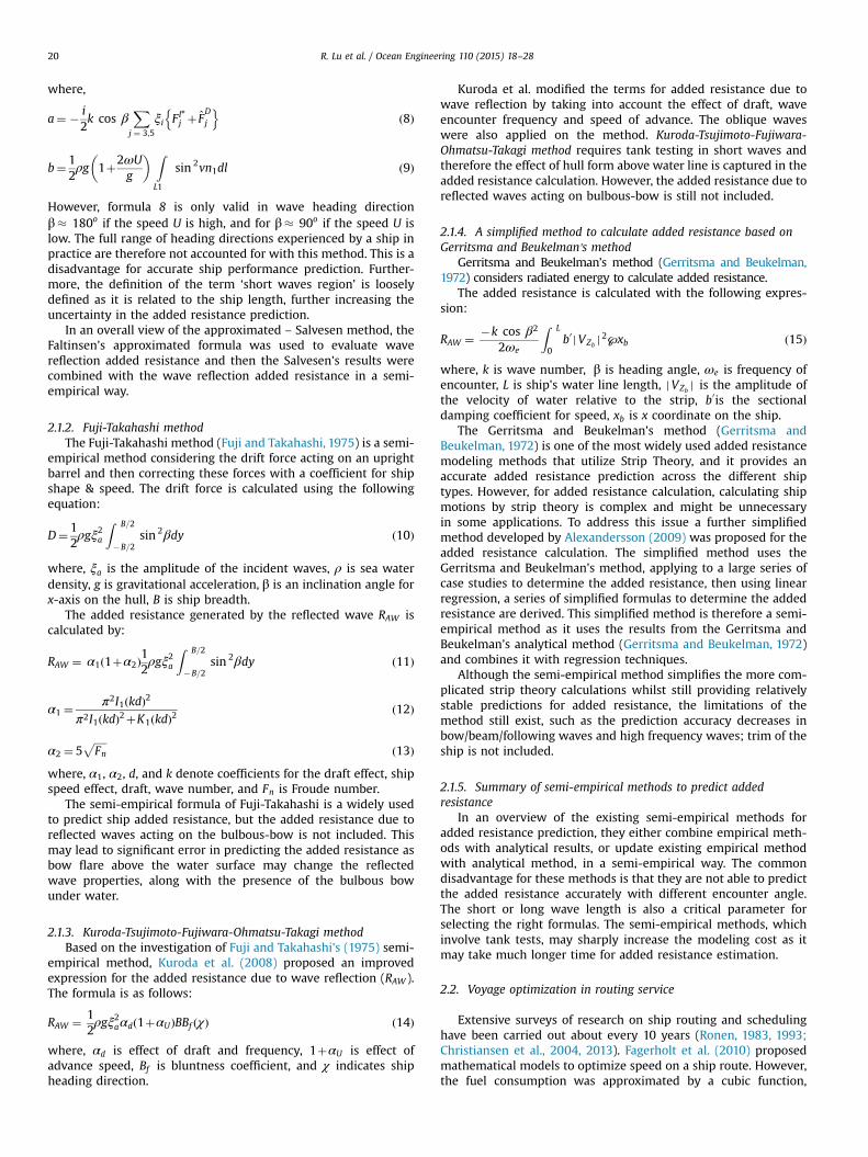
A grid system is able to clearly present the potential routes onship navigation charts. At present, the grid system was plotted onworld map, which is developed using the Google maps API (Googlemaps API, 2015). From start point to destination point, eachpossible route is equally divided into nþ1 legs by n stages; thenodes in one stage are equally distributed with unique longitude.On each stage, the distance between the adjacent nodes is Δx, aspresented in Fig. 4. The number of the stages and the quantity ofnodes in each stage are determined with specific voyage area, totaldistance of route and the availability of computing capacity. Since

Table 4Ship form coefficient Cform due to ship categories and loading condition.

Type of (displacement) ship Ship form coefficient

All ships(except container ships) in loaded loading condition 0.5BNþ BN6:5/(2.7 � Δ2=3)All ships(except container ships) in ballast loading condition 0.7BNþBN6:5/(2.7 � Δ2=3)Container ships in normal loading conditions 0.7BNþBN6:5/(22 � Δ2=3)

R. Lu et al. / Ocean Engineering 110 (2015) 18–28 23

the grids system for specific voyage has been set up, and thedeparture time and ship speeds during each stage are decided byusers, the weather information for the corresponding time atwhich the ship is expected in that area will be downloaded intoeach node by the in house program. Thus the information at eachnode includes its location (latitude and longitude) and the weatherand sea forecast information. The combination of sea direction andship heading direction at two consecutive nodes determines theencounter angle.

5.2. Route selection

As mentioned in Section 1, the user's preferences are incorpo-rated into the development of the decision support system byusing a process of weighting the attributes that are most impor-tant to them (e.g. passage time, fuel consumption). Commonly, theroute with minimum fuel consumption is very popular in routeselection. Based on the grids system, a ship performance modeldeveloped in house is able to predict the total main engine fuelconsumption of each potential route. The outputs of this modelalso include the estimated time of arrival (ETA), sea state, encoun-ter angle, and average speed. At this stage, the development ofautomatic optimization implements in progress. Depending on thepreferences/priorities of shipmasters, such as lowest BN, shortestETA, encounter angle with most head sea and bow sea, or thecombination of these objectives with different weightings, we areable to manually select the route with minimum fuel consumption

considering weather and sea conditions. One case study of theoptimum route selection has been carried out, and the results arepresented in Fig. 10. Based on the grids system presented in Fig. 4,a simulation of the ship performance has been carried out. Thesimulation was run on a typical desktop PC with a 3.4 GHz Intel i7CPU in serial model. With 36 nodes and 30625 potential routes,and the simulation time was around 1.5 h.

6. Results and discussion

6.1. Case studies of semi-empirical ship operational performancemodel

In this study, the ‘Energy Efficiency of Operation’ (EEO) isdefined as the indicator used to illustrate the main engine fuelconsumption efficiency and the ship's operational performance.

EEO¼ FCmcargo � D

ð24Þ

where, FC is the main engine fuel consumption (tonnes), mcargo iscargo carried (tonnes), and D is the distance in nautical milescorresponding to the cargo carried or work done.

An advantage of using the EEO as an indicator is that it containsmany of the same elements and could be easily converted to theEnergy Efficiency Operational Index (EEOI), which is recom-mended within the Ship Energy Efficiency Management Plan(SEEMP) (IMO, 2012).

The basic expression for EEOI for a voyage is defined as:

EEOI ¼P

jFCj � CFj

mcargo � Dð25Þ

Where, j is the fuel type, FCj is the mass of consumed fuel j at onevoyage, and CFj is the fuel mass to CO2 mass conversion factor forfuel j.

In order to verify the accuracy of the semi-empirical shipoperational performance model, the predicted EEO based on themodified Kwon's method and the recorded EEO using recordedoperational data from noon reports were compared in the follow-ing two case studies. The predicted EEO and the recorded EEOwere compared under same conditions, such as Beaufort Number,speed and encounter angle.Fig. 2. Screenshot from decode program, graph of global ocean weather forecast.

Fig. 3. Analysis diagram of the proposed semi-empirical ship operational performance prediction model.

R. Lu et al. / Ocean Engineering 110 (2015) 18–2824

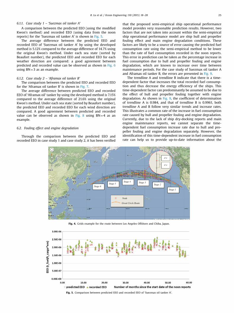
6.1.1. Case study 1 – ‘Suezmax oil tanker A’

A comparison between the predicted EEO (using the modifiedKwon's method) and recorded EEO (using data from the noonreports) for the ‘Suezmax oil tanker A’ is shown in Fig. 5.

The average difference between the predicted EEO andrecorded EEO of ‘Suezmax oil tanker A’ by using the developedmethod is 5.12% compared to the average difference of 14.7% usingthe original Kwon's method. Under each sea state (sorted byBeaufort number), the predicted EEO and recorded EEO for eachweather direction are compared: a good agreement betweenpredicted and recorded value can be observed as shown in Fig. 6using BN¼3 as an example.

6.1.2. Case study 2 – ‘Aframax oil tanker B’The comparison between the predicted EEO and recorded EEO

for the ‘Aframax oil tanker B’ is shown in Fig. 7.The average difference between predicted EEO and recorded

EEO of ‘Aframax oil’ tanker by using the developed method is 7.15%compared to the average difference of 21.6% using the originalKwon's method. Under each sea state (sorted by Beaufort number),the predicted EEO and recorded EEO for each wind direction arecompared. A good agreement between predicted and recordedvalue can be observed as shown in Fig. 8 using BN¼4 as anexample.

6.2. Fouling effect and engine degradation

Through the comparison between the predicted EEO andrecorded EEO in case study 1 and case study 2, it has been verified

that the proposed semi-empirical ship operational performancemodel provides very reasonable prediction results. However, twofactors that are not taken into account within the semi-empiricalship operational performance model are ship hull and propellerfouling effect and main engine degradation conditions. Thesefactors are likely to be a source of error causing the predicted fuelconsumption rate using the semi-empirical method to be lowerthan the rate of fuel consumption recorded in the noon reports.This error in prediction can be taken as the percentage increase infuel consumption due to hull and propeller fouling and enginedegradation, which are known to increase over time betweenmaintenance periods. For the case study of Suezmax oil tanker Aand Aframax oil tanker B, the errors are presented in Fig. 9.

The trendline A and trendline B indicate that there is a time-dependent factor that increases the total recorded fuel consump-tion and thus decrease the energy efficiency of the ships. Thistime-dependent factor can predominantly be assumed to be due tothe effect of hull and propeller fouling together with enginedegradation. As shown in Fig. 9, the coefficient of determinationof trendline A is 0.984, and that of trendline B is 0.9961, bothtrendline A and B follow very similar trends and increase rates.This illustrates a common rate of the increase in fuel consumptionrate caused by hull and propeller fouling and engine degradation.Currently, due to the lack of ship dry-docking reports and mainengine maintenance reports, we cannot separate the time-dependent fuel consumption increase rate due to hull and pro-peller fouling and engine degradation separately. However, theidentification of this time-dependent increase in fuel consumptionrate can help us to provide up-to-date information about the

Stage 6

Δ x

Δ x

Stage 5Stage 4 Stage 3

Stage 2

Stage 1

Node

Great Circle Route

Fig. 4. Grids example for the route between Los Angeles Offshore and Chiba, Japan.

Fig. 5. Comparison between predicted EEO and recorded EEO of ‘Suezmax oil tanker A’.

R. Lu et al. / Ocean Engineering 110 (2015) 18–28 25

Fig. 6. Comparison between predicted EEO and recorded EEO of ‘Suezmax oil tanker A’ with each weather direction under the BN¼3.

Fig. 7. Comparison between predicted EEO and recorded EEO of ‘Aframax oil tanker B’.

Fig. 8. Comparison between predicted EEO and recorded EEO of ‘Aframax oil tanker B’ with each weather direction under the BN¼4.

R. Lu et al. / Ocean Engineering 110 (2015) 18–2826

combined influence on ship performance. The engine data onengine degradation is extremely difficult to obtain and therefore itis a very challenging task to separate the engine degradation andship fouling and remains a future task to develop a separatemodeling.

6.3. Case study of routes selection

With a given departure date and time, draft, fixed averagespeed, specific ship noon reports and sea trial data, the recom-mended route with minimum fuel consumption can be identifiedto the shipmaster as follows (Fig. 10):

� Route a – the blue route is the route with lowest BeaufortNumber (low risk to damage the ship and/or its deck cargo;high comfort to passengers) and low fuel consumption.

� Route b – the green route is the Great-Circle Route – withshortest distance between two ports on earth as well as theroute with shortest time.

� Route c – the violet route is the route with most head sea andbow sea.

� Route d – the brown route is the route with lowest fuelconsumption regardless of voyage time.

� Route e – the red route is the frequently used route as recordedin noon report.

The ship operational performances of these five selected routeshave been compared, as shown in Table 5 by using the developedmodel. The encountered Beaufort Number (BN) and HeadingDirection of each route have been listed. The fuel consumptionof the selected optimum routes can achieve 10% less than therecorded route. As the average voyage speed is fixed, the voyagedurations of the selected optimum routes are very close, but muchless than the recorded route.

7. Conclusion

As the SEEMP is mandatory since 1st January 2013 for all shipsengaged in international trade while at the same time there isfierce competition in shipping market, it is almost a necessity toimprove the existing solutions and approaches for voyageoptimization.

In this paper, a modified Kwon's method has been developed toestimate the ship's added resistance considering the specific shiptype. Based on the modified Kwon's method, as well as ship noonreports and sea trial data, a semi-empirical ship operationalperformance prediction model has been developed to provideaccurate ship operational performance prediction under varyingdrafts, speeds, encounter angles, sea states, fouling effect andengine degradation conditions for each specific ship. Through the

Fig. 9. Error between predicted total fuel consumption of each voyage and recorded one since dry-docking for both Suezmax oil tanker A and Aframax oil tanker B.

Fig. 10. Optimum route selection based on shipmasters' preference.

R. Lu et al. / Ocean Engineering 110 (2015) 18–28 27

two case studies of Suezmax oil tanker A and Aframax oil tanker B,it has been verified that the proposed semi-empirical model isvery fast and very reliable on ship operational performanceprediction, and may also be used to examine the fouling effect ofhull and propeller, and engine degradation trends. Together with agrids system and real-time climatological information, the ships'various courses can be evaluated according to a number ofobjectives including maximization of safety, minimization of fuelconsumption and voyage time. Finally, by utilizing a decisionsupport tool, the shipmasters as well as shore based routeplanners may now select the optimum voyage route with mini-mum fuel consumption considering weather and sea conditions.

8. Future work

Since the weather is stochastic, the ship performance simula-tion needs to be repeated with the weather forecast updatefrequency, which is normally 4 times a day. As the actual voyagecourse may not follow the suggested route absolutely, and thelatest updated weather forecast may not exactly follow previousforecast, minor changes of the suggested route are expected.However, for a long distance voyage, due to the big uncertaintiesof long-term weather forecast, bigger changes may be expected bycomparing the actual voyage route after arrival with the suggestedroute before departure.

It would be interesting to examine the applicability of the semi-empirical ship operational performance prediction model to othership sizes and ship types. Therefore, more case studies will becarried out. Following the development of the ship added resis-tance model, the next step would be the development of a self-refined ship performance database. The database would be able tostore the fuel consumption rate under each sea state, speed,encounter angle, draft and ship conditions (fouling conditions ofhull and propeller, and main engine degradation conditions). Thefeedback from shipmasters would also be recorded to update theship operational performance records. Using the self-refined shipperformance database, the users will be able to extract relevantship operational performance for a given sea state, speed, draft,encounter angle and ship conditions. With the minimum inputs,the improved accuracy in performance prediction will increase thebenefits to be gained from using such systems for energy efficientsolutions.

Acknowledgements

The study presented in this paper was carried out as part of theresearch project: Shipping in Changine Climate - funded by UKResearch Council (EPSRC Grant no. EP/K039253/1).

References

Alexandersson, M., 2009. A study of methods to predict added resistance in waves,performed at seaware AB.

Avgouleas, K., 2008. Optimal Ship Routing Master thesis. Massachusetts Institute ofTechnology http://hdl.handle.net/1721.1/44861.

Bunker Index, IFO 380 price in Port Singapore, Rotterdam and Fujairah. Website:⟨http://www.bunkerindex.com/⟩ (accessed Aug 2014).

Christiansen, M., Fagerholt, K., Ronen, D., 2004. Ship routing and scheduling: statusand perspectives. Transp. Sci. 38 (1), 1–18.

Christiansen, et al., 2013. Ship routing and scheduling in the newmillennium. Eur. J.Oper. Res. 228 (3), 325–333.

Fagerholt, K., Laporte, G., Norstad, I., 2010. Reducing fuel emissions by optimizingspeed on shipping routes. J. Oper. Res. Soc. 61 (3), 523–529.

Faltinsen, O.M., Minsaas, K.J., Liapis, N., Skjordal, S., 1980. Prediction of resistanceand propulsion of a ship in a seaway. In: Proceedings of the 13th ONRSymposium.

Fuji, H., Takahashi, T., 1975. Experimental study on the resistance increase of a shipin regular oblique waves. In: Proceedings of the 14th ITTC, Vol. 4, pp. 351.

Gerritsma, J., Beukelman, W., 1972. Analysis of the resistance increase in waves of afast cargo ship. Int. Shipbuild. Prog. 19 (217), 285–293.

Google maps API. Website: ⟨https://developers.google.com/maps/documentation/javascript/tutorial⟩ (accessed January 2015).

Hinnenthal, J., Clauss, G., 2010. Robust pareto-optimum routing of ships utilisingdeterministic and ensemble weather forecasts. Ships and Offshore Structures. 5,105–114.

Holtrop, J., Mennen, G.G.J., 1982. An approximate power prediction methodInt.Shipbuild. Prog. 29, 166–171.

IMO, 2009. Note by International Maritime Organization. Second IMO GHG Study2009.

IMO, 2011. Note by International Maritime Organization. Amendments to the annexof the protocol of 1997 to amend the International Convention for thePrevention Of Pollution from Ships 1972 as Modified n the protocol of 1978relating thereto (Inclusion of regulations on energy efficiency for ships inMARPOL Annex VI), MEPC 62/24/Add.1, Annex 19.

IMO, 2012. Note by International Maritime Organization. 2012 Guidelines for thedevelopment of a SEEMP, MEPC 63/23, Annex 9.

ITTC, 2011. Note by International Towing Tank Conference. ITTC – RecommendedProcedures – Prediction of Power Increase in Irregular Waves from Model Test,7.5-02-07-02.2.

Kuroda, M., Tsujimoto, M., Fujiwara, T., Ohmatsu, S., Takagi, K., 2008. Investigationon components of added resistance in short waves. J. Jpn. Soc. Nav. Archit.Ocean Eng., 171–176.

Kwon, Y.J., 2008. Speed loss due to added resistance in wind and waves 3,14–16Nav. Archit. 3, 14–16.

Larsson, E., Simonsen, M.H., 2014. Direct Weather Routing. Chalmers University ofTechnology, Master’s thesis http://studentarbeten.chalmers.se/publication/205858-direct-weather-routing.

Matulja, D., Sportelli, M., Guedes Soares, C., PRPIĆ-ORŠIĆ, J., 2011. Estimation ofAdded Resistance of a Ship in Regular Waves Brodogradnja – Shipbuilding.

National Oceanic and Atmospheric Administration (NOAA) Website: ⟨www.noaa.gov⟩ (accessed June 2015).

Padhy, C.P., Sen, D., Bhaskaran, P.K., 2008. Application of wave model for weatherrouting of ships in the north indian ocean. Nat. Hazards 44, 373–385.

Ronen, D., 1983. Cargo ships routing and scheduling: surveys of models andproblems. Eur. J. Oper. Res. 12 (2), 183–192.

Ronen, D., 1993. Ship scheduling: the last decade. Eur. J. Oper. Res. 71 (3), 325–333.Salvesen, N., 1978. Added resistance of ships in waves. J. Hydronaut 12 (1), 24–34.Shao, W., 2013. Development of an intelligent tool for energy efficient and low

environment impact shipping. University of Strathclyde, Ph.D thesis (PrimoLocal Repository).

Wang, X., Teo, C., 2013. Integrated hedging and network planning for containershipping’s bunker fuel management. Marit. Econ. Logist., 172–196.

Table 5Comparison of ship operational performance between the selected optimum routes and recorded route.

The encountered Beaufort Number(BN), Heading Direction with givendeparture date & time, loadingcondition and fixed average speed

Route a Route b Route c Route d Route e

BN Direction BN Direction BN Direction BN Direction BN Direction5 Bow 5 Bow 5 Head 5 Bow 5 Bow5 Beam 5 Beam 5 Bow 5 Beam 7 Bow3 Bow 4 Bow 5 Bow 3 Bow 6 Head3 Beam 3 Beam 4 Beam 3 Beam 5 Head3 Beam 4 Beam 4 Beam 3 Beam 5 Head3 Beam 3 Beam 4 Bow 3 Beam 5 Head1 Head 1 Head 2 Head 1 Head 2 Bow

Voyage Duration (h) 367.7 366.1 368.5 367.3 392Main Engine Fuel Consumption (t) 555.5 558.3 580.4 554.9 623.5% of Fuel saving compared to Route e 10.90 10.46 6.91 11.01 0

R. Lu et al. / Ocean Engineering 110 (2015) 18–2828