A

Scalable Multiphysics Network Simulation Using PETSc DMNetwork

DANIEL A. MALDONADO, Argonne National LaboratorySHRIRANG ABHYANKAR, Argonne National LaboratoryBARRY SMITH, Argonne National LaboratoryHONG ZHANG, Argonne National Laboratory

A scientific framework for simulations of large-scale networks, such as is required for the analysis of criticalinfrastructure interaction and interdependencies, is needed for applications on exascale computers. Such aframework must be able to manage heterogeneous physics and unstructured topology, and must be reusable.To this end we have developed DMNetwork, a class in PETSc that provides data and topology managementand migration for network problems, along with multiphysics solvers to exploit the problem structure. Iteases the application development cycle by providing the necessary infrastructure through simple abstrac-tions to define and query the network. This paper presents the design of the DMNetwork, illustrates its userinterface, and demonstrates its ability to solve large network problems through the numerical simulationof a water pipe network with more than 2 billion variables on extreme-scale computers using up to 30,000processor cores.

Additional Key Words and Phrases: Networks, multiphysics, extreme-scale computing

1. INTRODUCTIONModeling, simulation, and analysis of critical infrastructures—assets providing es-sential services that form the backbone of a nation’s health, security, and economyincluding power distribution systems, water distribution, gas distribution, communi-cations, and transportation—are of paramount importance from several strategicallyimportant perspectives, including maintaining sustainability, security, and resiliencyand providing key insights for driving policy decisions. The Critical InfrastructuresAct [Dominici 2001] defines critical infrastructures as “systems and assets, whetherphysical or virtual, so vital that the incapacity or destruction of such systems and as-sets would have a debilitating impact on security, national economic security, nationalpublic health or safety, or any combination of those matters.” Such infrastructurescomprise a large-scale network of assets spawned over wide geographical regions.

From the modeling and simulation standpoint, these critical infrastructures pose amultiphysics problem on an unstructured network with problem sizes from millionsto billions of variables. Their analysis is computationally challenging because of theneed for managing unstructured topology and heterogeneous node-edge characteris-tics. Several software packages assist scientists and engineers in modeling complexmultiphysics networked problems (e.g., Simulink R© [Mathworks 2017], Modelica [As-sociation 2017], and LabView [Instruments 2017]), yet the problems they are able tosolve are restricted by size. EPANET, a software for simulating water distribution pip-ing systems [Rossman 2000] is a particular example of network simulation tool thatcan be implemented using our tools. For the scaling studies in this paper we incor-porate a simple model of such a distribution system. Our work is not directly relatedto network analysis packages, —such as, SNAP [Leskovec and Sosic 2016], NetworkX[Hagberg et al. 2008], and NetworKit [Team 2017], —that do not provide simulationcapability. Nor is it related to domain specific simulators such as the packet-level simu-lations modeling the transmission in a computer communication network in [Fujimotoet al. 2003] or the internet simulator NS-3 [Wehrle et al. 2010, p. 15–34].

Exascale computing provides opportunities and challenges for simulating such com-plex networked systems [Brase and Brown 2009]. In problems arising from fields asdiverse as power distribution systems, water distribution, gas distribution, commu-

A:2 D. A. Maldonado et al.

nications, and transportation, a common mathematical structure exists that can beexploited [Jansen and Tischendorf 2014] to develop scalable tools for multiphysics net-work simulation.

In this paper, we present a new package, DMNetwork, for modeling and simula-tion of multiphysics networks designed for exascale computers. DMNetwork providesthe underlying infrastructure for managing the topology and the physics for large-scale networks. It is designed to scale for large networks while facilitating easy andrapid development of network applications. DMNetwork is seamlessly integrated inthe Portable Extensible Toolkit for Scientific Computing (PETSc) [Balay et al. 2016],thus allowing the usage of the solvers available in PETSc. The name DMNetworkcomes from the PETSc base class DM, that provides interfaces between the PETSctime-integrators and algebraic solvers and problem specific representations of mathe-matical models. For example, the PETSc DMDA class provides the connection betweenpartial differential equation models on structured grids and the PETSc solvers.

2. NETWORKS, PHYSICS AND SOLVERSConsider a series of physical elements (water pipes, gas pipes, power transmissionlines) that are connected via junctions to form a network or a network of networks.Our paper presents abstractions that allow users to express their problem concisely,hide cumbersome data management operations, and use flexible and efficient solvers.The abstractions provide several convenient ways for networked system compositionand decomposition, including the following.

(1) Domain decomposition [Smith and Tu 2013]: Decomposition of a computational do-main into smaller subdomains. Each subnetwork is defined by a subregion of theentire region on which the original network is defined, as illustrated in Fig. 1.

(2) Fieldsplit [Brown et al. 2012; Smith et al. 2012]: Splitting of a multiphysics systeminto multiple single physics subsystems. Figure 2 shows a network composed of twosubnetworks that represent distinct physics (e.g., electrical and water distribution).

(3) Multilevel domain decomposition and fieldsplit: Combination of domain decomposi-tion and fieldsplit, as shown in Fig. 3.

Fig. 1. A network is partitioned into two subnetworks, with regard to its topology..

In DMNetwork, to construct a network or a composite network, we add a series ofphysical elements, for example, water pipes, gas pipes, and power transmission linesas the edges of the graph, and pipe junctions, electrical generators and load systems

Scalable Multiphysics Network Simulation Using PETSc DMNetwork A:3

Fig. 2. A network, composed by two subnetworks of distinct physics (represented by solid and dashed lines)(e.g., electrical and water distribution). Customized solvers can be applied to the individual subnetwork.

.

Fig. 3. A multilevel domain decomposition and fieldsplit solver can be used to solve this mixed case..

as the vertices of the graph. From this information DMNetwork builds a mathemat-ical model for the entire physical system. The model is generally either a nonlinearalgebraic equation or a differential algebraic equation (DAE). The Jacobian operatorof such system often has the following structure:

N =

P1 . . . C1

P2 . . . C2

P3 . . . C3

......

.... . .

...D1 D2 D3 . . . J

, (1)

where the submatrices Pi represent individual elements of the network: a water pipeor a power transmission line, a water reservoir or an electrical generator. These ele-ments can have dissimilar structures and time scales. For instance, in power systemseach vertex represents a mechanical generator that produces electrical energy, eachof which will have different parameters and even different equations. In water net-works, the edges represent water conduits modeled with partial differential equations,whereas the vertices represent either simple boundary conditions of pressure and flow

A:4 D. A. Maldonado et al.

or complex mechanical regulators such as valves or variable height reservoirs. Fur-thermore, their physical meaning is independent from the network. The matrices J ,Ci, and Di contain information about boundary conditions of the individual systemssystem, such as continuity or energy conservation; that is, they provide constraints forsystems Pi. They also provide information about the topological structure of the system(what is connected to what). The PETSc fieldsplit preconditioner can take advantageof this structure by employing customized preconditioners for each Pi.

Consider three coupled networks. We can write

N =

N1 C1

N2 C2

N3 C3

D1 D2 D3 J

, (2)

where J is the intersection network (e.g., overlapping elements in Fig. 1) andN1, N2, N3

have the same structure as N in Equation (1). Domain decomposition preconditioners,such as block Jacobi and the overlapping additive Schwarz method [Balay et al. 2016],are amenable to parallel execution utilizing this structure. Depending on the networkphysics, it can be modeled by using a set of linear algebraic equations, a set of nonlinearequations, or a set of time-dependent equations. The PETSc library provides threelayers of solvers: KSP, SNES, and TS, as illustrated in Table I, to solve these problems,respectively.

Table I. PETSc Solvers

Solver Name Description Mathematical FormKSP and PC Krylov subspace solvers and preconditioners Ax− b = 0

SNES Non-linear solvers F (x) = 0TS Time stepping solvers F (t, x, x) = 0

DMNetwork is compatible with these solvers and provides a set of directives to helpusers set up their problem. As an example, consider a nonlinear system F (x) = 0. WithNewton’s method, we can find a sequence of approximations:

J(xk)∆xk = −F (xk), xk+1 = xk + ∆xk. (3)We obtain each iterate by evaluating F (xk) (residual function) and J(xk) (Jacobian)and solving Equation (3) iteratively to obtain the approximated solution xk. For a largesystem comprising equations of different nature and different parameters, building themodel requires the following tasks:

— Create problem specific data structures to distribute the parameters across the com-puter processors.

— Calculate the dimension of Jacobian matrix J , and preallocate J (determine thenon-zero pattern of the sparse matrix).

— Evaluate the residual function and Jacobian for the given parameters.

With DMNetwork, the process is greatly simplified. The user needs to provide thenumber of degrees of freedom for each edge and vertex. Then DMNetwork takes careof the parallel distribution, preallocation, partitioning, and setting up of needed datastructures to allow utilizing user-provided function evaluation routines. The user func-tion merely needs to iterate by edges and vertices, retrieve the problem specific dataand variables associated with them, and perform the local portion of the function eval-uation based on their local mathematical models. PETSc also provides some tools tohelp approximate the Jacobian matrices efficiently via finite differences with coloring(discussed in the next section).

Scalable Multiphysics Network Simulation Using PETSc DMNetwork A:5

3. SOFTWARE STRUCTURE AND INTERFACEIn the preceding section we showed that the systems of equations arising from net-work problems present some mathematical structure amenable to parallelization. Fur-thermore, given that each subsystem of equations can present different physics ormathematical structure, supporting the use of different solvers for each subsystem isnecessary. Since its inception, PETSc was meant to provide an environment for test-ing various solver options, particularly linear Krylov methods and the preconditionersthey use, with minimal coding effort from the user. The user can often switch betweensolvers with runtime options.

DMPlex is a class in PETSc to handle general unstructured meshes, the mathemat-ical models on the meshes and their connection to the PETSc solvers. [Lange et al.2016]. DMNetwork is a recently developed subclass of DMPlex that provides specificabstractions for general networks. Both the vertices and edges can represent any num-ber of physical models. New vertices and edges can be easily inserted through an API,and the existing ones can be removed or updated with minimum local changes. On mul-tiple processors, DMNetwork can partition the network using the graph partitioningpackages, such as ParMetis [Karypis et al. 2005] or Chaco [Hendrickson and Leland1995], and distribute the problem specific data describing the physics to the appropri-ate processors.

3.1. DMNetwork Object and Its InterfaceThe DMNetwork object contains topological information about the problem as well asphysical modeling data. In this section, we illustrate the DMNetwork interface. Firstwe create a DMNetwork object. Users create their own problem specific data struc-tures, based on C structs, that contain data associated to the physics occurring in thevertices and edges (for example, in the edge data structure, the user may include theelectrical resistance of the circuit). These problem specific data structures are regis-tered as components that can be accessed later via DMNetwork.

1 PetscInt VERTEX, EDGE; /∗ keys for the two models ∗ /2 typedef struct vertex Vertex ;3 typedef struct edge Edge ;4 DMNetworkCreate (PETSC COMM WORLD,&dmnetwork ) ;5 DMNetworkRegisterComponent ( dmnetwork , ” vertex ” , s i z e o f ( Vertex ) ,&VERTEX) ;6 DMNetworkRegisterComponent ( dmnetwork , ” edge ” , s i z e o f ( Edge ) ,&EDGE) ;

In this simple example, we have only two problem specific data structures, one foredges and one for vertices. In realistic simulations there are almost always more thantwo types.

Next, we provide the DMNetwork with information about the topology of the prob-lem: the local number of vertices, the number of edges, and a list of the connectivity ofthe edges.

1 DMNetworkSetSizes ( dmnetwork , nvertex , nedge ,PETSC DETERMINE,PETSC DETERMINE) ;2 DMNetworkSetEdgeList ( dmnetwork , edge l i s t ) ;3 DMNetworkLayoutSetUp( dmnetwork ) ;

In the final function call the DMNetwork creates a preliminary internal representationof the graph defined by the network. Edges and vertices each are assigned to a uniqueprocess. We can access the range of edges and vertices on the process, and add theproblem-specific data parameters and the number of degrees of freedom for each entity.

1 DMNetworkGetEdgeRange ( dmnetwork,&eStart ,&eEnd) ;2 f o r ( i = eStart ; i < eEnd ; i ++) {3 DMNetworkAddComponent( dmnetwork , i ,EDGE,&edge [ i−eStart ] )4 DMNetworkAddNumVariables ( dmnetwork , i , nvar ) ;5 }

A:6 D. A. Maldonado et al.

1 DMNetworkGetVertexRange ( dmnetwork,&vStart ,&vEnd) ;2 f o r ( i = vStart ; i < vEnd ; i ++) {3 DMNetworkAddComponent( dmnetwork , i ,VERTEX,&vertex [ i−vStart ] ) ;4 DMNetworkAddNumVariables ( dmnetwork , i , nvar )5 }

The network then is partitioned and distributed to multiple processors to approxi-mately equalize the number of unknowns per process.

1 DMSetUp( dmnetwork ) ;2 DMNetworkDistribute(&dmnetwork , 0 ) ;

With these steps the user has created a distributed network object that contains thefollowing:

— A (partitioned) graph representation of the problem— A data structure containing needed ghost vertices and communication data struc-

tures needed to update the ghost values— Memory space for the unknowns in each vertex and edge— Physical data in each vertex and edge, related to the model for that entity— Preallocation of the (Jacobian) matrices, that is, the determination of the nonzero

structure of the matrix based on the graph.

Whether the user wants to solve the problem using a linear solver, a nonlinear solver,or a time-integrator, this DMNetwork object facilitates both the evaluation of the resid-ual function (or right-hand side vector for linear problems), and computation of the(Jacobian) matrix.

3.2. A Example: Electric CircuitWe will solve a toy linear electric circuit problem from [Strang 2007]. The topologyof the electrical circuit is shown in Fig. 4. The circuit must obey the Kirchhoff laws.Hence, in the vertices of the graph, the energy is not accumulated:∑

j

i(j) − isource(k) = 0 , (4)

where i(j) is the current flowing though the branch (edge) j, incident to the node k. Theisource(k) allows one to account for current sources at node k. The voltage drop across theedge k, from v(i) to v(j), is defined by Ohm’s law plus any existing voltage source v(k)source:

i(k)

r(k)+ v(j) − v(i) − v

(k)source = 0 . (5)

We use the superscript and subscript to distinguish between edge and vertex quanti-ties, respectively. In this case i(∗) is an edge variable, and v(∗) is a vertex variable.

These equations, as Strang[2007] shows, can be represented with the KKT matrixand the graph Laplacian. This structure is shared by many network flow problems,such as water networks: [

R−1 AAT

] [iv

]=

[vsourceisource

]. (6)

The practical implementation of this problem requires knowing the topology or con-nectivity of the network (a list of vertices and a list of edges defined by vertex pairs)and the physics (resistance, values of voltage source, and current source).

Scalable Multiphysics Network Simulation Using PETSc DMNetwork A:7

Fig. 4. Network diagram. Resistances are represented by zig-zag lines (R), voltage sources by parallel lines(V ), and current sources by an arrow (I). The vertices of the graph are potentials, and the current flowsacross the edges.

.

3.3. Residual FunctionThe following is a code fragment from petsc/src/ksp/ksp/examples/tutorials/net-work/ex1.c [Balay et al. 2016]. It illustrates how to access DMNetwork information,iterate over the graph structure, and define the numerical problem that must be solvedby computing the matrix and right-hand side vector for the linear system.

1 PetscErrorCode FormOperator (DM dmnetwork , Mat A, Vec b )2 {3 DMNetworkGetComponentDataArray ( dmnetwork,&arr ) ;4 DMNetworkGetEdgeRange ( dmnetwork,&eStart ,&eEnd) ;5 DMNetworkGetVertexRange ( dmnetwork,&vStart ,&vEnd) ;

The array arr contains the physical data we provided in theDMNetworkAddComponent(). In order to achieve high performance, this problemspecific data is stored and managed by DMNetwork in a simple one-dimensionalarray, as opposed to using pointers to a collection of C structs or C++ classes. Thus weaccess the correct data for a given entity through a variable offset that DMNetworkprovides (shown below). We considered using a higher-level iterator construct toloop over the entities; but based on many years of experience with unstructuredmesh codes, we have concluded that simple, basic data structures provide higherperformance and a simplicity of debugging that is more important than the slightlysimpler code syntax one can obtain with iterators. Of course developers are free tolayer an iterator abstraction of their liking directly on top of the DMNetwork interfaceif they value the syntax it offers.

The construction of the matrix and right-hand side vector can be implemented withthe following code:

1 f o r ( e = eStart ; e < eEnd ; e++) {2 DMNetworkGetComponentTypeOffset ( dmnetwork , e ,0 ,NULL,&compoffset ) ;3 DMNetworkGetVariableOffset ( dmnetwork , e,& l o f s t ) ;4 DMNetworkGetConnectedNodes ( dmnetwork , e,&cone ) ;5 DMNetworkGetVariableOffset ( dmnetwork , cone [0] ,& l o f s t f r ) ;6 DMNetworkGetVariableOffset ( dmnetwork , cone [1] ,& l o f s t t o ) ;7

8 branch = ( Branch∗ ) ( arr + compoffset ) ;9 barr [ l o f s t ] = branch−>bat ; /∗ battery value ∗ /

10

11 row [ 0 ] = l o f s t ;12 co l [ 0 ] = l o f s t ; val [ 0 ] = 1 ;13 co l [ 1 ] = l o f s t t o ; val [ 1 ] = 1 ;14 co l [ 2 ] = l o f s t f r ; val [ 2 ] = −1;

A:8 D. A. Maldonado et al.

15 MatSetValuesLocal (A,1 , row ,3 , col , val ,ADD VALUES) ;16

17 /∗ from node ∗ /18 DMNetworkGetComponentTypeOffset ( dmnetwork , cone [ 0 ] , 0 ,NULL,&compoffset ) ;19 node = (Node∗ ) ( arr + compoffset ) ;20

21 i f ( ! node−>gr ) { /∗ not a boundary node ∗ /22 row [ 0 ] = l o f s t f r ;23 co l [ 0 ] = l o f s t ; val [ 0 ] = −1;24 MatSetValuesLocal (A,1 , row ,1 , col , val ,ADD VALUES) ;25 }26

27 /∗ to node ∗ /28 DMNetworkGetComponentTypeOffset ( dmnetwork , cone [ 1 ] , 0 ,NULL,&compoffset ) ;29 node = (Node∗ ) ( arr + compoffset ) ;30

31 i f ( ! node−>gr ) { /∗ not a boundary node ∗ /32 row [ 0 ] = l o f s t t o ;33 co l [ 0 ] = l o f s t ; val [ 0 ] = 1 ;34 MatSetValuesLocal (A,1 , row ,1 , col , val ,ADD VALUES) ;35 }36 }37 f o r ( v = vStart ; v < vEnd ; v++) {38 DMNetworkIsGhostVertex ( dmnetwork , v,&ghost ) ;39 i f ( ! ghost ) {40 DMNetworkGetComponentTypeOffset ( dmnetwork , v ,0 ,NULL,&compoffset ) ;41 DMNetworkGetVariableOffset ( dmnetwork , v,& l o f s t ) ;42 node = (Node∗ ) ( arr + compoffset ) ;43

44 i f ( node−>gr ) {45 row [ 0 ] = l o f s t ;46 co l [ 0 ] = l o f s t ; val [ 0 ] = 1 ;47 MatSetValuesLocal (A,1 , row ,1 , col , val ,ADD VALUES) ;48 } e lse {49 barr [ l o f s t ] += node−>i n j ;50 }51 }52 }

First we iterate over the edges (Line 1). For each edge we retrieve the componentoffset (that is, a pointer to the problem specific data for this edge), the edge variableoffset, and the offsets for the variables in the boundary vertices (Lines 2–6). Next wewrite the Kirchhoff voltage law (Lines 11–15); and then, for each boundary vertex,we check whether the vertex is not a ghost value and write its contribution to theKirchhoff current law (Lines 18–36). We then iterate over each vertex and add thecontribution of each current injection to the corresponding equation.

3.4. Finite-Difference Jacobian Approximation with ColoringIn the engineering fields, from which many of the network problems arise, the mod-els often have a complicated structure: they may include control logic and react ina discrete way to transients in the network. Writing an analytical Jacobian matrixevaluation subroutine is a daunting, time-consuming, and error-prone task. PETSc of-fers tools to calculate a finite-difference approximation of the Jacobian matrix suitablefor some classes of problems. DMNetwork contains information about the connectivityof the vertices and edges, which enables building a sparse Jacobian matrix structureand using matrix coloring schemes [Coleman and More 1983] for efficient Jacobianevaluation. We have designed and implemented a customized, scalable matrix color-ing routine for networks that minimizes the number of colors required and thus onlyincurs a small amount of interprocessor data communication. We also allow the input

Scalable Multiphysics Network Simulation Using PETSc DMNetwork A:9

of problem-specific information to reduce memory needs by using user-provided sparsematrix nonzero structures for individual edges and vertices:

1 DMNetworkEdgeSetMatrix ( dmnetwork , e , Juser ) ;2 DMNetworkVertexSetMatrix ( dmnetwork , v , Juser ) ;

The finite-difference Jacobian approximation with coloring for networked applica-tions then involves the following steps:

(1) User provides subroutine for local function evaluation.(2) User provides the problem specific sparse matrix nonzero structures for the individ-

ual edges and vertices; if none are provided, dense matrix subblocks are used.(3) DMNetwork builds the global sparse Jacobian matrix structure based on the global

network topology and problem specific sparse matrix nonzero structures (when pro-vided).

(4) Jacobian matrix is computed by finite-difference approximation using a matrix col-oring scheme in an efficient and scalable fashion.

We present numerical experiments in Sec. 4.4 to demonstrate that this Jacobianapproximation can be highly efficient and scalable on extreme-scale computers.

4. HYDRAULIC TRANSIENT SIMULATION ON EXTREME-SCALE COMPUTERSHydraulic transient simulations are performed for problems such as water distribu-tion, oil distribution, and hydraulic generation. In this paper we focus on the simu-lation of water transients on closed conduits such as an urban distribution system.Simulation of hydraulic transients involves the calculation of pressure changes in-duced by a sudden change of velocity of the fluid [Chaudhry 1979; Wylie and Streeter1978]. These velocity changes create a pressure wave that propagates proportionallyto the speed of sound in the fluid media and the friction of the conduits. The modelingof this problem involves the solution of a set of PDEs. The disturbance of the systemis introduced through a perturbation on the boundary conditions and results in a stiffdifferential equation, traditionally solved through the method of characteristics.

4.1. Description of the ProblemTo facilitate discussion, we introduce the following notation:

nv, ne: number of junctions (vertices) and pipes (edges) of the network;Qk, Hk: water flow and pressure for pipe k;Qi, Hi: boundary values of water flow and pressure adjacent to junction i;nei: number of connected pipes at junction i.

For pipe k, the water flow and pressure are described by the momentum and conti-nuity equations:

∂Qk

∂t+ gA

∂Hk

∂x+RQk

∣∣Qk∣∣ = 0 , (7)

gA∂Hk

∂t+ a2

∂Qk

∂x= 0 , (8)

where g is the gravity constant, A is the area of the conduit, R = f2DA with f being the

friction of the conduit and D its diameter, and a the velocity of the pressure wave in

A:10 D. A. Maldonado et al.

the conduit. At an interior junction i, nei > 1, the boundary conditions satisfynei∑j=1

Qkj

i = 0 , (9)

Hkj

i −Hk1i = 0, j = 2 . . . nei . (10)

Equations (7)–(10) are built over a network or a network of subnetworks. Note thatthe physical meaning of these equations corresponds to conservation of energy andmass. Special boundaries such as the connection to a reservoir, valve, or pump provideapplication-specific boundary conditions.

4.2. Steady StateSystems engineers customarily divide the simulation of a dynamic system into twostages: steady state and transient state. Most systems are assumed to operate insteady-state conditions until some disturbance perturbs the system. In steady statethe magnitudes do not vary with time. Thus Equations (7)–(8) are reduced to

gA∂Hk

∂x+RQk

∣∣Qk∣∣ = 0 , (11)

∂Qk

∂x= 0 . (12)

We can make two assertions for steady state: (1) along an individual pipe, the flowQk is constant; and (2) the drop of pressure Hk can be described with a linear func-tion. Hence values (Q, H) inside a pipe can be uniquely determined by their bound-ary values, which satisfy the interior junction equations (9)–(10) and special boundaryconditions. Equations (9) and (10) represent global connectivity of the network. Addingspecial boundary conditions, they form an algebraic differential subsystem that we callthe junction subsystem. We name the rest of system the pipe subsystem. The junctionsubsystem has an ill-conditioned Jacobian matrix in general; its size is determined bythe numbers of vertices, edges, and the network layout but is independent of the levelof refinement used within the pipes for the differential equations (11)–(12). Thus itforms a small, but difficult to solve, subsystem requiring strong preconditioner for itssolution.

The Newton-Krylov method [Kelley 2003] is used to solve the nonlinear steady stateproblem. For its linear iterations, we use the FieldSplit preconditioner to extract thejunction equations from entire system, apply a direct linear solver (e.g., MUMPS paral-lel LU solver [Amestoy et al. 2001]), and use block Jacobi with ILU(0) in each subblockof the Jacobian for the rest of the system. The command-line options for this executionare as follows.

Preconditioner for entire system:

-initsol_pc_type fieldsplit

Preconditioner for junction subsystem:

-initsol_fieldsplit_junction_pc_type lu-initsol_fieldsplit_junction_pc_factor_mat_solver_package mumps

Preconditioner for pipe subsystem:

-initsol_fieldsplit_pipe_pc_type bjacobi

Scalable Multiphysics Network Simulation Using PETSc DMNetwork A:11

-initsol_fieldsplit_pipe_sub_pc_type ilu

The prefix initsol is used to distinguish the steady-state system from the transientsystem, which is solved next. In Table II we compare the performance and strong scal-ability of the LU and FieldSplit preconditioners for a single network with 3,949,792variables on Edison, a Cray XC30 system (see Sec. 4.4). Most of the time is spent inthe LU factorization. Hence when we use FieldSplit employing block Jacobi on thelarger subdomain, computation time is greatly reduced.

Table II. Comparison of LU and FieldSplit Preconditioners

No. of SNES Solution Time (sec) KSP Solution Time (sec)Cores LU FieldSplit LU FieldSplit

24 52.0 3.91 49.1 1.1048 45.9 3.84 43.0 0.9372 42.3 2.92 41.0 0.67

The steady state solution was compared with the EPANET software using a bench-mark case from [de Corte and Sorensen 2014] consisting on 74 junctions, 102 pipesand one reservoir. The solution of the problem was consistent with EPANET’s solu-tion, minding the differences in the approach.

4.3. Transient StateIn the transient state we calculate the pressure wave that arises after a perturbationis applied to the steady state solution. We solve Equations (7)-(10), which are a set ofhyperbolic partial differential and algebraic equations. We have simulated a case ap-pearing in [Wylie and Streeter 1978, p. 38] to benchmark the accuracy of our solution.The case consists on a single pipe connected to a reservoir and a valve. At time t = 0+

the valve is closed instantaneously, creating a pressure wave that propagates throughthe pipe back and forward. In Fig. 5, we plot the pressure profiles (hydraulic or piezo-metric head, in water column meters) for a set of equally spaced points along the waterpipe. In particular, the dark blue curve in the figure represents the pressure at the wa-ter reservoir. The water reservoir is treated as a constant pressure source, and hencethe pressure is constant through time. On the other extreme, in light blue, we cansee the pressure wave next to the valve, which sharply increases after its closure. Thepoint right next to the valve (in yellow) will not be perturbed until the pressure wavehas reached it, at a time that is proportional to the speed of the wave. This examplegives us a physical intuition of the importance of the Courant number in computing hy-perbolic PDEs. Several methods to solve such systems are employed in the literature.In this section we describe two of the most common ones.

4.3.1. Method of characteristics. The method of characteristics [Chaudhry 2014] involvesapplying a change of variables to Equations (7)–(8). Taking (8), scaling it by a term λ,and adding it to (7), we obtain

(∂Qk

∂t+ λa2

∂Qk

∂x) + λgA(

∂Hk

∂t+

1

λ

∂Hk

∂x) +RQk

∣∣Qk∣∣ = 0 . (13)

Using the chain rule, we obtain

dQ

dt=∂Q

∂t+∂Q

∂x

dx

dt, (14)

A:12 D. A. Maldonado et al.

Fig. 5. Pressure wave on a conduit. This pressure wave is created in a single pipe with a conduit, whenthe end of the conduit is instantaneously closed. The vertical axis measures the piezometric head in watercolumn meters, and each different color shows the pressure of a point in the pipe.

.

anddH

dt=∂H

∂t+∂H

∂x

dx

dt. (15)

By defining1

λ=dx

dt= λa2 , (16)

that is λ = ± 1a , we obtain the ODEs in which the independent variable x has been

eliminated:∂Q

∂t± gA

a

∂H

∂t+RQ |Q| = 0 . (17)

4.3.2. Lax scheme. An alternative to the method of characteristics is the Lax scheme[Chaudhry 2014], an explicit first-order scheme. We approximate the partial deriva-tives as

∂H

∂t=Hj+1

i − Hi

∆t,

∂Q

∂t=Qj+1

i − Qi

∆t, (18)

∂H

∂x=Hj

i+1 −Hji−1

2∆x,

∂Q

∂x=Qj

i+1 −Qji−1

2∆x, (19)

Hi = 0.5(Hji−1 +Hj

i+1), Qi = 0.5(Qji−1 +Qj

i+1) . (20)

These equations are applicable only to interior points; hence we use the characteristicequations at the boundaries.

4.4. Experimental ResultsWe conducted experiments on two computer systems: Cetus, an IBM Blue Gene/Q su-percomputer in the Argonne Leadership Computing Facility [ALCF 2017], and Edison,

Scalable Multiphysics Network Simulation Using PETSc DMNetwork A:13

a Cray XC30 system in the National Energy Research Scientific Computing Center[NERSC 2017]. Cetus has 4,096 nodes, each with 16 1600 MHz PowerPC A2 cores with16 GB RAM per node, resulting in a total of 65,536 cores. Edison has 5,576 computenodes. A node has 64 GB memory and two sockets, each with a 12-core Intel processorat 2.4 GHz, giving a total of 133,824 cores.

Fig. 6. Water network provided by [de Corte and Sorensen 2014]..

Our test network was obtained from [de Corte and Sorensen 2014] in EPANET for-mat [Rossman 2000]. It consists of 926 vertices and 1,109 edges of various lengths (seeFig. 6). Equations (7)–(10) were discretized via the finite volume method into a sys-tem over this single network with a total of 3,949,792 variables. We call the resultingDMNetwork sub-dmnetwork.

We then built a large network by duplicating sub-dmnetwork and composing theminto a composite dmnetwork. Artificial edges were added between the sub-dmnetworkswithout introducing new variables over these edges. To perform weak-scaling studiesof the simulation when the number of sub-dmneworks was doubled, we increase thenumber of processor cores proportionally.

The focus of our simulation is the time integration of the transient-state system,with its initial solution computed from the steady-state system (11)–(12). All the ex-periments were done by using the PETSc DAE solver, that is, the Lax scheme for eachpipe and backward Euler time integration for the entire composite network system(7)–(10). The Jacobian matrix was approximated by finite differencing with coloring,as discussed in Sec. 3.4, and the Krylov GMRES iterations with selected precondi-tioner were implemented for the linear solves. Since the Jacobian matrix structuredoes not change with the time, the computing time spent at each time step remainsapproximately constant. We run only 10 time steps for each test case.

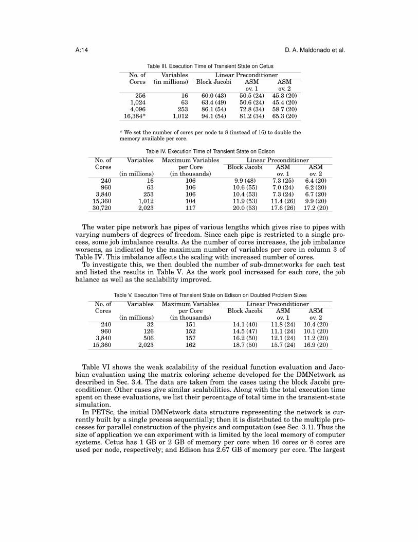
Tables III and IV show the scalability of the simulation on Cetus and Edison. Thelinear solvers dominate the computation with efficiency determined by the selectedpreconditioners. Among all the preconditioners provided by PETSc, we found the blockJacobi and the additive Schwarz method (ASM) with subdomain overlapping 1 (ov.1)and 2 (ov.2) to be the most efficient for our application. In the tables, we compare thesethree preconditioners using the total simulation time and cumulative number of lineariterations (given in parentheses).

A:14 D. A. Maldonado et al.

Table III. Execution Time of Transient State on Cetus

No. of Variables Linear PreconditionerCores (in millions) Block Jacobi ASM ASM

ov. 1 ov. 2256 16 60.0 (43) 50.5 (24) 45.3 (20)

1,024 63 63.4 (49) 50.6 (24) 45.4 (20)4,096 253 86.1 (54) 72.8 (34) 58.7 (20)

16,384* 1,012 94.1 (54) 81.2 (34) 65.3 (20)

* We set the number of cores per node to 8 (instead of 16) to double thememory available per core.

Table IV. Execution Time of Transient State on Edison

No. of Variables Maximum Variables Linear PreconditionerCores per Core Block Jacobi ASM ASM

(in millions) (in thousands) ov. 1 ov. 2240 16 106 9.9 (48) 7.3 (25) 6.4 (20)960 63 106 10.6 (55) 7.0 (24) 6.2 (20)

3,840 253 106 10.4 (53) 7.3 (24) 6.7 (20)15,360 1,012 104 11.9 (53) 11.4 (26) 9.9 (20)30,720 2,023 117 20.0 (53) 17.6 (26) 17.2 (20)

The water pipe network has pipes of various lengths which gives rise to pipes withvarying numbers of degrees of freedom. Since each pipe is restricted to a single pro-cess, some job imbalance results. As the number of cores increases, the job imbalanceworsens, as indicated by the maximum number of variables per core in column 3 ofTable IV. This imbalance affects the scaling with increased number of cores.

To investigate this, we then doubled the number of sub-dmnetworks for each testand listed the results in Table V. As the work pool increased for each core, the jobbalance as well as the scalability improved.

Table V. Execution Time of Transient State on Edison on Doubled Problem Sizes

No. of Variables Maximum Variables Linear PreconditionerCores per Core Block Jacobi ASM ASM

(in millions) (in thousands) ov. 1 ov. 2240 32 151 14.1 (40) 11.8 (24) 10.4 (20)960 126 152 14.5 (47) 11.1 (24) 10.1 (20)

3,840 506 157 16.2 (50) 12.1 (24) 11.2 (20)15,360 2,023 162 18.7 (50) 15.7 (24) 16.9 (20)

Table VI shows the weak scalability of the residual function evaluation and Jaco-bian evaluation using the matrix coloring scheme developed for the DMNetwork asdescribed in Sec. 3.4. The data are taken from the cases using the block Jacobi pre-conditioner. Other cases give similar scalabilities. Along with the total execution timespent on these evaluations, we list their percentage of total time in the transient-statesimulation.

In PETSc, the initial DMNetwork data structure representing the network is cur-rently built by a single process sequentially; then it is distributed to the multiple pro-cesses for parallel construction of the physics and computation (see Sec. 3.1). Thus thesize of application we can experiment with is limited by the local memory of computersystems. Cetus has 1 GB or 2 GB of memory per core when 16 cores or 8 cores areused per node, respectively; and Edison has 2.67 GB of memory per core. The largest

Scalable Multiphysics Network Simulation Using PETSc DMNetwork A:15

Table VI. Execution Time of Residual and Jacobian Evaluation on Edison

No. of Variables Residual Function Jacobian MatrixCores (in millions)

240 16 0.9 (7 %) 0.9 (9%)960 63 0.9 (6 %) 1.0 (9 %)

3,840 253 0.9 (7 %) 1.0 (9 %)15,360 1,012 1.4 (6 %) 1.5 (12 %)30,720 2,023 2.8 (5 %) 3.1 (14 %)

problems we are able to run on these machines are approximately 1 billion variablesusing 16,384 cores on Cetus and 2 billion variables using 30,720 cores on Edison, re-spectively. Enhancements to DMPLex to support parallel construction of the graph willimmediately provide this capability to DMNetwork.

The results demonstrate that, using DMNetwork, we can achieve satisfying weakscalability for the simulation with 2 billion variables using up to 30,000 cores. Overall,for most test cases, ASM, with an overlap of 2, is the fastest with the fewest numberof linear iterations.

5. CONCLUSIONSThis paper introduces DMNetwork, a new class in PETSc for the simulation of largenetwork problems. DMNetwork interfaces with all the solvers available in PETSc, pro-viding the user with the ability to switch between different solvers with minimal ef-fort and offering an effective test base for network structured problems. DMNetworkgreatly simplifies programming parallel code to solve potentially complicated networkproblems. Large-scale experiments with a water network show the robustness of thedata structures and the scalability of the data structures and solver.

ACKNOWLEDGMENTS

We thank Mathew Knepley for his help in designing and implementing DMNetwork. This material is basedupon work supported by the U.S. Department of Energy, Office of Science, Advanced Scientific ComputingResearch under Contract DE-AC02-06CH11357. This research used resources of the National Energy Re-search Scientific Computing Center, a DOE Office of Science User Facility supported by the Office of Scienceof the U.S. Department of Energy under Contract No. DE-AC02-05CH11231.

REFERENCESALCF. 2017. Cetus supercomputer. http://www.alcf.anl.gov/cetus-and-vesta. (2017).Patrick R. Amestoy, Ian S. Duff, Jean-Yves L’Excellent, and Jacko Koster. 2001. A fully asynchronous mul-

tifrontal solver using distributed dynamic scheduling. SIAM J. Matrix Anal. Appl. 23, 1 (2001), 15–41.Modelica Association. 2017. Modelica web page. (2017). https://www.modelica.org/Satish Balay, Shrirang Abhyankar, Mark F. Adams, Jed Brown, Peter Brune, Kris Buschelman, Lisan-

dro Dalcin, Victor Eijkhout, William D. Gropp, Dinesh Kaushik, Matthew G. Knepley, Lois Curf-man McInnes, Karl Rupp, Barry F. Smith, Stefano Zampini, Hong Zhang, and Hong Zhang. 2016.PETSc Users Manual. Technical Report ANL-95/11 - Revision 3.7. Argonne National Laboratory.http://www.mcs.anl.gov/petsc

James M. Brase and David L. Brown. 2009. Modeling, simulation and analysis of complex networked sys-tems: A program plan. Lawrence Livermore National Laboratory May (2009).

Jed Brown, Matthew G. Knepley, David A. May, Lois C. McInnes, and Barry F. Smith. 2012. Composablelinear solvers for multiphysics. In Proceeedings of the 11th International Symposium on Parallel andDistributed Computing (ISPDC 2012). IEEE Computer Society, 55–62. http://doi.ieeecomputersociety.org/10.1109/ISPDC.2012.16

M. Hanif Chaudhry. 1979. Applied Hydraulic Transients. Van Nostrand Reinhold Company.M. Hanif Chaudhry. 2014. Applied Hydraulic Transients. Springer.

A:16 D. A. Maldonado et al.

Thomas F. Coleman and Jorge J. More. 1983. Estimation of sparse Jacobian matrices and graph coloringproblems. SIAM J. Numer. Anal. 20, 1 (Feb. 1983), 187–209.

Annelies de Corte and Kenneth Sorensen. 2014. HydroGen: an artificial water distribution network genera-tor. Water Resources Management 28, 2 (2014), 333–350.

Pete V. Dominici. 2001. Critical Infrastructures Protection Act of 2001. (2001). https://www.gpo.gov/fdsys/pkg/BILLS-107s1407is/pdf/BILLS-107s1407is.pdf

Richard M. Fujimoto, Kalyan S. Perumalla, Andy Park, H. Wu, Mostafa H. Ammar, and George Riley. 2003.Large-scale network simulation: how big? how fast?. In 11th IEEE/ACM International Symposiumon Modeling, Analysis, and Simulation of Computer Telecommunications Systems (MASCOTS 2003).IEEE, Orlando, FL, USA.

Aric A. Hagberg, Daniel A. Schult, and Pieter J. Swart. 2008. Exploring network structure, dynamics, andfunction using NetworkX. In Proceedings of the 7th Python in Science Conference (SciPy2008), GaelVaroquaux, Travis Vaught, and Jarrod Millman (Eds), (Pasadena, CA USA). 11–15.

Bruce Hendrickson and Robert Leland. 1995. A multilevel algorithm for partitioning graphs. In Supercom-puting ’95: Proceedings of the 1995 ACM/IEEE Conference on Supercomputing (CDROM). ACM Press,New York, 28. DOI:http://dx.doi.org/10.1145/224170.224228

National Instruments. 2017. LabVIEW web page. (2017). http://www.ni.com/labview/Lennart Jansen and Caren Tischendorf. 2014. A Unified (P)DAE Modeling Approach for Flow Networks. In

Progress in Differential-Algebraic Equations, S. Schops, A. Bartel, M. Gunther, E. Maten, and P. Muller(Eds.). Springer, Berlin, Heidelberg, 127–152.

George Karypis et al. 2005. ParMETIS Web page. (2005). http://www.cs.umn.edu/∼karypis/metis/parmetis.C. T. Kelley. 2003. Solving nonlinear equations with Newton’s method. SIAM.Michael Lange, Lawrence Mitchell, Matthew G. Knepley, and Gerard J. Gorman. 2016. Efficient mesh man-

agement in Firedrake using PETSc-DMPlex. SIAM Journal on Scientific Computing 38, 5 (2016), S143–S155. http://epubs.siam.org/doi/abs/10.1137/15M1026092

Jure Leskovec and Rok Sosic. 2016. SNAP: A General-Purpose Network Analysis and Graph-Mining Library.ACM Transactions on Intelligent Systems and Technology (TIST) 8, 1 (2016), 1.

Mathworks. 2017. SIMULINK web page. (2017). https://www.mathworks.com/products/simulink.htmlNERSC. 2017. Edison Supercomputer. https://www.nersc.gov/users/computational-systems/edison/. (2017).Lewis A. Rossman. 2000. EPANET 2 Users Manual. Technical Report. Water Supply and Water Resources

Division, National Risk Management Research Laboratory, Cincinnati, OH 45268.Barry Smith, Lois Curfman McInnes, Emil Constantinescu, Mark Adams, Satish Balay, Jed Brown,

Matthew Knepley, and Hong Zhang. 2012. PETSc’s software strategy for the design space of composableextreme-scale solvers. Preprint ANL/MCS-P2059-0312. Argonne National Laboratory. DOE Exascale Re-search Conference, April 16-18, 2012, Portland, OR.

B. F. Smith and X. Tu. 2013. Encyclopedia of Applied and Computational Mathematics. Springer, ChapterDomain Decomposition.

Gilbert Strang. 2007. Computational Science and Engineering. Wellesley-Cambridge Press.NetworKit Development Team. 2017. NetworKit web page. (2017). http://network-analysis.infoKlaus Wehrle, Mesut Gunes, and James Gross. 2010. Modeling and Tools for Network Simulation. Springer

Berlin Heidelberg.E. Benjamin Wylie and Victor L. Streeter. 1978. Fluid Transients. McGraw-Hill Book Company.

Scalable Multiphysics Network Simulation Using PETSc DMNetwork A:17

Disclaimer. The submitted manuscript has been created by UChicago Argonne,LLC, Operator of Argonne National Laboratory (Argonne). Argonne, a U.S. Depart-ment of Energy Office of Science laboratory, is operated under Contract No. DE-AC02-06CH11357. The U.S. Government retains for itself, and others acting on its behalf, apaid-up nonexclusive, irrevocable worldwide license in said article to reproduce, pre-pare derivative works, distribute copies to the public, and perform publicly and displaypublicly, by or on behalf of the Government. The Department of Energy will providepublic access to these results of federally sponsored research in accordance with theDOE Public Access Plan. http://energy.gov/downloads/doe-public-access-plan.