A Scalable MapReduce-enabled Glowworm Swarm …cs.ndsu.edu/~siludwig/Publish/papers/IJSIR2016.pdfA...

IGI Global Microsoft Word 2007 Template

Reference templateInstructions.pdf for detailed instructions on using this document.

A Scalable MapReduce-enabled Glowworm Swarm Optimization Approach for Higher Dimensional

Multimodal Functions

Ibrahim Aljarah

The University of Jordan

Amman, Jordan

Simone A. Ludwig

North Dakota State University

Fargo, ND, USA

Abstract Highly multimodal function optimization is similar to many other optimization problems requiring many iterations and large number of function evaluations. Glowworm Swarm Optimization (GSO) is one of the common swarm intelligence algorithms, where GSO has the ability to optimize multimodal functions efficiently. Locating the peaks of a high-dimensional multimodal function requires a large population, which is considered time consuming when sequential algorithms are used. Moreover, increasing the number of dimensions of a multimodal function usually increases the number of peaks exponentially. Therefore, a parallelization of the GSO algorithm is necessary to reduce the long execution time for capturing the peaks. In this paper, a parallel MapReduce-based GSO algorithm is proposed to speedup the GSO optimization process. We argue that GSO can be formulated based on the MapReduce parallel programming model quite naturally. In addition, we use higher dimensional multimodal benchmark functions for evaluating the proposed algorithm. The experimental results show that the proposed algorithm is appropriate for optimizing difficult multimodal functions with higher dimensions and achieving high peak capture rates. Furthermore, a scalability analysis shows that the proposed algorithm scales very well with increasing swarm sizes, and scales very close to the linear speedup while maintain high peak capture rates. In addition, an overhead of the Hadoop infrastructure is investigated to find if there is any relationship between the overhead, the swarm size, and number of nodes used.

Introduction Optimization is the process of searching for the optimum solution from a set of candidate

solutions based on specific performance criteria. There are many different optimization techniques that exist such as evolutionary computation and swarm intelligence.

Swarm intelligence (Engelbrecht, 2007) is an optimization technique that is inspired by processes of natural swarms by simulating the behavior of natural swarms such as ant colonies, flocks of birds,



bacterial growth, and schools of fishes. The swarm behavior is based on the interactions between the swarm members by exchanging local information to reach the target, for example, locating the food source. However, instead of using the centralization concept in the swarm structure, all swarm members are equally engaged to achieve the main objective.

There are many swarm intelligence methodologies such as Particle Swarm Optimization (PSO) (Kennedy and Eberhart, 1997) which is inspired by bird flocks searching for optimal food sources, where the direction in which a bird moves is influenced by its current movement, the best food source it ever experienced, and the best food source any bird in the flock ever experienced. Ant Colony Optimization (ACO) (Stuetzle, 2009) is based on the behavior of ants searching for the optimal shortest path between a food source and the colony using the pheromone they leave while traveling through the paths. Bee Colony Optimization (BCO) (Wong et al., 2008) mimics the food foraging behavior of honeybee colonies using a combination of local and global searches.

Glowworm Swarm Optimization (GSO) (Krishnanand and Ghose, 2005) is inspired by the behavior of glowworms or lighting worms. These glowworms control the emission of their light and use it for different objectives such as attracting other worms during the breeding season. GSO's implementation simplicity and the small number of required parameters to be tuned (Krishnanand and Ghose, 2005; Krishnanand and Ghose, 2008; Krishnanand and Ghose, 2009a) make it more applicable to be used in many application areas such as hazard sensing in ubiquitous environments (Krishnanand and Ghose, 2008), mobile sensor networks and robotics (Krishnanand and Ghose, 2005), and data clustering (Aljarah and Ludwig, 2013a).

Most swarm intelligence algorithms solve an optimization problem with a global solution that is easier than finding multiple solutions. However, GSO is differentiated by its ability to perform a simultaneous search of multiple solutions, and is therefore the perfect solution for solving multimodal functions. Multimodal functions (Barrera and Coello, 2009) are functions that have multiple peaks (local maxima) with different or equal objective values. The optimization of multimodal functions aims to find all maxima based on some constraints. High dimensional spaces increase the peaks count, which leads to each function evaluation requiring longer execution times in order to find optimal target peaks. Solving multimodal functions requires the swarm to have the ability of dividing itself into separated groups. Moreover, the number of individuals has to be increased to share more local information for locating more peaks. To tackle the high computation time for these situations, the algorithm must be parallelized in an efficient way to find the peaks in an acceptable amount of time.

An efficiently parallelized algorithm has a shorter execution time; however, depending on the nature of the algorithm some problems can be encountered such as communication inefficiency, or unfair load balancing, which make the process of scaling of the algorithm to large numbers of processors very difficult. Moreover, another cause of reduced scalability of the algorithm is node failure. Therefore, the parallel algorithm should handle large amounts of data and scale well with increasing numbers of compute nodes while maintaining high quality results.

One programming model that was developed by Google is MapReduce. MapReduce has recently become a very favorable model for parallel processing compared to the message passing interface parallelization technique (Snir et al., 1995). The strength of the MapReduce methodology is that no knowledge of parallel programming is required to perform the parallelization process. In addition, there are special characteristics that distinguish the MapReduce methodology such as fault-tolerance, load balancing, and data locality.

Apache Hadoop MapReduce (Apache, 2011) is another implementation of MapReduce besides Google's implementation and Disco (Disco, 2011). MapReduce is a highly scalable and most applicable model when considering a data-intensive task. When computing resources have restrictions on multiprocessing and large shared-memory hardware, MapReduce is the most applicable and is therefore



adopted by many companies in industry (e.g., Facebook (Facebook, 2011), and Yahoo (Yahoo, 2011)). In academia, researchers benefit from MapReduce for scientific computing, such as in the areas of Bioinformatics (Gunarathne et al., 2010), and Geosciences (Krishnan et al., 2010), where codes are written as MapReduce programs. The two core functions of MapReduce are: the Map function and Reduce function, which are used to formulate the problem as a functional procedure.

The main idea is the data mapping into a list of <key, value>, and then applying the reducing operation over all pairs with the same key. The map function iterates over a large number of input units and processes them to extract intermediate output from each input unit, and all output values that have the same key are sent to the same reduce function. Thereafter, the reduce function collects the intermediate results with the same key that is retrieved by the map function, and then generates the final results.

Apache Hadoop was developed in order to effectively deal with massive amounts of data or data-intensive applications. Hadoop's good scalability is one of its strengths; it works with one machine, and can grow quickly to thousands of computer nodes, which can be commodity hardware. Apache Hadoop consists of two main components: Hadoop Distributed File System (HDFS), which is used for data storage, and MapReduce, which is used for data processing. HDFS provides a high-throughput access to the data while maintaining fault tolerance. It replicates multiple copies of data blocks to avoid failure node issues. MapReduce works together with HDFS to provide the ability to move the computation to the data, and thus maintaining data locality.

In this paper, a parallel glowworm swarm optimization algorithm is proposed using the MapReduce methodology. The purpose of applying MapReduce to glowworm swarm optimization goes further than merely utilizing hardware. The parallelization of the algorithm enables difficult multimodal functions with high dimensionality to be evaluated, which is not possible using the sequential GSO approach.

This paper presents a parallel Glowworm swarm optimization (MR-GSO) algorithm based on the MapReduce framework making the following key contributions:

• The MapReduce concept is successfully applied to the GSO algorithm.

• The evaluation of large-scale multimodal functions with high dimensions is demonstrating the scalability and speedup of the algorithm with good optimization quality.

• An overhead analysis is performed to find the MapReduce framework overhead percentage when running the GSO algorithm.

The remainder of this paper is organized as follows: Section 2 presents the related work in the area of parallel optimization algorithms. In Section 3, the GSO approach is introduced as well as our proposed MR-GSO algorithm. Section 4 presents the experimental evaluation, and Section 5 presents our conclusions.

Related Work The parallelization of optimization algorithms has received much attention by reducing the run

time for solving large-scale problems (Venter and Sobieszczanski-Sobieski, 2005; Ismail, 2004). Parallel algorithms make use of multiple processing nodes in order to achieve a speedup as compared to running the sequential version of the algorithm on only one processor (Grama et al., 2003). Many parallel algorithms have been proposed to address the challenges of implementing optimization algorithms.

Many of the existing algorithms in literature apply the Message Passing Interface (MPI) methodology (Snir et al., 1995). In (Ismail, 2004), a parallel genetic algorithm was proposed using the



MPI library on a Beowulf Linux Cluster with the master slave paradigm. In (Venter and Sobieszczanski-Sobieski, 2005), an MPI-based parallel PSO algorithm was introduced.

MapReduce (Dean and Ghemawat, 2004) is easier to understand, while MPI (Snir et al., 1995) is somehow more complicated since it has many instructions. However, MPI can reuse parallel processes on a finer granularity level. MapReduce communicates between the nodes by disk operations (the shared data is stored in a distributed file system such as HDFS), which is faster than local file systems, while MPI communicates using the message passing model. MapReduce provides fault-tolerance of node failures, while MPI processes are terminated when a node fails.

In (McNabb et al., 2007), MRPSO incorporated the MapReduce model to parallelize PSO by applying it on computationally data intensive tasks. The authors presented a radial basis function as the benchmark for the evaluation of their MRPSO approach, and verified that MRPSO is a good approach for optimizing data-intensive functions.

In (Jin et al., 2008), the authors made an extension of the genetic algorithm with the MapReduce model, and successfully proved that the genetic algorithm can be easily parallelized with the MapReduce methodology. In (Wu et al., 2012), the authors proposed a MapReduce-based ant colony approach. They showed how ant colony optimization can be modeled with the MapReduce framework. They designed and implemented their algorithm using Hadoop.

In (Wu et al., 2012), the authors introduced a new ACO algorithm using the MapReduce methodology. They showed how ACO optimization can be modeled and enhanced when the MapReduce framework is involved in the algorithm design. Their experiments were conducted with different types of optimization problems such as the 0-1 knapsack problem and the TSP (Traveling Salesman Problem), and showed the effectiveness of their MapReduce implementation.

In (Tan et al., 2012), the authors presented another ACO MapReduce based algorithm using the Max-Min technique to show how MapReduce's capability reflects on the algorithm's scalability. The results showed that their algorithm achieved better results compared to the traditional Max-Min ACO version.

A MapReduce-based differential evolution approach was proposed in (Zhoun, 2010) to enhance the algorithm's scalability. The algorithm divided the population into multiple partitions and after that each partition was assigned to the task for updating the sub-population in each partition. The computational time of the algorithm was reduced compared to the sequential version.

Most MapReduce implementations were used to optimize single objective functions, whereas in our proposed algorithm, the algorithm searches for multiple maxima for difficult multimodal functions. In (Aljarah and Ludwig, 2013b), we proposed MR-GSO and made preliminary experiments with multimodal functions with low number of dimensions. In this paper, we expanded the experiments with higher dimensional multimodal functions to prove that the MR-GSO is scalable and efficient. In addition, we analyzed the efficiency of the MapReduce implementation by investigating the time spent in the map phase and in the reduce phase in order to quantify the overhead produced by the Hadoop framework.

Proposed Approach

Introduction to Glowworm Swarm Optimization Glowworm swarm optimization (GSO) is a swarm intelligence method first introduced by

Krishnanand and Ghose in 2005 (Krishnanand and Ghose, 2005). The swarm in the GSO algorithm is composed of N individuals called glowworms. A glowworm i has a position Xi(t) at time t in the function search space, a light emission which is called a luciferin level Li(t), and a local decision range rdi(t). The



luciferin level is associated with the objective value of the individual's position based on the objective function J.

A glowworm that emits more light (high luciferin level) implies that it is closer to an actual better position and has a high objective function value. A glowworm is attracted by other glowworms whose luciferin level is higher than its own within the local decision range. If the glowworm finds some neighbors with a higher luciferin level that are within its local range, the glowworm moves towards them. At the end of the process, most glowworms will gather at the multiple peak locations in the search space.

The GSO algorithm consists of four main stages: glowworm initialization, luciferin level update, glowworm movement, and glowworm local decision range update.

In the first stage, N glowworms are randomly deployed in the specific objective function search space. In addition, in this stage the constants that are used for the optimization are initialized, and all glowworms' luciferin levels are initialized with the same value (L0). Furthermore, local decision range rd and radial sensor range rs are initialized with the same initial value (r0).

The luciferin level update is considered the most important step in the glowworm optimization process since the objective function is evaluated at the current glowworm position (Xi). The luciferin level for all swarm members are modified according to the objective function values. The process for the luciferin level update is done with the following equation:

𝐿! 𝑡 = 1 − 𝜌 𝐿! 𝑡 − 1 + 𝛾𝐽(𝑋!(𝑡) (1)

where Li(t) and Li(t-1) are the new luciferin level and the previous luciferin level for glowworm i, respectively, ρ is the luciferin decay constant (ρ ϵ (0,1)), γ is the luciferin enhancement fraction, and J(Xi(t)) represents the objective function value for glowworm i at current glowworm position (Xi) at iteration t.

After that and throughout the movement stage, each glowworm i tries to extract the neighbor group Ni(t) based on the luciferin levels and the local decision range (rd) using the following rule:

𝑗 ∈ 𝑁! 𝑡 iff 𝑑!" < 𝑟𝑑! 𝑡 𝑎𝑛𝑑 𝐿! 𝑡 > 𝐿! 𝑡 (2)

where j is one of the glowworms close to glowworm i, Ni(t) is the neighbor group, dij is the Euclidean distance between glowworm i and glowworm j, rdi(t) is the local decision range for glowworm i, and Lj(t) and Li(t) are the luciferin levels for glowworm j and i, respectively.

After that, the actual selected neighbor is identified by two operations: the probability calculation operation to figure out the movement direction toward the neighbor with the higher luciferin value. This is done by applying the following equation:

𝑃𝑟𝑜𝑏!" =!! ! !!! !

!! ! !!! !!∈!!(!) (3)

where j is one of the neighbor group Ni(t) of glowworm i. The denominator in Equation (3) can be zero if the glowworm i doesn’t have neighbors, and in this case the glowworm i preserves its location without any change.

After the probability calculation, in the second operation, glowworm i selects a glowworm from the neighbor group using the roulette wheel method whereby the higher probability glowworm has more chance to be selected from the neighbor group.



Then, at the end of the glowworm movement stage, the position of the glowworm is modified based on the selected neighbor position using the following equation:

𝑋! 𝑡 = 𝑋! 𝑡 − 1 + 𝑠 !! ! !!! !!!"

(4)

where Xi(t) and Xi(t-1) are the new position and previous position for glowworm i, respectively, s is a step size constant, and 𝛿!" is the Euclidean distance between glowworm i and glowworm j.

The last stage of GSO, is the local decision range update, where the local decision range rdi is updated in order to add flexibility to the glowworm to formulate the neighbor group in the next iteration. The following equation is used to update rdi in the next iteration:

𝑟𝑑! 𝑡 = min {𝑟𝑠,max 0, 𝑟𝑑! 𝑡 − 1 + 𝛽 𝑛𝑡 − 𝑁! 𝑡 − 1 } (5)

where rdi(t) and rdi(t-1) are the new local decision range, and the previous local decision range for glowworm i, respectively, rs is the constant radial sensor range, β is a model constant, nt is a constant parameter used to control the neighbor count, and |Ni(t)| is the actual number of neighbors.

Proposed MapReduce GSO Algorithm (MR-GSO) The grouping nature of GSO makes it an ideal candidate for parallelization. Based on the

sequential procedure of glowworm optimization discussed in the previous section, we can employ the MapReduce model. MR-GSO consists of two main phases: Initialization phase, and MapReduce phase.

In the initialization phase, an initial glowworm swarm is created. For each glowworm i, a random position vector (Xi) is generated using uniform randomization within the given search space. Then, the objective function J is evaluated using the Xi vector. After that, the luciferin level (Li) is calculated by Equation (1) using the initial luciferin level L0, J(Xi), and other given constants. The local decision range rd is given an initial range r0. After the swarm is updated with this information, the glowworms are stored in a file on the distributed file system as a <Key, Value> structure, where Key is unique glowworms ID i, and Value is the glowworm information, which will be described below and shown in Figure 1.

Figure 1: Glowworm Representation Structure

As shown in Figure 1, the main glowworm components are delimited by semicolon, while the position Xi vector component is delimited by comma, where m is the number of dimensions used. The initial stored file is used as input for the first MapReduce job in the MapReduce phase.



In the second phase of MR-GSO, an iterative process of MapReduce jobs is performed where each MapReduce job represents iteration in the GSO. The result of each MapReduce job is an updated glowworm swarm with updated information, which is then used as the input for the next MapReduce job.

During each MapReduce job, the algorithm benefits from the power of the MapReduce model for the time consuming stages of the luciferin level update and glowworm movement. In the movement stage, each glowworm i extracts the neighbor group Ni(t) based on Equation (2), which requires distance calculations and luciferin level comparisons between each glowworm and other swarm members to locate the neighbor group. This process is executed N2 times, where N is the swarm size. The neighbor group finding process is accomplished by the map function that is part of a MapReduce job.

Before the neighbor group finding process is done in the Map function, a copy of the stored glowworm swarm (TempSwarm) is retrieved from the distributed file system, which is a feature provided by the MapReduce framework for storing files. In addition, the other information such as the GSO constants s, ρ, γ, β, nt, and rs that are used for the GSO movement equations, are retrieved from the job configuration file.

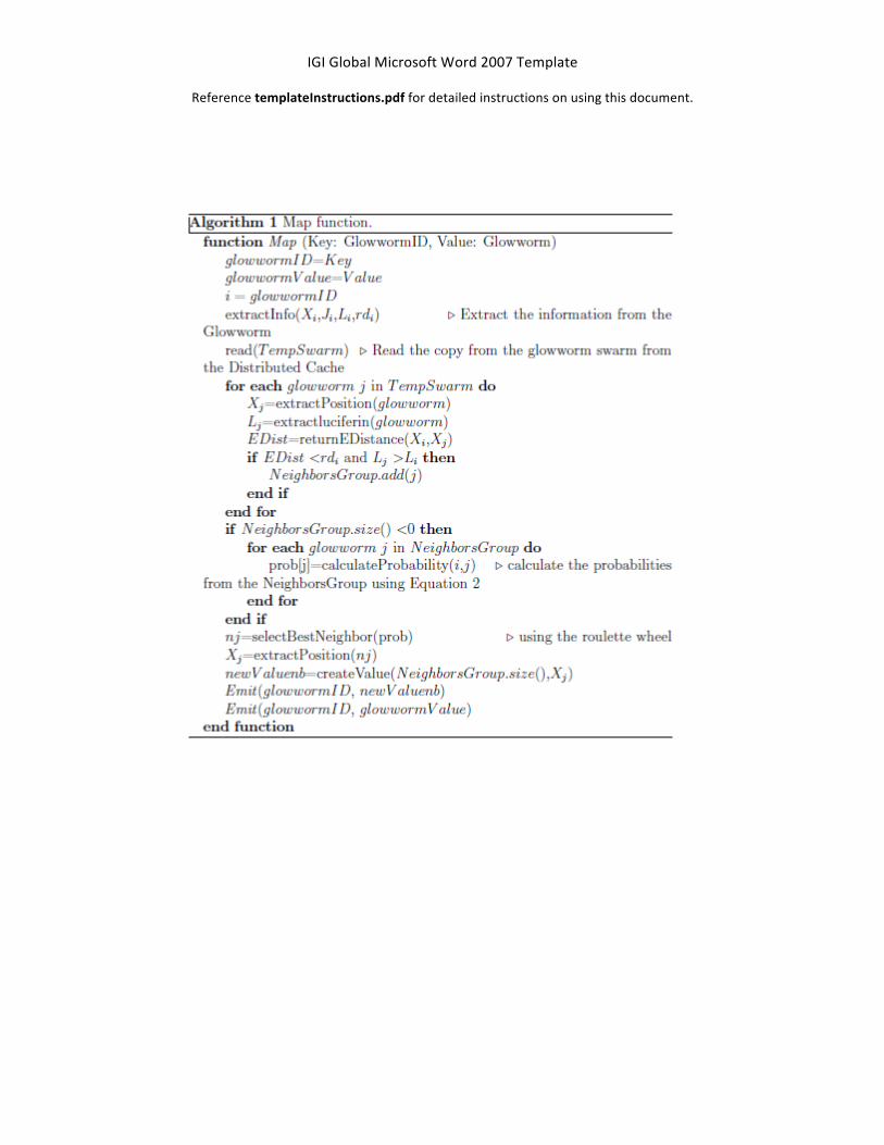
After that, the neighbor group finding process is started when the Map function receives <Key, Value> from the MapReduce job, where Key is the glowworm ID i and Value is the glowworm information. However, the Map function processes the Value by breaking it into the main glowworm components (Xi, J(Xi), Li, and rdi), which are used inside the Map function. Then, a local iterative search is performed on TempSwarm to locate the neighbor group using Equation (2). After that, the neighbor probability values are calculated based on Equation (3) to find the best neighbor using the roulette wheel selection method. At the end of the Map operation, the Map function emits the glowworm ID i with its Value and glowworm ID i with the selected neighbor position vector (Xj) to the Reduce function. The Map function works as shown in Algorithm 1 outlining the pseudo code of the Map operation.

As an intermediate step in the MapReduce job, the emitted intermediate output from the mapper function is partitioned using the default partitioner by assigning the glowworms to the reducers based on their IDs using the modulus hash function.

The Reduce function in the MapReduce job is responsible for updating the luciferin level Li, which is considered the most expensive step in the glowworm optimization, since in this stage the objective function is evaluated for the new glowworm position. The luciferin level updating process is started when the Reduce function receives < Key, ListofValues> from the Map function where Key is the glowworm ID and ListofValues contains the glowworm value itself and its best neighbor position (Xj). The reduce function extracts the neighbor position vector (Xj) and glowworm information (Xi, J(Xi), Li, and rdi). Then, the updating of the glowworm position vector is done using Equation (4). After that, the objective function is evaluated using the new glowworm position vector, and then the luciferin level is updated using Equation (1). Also, rdi is updated using Equation (5). At the end, the Reduce function emits the glowworm ID i with the newly updated glowworm information. The pseudo-code of the Reduce function is shown in Algorithm 2.

At the end of the MapReduce job, the new glowworm swarm replaces the previous swarm in the distributed file system, which is used by the next MapReduce job.



Experiments and Results In this section, we describe the optimization quality and discuss the running time of the

measurements for our proposed algorithm. We focus on scalability in terms of speedup and also on the optimization quality.

Environment We ran the MR-GSO experiments on the Longhorn Hadoop cluster hosted by the Texas

Advanced Computing Center (TACC1), which is one of the common Hadoop clusters that is used by researchers. The Longhorn Hadoop cluster contains 384 compute cores and 2.304 TB of aggregated memory capacity. The Longhorn Hadoop cluster has 48 nodes containing 48GB of RAM, 8 Intel Nehalem cores (2.5GHz each). For our experiments, we used Hadoop version 0.20 (new API) for the MapReduce framework, and Java runtime 1.6 to implement the MR-GSO algorithm.

Benchmark Functions To evaluate our MR-GSO algorithm, we used three multimodal benchmark functions. The

benchmark functions are the following (Engelbrecht et al., 2012, Qu et al., 2014):

• F1: The Equal-peaks-B function is a highly multimodal function in the m-dimensional search space. All local maxima of the Equal-peaks-A function have equal function values. The function search space ( !

!≤ 𝑋i≤

!! ) is used, where 𝑋i is the m-dimensional vector and i = 1,...,m. The

Equal-peaks-B function has 2m peaks like the Rastrigin function. The function has the following definition:

𝐹! 𝑋! = [𝑠𝑖𝑛!(!!!! 𝑋!)] (6)

• F2: The Rastrigin function is a highly multimodal function with the locations of the minima and maxima regularly distributed. This function presents a fairly difficult problem due to its large search space and its large number of local minima and maxima. We restricted the function to the hypercube ( −1 ≤ 𝑋i≤ 1 ); i = 1 ... m. The function has 2m peaks such as for m=2 dimensions, the function has 4 peaks within the given range. The function has the following definition:

𝐹! 𝑋! = 10𝑚 + [𝑋!! − 10cos (2π!!!! 𝑋!)] (7)

• F3: The Composition function is a very difficult multimodal function, which is constructed based on eight basic functions in the m-dimensional search space and contains different functions’ properties. The functions that are used to form this benchmark are Rastrigin, EF8F2, Weierstrass, and Griewank. Two versions from each basic function are used to construct the composition function, the original and rotated versions. We restricted the function to the hypercube (−5 ≤𝑋i≤ 5 ); i = 1 ... m. The function has 8 peaks within the given range. For more details regarding this function, refer to (Engelbrecht et al., 2012).

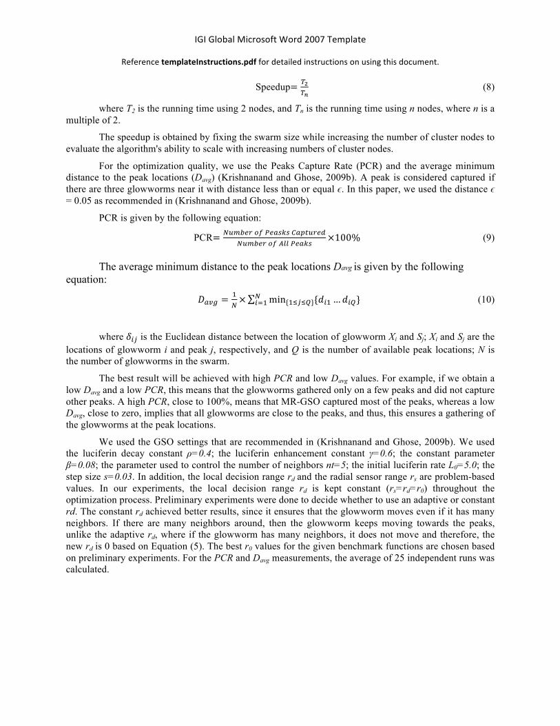
Evaluation Measures In our experiments, we used the parallel Speedup (Grama, 2003) measure to evaluate the

performance of our MR-GSO algorithm, which is calculated using the following equation: 1 https://portal.longhorn.tacc.utexas.edu/



Speedup= !!!!

(8)

where T2 is the running time using 2 nodes, and Tn is the running time using n nodes, where n is a multiple of 2.

The speedup is obtained by fixing the swarm size while increasing the number of cluster nodes to evaluate the algorithm's ability to scale with increasing numbers of cluster nodes.

For the optimization quality, we use the Peaks Capture Rate (PCR) and the average minimum distance to the peak locations (Davg) (Krishnanand and Ghose, 2009b). A peak is considered captured if there are three glowworms near it with distance less than or equal ϵ. In this paper, we used the distance ϵ = 0.05 as recommended in (Krishnanand and Ghose, 2009b).

PCR is given by the following equation:

PCR= !"#$%& !" !"#$%$ !"#$%&'(!"#$%& !" !"" !"#$%

×100% (9)

The average minimum distance to the peak locations Davg is given by the following

equation:

𝐷!"# =!!× min{!!!!!}{𝑑!!… 𝑑!"}!

!!! (10)

where 𝛿!" is the Euclidean distance between the location of glowworm Xi and Sj; Xi and Sj are the locations of glowworm i and peak j, respectively, and Q is the number of available peak locations; N is the number of glowworms in the swarm.

The best result will be achieved with high PCR and low Davg values. For example, if we obtain a low Davg and a low PCR, this means that the glowworms gathered only on a few peaks and did not capture other peaks. A high PCR, close to 100%, means that MR-GSO captured most of the peaks, whereas a low Davg, close to zero, implies that all glowworms are close to the peaks, and thus, this ensures a gathering of the glowworms at the peak locations.

We used the GSO settings that are recommended in (Krishnanand and Ghose, 2009b). We used the luciferin decay constant ρ=0.4; the luciferin enhancement constant γ=0.6; the constant parameter β=0.08; the parameter used to control the number of neighbors nt=5; the initial luciferin rate L0=5.0; the step size s=0.03. In addition, the local decision range rd and the radial sensor range rs are problem-based values. In our experiments, the local decision range rd is kept constant (rs=rd=r0) throughout the optimization process. Preliminary experiments were done to decide whether to use an adaptive or constant rd. The constant rd achieved better results, since it ensures that the glowworm moves even if it has many neighbors. If there are many neighbors around, then the glowworm keeps moving towards the peaks, unlike the adaptive rd, where if the glowworm has many neighbors, it does not move and therefore, the new rd is 0 based on Equation (5). The best r0 values for the given benchmark functions are chosen based on preliminary experiments. For the PCR and Davg measurements, the average of 25 independent runs was calculated.



Results To evaluate the MR-GSO algorithm, the experiments are done measuring PCR, Davg, running

time, and speedup for the mentioned benchmarks. In addition, the MapReduce overhead is also investigated. We will investigate the measures applied to all three benchmark functions. Figures 2 to 8 show the results for benchmark function F1, Figures 9-15 show the results for benchmark function F2, and Figures 16 to 19 show the results for benchmark function F3.

Figure 2 shows the optimization quality results for the F1 function with 2 dimensions. The PCR and Davg for every iteration using different numbers of swarm sizes (starting from 10,000 to 60,000) are presented. As can be noted from Figure 2(a), the PCR is improving for increasing swarm sizes. In addition, the number of iterations needed to capture all peaks is reduced, such as, the PCR converges to 100% with a swarm size of 10,000 at iteration 2, while with a swarm size of 60,000 the PCR converges at iteration 1. Also, Figure 2(b) shows that the average minimum distance is improved (reduced) when the swarm size is increased maintaining low values for all swarm sizes.

Figure 2: Optimization process for Equal-peaks-B function (F1) using 2 dimensions with 200 iterations, and r0=2.0. 2(a) Peaks capture rate. 2(b) Average minimum distance.

The optimization quality results for the F1 function with 3 dimensions are shown in Figure 3. Figure 3(a) clarifies the impact of the swarm size on the PCR. However, 19 iterations are needed to capture 100% of the peaks with a swarm size of 10,000, while with a swarm size of 60,000 the PCR converges to 100% at iteration 13. Also, Figure 3(b) shows that larger swarm sizes give better average minimum distance results maintaining low values for all swarm sizes.




Figure 4 shows the results for peaks capture rate and the average minimum distance for the F1 function with 4 dimensions. We note that 37 iterations capture 100% of the peaks with a swarm size of 10,000, while with a swarm size of 60,000 the PCR converges to 100% at iteration 27. Furthermore, the average minimum distance results maintain low values for all swarm sizes.




The PCR results for the F1 function with 5 dimensions are shown in Figure 5. MR-GSO needs 86 iterations to capture 100% of the peaks with 10,000 glowworms, but with 60,000, the PCR achieved 100% peaks capture rate at iteration 46. In addition, the average minimum distance results in Figure 5(b) show the best results with 60,000 glowworms.


The optimization quality results for the F1 function with 6, 7 and 8 dimensions are shown in Figures 6 to 8, respectively. All curves demonstrate the impact of the swarm size on the PCR, especially with increasing dimensions. In Figure 6(b), the peak capture rate results for 6 dimensions show that 200 iterations are needed to capture 93.75% of the peaks with a swarm size of 10,000, while 81 iterations with 60,000 glowworms are needed to capture 100%. Furthermore, using 7 dimensions, 200 iterations capture 22.66% of the peaks with a swarm size of 10,000, while with a swarm size of 60,000 the PCR converges to 100% at iteration 140 as shown in Figure 7. In Figure 8, the results with 8 dimensions are given. The results show that 200 iterations capture 2.73% of the peaks with a swarm size of 10,000, while with a swarm size of 60,000 the PCR converges to 64.84% at iteration 200.




Figure 9 to 15 show the optimization quality results for the F2 function with 2, 3, 4, 5, 6, 7 and 8 dimensions, respectively. Figure 9(a) shows that 1 iteration captures 100% of the peaks for 2 dimensions for all swarm sizes. The PCR results with 3 dimensions in Figure 10(a) show that 3 iterations capture 100% of the peaks with a swarm size of 10,000, while with a larger swarm size (60,000), the PCR converges to 100% at iteration 1. Furthermore, in Figure 11(a), 10 iterations capture 100% of the peaks with 10,000 glowworms, while PCR converges to 100% at iteration 6 with 60,000 glowworms. However, 23 iterations capture 100% of the peaks with 10,000 glowworms with 5 dimensions, while with a swarm size of 60,000 the PCR converges to 100% at iteration 14 with the same dimension. Lastly, the PCR results using 10,000 with 6,7, and 8 dimensions show that 200 iterations capture 98.44%, 16.41%, and 0.0% of the peaks, respectively. The PCR results using 60,000 with 6, and 7 dimensions show that 200 iterations capture 100.00%, while with 8 dimensions, PCR converges to 60.94%.

Figure 9: Optimization process for Rastrigin function (F2) using 2 dimensions with 200 iterations, and r0=0.5. 9(a) Peaks capture rate. 9(b) Average minimum distance.





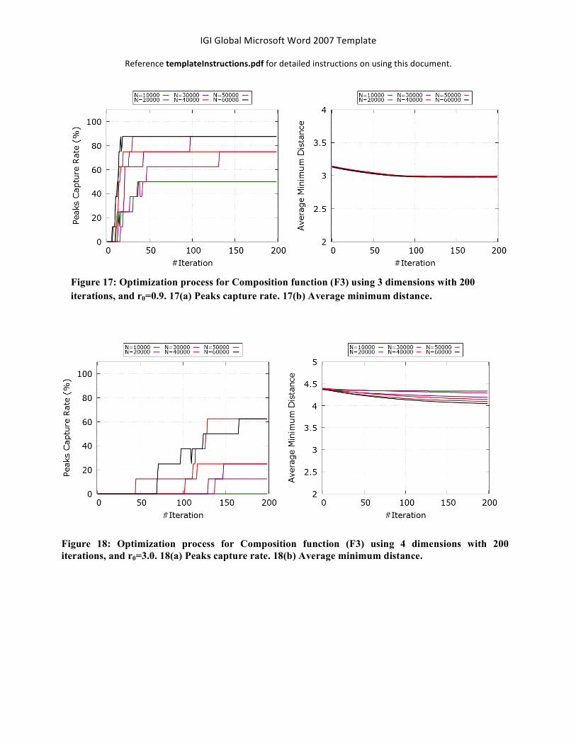
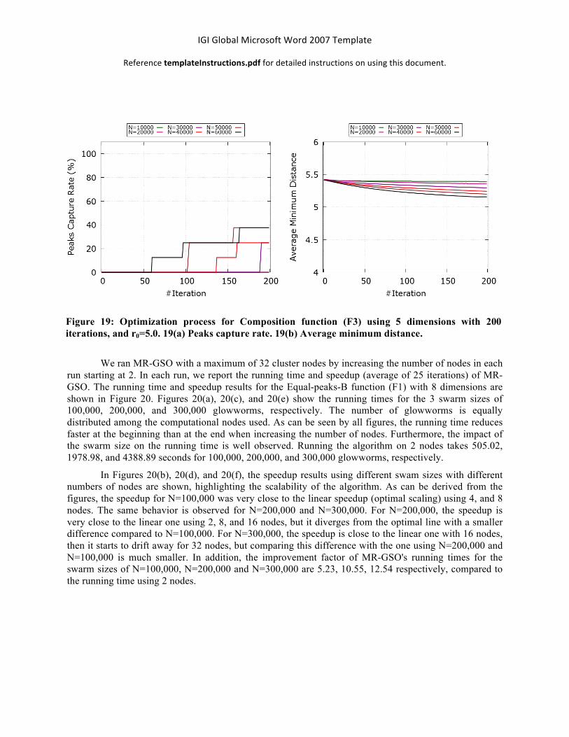
Figures 16 to 19 show the optimization quality results for the F3 function with 2, 3, 4, and 5 dimensions, respectively. Figure 16(a) shows that 20 iterations capture 100% of the peaks with a swarm size of 10,000, while with a larger swarm size (60,000) the PCR converges to 100% at iteration 1 already. The PCR results for 3 dimensions in Figure 17(a) show that 200 iterations capture 50% of the peaks with a swarm size of 10,000, while with a larger swarm size (60,000) the PCR converges to 87.5% at iteration 200. Lastly, the PCR results using 10,000 with 4 and 5 dimensions show that 200 iterations capture 0% of the peaks. On the other hand, the PCR results using 60,000 with 4 dimensions show that 200 iterations capture 62.5%, while with 5 dimensions PCR converges to 37.5%.

Figure 16: Optimization process for Composition function (F3) using 2 dimensions with 200 iterations, and r0=0.6. 16(a) Peaks capture rate. 16(b) Average minimum distance.



We ran MR-GSO with a maximum of 32 cluster nodes by increasing the number of nodes in each run starting at 2. In each run, we report the running time and speedup (average of 25 iterations) of MR-GSO. The running time and speedup results for the Equal-peaks-B function (F1) with 8 dimensions are shown in Figure 20. Figures 20(a), 20(c), and 20(e) show the running times for the 3 swarm sizes of 100,000, 200,000, and 300,000 glowworms, respectively. The number of glowworms is equally distributed among the computational nodes used. As can be seen by all figures, the running time reduces faster at the beginning than at the end when increasing the number of nodes. Furthermore, the impact of the swarm size on the running time is well observed. Running the algorithm on 2 nodes takes 505.02, 1978.98, and 4388.89 seconds for 100,000, 200,000, and 300,000 glowworms, respectively.

In Figures 20(b), 20(d), and 20(f), the speedup results using different swam sizes with different numbers of nodes are shown, highlighting the scalability of the algorithm. As can be derived from the figures, the speedup for N=100,000 was very close to the linear speedup (optimal scaling) using 4, and 8 nodes. The same behavior is observed for N=200,000 and N=300,000. For N=200,000, the speedup is very close to the linear one using 2, 8, and 16 nodes, but it diverges from the optimal line with a smaller difference compared to N=100,000. For N=300,000, the speedup is close to the linear one with 16 nodes, then it starts to drift away for 32 nodes, but comparing this difference with the one using N=200,000 and N=100,000 is much smaller. In addition, the improvement factor of MR-GSO's running times for the swarm sizes of N=100,000, N=200,000 and N=300,000 are 5.23, 10.55, 12.54 respectively, compared to the running time using 2 nodes.




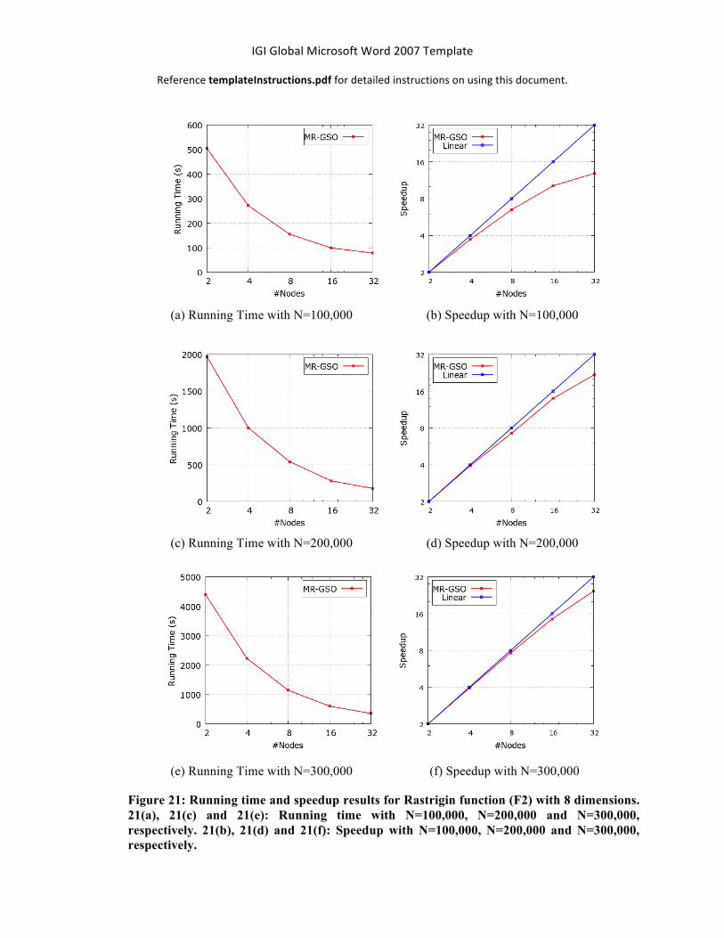
Figure 21 shows the running time and speedup results for the Rastrigin function (F2) with 8 dimensions. Figure 21(a) shows the running for the swarm size of 100,000. As more number of nodes are available (more hardware resources), the running time decreases. The same trend happens with 200,000, and 300,000 in the Figures 21(c), and 21(e), respectively. Running the algorithm on 2 nodes takes 505.39, 1967.18, and 4399.39 seconds for 100,000, 200,000, and 300,000 glowworms, respectively.

Figures 21(b), 21(d), and 21(f) show the algorithm speedup curve for the Rastrigin function (F2) and how an algorithm scales with respect to the linear speedup. The speedup values obtained with a swarm size of 100,000 with our proposed algorithm are almost linear up to 8 nodes such as the speedup is 3.7 for 4 nodes, 6.5 for 8 nodes, 10.2 for 16 nodes, and 12.9 for 32 nodes. For 200,000 glowworms, as shown in Figure 17(d), the speedup is close to the linear such as the speedup is 3.9 for 4 nodes, 7.3 for 8 nodes, 14.0 for 14 nodes, and 21.9 for 32, which are better speedup values compared to the swarm size of 100,000. For 300,000 glowworms as shown in Figure 21(f), the proposed algorithm achieves an almost linear speedup with 3.9 for 4 nodes, 7.7 for 8 nodes, 14.5 for 14 nodes, and 24.5 for 32, which are better speedup results compared to the swarm sizes of 100,000, and 200,000.



(a) Running Time with N=100,000 (b) Speedup with N=100,000

(c) Running Time with N=200,000 (d) Speedup with N=200,000

(e) Running Time with N=300,000 (f) Speedup with N=300,000

Figure 20: Running time and speedup results for Equal-peaks-B function (F1) with 8 dimensions. 20(b), 20(d) and 20(f): Running time with N=100,000, N=200,000 and N=300,000, respectively. 20(a), 20(c) and 20(e): Speedup with N=100,000, N=200,000 and N=300,000, respectively.



(a) Running Time with N=100,000 (b) Speedup with N=100,000

(c) Running Time with N=200,000 (d) Speedup with N=200,000

(e) Running Time with N=300,000 (f) Speedup with N=300,000

Figure 21: Running time and speedup results for Rastrigin function (F2) with 8 dimensions. 21(a), 21(c) and 21(e): Running time with N=100,000, N=200,000 and N=300,000, respectively. 21(b), 21(d) and 21(f): Speedup with N=100,000, N=200,000 and N=300,000, respectively.



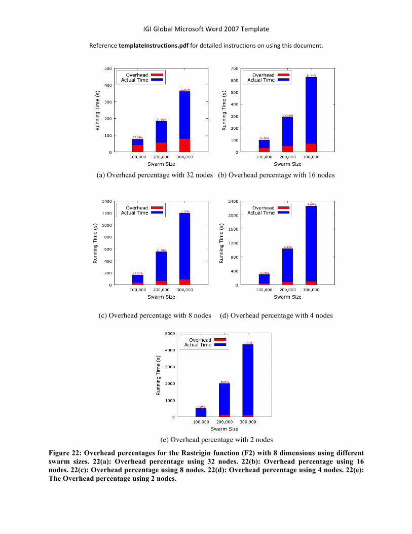
As we noted from the speedup figures, the system speedup diverges from the linear speedup when larger number of nodes are used. This happens because of the overhead of the Hadoop framework. The Hadoop framework introduces overhead due to the management of starting MapReduce jobs, starting mappers/reducers operations, serializing/deserializing intermediate outputs, sorting, and storing the outputs to the distributed file system. The impact of the MapReduce overhead percentages for the Rastrigin function (F2) with 8 dimensions and using different swarm sizes with different numbers of nodes are presented in Figure 22. The red portion in each column represents the overhead running time and blue portion represents the actual time for the function computations. In addition, the overhead percentage is given on top of each column. Figure 22(a) shows the overhead percentages using 32 nodes. We note that as the swarm size increases from 100,000 to 300,000, the overhead percentage reduces such as the overhead percentage for 100,000 is 55.04%, while the overhead percentage for 300,000 is 21.81% (less than half). The same trend is shown in Figures 22(b) to 22(e) using 10, 8, 4, and 2 nodes, respectively. Therefore, we can conclude that each additional node at some point contributes to increasing the overhead. Some of the Hadoop overhead is unavoidable and we should find the optimal number of nodes for each experiment, which balances the overhead and the algorithm performance. Furthermore, the overhead of the Hadoop framework can be avoided when using larger numbers of swarm sizes, and thus the speedup is closer to the optimal one.



Figure 22: Overhead percentages for the Rastrigin function (F2) with 8 dimensions using different swarm sizes. 22(a): Overhead percentage using 32 nodes. 22(b): Overhead percentage using 16 nodes. 22(c): Overhead percentage using 8 nodes. 22(d): Overhead percentage using 4 nodes. 22(e): The Overhead percentage using 2 nodes.

(a) Overhead percentage with 32 nodes (b) Overhead percentage with 16 nodes

(c) Overhead percentage with 8 nodes (d) Overhead percentage with 4 nodes

(e) Overhead percentage with 2 nodes



Conclusion This paper introduced a MapReduce-enabled Glowworm Swarm Optimization (MR-GSO)

algorithm for multimodal function optimization. GSO is particular useful for multimodal function optimization since it searches for multiple optima. MR-GSO parallelizes the GSO approach by implementing the map and reduce functions. The map function is responsible for the neighborhood calculations whereas the reduce function performs the luciferin level and the glowworm movement update. Two multimodal benchmark problems were evaluated for 2 to 8 dimensions in increments of 1. The first part of the evaluation captured the peak capture rate and the minimum distance for the different dimensions using different swarm sizes (10,000 and 60,000 in increments of 10,000). The measurements showed that with increasing dimensionality and difficulty of the benchmark problem larger swarm sizes are needed in order for the algorithm to find all peaks. The second part of the evaluation measured the running time and speedup of the MR-GSO algorithm. The number of computational nodes was scaled from 2 to 32 with double increments. The results showed that for both benchmark functions with the highest number of glowworms, the speedup was close to the linear speedup showing a good utilization of the parallel implementation of MR-GSO. In addition, the overhead of the Hadoop infrastructure was investigated showing an increase for larger numbers of glowworms used. In addition, the overhead more drastically increased for increasing number of computational nodes used. For example, using 32 computational nodes the overhead for 300,000 glowworms is 21.81%. Our future plan is to investigate the impact of the GSO settings on the optimization quality such as rs setting, and step size. Furthermore, we will apply the proposed algorithm on real world applications.

References Aljarah, I. & Ludwig, S. A. (2013a). A new clustering approach based on glowworm swarm optimization. In: IEEE Congress on Evolutionary Computation, IEEE, pp. 2642-2649.

Aljarah, I. &. Ludwig, S. A. (2013b). A mapreduce based glowworm swarm optimization approach for multimodal functions, in: Swarm Intelligence (SIS), IEEE Symposium on, pp. 22-31.

Barrera, J. & Coello, C. (2009). A review of particle swarm optimization methods used for multimodal optimization, in: C. Lim, L. Jain, S. Dehuri (Eds.), Innovations in Swarm Intelligence, volume 248 of Studies in Computational Intelligence, Springer Berlin Heidelberg, pp. 9-37.

Dean, J. & Ghemawat, S. (2008 ) Mapreduce: Simplified data processing on large clusters, ACM, pp. 107-113. vol 51.

DISCO. (2011). Disco mapreduce framework [Online]. Available: http://discoproject.org.

Engelbrecht, A. (2007). Computational Intelligence: An Introduction 2nd Edition, Wiley.

FACEBOOK. (2011). Hadoop - facebook engg, note. [Online]. Available: http://www.facebook.com/note.php?note id=16121578919.

Grama, A. & Gupta, A. & Karypis, G. & Kumar, V. (2003). Introduction to Parallel Computing, Addison-Wesley, USA.

Gunarathne, T. & Wu, T. & Qiu, J. & Fox, G. (2010). Cloud computing paradigms for pleasingly parallel biomedical applications, in: Proceedings of 19th ACM International Symposium on High Performance Distributed Computing, ACM, pp. 460-469.

Ismail, M. (2004). Parallel genetic algorithms (PGAs): master slave paradigm approach using MPI, in: E-Tech, pp. 83 - 87.



Jin, C. & Vecchiola, C. & Buyya, R. (2008). MRPGA: an extension of mapreduce for parallelizing genetic algorithms, in: Proceedings of the 2008 Fourth IEEE International Conference on eScience, ESCIENCE '08, IEEE Computer Society, Washington, DC, USA, pp. 214-221.

Kennedy, J. & Eberhart, R. (1995). Particle swarm optimization, in: IEEE International Conference on Neural Networks, volume 4, IEEE, pp. 1942-1948 vol.4.

Krishnanand. K. N., & Ghose, D. (2005). Detection of multiple source locations using a glowworm metaphor with applications to collective robotics, in: IEEE Swarm Intelligence Symposium, Pasadena, CA, USA, pp. 84 - 91.

Krishnanand, K. N., & Ghose, D. (2008). Glowworm swarm optimization algorithm for hazard sensing in ubiquitous environments using heterogeneous agent swarms, Soft Computing Applications in Industry, pp.165-187.

Krishnanand, K. N. & Ghose, D. (2009a). Glowworm swarm optimization: a new method for optimizing multi-modal functions, International Journal of Computational Intelligence Studies 1 (2009) 93-119.

Krishnanand, K. N. & Ghose, D. (2009b). Glowworm swarm optimization for simultaneous capture of multiple local optima of multimodal functions, Swarm Intelligence 3. 87-124.

Krishnan, S. & Baru, C. & Crosby, C. (2010). Evaluation of mapreduce for gridding LIDAR data, in: Proceedings of the CLOUDCOM '10, IEEE Computer Society, Washington, DC, USA, pp. 33-40.

Li, X., Engelbrecht, A., Epitropakis, M. G. (2013). Benchmark Functions for CEC'2013 Special Session and Competition on Niching Methods for Multimodal Function Optimization, Evolutionary Computation and Machine Learning Group, RMIT University, Melbourne, Australia.

MAPREDUCE. (2011). Apache software foundation, hadoop mapreduce [Online]. Available: http://hadoop.apache.org/mapreduce.

McNabb, A. & Monson, C. & Seppi, K. (2007). Parallel PSO using mapreduce, in: IEEE Congress on Evolutionary Computation, pp. 7-14.

Qu, B. Y., Liang, J. J., Suganthan P. N., and Chen Q. (2014). Problem definitions and evaluation criteria for the CEC 2015 competition on single objective multi-niche optimization, Computational Intelligence Laboratory, Zhengzhou University, Zhengzhou, China, Tech. Rep.

Stuetzle T. (2009). Ant colony optimization, in: Evolutionary Multi-Criterion Optimization, volume 5467 of Lecture Notes in Computer Science, Springer Berlin Heidelberg, 2009, pp. 2-2.

Snir, M. & Otto, S. & Huss-Lederman, S. & Walker, D. & Dongarra, J. (1995). MPI: The Complete Reference, MIT Press Cambridge, MA, USA. Tan, Q. & He, Q. & Shi, Z. (2012). Parallel Max-Min Ant System Using MapReduce. in: Proceedings of the ICSI Conference. pp. 182-189.

Venter, G. & Sobieszczanski-Sobieski, J. (2005). A parallel particle swarm optimization algorithm accelerated by asynchronous evaluations, Journal of Aerospace Computing, Information, and Communication.

Wong, L. P., & Low, M., & Chong, C. S. (2008). A bee colony optimization algorithm for traveling salesman problem, in: Proceedings of the 2008 Second Asia International Conference on Modelling & Simulation (AMS), AMS '08, IEEE Computer Society, Washington, DC, USA, pp. 818-823.

Wu, B. & Wu, G. & Yang, M. (2012). A mapreduce based ant colony optimization approach to combinatorial optimization problems, in: Natural Computation (ICNC), 2012 Eighth International Conference on, pp. 728 - 732.

YAHOO. (2011). Yahoo inc. hadoop at yahoo!! [Online]. Available: http://developer.yahoo.com/hadoop.



Zhou, C. (2010). Fast parallelization of differential evolution algorithm using mapreduce, in: Proceedings of the 12th Annual Conference on Genetic and Evolutionary Computation, GECCO'10, ACM, New York, NY, USA, pp. 1113-1114.

A Scalable MapReduce-enabled Glowworm Swarm …cs.ndsu.edu/~siludwig/Publish/papers/IJSIR2016.pdfA...

Documents

Transcript of A Scalable MapReduce-enabled Glowworm Swarm …cs.ndsu.edu/~siludwig/Publish/papers/IJSIR2016.pdfA...