A Safety Margin Model for Revenue Management in a Make-to ...
40
1 A Safety Margin Model for Revenue Management in a Make-to-Stock Production System Working paper 1. Introduction Although revenue management (RM) originates from service industries, its ideas are also relevant for manufacturing environment. In this paper, we consider RM approaches for demand fulfillment in a make-to-stock (MTS) production system with known exogenous replenishments and stochastic demand from multiple customer classes. We propose a safety margin model which borrows the “safety stock” idea from inventory management to account for demand uncertainty and sets up booking limits for each customer class. In a make-to-stock system, production is forecast-driven and cannot be easily adjusted to short-term demand fluctuation. Therefore, when demand is higher than supply, it may not be possible to satisfy all incoming customer orders. The manufacturer then has to decide how to allocate the limited supply, i.e., the finished goods inventory, to his customers, since different customers may show different profitability or hold different strategic importance. This situation is similar to the traditional airline revenue management problem, where a fixed number of seats are sold to multiple fare classes. Thus, demand fulfillment in MTS system can also benefit from revenue management ideas. The only difference is that, in the MTS system, the scarce resource to allocate is the finished goods inventory rather than seats. Unlike flight seats, inventory is storable and can be replenished at certain times. Therefore, inventory holding cost and backlogging cost might be incurred, which makes profit maximization a more appropriate criterion than pure revenue maximization.
Transcript of A Safety Margin Model for Revenue Management in a Make-to ...
1
A Safety Margin Model for Revenue Management in a Make-to-Stock
Production System
Working paper
1. Introduction
Although revenue management (RM) originates from service industries, its ideas are also
relevant for manufacturing environment. In this paper, we consider RM approaches for
demand fulfillment in a make-to-stock (MTS) production system with known exogenous
replenishments and stochastic demand from multiple customer classes. We propose a
safety margin model which borrows the “safety stock” idea from inventory management
to account for demand uncertainty and sets up booking limits for each customer class.
In a make-to-stock system, production is forecast-driven and cannot be easily adjusted
to short-term demand fluctuation. Therefore, when demand is higher than supply, it
may not be possible to satisfy all incoming customer orders. The manufacturer then has
to decide how to allocate the limited supply, i.e., the finished goods inventory, to his
customers, since different customers may show different profitability or hold different
strategic importance. This situation is similar to the traditional airline revenue
management problem, where a fixed number of seats are sold to multiple fare classes.
Thus, demand fulfillment in MTS system can also benefit from revenue management
ideas. The only difference is that, in the MTS system, the scarce resource to allocate is
the finished goods inventory rather than seats. Unlike flight seats, inventory is storable
and can be replenished at certain times. Therefore, inventory holding cost and
backlogging cost might be incurred, which makes profit maximization a more
appropriate criterion than pure revenue maximization.

2
In nowadays advanced planning system (APS), the available finished goods inventory
is represented by the so-called available-to-promise (ATP) quantities which are derived
from the mid-term master planning. For demand fulfillment, APS uses a two-level
planning process to answer real-time customer requests. In the first allocation planning
level, customers are segmented based on their profitability and/or strategic importance
and APS then allocates ATP quantities to different delivery periods and customer
segments according to certain predetermined allocation rules. In the second order
promising level, the allocated ATP (aATP) is consumed by the incoming orders based on
simple consumption rules such as first-come-first-served. The key connection between
the two planning levels is that, for each incoming order, if aATP is available for the
corresponding class, ATP can be consumed and the order is quoted accordingly.
Otherwise, the order promising process searches for other options to satisfy the order,
e.g., by consuming aATP quantities from lower classes if nesting is applied (Kilger and
Meyr 2008).
Obviously, the quality of the adopted allocation rule has a great impact on the
performance of demand fulfillment. For example, when supply is scarce, if two customer
segments with the same expected demand show very different profitability, it is
beneficial to allocate more supply to the more profitable segment than giving both
segments the same share. In the current APS practice, the ATP quantities are normally
allocated according to the priority ranks of the customers, the committed forecast, or
the predetermined split factors, all of which are merely simple heuristic rules and none
of them is profit maximizing.

3
In order to achieve system optimization, researchers have developed different
allocation planning approaches. One stream uses deterministic linear programming (DLP)
model to maximize the expected profit (Meyr, 2009). The other stream takes a full
stochastic perspective and models the problem as a dynamic program (Quante et al.
2009). Both of these approaches have limitations: The DLP model considers only
expected demand and neglects demand uncertainty, therefore not all information
included in the demand distribution is taken into account, which makes the solution
usually suboptimal. The stochastic dynamic program, however, is computationally
expensive and therefore hardly scalable.
As an alternative, this paper aims for incorporating the impact of demand
uncertainty into the deterministic model. In order to do so, we develop a safety-margin
model which has similar philosophy as the safety stock calculation. We consider the
same problem setting as Quante et al. (2009) and Meyr (2009): A make-to-stock
manufacturer is facing stochastic demand from heterogeneous customers with different
unit revenues. Inventory replenishments are scheduled exogenously and deterministic.
The manufacturer decides for each order whether to satisfy it from stock, backorder it at
a penalty cost, or reject it, in anticipation of more profitable future orders. The objective
is to maximize the expected profit over a finite planning horizon, taking into account
sales revenues, inventory holding costs, and backorder penalties.
We follow the two-level planning process of APS. In the allocation planning level, we
allocate the ATP quantities not only according to the expected demand, as Meyr (2009)
does, but also borrowing the “safety stock” idea from inventory management to
calculate “safety margins” for higher customer classes and set up corresponding booking
4
limits for the lower classes . By doing so, we successfully take demand uncertainty into
account.
For the order promising level, we quote the orders according to the predetermined
booking limits. In a series of numerical simulation, we compare the performance of our
safety margin model with other common fulfillment policies.
In summary, we make the following contributions to the field:
We present a new demand fulfillment model which takes customer demand
uncertainty into consideration.
By analogizing safety margins to safety stocks, we provide insight to the
relationship between the traditional inventory/supply chain management world
and the relatively new and emerging RM world.
We compare the relative performance of our safety-margin model and other
fulfillment policies numerically and show that the safety-margin model improves
the performance of the DLP model with even lower computational expense.
The paper is organized as follows. In § 2, we review the current literature and
further motivate our research. In § 3, we explain the problem setting and the basic
model formulation. The core of the paper is § 4, which derives the safety-margin model.
§ 5 provides a numerical study which compares the relative performance of common
current fulfillment policies in MTS environment. We conclude with §6 and discuss future
research potentials.

5
2. Literature review
In general, manufacturing systems can be divided into make-to-order (MTO) system,
assemble-to-order (ATO) system and make-to-stock (MTS) system. In literature, most
researches regarding RM in manufacturing focus on the MTO system. This is due to the
direct analogy between the perishable production capacity in MTO and the perishable
flight seats in the traditional airline RM, which makes most of the airline RM approaches
directly applicable in this environment. Van Slyke and Young (2000), Defregger and Kuhn
(2004, 2007), Rehkopf and Spengler (2005), Barut and Sridharan (2005), and Spengler et
al. (2007) propose RM approaches for the order acceptance problem in MTO
environment. Harris and Pinder (1995) apply RM to an ATO environment. Literature on
RM in MTS environment is very limited and we will focus on them in what follows.
Revenue management and manufacturing have significant methodological
differences. While revenue management is normally based on stochastic optimization
and uses probability distributions to assess opportunity costs, manufacturing companies
rely on APS which takes deterministic mathematical programming as the major tool for
different planning tasks (Quante et al. 2009). Due to this methodological divide between
revenue management and manufacturing, in literature there are two main streams of
researches for applying revenue management to demand fulfillment in MTS
manufacturing. The first stream holds the traditional APS perspective and seeks to
incorporate revenue management ideas into the deterministic optimization. The second
stream takes a full stochastic view and models the problem as dynamic program. In what
follows, we briefly review literature from both research streams.
6
For the deterministic stream, Kilger and Meyr (2008) set up a two-step framework, in
which demand fulfillment is accomplished through ATP allocation and ATP consumption.
Ball et al. (2004) propose a similar push-pull framework for ATP models: Push-based ATP
models pre-allocate available resources to different customer classes and pull-based ATP
models promise the allocated resources in direct response to incoming orders.
Following this framework, we first consider the allocation models.
Ball et al. (2004) develop a deterministic optimization-based model that allocates
production capacity and raw materials to demand classes in order to maximize profit.
They claim that the model is designed for an MTS environment, but actually it is more
appropriate for an ATO environment as both capacity and materials are taken into
account.
With the same problem setting as ours, Meyr (2009) proposes a deterministic linear
programming model for the ATP allocation. The DLP model maximizes the overall profit
and its optimal solution is used as partitioned quantity reserved for each customer class
and each arrival period, based on which different consumption rules are used for order
promising. A numerical study shows that, compared to the rule-based allocation
methods, this model can significantly improve the performance of an APS if demand
forecasting is reliable. This DLP model is computationally efficient and can therefore
easily be adapted to the advanced planning system. However, the major drawback is
that it utilizes only expected demand information but ignores demand uncertainty. In
order to overcome this drawback, our safety-margin approach extends the DLP model by
adding safety margins to expected demand to account for demand uncertainty.

7
Quante (2008) incorporates demand uncertainty into the DLP model in another way.
He adapts the randomized linear programming (RLP) idea from Talluri and van Ryzin
(1999) to the MTS setting. The idea is to repetitively solve the DLP, not with the
expected demand, but with a realization of the random demand with known distribution.
The optimal allocation quantity is estimated by a weighted-average of the results over
all repetitions. The RLP approach is appealing as it is only slightly more complicated than
the DLP method but incorporates distributional information on demand. Besides, it also
has the flexibility to model various possible demand distributions. However, according to
the numerical study from Quante (2008), the RLP model does not show promising
results and is often dominated by the DLP model.
After allocation planning, aATP quantities could be consumed in real-time mode or
batch mode. Kilger and Meyr (2008) propose to use search rules for real-time order
promising and suggest searching available aATP quantities along three dimensions:
customer class, time and product. In order to improve the rule-based consumption
methods which represent the current practice, Meyr (2009) formulates the real-time
order promising problem as a linear programing (LP) model with the objective to
maximize overall profits. In order to make it easy for practical implementation, he
proposes several consumption rules to mimic the LP search process. For batch mode
order promising, Fleischmann and Meyr (2003), Pibernik (2005, 2006) and Jung (2010)
propose optimization based models.
For the stochastic stream, Quante et al. (2009) model the demand fulfillment
process in MTS production as a network revenue management (NRM) problem and
formulate a stochastic dynamic program. Unlike the traditional airline network revenue
8
management problem, in the MTS setting, since products are identical, theoretically any
of the available supplies can be used to satisfy any incoming order. Therefore, one has to
decide not only whether or not to satisfy an order but also which supply and how many
of each supply to use, as each supply alternative generates a different profit. It turns out
that the optimal policy of the DP is the famous booking-limit policy which is easy to
implement. Quante et al. (2009) also show that it outperforms current common
fulfillment policies, such as first-come-first-served (FCFS) and the deterministic
optimization model from Meyr (2009). However, because of the “curse of
dimensionality”, it is computationally expensive and therefore not really applicable for
real-size problem. This paper considers the same problem setting as Quante et al. (2009)
and compares its performance with the proposed safety-margin model in the numerical
study.
In order to deal with the computational intractability, Bertsimas and Popescu (2003)
proposed a generic Approximate Dynamic Programming (ADP) algorithm, the basic idea
of which is to approximate the value function of the DP by a simpler algorithm, such as
linear programming (Talluri and van Ryzin 1999, Spengler et al. 2007, Erdelyi and
Topaloglu 2010), affine functional approximation (Adelman, 2007) and Lagrangian
relaxation approximation (Topaloglu 2009, Kunnumkal and Topaloglu 2010). Most of
these researches are within the traditional airline revenue management context and we
are not aware of any ADP study for the MTS environment.
In addition to the above mentioned two main streams, there is a paper from Pibernik
and Yadav (2009) that is closely linked to our setting: They also consider an MTS system
with stochastic demand. However, rather than pursuing the main target of revenue
9
management: profit maximization, the authors still use the traditional service level
maximization as the objective. Besides this main distinction, other differences include
that the authors limit their analysis to two classes and do not allow backlogging.

10
3. The Demand Fulfillment Model
We consider the same demand fulfillment problem and therefore share the same
problem setting with Meyr (2009) and Quante et al. (2009): We consider a MTS
manufacturing system with exogenously determined replenishments and stochastic
demand from heterogeneous customers. In order to maximize the expected profit, the
manufacturer has to decide for each arriving order whether to satisfy it from stock,
backorder it at a penalty cost, or reject it, in anticipation of more profitable future
orders. The manufacturer needs to take into account not only sales revenues, but also
inventory holding costs and backorder penalties.
Following the two-level framework from Kilger and Meyr (2008), we build up a
demand fulfillment model which comprises an allocation planning level and an order
promising level. In what follows, we summarize the modeling issues and notations for
the demand fulfillment model.
We have a finite planning horizon of T, which is subdivided into discrete time periods
. Customers are differentiated into different segments, , with
corresponding unit revenues of . Orders from different segments
arrive in arbitrary order and ask for a random quantity of the products. We assume that
the order due dates equal to the arrival date. This assumption is legitimate for the MTS
environment as customers normally expect immediate delivery. We use to denote
the total random demand from segment with arrival date . can follow any
possible distribution, e.g., Poisson, Normal or Negative Binomial.

11
At the beginning of the planning horizon, allocation planning is conducted once for
the whole planning horizon, with the following information on hand.
Available inventory that arrives in period which is denoted by ;
Demand forecast: The mean and standard deviation of is known.
After the allocation planning, incoming orders are processed in real time based on
the allocation result. Delaying an order causes backorder cost of per unit per period
and the unit holding cost is per period.
Table 1 Notation
Indices:
Periods of planning horizon
Demand due date
Customer segments
Data:
Unit revenue from customer segment
Unit backorder cost per period
Unit holding cost per period
Available ATP supply that arrives at the beginning of period
Random variables:
Total demand from segment with arrival date , follows a certain
distribution with known mean and standard deviation
Table 1 summarizes the above notations. The profit of one unit ATP from period
which is used for customer segment with arrival date can be calculated as follows
(1)
where is defined as 1 if and 0 otherwise (Quante et al., 2009).

12
Quante et al. (2009) model the above demand fulfillment problem as a stochastic
dynamic program and find out that the optimal policy is a generalized booking-limit policy
which sets up booking limit for each segment and supply arrival. This model generates the
optimal ex-ante policy and is easy to execute. The main problem is that it is computationally
expensive and therefore hardly scalable.
Using the partitioned allocation of each to segment with arrival date as the
decision variable, Meyr (2009) modeled the allocation planning problem as a DLP followed
by a rule-based consumption process. The DLP model is efficient to solve, but as only the
expected demand is taken into account, the performance is not satisfying if demand
uncertainty is high. Quante et al. (2009) show in the numerical study that for low demand
variability, the DLP model is competitive to the SDP model, but when demand variability
increases, the performance of the DLP model deteriorates drastically.
In order to overcome the limitations of the above two models, in the next section we
propose a safety margin model which can efficiently calculate the booking limits and also
takes demand uncertainty into account by incorporating safety margins to more profitable
customers.
13
4. Safety Margins
The basic idea of safety margin is analogous to the safety stock in inventory
management, i.e. to reserve more stock than expected demand as "safety margin" for
more profitable customers. We first consider a simple single-period, two-class case in
which safety margins can be calculated by Littlewood’s rule. Then we generalize the
calculation to multi-period, multi-class case.
4.1 Single period, two-class case
We first consider the problem with , and assume that within this single
period, the lower class (Class 2) arrives before the higher class (Class 1). The problem
then becomes the famous Littlewood’s problem and can be solved directly using
Littlewood’s rule. We now illustrate how its solution can be interpreted in terms of
safety margins.
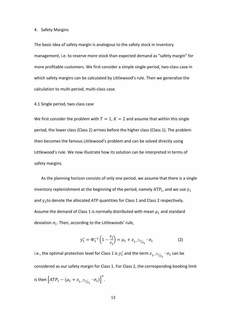
As the planning horizon consists of only one period, we assume that there is a single
inventory replenishment at the beginning of the period, namely , and we use
and to denote the allocated ATP quantities for Class 1 and Class 2 respectively.
Assume the demand of Class 1 is normally distributed with mean and standard
deviation . Then, according to the Littlewoods’ rule,
( )
⁄ (2)
i.e., the optimal protection level for Class 1 is and the term
⁄ can be
considered as our safety margin for Class 1. For Class 2, the corresponding booking limit
is then [ ⁄ ]
.

14
Similar to the safety stock idea, we add a safety margin for the Class 1 customers in
the allocation planning stage to better protect them.
Incorporating the safety margin of Class 1 into the DLP model from Meyr (2009),
which is discussed in the previous chapter, the allocation planning problem can then be
modeled as follows.
(3)
subject to
⁄ (4)
(5)
(6)
Constraint(4) modifies the DLP model by adding the safety margin ⁄ in
addition to the mean demand for Class 1. This simple LP forms a continuous knapsack
problem whose solution is equivalent to the Littlewood’s rule, i.e., by incorporating the
safety margin term, we make the DLP model equivalent to the Littlewood’s model which
is optimal for our single-period, two-class case. This idea can be further extended to the
multi-period, multi-class case.
4.2 Multi-period, multi-class case
Unlike the previous single period, two-class case, it is difficult to use the Littlewood’s
rule directly to calculate the safety margins for the ATP allocation problem in our MTS
setting due to the following three characteristics: (1) It involves multiple customer
classes instead of only two. In our MTS setting, we have multiple customer segments
and in addition, orders from the same segment with different arrival dates incur

15
different inventory holding or backlogging costs, and thus provide different profit.
Therefore, these orders cannot be treated as a single class. This cost impact is a major
difference between our MTS setting and the traditional airline RM, where orders from
the same customer segment always generate the same profit. (2) The “low-before-high”
assumption of Littlewood’s rule is violated. The MTS setting involves multiple planning
periods and within each period, orders from any customer segment may arrive.
Therefore, orders arrive earlier may generate higher profits than orders arrive later. (3)
It considers multiple replenishments, i.e., unlike the single resource case in Littlewood’s
model, we have multiple resources to allocate.
In order to deal with the first difficulty mentioned above, i.e., multiple customer
classes, we adopt the idea of the expected marginal seat revenue (EMSR) heuristic
which extends the Littlewood’s rule to multi-class case (Belobaba, 1989). We consider
each customer segment with a different arrival date as a different class. For a planning
horizon of periods with customer segments, we have in total customer
classes.
According to standard EMSR which also assumes low-revenue demand arrives before
high-revenue demand, the profit ranking of the classes should correspond to their
arrival date, i.e., the one with the lowest profit arrives earliest and the one with the
highest profit arrives latest. With this “low-before-high” assumption, EMSR ensures that
the future higher classes are protected against the current lower class. However,
assuming this “low-before-high” pattern is not reasonable in our MTS setting as we
know that the inherent time structure of our arriving process is not the case: Each of the
classes has its specified arrival date which does not follow the “low-before-high”

16
pattern. Therefore, the second difficulty still remains. In order to deal with it, as we
know the exact arrival period of each class, we first rank them in a descending order of
their arrival date. For classes with the same arrival period, we do not know their exact
arrival sequence and assume that the lower classes arrive before the higher ones, i.e.,
they are ranked in a descending order of their unit revenue . Then, the first class is the
one from Segment 1 that arrives in the last period and the last class is the one from
Segment that arrives in the first period. By doing so, we ensure that by using EMSR we
are indeed protecting the future classes against the current one. Furthermore, at each
stage of the EMSR heuristic, when calculating the protection level, we only consider the
future classes with higher profit than the current one. By doing so, we also achieve the
goal of the standard EMSR, i.e., to protect the future higher classes against the current
lower one.
To deal with the third difficulty, namely, the multiple resources, we consider two
variants. First, we simply consider the multiple ATP supplies separately, i.e., we calculate
the protection levels with respect to each ATP supply as if it is the only resource to
allocate, without considering the impact of other supplies. The problem with this
approach is that we are “double-counting” the demand of the higher classes when
calculating protection levels – this method assumes that the future demand can only be
fulfilled by a single ATP supply (the one under consideration) while actually, it has access
to all ATP supplies. One may expect that this “double-counting” problem makes the
safety margin model over-protect the higher classes. In order to deal with this problem,
we consider another variant, i.e., to implicitly allocate the demand to individual supply:
For each ATP supply, when determining the corresponding protection levels, we only
take the future demand that arrive before the next supply into account. On contrary to

17
the first case, the potential drawback of this approach is that we may not protect
enough for the higher classes as we consider only a fraction of the demand when
calculating the protection levels. We call the safety margin model with the first approach
Safety Margin Model_Version 1(SM_1) and with the second approach Safety Margin
Model_Version 2(SM_2).
4.2.1 Safety Margin Model_Version 1
Following the two-level planning procedure of APS, we first explain SM_1 in more detail
with the following steps.
Allocation Planning
1. Define classes
Rank the classes in a descending order of their due date. Classes with the
same due date are ranked in a descending order of their unit revenue . Use a new
index to denote customer classes and can be considered as the
customer segment/due date combination index. There is a one-to-one
correspondence between each and a combination of .
2. Calculate safety margins
For each ATP supply , do the following calculation:
a. At stage , let denote the set of future classes which have higher unit
profit than class if is used, i.e., { { }
}.
b. Define the aggregated demand of set by

18
∑
( 7)
c. Define the weighted-average profit of set by
∑ [ ]
∑ [ ]
(8)
d. Calculate the safety margins
According to the Littlewood’s rule, the protection level for set is
(
) (9)
where ∑ and stands for the safety margin for set .
If, the demand for each Class is normally distributed with mean and variance
, we have
(10)
where
∑
(11)
(
) (12)
3. Incorporate safety margins to the DLP model
Adding the safety margins into the DLP model, the resulting allocation planning
model is as follows
∑∑
(13)
subject to
∑
(14)

19
∑
(15)
(16)
Constraint (14) shows that this model indeed incorporates safety margins in
addition to expected demand for the higher classes.
We can use the solution of the above LP as the allocation result. Note that the above
LP can actually be decomposed into single-resource problems, i.e., we can have an
individual LP for each supply . This is because in the safety margin calculation (Step
2), we explicitly consider each supply separately and determine the set of future
higher classes ( ) with respect to the specific supply . Therefore, the obtained
safety margins in Constraint (14) are for each individual supply . Besides, in
the above LP, there is no constraint specifying the relation between different
supplies.
However, a more convenient way is to write down the corresponding booking limits
directly without solving the LP. We are able to do so because that Constraint (14)
already implies a booking limit for Class , namely
[ ]
(17)
Another advantage of using the booking limits directly is that, as we do not need to
know the exact allocation to each class and the protection level term in (17)
is independent of the real ATP consumption, in the later order processing stage, we
only need to update the current quantities before we process each incoming
order. It is not necessary to repeat the allocation planning steps all over again. If we
use the solution of the above LP as the allocation result, we need frequent re-solving
to adapt our allocation to the real consumption.

20
Order Processing
In the order promise stage, we process the incoming orders in real time. The following
procedure is used for processing an order from Class j ( ) with an order
quantity of d.
1. Update the current quantities for each supply .
2. Determine the corresponding booking limits using (17). Note that our way of
safety margin calculation sets nested booking limits for classes with the same arrival
period, i.e., within the same period, higher classes have always access to units
allocated to the lower classes.
3. Search for ATP supplies to fulfill the order successively, in the order of their arrival.
Let denote the amount of ATP quantities from supply t used to satisfy the given
order, we have the following steps:
Start with ;
Set ( ( ∑ ) )
Repeat for .
What needs to be noticed is that the safety margins and the protection levels from
(9) are independent of . Therefore, before each order processing, we only need to
update the current quantities to determine the current booking limits. It is not
necessary to repeat the allocation planning steps.
In the order processing, we start our search for available ATP quantities from the
earliest available ATP supply. This is because we know from Quante et al. (2009) that
under certain assumptions, the optimal policy for this MTS demand fulfillment situation
is also a booking-limits policy and the optimal solution is obtained through a line search,

21
starting with the earliest available supply. Here, we are mimicking the optimal behavior
in our order processing level.
4.2.2 Safety Margin Model_Version 2
For SM_2, its only difference compared to SM_1 is that when calculating the protection
level with respect to each ATP supply, it only considers future demand that arrive before
the next ATP supply. Therefore, it has the same procedure as SM_1 and we only need to
modify set (Step 2a of the allocation planning level) as follows.
For each ATP supply , assume the next non-zero ATP replenishment arrives at the
beginning of period { } At stage , { {
} } Since there is a one-to-one correspondence
between each class index and combination, here denotes the arrival date of
Class .
As mentioned above, before each order processing, it is not necessary for the safety
margin models to repeat the allocation planning steps due to the fact that they adopt
the booking-limit policy and the safety margins we calculate are independent of the real
consumption. But for the DLP model, in the allocation planning, it explicitly allocates the
available ATP quantities to different classes and therefore needs frequent re-planning to
adjust its allocation according to the real consumption. Otherwise, its performance
might be hurt. Because of the above mentioned difference, the safety margin model we
propose is computationally more efficient than the DLP model. We illustrate this further
in next chapter using run-time analysis.
22
5. Numerical Study
In order to evaluate the performance of different demand fulfillment models, Quante et
al. (2009) set up a numerical study framework, comparing their stochastic dynamic
programming model (SDP) to a first-come-first served strategy as well as the
deterministic linear programming model from Meyr (2009). Following the same
assumptions as Quante et al. (2009), we add both versions of safety margin models to
the numerical study framework.
Same as Quante et al. (2009), we consider a finite planning horizon here in order to
make the models comparable to the SDP model. However, the safety margin models we
propose, as well as the DLP model are also applicable in rolling-horizon planning.
Within the finite planning horizon, it is not necessary for the safety margin models or
the SDP model to do any re-planning, because both methods calculate the booking limits
upfront and the obtained booking limits are independent of the real ATP consumption.
The DLP model, on the other hand, allocates the current ATP quantities in the allocation
planning stage; therefore it is necessary to do re-planning frequently so that it has the
chance to adjust its allocation according to the real consumption.
In what follows we compare the performance of the safety margin models with the
following fulfillment strategies:
First-come-first served (FCFS): A comparison with this strategy shows us the
benefit of customer segmentation in the demand fulfillment process. To ensure
fairness, we limit this policy to fulfill customer orders only from stock to avoid
excessive backordering.
23
Deterministic linear programming (DLP) model from Meyr (2009): As explained in
the previous sections, this strategy allocates the ATP quantities using a DLP
model, followed by a rule-based consumption process: The search starts in each
incoming order’s own priority class. It first looks for aATP quantities that arrives
at the required due date. If the order is not fully satisfied, it searches further for
aATP quantities that arrive before the due date and then after the due date.
Finally, it repeats the search in lower classes. In the numerical study we
recalculate the DLP model after each order processing to ensure its performance.
A comparison with this strategy provides an indication of the benefit of
incorporating demand uncertainty in the fulfillment process.
Stochastic dynamic programming (SDP) model from Quante et al. (2009): This
strategy models the demand fulfillment process as a stochastic dynamic program,
whose optimal policy is also a booking-limits control. This strategy maximizes the
expected profit and therefore generates the optimal ex-ante policy.
Global optimum (GOP): This strategy optimally allocates ATP quantities to
demand ex-post and therefore provides the highest achievable profits. In the
numerical study we use it to normalize the results for comparison.
We follow the same assumptions as Quante et al. (2009) for the demand pattern:
Orders of a given customer segment follow a compound Poisson process and the order
processes of different segments are mutually independent. We discretize the planning
horizon in such a way that at most one order could arrive in a single period and the
probability of no order arrival is . This single-order-arrival assumption is made for the
SDP model as it is required by the Bellman equation formulation, but not necessary for

24
the safety margin model. For each given arrival, the order size follows a negative
binomial distribution (NBD). This choice allows us to analyze the effects of large demand
variations. In order to make the order size strictly positive, we model it as
, where is the mean and is the standard deviation. Modeling the
ordering process as a compound Poisson process makes twofold variability for the
customer demand, i.e., the customer demand variability depends on both the variability
of the order size as well as the arrival probabilities.
Based on the above assumptions, we define a numerical experiment with a test bed
containing a wide range of problem instances and use simulation to evaluate the
performance of the above mentioned models. In subsection 5.1 we define the test beds
and in subsection 5.2 we analyze the results of the numerical study.
5.1 Test bed
We design our test bed based on a full factorial design with five design factors and six
fixed parameters. We fix our planning horizon to 14 periods with two inventory
replenishments in period 1 and period 8. Replenishments quantity is fixed to 50 units
each time, i.e., . We consider 3 customer segments with different
revenues. Inventory holding cost is fixed to $1 per unit per period. We assume that the
mean demand of each incoming order is constant and equal to 12 units. We summarize
our choices for the design factors and fixed parameters in Table 2. This setup is similar to
Quante et al. (2009), but Quante et al. (2009) consider only the first three design factors
but assume equal order arrival probabilities and a fixed backlogging cost of $10 per unit
per period for all customer segments.

25
Table 2 Design factors and fixed parameters for the numerical study
Name Value
Fixed parameters
Planning horizon ( ) 14
Arrival periods of replenishments Period 1, Period 8
Replenishments quantity ( ) 50
Number of customer segments ( ) 3
Inventory holding cost ( ) 1
Mean demand per order ( ) 12
Design factors
Coefficient of variation of order size ( ) {
}
Customer heterogeneity ( ) { }
Supply shortage rate ( ) { }
Customer arrival ratio ( ) { }
Backlogging cost proportion ( ) { }
The total number of all possible combinations for these design factors is
, i.e. we have 324 scenarios. For each scenario, we generate 30 different demand
profiles and run the corresponding simulations for every policy. This gives us in total
instances for each policy in our numerical study. This scenario size
ensures that both of the type I and type II error of the factorial design is limited to 5%.
We now explain the design factors in detail. The first factor in the factorial design is
the coefficient of variation of order size ( ). We fix the mean of the order size to

26
, but the actual order size can vary from order to order and the variation is
represented by the coefficient of variation of the order size ⁄ , where is the
standard deviation of the order size. We choose the same range of as Quante et al.
(2009) to ensure a reasonable range of variability.
The second factor of the factorial design is customer heterogeneity, which is
represented by the revenue vector of the customer segments. The
revenue vector represents a low customer heterogeneity while
represents a high customer heterogeneity. These choices are also identical
to Quante et al. (2009).
The third factor of the factorial design is the supply shortage rate ( ), which reflects
the degree of supply scarcity. It is defined as follows:
∑
Since in our case the supply quantity and the mean demand of each order are both
fixed, the supply shortage rate ( ) depends solely on the no arrival probability . A
large corresponds to a low shortage rate while a small leads to a high shortage rate.
In our factorial design, we vary between 1% and 40% by varying from 0.4 to 0. We
choose these levels because since we only consider situations where supply is scarce, 1%
shortage rate is almost the lowest shortage rate we can use and 40% corresponds to a
no arrival probability of 0 and is therefore the highest shortage rate we can use. Quante
et al. (2009) use the same levels for the shortage situation, but also consider two more
levels for oversupply, i.e., being negative.
27
The fourth factor of the factorial design is customer arrival ratio ( ). This factor
reflects the fraction of demand from each customer segment. For instance, when no
arrival probability , a customer arrival ratio corresponds with an
arrival probability of for Segment 1, for Segment 2 and for Segment 3.
The fifth factor of the factorial design is the backlogging cost proportion ( ). Quante
et al. (2009) assume a fixed backlogging cost for all customer segments. We generalize
this assumption to allow different backlogging cost for different customer segments, as
customers from different segments pay different prices. In the numerical study, we
assume that the backlogging cost for different customer segment is proportional to the
corresponding revenue. When this proportion is small, e.g., , backlogging
penalty is low and when this proportion is large, e.g., , backlogging cost takes 20%
of the revenue, which makes the penalty high. Considering the holding cost , the
chosen levels of backlogging cost ratio ensure that the resulting service level is within a
reasonable range, e.g., if we fix the other parameters to their middle values (i.e.,
), our replenishment schedule
achieves an average cycle service level between 56% and 82% for all segments if we vary
from 0.05 to 0.2.
5.2 Results Analysis
Using the test bed, we obtain the simulated profits of all the 9720 instances for each
of the fulfillment strategies mentioned in the previous section. The average run-time for
one simulation instance is 1774.56 seconds for the SDP model, 26.45 seconds for the
DLP model, 3.63 seconds for the SM_1 model and 3.47 seconds for the SM_2 model,
using a standard PC with a 2.0GHz Intel Core 2 Duo CPU and 2.00GB memory. The run-

28
time data shows that the safety margin models are indeed much more efficient than the
SDP model and even faster than the DLP model.
By comparing the simulated profits of other strategies to the simulated profits of the
GOP model, we obtain the optimality gaps. We then calculate the average optimality
gap for the FCFS strategy, DLP model, SDP model, and both versions of the SM model
over (i) all 9720 test instances, and (ii) all subsets where one of the design factors is fixed
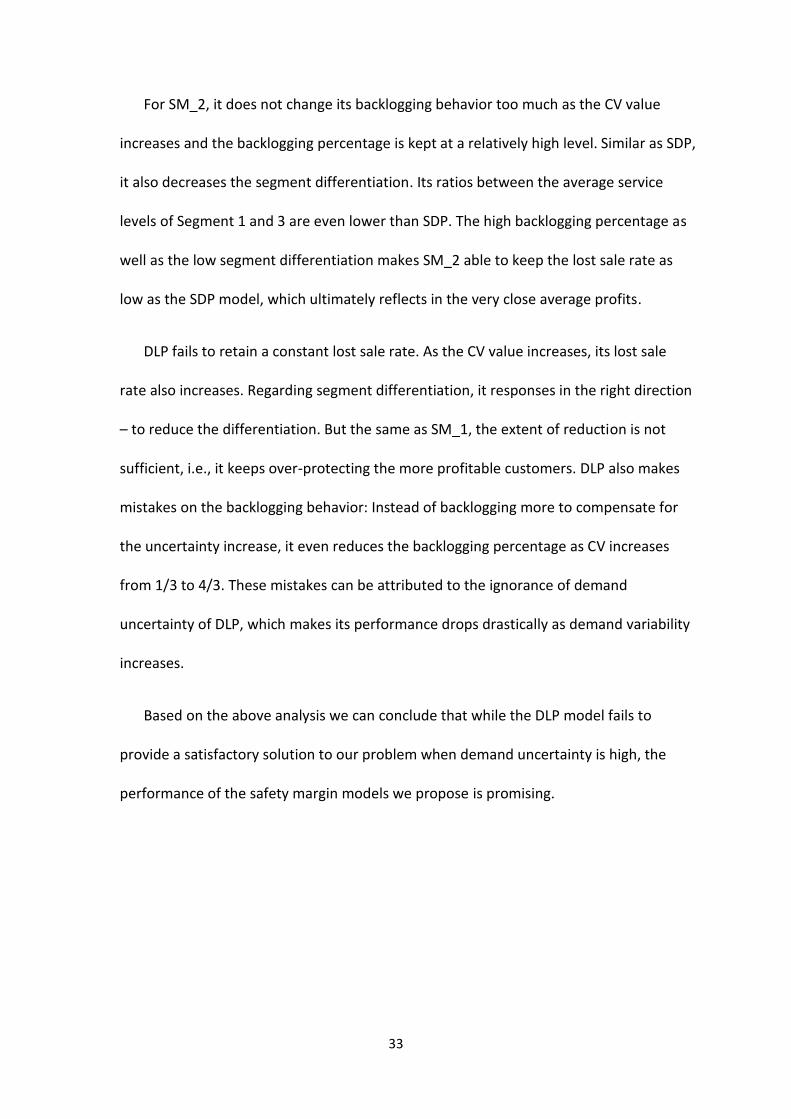
to one of its admissible values. The results are shown in Table 3. Beside the average
optimality gap (shown in bold), we also show the average backlog percentage (first value
in parenthesis), the average lost sales percentage (second value in parenthesis) and the
ratio between the average service levels of Segment 1 and Segment 3 (third value in
parenthesis) of each strategy. As complementary data, the second and third row of
Table 3 shows the average backlogging percentage and average lost sale percentage of
each customer segment over all instances for each fulfillment model.
From the first row in Table 3, we see that as expected, the SDP model performs best
with an average optimality gap of 3.96%, followed by SM_2 and SM_1 with an average
optimality gap of 4.57% and 5.45% respectively. On average, the FCFS strategy (with an
optimality gap of 7.55%) performs better than the DLP model (with an optimality gap of
8.84%).
Regarding the safety margin model, apparently both versions are considerably better
than the DLP/FCFS model and perform much closer to the SDP model. As the safety
margin models are developed to overcome the limitations of the DLP model and the SDP
model, in what follows we will focus on comparing the safety margin models to these
two models to disclose the difference.
29
By comparing the difference between the optimality gaps, we can see that SM_1
covers about 70% of the discrepancy between the DLP model and the optimal SDP
model, and SM_2 covers 87% of the discrepancy.
As the SDP model provides the optimal solution to our problem, we compare the
decisions (i.e., the backlogging, lost sale and service level behavior reflected in the
bracketed value of Table 3) made by the two safety margin models and the DLP model
to it to understand the profit differences.
Regarding lost sales, the SDP model has an average lost sale of 24.39%. Considering
different customer segments, it has the highest lost sale rate for Segment 3 and the
lowest rate for Segment 1. If we further consider its backlogging behavior we can see
that it backlogs much more for Segment 1 and 2 than for Segment 3. Based on this
observation we may conclude that compared to the other methods, the SDP model
achieves a relatively high service level for the more profitable customers by increasing
backlogging.
Compared to the SDP model, the DLP model has a higher average lost sale (28.11%).
However, for Segment 1, its lost sale rate is even lower than SDP, but it loses much more
customers from Segment 2 and 3. Regarding backlogging, the DLP model backlogs less in
average and does not show a clear differentiation between segments. The backlogging
rate for both Segment 1 and 2 are lower than SDP, i.e., the DLP model achieves a higher
service level for Segment 1 with even less backlogging, but at the cost of losing much
more customers from Segment 2 and 3. This provides clear evidence that the DLP model
tends to over-protect high profit customers. This “over-protection” problem of DLP has
also been identified by previous researches (De Boer, Freling, & Piersma, 2002).
30
The SM_1 model results in a lower lost sale rate (26.61%) than the DLP model. For
Segment 1 and 2, its performance is very close to the SDP model, but for Segment 3, it
has the highest lost sale rate among all methods. This means that our SM_1 model has
also the “over-protection” problem, presumably due to the “double-counting” effect we
have discussed in the previous chapter. Regarding backlogging behavior, SM_1 has a
higher backlogging percentage than DLP, especially for Segment 1 and 2. Based on the
behavior pattern of SDP we know that this backlogging behavior is actually favorable
and might be the reason that SM_1 has less lost sale compared to DLP, which ultimately
results in a higher average profit.
Considering our SM_2 model which is proposed to deal with the “double-counting”
effect, from Table 3, we can see that is has the lowest lost sale rate (24.33%), even lower
than the SDP model. This might be because that it loses more Segment 1 orders than the
other strategies but much fewer Segment 3 orders and therefore indeed releases the
“over-protection” problem. Considering the backlogging behavior, we can identify that it
has the same pattern as the SDP model – increasing backlogging for more profitable
customers to achieve better service level. From Table 3 we can see that SM_2 backlogs
even more than the SDP model and this might explain why the average profit of SM_2 is
still lower than SDP although it has the lowest lost sale rate.
The following part of Table 3 provides valuable information on the impact of
different design factors on the performance of each fulfillment model. The customer
arrival ratio ( ) and the backlogging cost proportion ( ) have little impact on the
performance of the models, as for different levels of these two design factors the
resulting optimality gaps of each fulfillment model are nearly the same. For the

31
coefficient of variation of order size ( ), customer heterogeneity ( ), and supply
shortage rate ( ), we find out that they have greater impact on the resulting optimality
gap of each model and we analyze the impact in what follows.
Coefficient of variation of order size ( )
From Table 3 and the following Figure 1, we can see the clear dependency between the
optimality gaps and the CV values.
Figure 1 Average optimality gap for different CV values
We observe the following: (1) In general, as the CV value increases, all strategies
show an increasing trend in their average optimality gaps. (2) For small CV values (i.e.,
low demand variability), the performance of DLP and the safety margin models are close
to each other. However, as the demand variability increases the performance of the DLP
model drops drastically. On the other hand, the performances of the two safety margin
32
models are always very close to the SDP and evidently better than the DLP model for
larger CV values. As the CV value increases, the gap between SM_2 and SDP is even
getting closer.
For the first observation, the potential explanation is that the increasing demand
variability leads to an increasing forecast error, which hurts the performance of every
strategy.
In order to explain the rest observations regarding the individual performance of
each model, we first summarize the response of SDP, as it provides the “right” response
to parameter changes. Then we compare the decisions made by the other strategies to
it.
As the CV value increases, SDP is able to keep the average lost sale rate almost
constant. The backlogging percentage increases and the ratio between the average
service levels of Segment 1 and 3 decreases. Based on these observations we may
conclude that, as demand uncertainty increases, SDP reduces the differentiation
between segments and backlogs more to retain the average service level.
Regarding backlogging, SM_1 responses the same as SDP - it increases the
backlogging percentage to cope with the increasing demand uncertainty. It also reduces
the differentiation between segments. However, the reduction extent is not sufficient,
as its ratios between the average service levels of Segment 1 and 3 are always higher
than that of the SDP model. The above reactions enable SM_1 to keep the lost sale rate
at an almost constant but higher level.
33
For SM_2, it does not change its backlogging behavior too much as the CV value
increases and the backlogging percentage is kept at a relatively high level. Similar as SDP,
it also decreases the segment differentiation. Its ratios between the average service
levels of Segment 1 and 3 are even lower than SDP. The high backlogging percentage as
well as the low segment differentiation makes SM_2 able to keep the lost sale rate as
low as the SDP model, which ultimately reflects in the very close average profits.
DLP fails to retain a constant lost sale rate. As the CV value increases, its lost sale
rate also increases. Regarding segment differentiation, it responses in the right direction
– to reduce the differentiation. But the same as SM_1, the extent of reduction is not
sufficient, i.e., it keeps over-protecting the more profitable customers. DLP also makes
mistakes on the backlogging behavior: Instead of backlogging more to compensate for
the uncertainty increase, it even reduces the backlogging percentage as CV increases
from 1/3 to 4/3. These mistakes can be attributed to the ignorance of demand
uncertainty of DLP, which makes its performance drops drastically as demand variability
increases.
Based on the above analysis we can conclude that while the DLP model fails to
provide a satisfactory solution to our problem when demand uncertainty is high, the
performance of the safety margin models we propose is promising.
34
Table 3 Simulation results
Test bed subset N Average optimality gap (%) FCFS DLP SDP SM_1 SM_2
All instances 9720 7.55(0.00, 25.39, 1.01) 8.84(3.49, 28.11, 1.60) 3.96(4.34, 24.39, 1.45) 5.45(4.50, 26.61, 1.65) 4.57(5.37, 24.33, 1.32) Avg. backlogging (Seg.1, Seg.2, Seg.3)
(0.00, 0.00, 0.00) (3.09, 3.38, 2.23) (6.07, 4.19, 1.52) (4.76, 4.43, 2.52) (7.52, 5.48, 1.66)
Avg. lost sale (Seg.1, Seg.2, Seg.3)
(0.23, 0.24, 0.24) (0.09, 0.23, 0.43) (0.12, 0.19, 0.39) (0.12, 0.19, 0.47) (0.15, 0.19, 0.36)
CV = 1/3 2430 6.49(0.00, 24.73, 1.02) 4.33(4.48, 25.59, 1.96) 2.57(3.18, 24.58, 1.82) 4.49(4.01, 26.18, 1.89) 3.82(5.43, 24.22, 1.43) CV = 5/6 2430 7.32(0.00, 25.30, 1.02) 6.73(3.58, 27.05, 1.74) 3.58(4.22, 24.66, 1.57) 4.89(4.44, 26.54, 1.79) 4.16(5.60, 24.31, 1.38) CV = 4/3 2430 7.58(0.00, 25.18, 1.03) 10.64(2.61, 28.85, 1.51) 4.60(4.36, 24.20, 1.33) 6.15(4.41, 26.79, 1.55) 4.95(4.98, 24.23, 1.28) CV = 11/6 2430 9.04(0.00, 26.37, 0.98) 14.70(3.29, 30.93, 1.31) 5.34(5.59, 24.12, 1.19) 6.48(5.13, 26.94, 1.44) 5.53(5.47, 24.57, 1.19) r = (100,90,80) 3240 4.48(0.00, 25.09, 1.02) 7.70(3.36, 27.54, 1.60) 2.32(4.43, 23.53, 1.28) 2.81(5.58, 23.59, 1.21) 2.86(6.00, 23.38, 1.11) r = (100,80,60) 3240 7.35(0.00, 25.58, 1.02) 8.86(3.52, 28.34, 1.59) 4.22(4.37, 24.54, 1.44) 5.83(4.30, 26.60, 1.73) 4.99(5.56, 24.31, 1.29) r = (100,70,40) 3240 11.44(0.00, 25.52, 1.00) 10.19(3.60, 28.44, 1.61) 5.63(4.21, 25.10, 1.66) 8.20(3.62, 29.65, 2.34) 6.16(4.55, 25.31, 1.63)
sr = 1% 3240 6.26(0.00, 13.98, 1.00) 8.03(3.16, 15.58, 1.17) 3.35(4.73, 11.84, 1.09) 5.06(4.43, 14.83, 1.28) 3.45(4.50, 12.13, 1.10) sr = 24% 3240 7.33(0.00, 24.61, 1.01) 9.98(3.91, 28.27, 1.61) 4.24(5.13, 23.61, 1.41) 5.82(4.87, 26.26, 1.67) 4.53(5.96, 23.48, 1.31) sr = 40% 3240 8.75(0.00, 37.59, 1.04) 8.42(3.40, 40.46, 2.36) 4.16(3.15, 37.72, 2.31) 5.40(4.20, 38.76, 2.39) 5.47(5.64, 37.38, 1.74) w = (1:2:3) 3240 7.77(0.00, 25.74, 1.06) 8.69(3.85, 27.51, 1.46) 4.21(4.36, 24.53, 1.38) 5.82(4.37, 26.93, 1.49) 4.79(5.35, 24.41, 1.26) w = (1:1:1) 3240 7.68(0.00, 25.00, 1.00) 8.83(3.37, 27.74, 1.61) 4.12(3.94, 24.32, 1.47) 5.87(4.08, 26.82, 1.70) 4.83(4.92, 24.31, 1.31) w = (3:2:1) 3240 7.25(0.00, 25.46, 0.97) 8.99(3.25, 29.08, 1.78) 3.60(4.70, 24.32, 1.50) 4.76(5.04, 26.10, 1.79) 4.15(5.83, 24.29, 1.38) b = 0.05 3240 8.11(0.00, 25.39, 1.01) 8.58(3.71, 27.93, 1.60) 3.62(5.84, 23.98, 1.47) 5.14(6.45, 26.08, 1.67) 4.23(7.39, 23.95, 1.35) b = 0.1 3240 7.62(0.00, 25.39, 1.01) 8.93(3.55, 28.10, 1.60) 4.00(4.47, 24.31, 1.45) 5.50(4.57, 26.55, 1.66) 4.62(5.53, 24.25, 1.33) b = 0.2 3240 6.92(0.00, 25.39, 1.01) 9.03(3.21, 28.29, 1.60) 4.25(2.70, 24.87, 1.42) 5.71(2.47, 27.22, 1.63) 4.86(3.19, 24.80, 1.28)

35
Customer Heterogeneity ( )
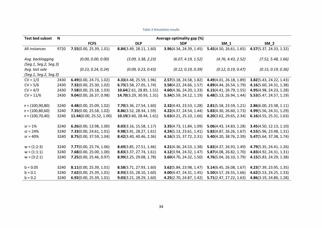
There is also a clear dependency between the resulting average optimality gap and
customer heterogeneity. From Table 3 and the following Figure 2, we observe: (1) In
general, as the scale of customer heterogeneity increases, the performance of all
strategies decreases. (2) Although all strategies show the same increasing pattern as the
scale of customer heterogeneity increases, the performance difference between
strategies is still evident. FCFS is most affected by increasing heterogeneity, followed by
SM_1. On the other hand, the differences between DLP, SM_2 and SDP are rather
constant as heterogeneity increases.
The potential explanation for the first observation might be: When the scale of
customer heterogeneity is small, there is no big difference between customer segments.
Therefore, the cost of “making mistakes” is low. As the scale of customer heterogeneity
increases, the cost of “making mistakes” also increases, which makes larger optimality
gaps.
SDP’s main reaction to the increase of customer heterogeneity is to increase the
segment differentiation, which is reflected in the increasing value of the ratio between
the average service levels of Segment 1 and Segment 3 (third value in parenthesis). This
reaction is reasonable because it is more beneficial to better serve the more profitable
customers when heterogeneity is high. As segment differentiation increases, SDP
backlogs less. This is intuitive: From the average backlogging percentage of each
segment in Table 3 we know that SDP does most of the backlogging for Segment 1 and 2,
because it is only cost-effective to backlog the more profitable customers. As segment
differentiation increases, the more profitable customers are better protected. Therefore,
36
the necessity for backlogging decreases. The increasing segment differentiation and the
decreasing backlogging percentage lead to the increase of the lost sale rate.
Both safety margin models react in the same pattern as the SDP model. However,
the SM_1 model tends to overreact to the heterogeneity increase – when heterogeneity
is low, its ratio between the average service levels of Segment 1 and Segment 3 is
actually small, but the increase of the ratio is much higher than the SDP. This might
explains why its performance deteriorates when heterogeneity is high.
In contrast, DLP has a constant average service level ratio, which means it does not
react to different heterogeneity levels at all.
Figure 2 Average optimality gap for different customer heterogeneity
Supply shortage rate ( )
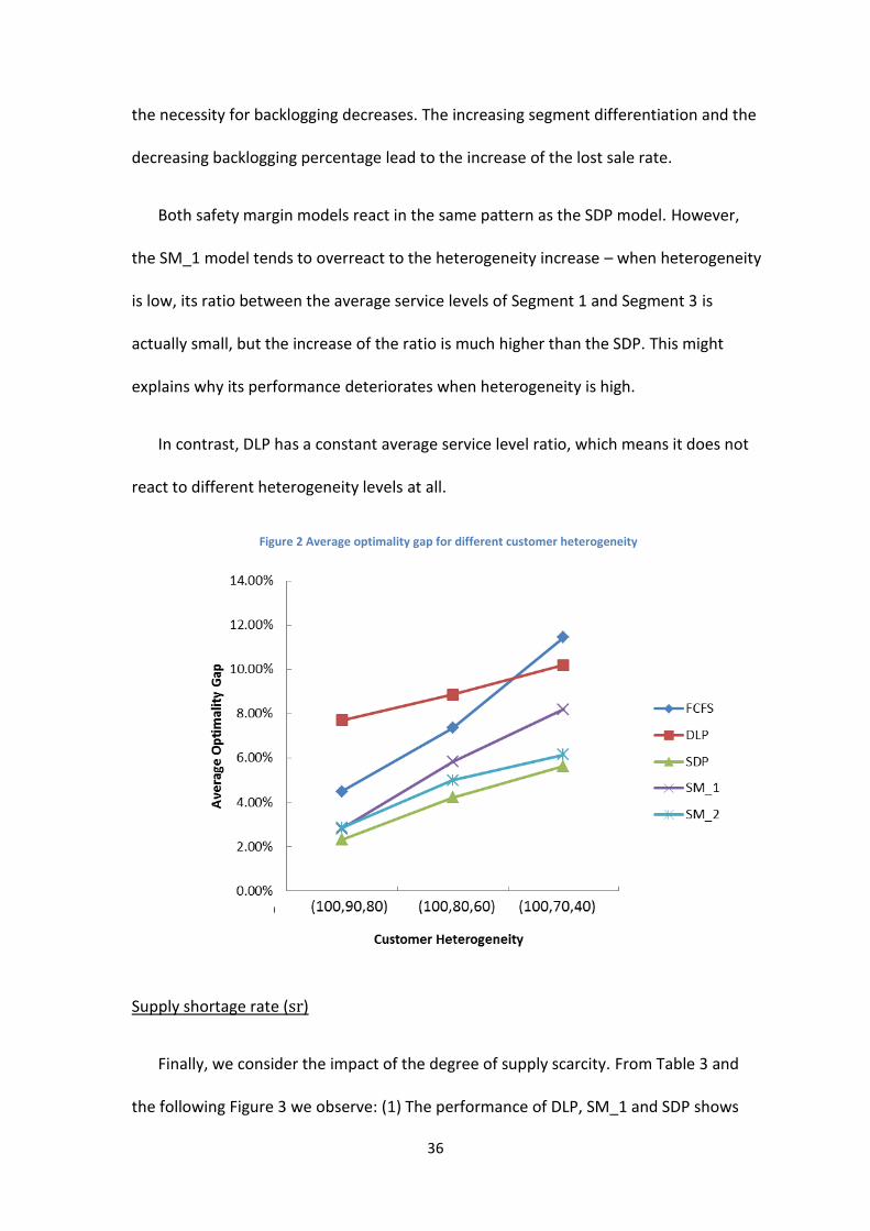
Finally, we consider the impact of the degree of supply scarcity. From Table 3 and
the following Figure 3 we observe: (1) The performance of DLP, SM_1 and SDP shows

37
the same pattern, and it is not monotonic in the shortage rate ( ). All strategies
perform worst for an intermediate shortage rate of 24%. (2) The performance of SM_2
shows a decreasing pattern as the shortage increases.
In response to the increasing shortage, SDP increases its segment differentiation.
This makes sense as it is beneficial to better protect the more profitable customers
when supply is getting scarce. Its backlogging behavior is in line with the average
optimality gap, which is not monotonic in the shortage rate either, and SDP backlogs
most when the shortage rate is 24%. One reasonable explanation is that for an
intermediate shortage rate, the trade-off between selling a unit of supply for current low
revenues versus reserving it for future higher revenues is the most difficult. If shortage is
very low, the solution is clear and simple: to satisfy all the demand from all segments. If
shortage rate is very high, the solution is also obvious: to reserve enough for the more
profitable customers.
The other strategies react in the same way as SDP. However, for SM_2, although it
also increases segment differentiation as shortage rate increases, the extent is not
sufficient. When , SM_2 has nearly the same ratio between the average service
levels of Segment 1 and Segment 3 with SDP. But as the shortage increases, the
difference between the ratios gets larger and larger. When , the average
service level ratio of SM_2 is much lower than SDP. This might explain why the
performance of SM_2 is keeping decreasing when the shortage increases.
38
Figure 3 Average optimality gap for different supply scarcity
39
6. Conclusion and outlook
In this paper, we consider the demand fulfillment problem in make-to-stock
manufacturing where customers are differentiated into different segments based on
their profitability. We follow the two-level planning process of APS and develop two
versions of safety margin model to allocate the pre-determined ATP quantities to
different customer segments with different due date requirement, taking explicitly the
demand uncertainty into account by adding safety margins to the relatively more
profitable customers.
The model is motivated by the observation that the all existing approaches to the
above mentioned demand fulfillment problem have their limitations and could be
further improved. Based on the DLP model from Meyr (2009), we borrow the safety
stock idea from inventory management to account for demand uncertainty and utilize
EMSR to implement it to multi-class case. By doing so, we successfully link the traditional
inventory/supply chain management world to the emerging revenue management world.
The numerical study shows that by incorporating demand uncertainty the safety
margin models do improve the performance of the pure DLP model and provide a close
and efficient approximation to the SDP model which is the optimal ex-ante policy but
computational very expensive. Therefore, we could conclude that our results highlight
the substantial opportunities for improving the demand fulfillment process in make-to-
stock manufacturing and could be easily adapted to the current APS practice.
The main limitation of the safety margin models is that in the allocation stage we
consider the different supplies separately, which results in the over-protection problem
40
for SM_1 and excessive backlogging for SM_2. Besides, there could be other methods to
calculate safety margins, which might improve performance even further. For the
numerical study, a comparison using empirical data instead of theoretical distributions
could provide us further insight into the relative performance of the different policies.