A ROW-WISE STACKING OF THE RUNOFF TRIANGLE: STATE SPACE ...

Astin Bulletin 40(2), 917-946. doi: 10.2143/AST.40.2.2061141 © 2010 by Astin Bulletin. All rights reserved.

A ROW-WISE STACKING OF THE RUNOFF TRIANGLE:STATE SPACE ALTERNATIVES FOR IBNR RESERVE PREDICTION

BY

RODRIGO ATHERINO, ADRIAN PIZZINGA AND CRISTIANO FERNANDES

ABSTRACT

This work deals with prediction of IBNR reserve under a different data ordering of the non-cumulative runoff triangle. The rows of the triangle are stacked, resulting in a univariate time series with several missing values. Under this ordering, two approaches entirely based on state space models and the Kalman fi lter are developed, implemented with two real data sets, and compared with two well-established IBNR estimation methods — the chain ladder and an overdispersed Poisson regression model. The remarks from the empirical results are: (i) computational feasibility and effi ciency; (ii) accuracy improvement for IBNR prediction; and (iii) fl exibility regarding IBNR modeling possibilities.

KEYWORDS

IBNR, Kalman fi lter, mean square error, missing values, state space model.

1. INTRODUCTION

The issue of Incurred But Not Reported (IBNR) reserve prediction has been extensively explored in the actuarial literature. Many techniques have been developed for improving accuracy of the estimated reserves, since biased and unreliable estimation generally result in ineffi cient management decisions(cf. Bornhuetter & Ferguson, 1972). For a good survey on the subject of IBNR estimation, see Taylor (1986), Taylor (2000), England & Verrall (2002), and Tay-lor (2003). In Taylor (2003), the IBNR estimation methods are classifi ed in two different types, namely the static/deterministic and the dynamic/stochastic. The former includes many well-known methods such as the traditional chain ladder, and the latter represents time-varying parameters models, like those dealt with under state space approaches.

This paper suggests a methodology for IBNR prediction which split into two distinct approaches. These should be classifi ed as dynamic/stochastic and are based on an alternative “row-wise” ordering of the values in the runoff triangle. Such ordering produces a univariate time series with several missing

93864_Astin40/2_19.indd 91793864_Astin40/2_19.indd 917 13-12-2010 10:59:0313-12-2010 10:59:03

918 R. ATHERINO, A. PIZZINGA AND C. FERNANDES

values, which, once summed up, give the desired and unobserved IBNR reserve. The approaches that shall be considered are based on state space modeling and the Kalman fi lter, which implies that missing values treatment and mean square error computations become quite attainable.

Even though both approaches give the same numerical result under rather general set-ups, they differ in some aspects. On one hand, the fi rst approach, termed the blocks method, consists of obtaining each “block” of the mean square error matrix associated with the missing values estimates. On the other hand, the second approach, the cumulating method, adds a new component to the state vector, which “accumulates” the missing values estimates and, as a result, the mean square error of the IBNR estimation is automatically obtained from the Kalman equations.

The paper has the following plan. Section 2 presents the notation used through the paper, the proposed new ordering and some justifi cation. Section 3 introduces the essentials of the linear state model and the Kalman fi lter, presents both methodologies in a general framework, and discusses related practical issues. Section 4 is dedicated to applications with two real data sets already used in the literature, where the proposed techniques are estimated, evaluated and compared with the chain ladder method and a Poisson regression model with overdispersion described in Renshaw & Verrall (1998) and England & Verrall (2002); the latter approach has still been quite considered in the litera-ture on IBNR estimation as a standard benchmark — see for instance de Jong (2006). Section 5 concludes the paper and suggests some possible extensions. Technical proofs are relegated to the appendices.

2. THE RUNOFF TRIANGLE: NOTATION AND A NEW ORDERING

Traditionally, IBNR data are organized in the so-called runoff double-index format, as displayed in Figure 1 (see for example Hart et al., 2001). The rows of the triangle represent the accident years or years of origin and its columns give the development years. In this paper, the runoff triangle is portrayed in the incremental form and its cells are denoted by Cwd , 1 ≤ w ≤ J and 0 ≤ d ≤ J – 1; each cell represents, for given w, d, the payment for an accident occurred at time w and reported at time w + d.

A common assumption of several methods for IBNR estimation is the presence of a regular pattern for the incurred liabilities. The pattern originates from the delay between the origin and the payment — that is, a column effect — and should be appropriately modeled and predicted. As a seminal example of this approach, one should recall the Hoerl curve (cf. de Jong & Zehnwirth, 1983; and Wright, 1990). A more recent work from Piet de Jong (cf. de Jong, 2006) focuses on correlations between columns — mainly the earliest ones associated with smaller delays.

In this paper, a different approach is considered. The entries of the triangle in Figure 1 are rearranged as a kind of “time series” formed by stacking the


A ROW-WISE STACKING OF THE RUNOFF TRIANGLE 919

rows, and their former double-index is replaced by a single t, which clearly should not be read as a usual calendar time index. The result is a ordered data set with several missing values — see Figures 2 and 3. Under this new perspec-tive, the dependence structure can be modeled in a natural fashion by a state

AccidentYear

w

Development d

0 1 2 … J – 1

1 C1, 0 C1, 1 C1, 2 … C1, J – 1

2 C2, 0 C2, 1 … C2, J – 2

3 C3, 0 h

h h h

h h CJ – 1, 1

J CJ, 0

FIGURE 1: Runoff Triangle: traditional double-indexing.

AccidentYear

w

Development d

0 1 2 … J – 1

1 y1 y2 y3 … yJ

2 yJ + 1 yJ + 2 … y2J – 1 y2J

3 y2J + 1 y2J + 2 … y3J – 1 y3J

h h h

J y(J – 1) J + 1 y(J – 1) J + 2 … yJ2 – 1 yJ2

FIGURE 2: Row-wise ordering of the triangle.

AccidentYear

w

Development d

0 1 2 … J – 1

1 y1 y2 y3 … yJ

2 yJ + 1 yJ + 2 … y2J – 1

h h

J y(J – 1) J + 1

FIGURE 3: Row-wise ordering of the triangle with missing values.



space framework. A word of caution: even though not having the usual chron-ological meaning, the new index t, instead, offers the possibility of organizing the data following the usual time series analysis standpoint. Besides, it allows the use of periodic components for the aforementioned column effect, as it will be seen in the next section.

Following Figure 1, it should be noted that some entries of Figure 2 are in fact absent, since they correspond to the IBNR components. So, Figure 3 shall be the target of what follows. In practice, to predict the IBNR reserve, which is the unobserved sum given by

tIBNR ,R yt A

/ =!

/ (1)

where A / {t : yt is missing}, means that the missing values of the new repre-sentation must be estimated somehow. It is precisely here where the state space formulation has a major advantage, since missing values treatment is a quite natural task for the Kalman fi lter (cf. Harvey, 1989; Durbin & Koopman, 2001; Brockwell & Davis, 2002; and Shumway & Stoffer, 2006). Besides, as it will be proven in the next section, it will also be possible to obtain an explicit formula for the mean square error of (1) under this proposed new ordering.

3. PROPOSED IBNR ESTIMATION METHODS

3.1. Linear state space models and the Kalman fi lter

A Gaussian linear state space model1 consists of two equations. The fi rst is termed the measurement equation, and describes the evolution of a p-variate observable stochastic process (that is, the measurements) yt, t = 1, 2, …. The second is the state equation. Specifi cally:

yt = Zt at + dt + et , et + N(0, Ht )

at + 1 = Tt at + ct + Rt jt, jt + N(0, Qt ) (2)

a1 + N(a1, P1).

The former equation relates yt to the m ≈ 1 unobserved state at, and the latter gives the state evolution through a Markovian structure. The random errors et and jt are independent (in time, between each other and of a1) and the system matrices Zt, dt, Ht, Tt, ct, Rt and Qt are deterministic. For a given time series of size n and any t, j, defi ne Fj / s(y1, …, yj ), at | j / E(at | Fj ) and Pt | j / Var(at | Fj ).

1 One could think of a wide sense linear state space model, which has no Gaussian assumptions of any kind. Nevertheless, everything developed here maintains great generality, since the formulae corresponding to conditional expectations and covariance matrices still represent, outside Gaussian set-ups, optimal linear estimators and associated mean square error matrices.



The Kalman fi lter (prediction and smoothing equations) consists of recursive equations for these fi rst- and second-order conditional moments when j = t – 1 and j = n. The corresponding expressions are given in (3) and (4). Details concerning the derivations of such formulae and the estimation of unknown parameters in the system matrices by (quasi) maximum likelihood, can be found in several books, like Harvey (1989), Durbin & Koopman (2001), Brock-well & Davis (2002) and Shumway & Stoffer (2006).

ut = yt – Zt at | t – 1 – dt , Ft = Zt Pt | t – 1 Zt� + Ht,

Kt = Tt Pt | t – 1 Zt� Ft –1, Lt = Tt – Kt Zt, t = 1, …, n, (3)

at + 1| t = Tt at | t – 1 + ct + Kt ut, Pt + 1| t = Tt Pt | t – 1 Lt� + Rt Qt Rt�,

rt – 1 = Zt� Ft –1 ut + Lt�rt , Nt – 1 = Zt� Ft

–1 Zt + Lt� Nt Lt ,

at | n = at | t – 1 + Pt | t – 1 rt – 1, Pt | n = Pt | t – 1 – Pt | t – 1 Nt – 1Pt | t – 1, (4)

rn = 0, Nn = 0, t = n, …, 1.

Amongst the works on IBNR estimation employing the state space modeling framework, due attention should be paid to the paper by de Jong & Zehnwirth (1983), who present the triangle of Figure 1 in a way that recognizes the diagonals as the size-varying measurements — consequently, their approach follows the usual calendar time ordering. It is also mentioned that those authors assume a Hoerl Curve structure for each row and its time-varying parameters are the components of the state vector. Verrall (1989), despite of also respecting the usual time frame, considers an estimation method sup-ported by the Bayesian approach; this same inferential perspective was adopted in the work by Ntzoufras & Dellaportas (2002). The class of models proposed by Verrall constitute an adaptation of the static 2-way ANOVA structure of Kremer (1982) to the state space representation. Other works that deserve mentioning are Wright (1990) and Taylor (2003), the latter offer-ing an approach based on the exponential distribution fi lter. More recently, de Jong (2006) proposes a state space form that permits the estimation of correlations between the triangle’s entries. Still, one should recall the book by Taylor (cf. Taylor, 2000), which, amongst many other proposals, discusses a particular method that takes the rows of the runoff triangle as the measurement vectors.

Even though keeping towards an alternative row-ordering of the triangle previously discussed in section 2, the approach of the present paper maintains similarities with the state space proposals of Jong & Zehnwirth (1983) and Taylor (2000), such as introducing structural modeling with stochastic level and periodicity components. The next subsections conserve space to motivate the use of unobserved level and periodic components for probabilistically describing the data in the new row-wise arrangement.



3.2. Structural Models

3.2.1. First proposal

A structural model for a time series has unobservable components, such as level, slope, seasonality and error, which are explicitly modeled (cf. Harvey, 1989). This paper will consider in the applications a structural model with two components: a local level and a stochastic periodic component. It is presented in (5).

yt = mt + gt + xt�b + et, et + N(0, se2 ),

mt + 1 = mt + ht , ht + N(0, sh2 ), (5)

gt + 1 = t j tj

J

11

1w- + -

-

=

g + ,/ wt + N(0, sw2 ).

The use of these components is motivated by the claims process behavior. The basic assumption is that accident years present very similar patterns regarding claims payments, so stacking the whole “square” (that is: the runoff triangle merged with the missing values) as a single univariate time series would generate a very strong periodicity that could be viewed itself as an unobserved stochastic process. As the values of the “lower triangle” are unknown, the time series formed from this new-ordering will have missing values.

Following Harvey (1989 ch. 2), standard structural time series models allow direct interpretation for their unobservable components: the level component responds for long-term movements and the seasonal (periodic) component captures calendar effects. In the present context of runoff data: the level com-ponent mt shall respond for the average value of claims along each accident year, while the periodic component gt is supposed to capture the column effect, already discussed in section 2. The regression terms that appear in the fi rst equation are mainly motivated by the need of intervention effects due to the presence of outliers.

Model (5) is easily cast into a state space form (for example, see Harvey, 1989 ch. 4 and Durbin & Koopman, 2001 ch. 3) and, consequently, everything to be derived in the sequel is certainly applicable. A point is worth stressing: the structural model (5) can also be used with the series in its logged scale, something that maintains coherence with the assumption of the data in its original scale having log-normal distributions. From a purely data-driven per-spective, this way of modeling is generally motivated by residual analysis, whenever the latter suggests a heteroscedastic behavior ex post estimating the model with the original scale. Despite of that, such log-normal distribution is frequently supported in the literature about IBNR data — see subsection 3.3.3. In considering model (5) with logged values, one should, by the time of con-verting the data back to the original scale, be aware of two points: (1) the interpretation for the exponentials of the components shall be multiplicative



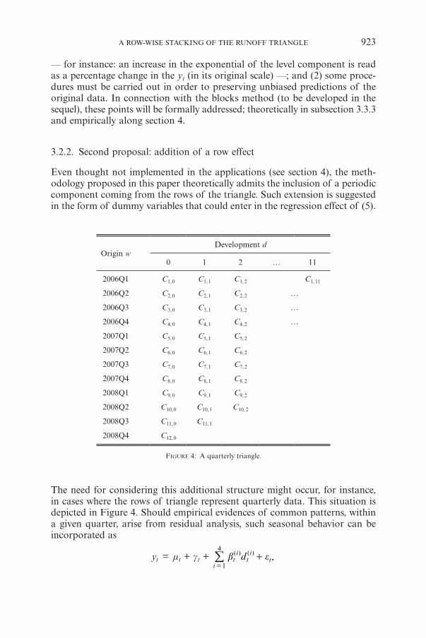
The need for considering this additional structure might occur, for instance, in cases where the rows of triangle represent quarterly data. This situation is depicted in Figure 4. Should empirical evidences of common patterns, within a given quarter, arise from residual analysis, such seasonal behavior can be incorporated as

yt = mt + gt + tt d( (

it

1

4b e+

i i

=

,))/

— for instance: an increase in the exponential of the level component is read as a percentage change in the yt (in its original scale) —; and (2) some proce-dures must be carried out in order to preserving unbiased predictions of the original data. In connection with the blocks method (to be developed in the sequel), these points will be formally addressed; theoretically in subsection 3.3.3 and empirically along section 4.

3.2.2. Second proposal: addition of a row effect

Even thought not implemented in the applications (see section 4), the meth-odology proposed in this paper theoretically admits the inclusion of a periodic component coming from the rows of the triangle. Such extension is suggested in the form of dummy variables that could enter in the regression effect of (5).

Origin wDevelopment d

0 1 2 … 11

2006Q1 C1, 0 C1, 1 C1, 2 C1, 11

2006Q2 C2, 0 C2, 1 C2, 2 …

2006Q3 C3, 0 C3, 1 C3, 2 …

2006Q4 C4, 0 C4, 1 C4, 2 …

2007Q1 C5, 0 C5, 1 C5, 2

2007Q2 C6, 0 C6, 1 C6, 2

2007Q3 C7, 0 C7, 1 C7, 2

2007Q4 C8, 0 C8, 1 C8, 2

2008Q1 C9, 0 C9, 1 C9, 2

2008Q2 C10, 0 C10, 1 C10, 2

2008Q3 C11, 0 C11, 1

2008Q4 C12, 0

FIGURE 4: A quarterly triangle.



where, for each i = 1, …, 4,

tht !

t, quarter

0, otherwised

y1( -=

i ,)

.i"

*,

This extension could be used with types of periodicity others than quarters (e.g. months, semesters etc.). It also worth mentioning that one could con-sider up to S – 1 dummies, where S is the number of row periods, with an intercept term — if S – 1 dummies do enter in the specifi cation, this shall entail an equivalent parametrization to a model with S dummies but with no intercept.

A word of caution: the inclusion of such additional regression terms would certainly turn the maximum likelihood estimation even more diffi cult, given the enormous incidence of missing values (cf. see the discussion concerning the row-wise ordering in section 2).

3.3. First approach: the blocks method

3.3.1. The method

Consider the state space form in (2), the Kalman fi lter in (3) and (4), and all the associated notation and terminology introduced in subsection 3.1. In addition, defi ne I / {t : yt is non- missing}, Y / {ytj

: tj ! I, 6j}, Fu / s(Y) and

t�*

k* *

I*

1� �

t

, if

, otherwise.L

L

TN L L Z F Z L

t

tt

k t

n

k k k k t11

11 1f f/

!

/ += +

- - +* L

t* ** -

* /

In the actual context, Fu represents the information generated by the triangle in Figure 3.

The development of the blocks methods starts from a set of recursions, derived in de Jong & Mackinnon (1988), Koopman (1993) and Durbin & Koopman (2001) ch. 4, for some covariance matrices associated with the error term et and the state vector at. These are collected as follows.

Lemma 1. For any t, j = 1, …, n, it follows that

1. Cov(at, aj | Fn ) = Pt | t – 1 Lt� L�t + 1 … L�j – 1 (Im – Nj – 1 Pj | j – 1 ), j ≥ t

where Lt� L�t + 1 … L�j – 1 = Im for j = t.

2. Cov(et, ej | Fn ) = Ht Kt� L�t + 1 … L�j – 1 Wj�, j > t

where Wj = Hj (Fj – 1Zj – Kj�Nj Lj ).

3. Cov(et, aj | Fn ) = – Ht Kt� L�t + 1 … L�j – 1 (Im – Nj – 1 Pj | j – 1 ), j > t.



4. Cov(at, ej | Fn ) = – Pt | t – 1 Lt� L�t + 1 … L�j – 1Wj�, j ≥ t

where Wj = Hj (Fj – 1Zj – Kj�Nj Lj ) and Lt� L�t + 1 … L�j – 1 = Im for j = t.

Another important result is Lemma 2 given below. Its proof is a direct application of the well-established expressions for the mean vector and the covariance matrix under conditional Gaussian distributions (cf. Johnson & Wichern, 2002).

Lemma 2. Let x, y and z be random vectors with joint Gaussian distribution.If Cov(y, z) = 0 and Cov(x, z) = 0, then

E(x | y, z) = E(x | y)

Var(x | y, z) = Var(x | y).

The next result has a quite direct proof, which is given in appendix A, and reveals a kind of orthogonality between the observed part of the triangle given in Figures 2 and 3, and the IBNR unobserved components.

Lemma 3. For each t " I, et is uncorrelated with Y.

The derivation of the blocks method necessarily passes through the obtention of the conditional covariance matrix of the measurements yt, such that t " I, given the s-fi eld F.u In the actual state space framework, this should be done by considering the conditional covariance matrices between at, et and jt, and by conveniently exploring the linear relation between these unobservable random quantities and the measurements yt. The next result, the proof of which is in appendix B, works out this idea by combining the lemmas already presented in a proper way.

Lemma 4. For each t, j " I, it follows that:

1. j

)=

Cov(,

0, .

for

otherwise

H tFt j

t; =,e e u *

2. Cov (et, aj | Fu ) = 0

3. 1

1 j

jt -

j -)1 =

1

1 1

� � �jCov(

( ),

, .

L L L P for t

N P for t

N <Ft j

t t t t m

t t t t t t

j1 1 1f; =

-

; ;

; ; ;

- + -

- - -

-* * *

jP

P P

*-,

*a

Ia u *

Now, everything needed for the computational expressions of the blocks method has been gathered. These are displayed in the next theorem; proof is given in appendix C:



From a practical/computational perspective, the calculation of the expressions from Theorem 1 needs the storing of several matrices produced by the Kalman fi lter, namely: Pt | t – 1 and N*

t – 1 for each t " I, and also Lt*, L*

t + 1, …, L*t� – 1,

1 ≤ t < t� ≤ n, where t and t� are respectively the fi rst and the last indexes that correspond to missing observations. Additionally, once calculated for each possible combination of i and j, the same expressions give the complete con-ditional covariance matrix of Y / (y1�, …, yn�)� given F.u As a consequence, it turns out to be feasible to compute the mean square error associated with estimation of every linear combination of the missing values — some of which are properly tackled in the next subsection, given their actuarial importance if the missing values do correspond to those from Figure 3.

3.3.2. Mean square error for partial and total IBNR estimation

Since E(a�Y | Fu ) = a�E(Y |Fu ) and Cov(a�Y | Fu ) = a�Cov(Y | Fu ) a for any given vector a = (a1, a2, …, an )�, in order to obtain these statistics for the total IBNR reserve, one must take a such that ai = 1 if i " I and ai = 0 otherwise2. For the partial IBNR reserves, each of these being defi ned as the sum of the entries from a specifi c row of the triangle, one in turn has to fi ll the same vec-tor a with some additional zeros in the appropriate entries. This row-analysis can be useful for identifying some sources of randomness in the components of the IBNR.

Then, the expressions given by the blocks method for the IBNR estimates and their associated standard errors are:

�IBNR E( )aR F;/ = Y u\ (6)

�IBNR sd ( )sd a aR Cov F/ ;= Y u_ ^i h\ (7)

Theorem 1. For each t, j " I, it follows that

j

j

1

1

,

,

and t

t

=t

j

-

-

)

and

1 1 1

1� � �

j

Cov( ( )

( ) .

for t or j

Z N Z H for t j

Z L L L N P Z for t j j

0

<

F

I I

I

I

t j t t t t t t t t t

t t t t t j m1 1 1f

g

g

;

! !

= -; ; ;

; ;

- - -

- + - -* * *

+

j

P P P

P

*

*

�

�-

,y

I

y u

Z

[

\

]]

]]

2 In which concerns a�Cov(Y | Fu ) a, another possibility would be to choose a = (1, …, 1)�, since,theoretically, the multiplications of covariance blocks involving yt , for each t ! I, must vanish(cf. Theorem 1). However, numerically, it is not unreasonable to expect some loss of effi ciency and numerical instability if such parts are not removed from the calculations. These drawbacks are caused by the fact that, although some matrix algebra operations should result in zeros analytically, in practice they do not, in light of rounding errors coming from fl oating point computations (cf. Thisted, 1988).



For the practitioner, the procedure — adapted to the structural modeling framework from subsection 3.2.1 — could be summarized as follows:

1. Estimate the hyperparameters (se2, sh

2 and sw2 ) of the model via maximum

likelihood. If the model has regression parameters, they should be estimated via maximum likelihood as well;

2. Apply the Kalman fi lter given in (3)-(4) and store the matrices Pt | t – 1, Lt and Nt for all t;

3. Construct the covariance matrix Cov(Y | Fu ) using the formulae derived in Theorem 1;

4. Obtain the mean square error of the reserve from (7).

3.3.3. The use of the log-normal distribution for yt

An alternative that has been considered for modeling the runoff data is the log-normal distribution (cf. Taylor, 2000 ch. 9). From the generalized linear modeling perspective, one should look at Kremer (1982), Hertig (1985), Ren-shaw (1989), Christofi des (1990), Verrall (1991), and Doray (1996). Kremer (1982) introduces the 2-way ANOVA to the triangle data, while the others present some variants of the technique or modifi cations on the data perspective, like modeling individual development factors (Hertig, 1985) instead of incremental data. In the time series literature, one should mention the works by de Jong & Zehnwirth (1983), Verrall (1989), de Jong (2004), and de Jong (2006), most of those based on state space models. The log-normal distribution implies an additive structure of the state vector on the logarithmic scale, forcing its com-ponents to be normally distributed.

This alternative distribution induces the following algorithm for estimating the IBNR reserve and calculating its mean square error, which is still entirely supported by the blocks method.

1. Apply the Kalman fi lter to the triangle with entries zt / log yt, storing all the required matrices (see comments coming just after Theorem 1).

2. Use the blocks method to get3 zt / E(zt | Fu ) = E(log yt | Fu ), s2zt /

Var(zt |Fu ) and szt, zj / Cov(zt, zj | Fu ).

3. Compute4:

zt

sy zexp 2t t= +

2

) 3 (8)

y zz

tts s s

t2 1exp t= + e -

2 2 2

z _ i$ . (9)

3 Note that the s-fi elds generated by the original measurements yt and by the transformed measure-ments zt , t ! I, are actually the same.

4 These expression are obtained from a straightforward application of moment generating functions.



j

ysz z

jt zt

s sexp e2 2 1, t

,

t jjs = + + +zy -z

2 2

z_ i* 4 (10)

4. Use the calculations discussed in subsection 3.3.2.

The possibility of adopting the log-normal distribution is a clear advantage of the blocks method over the cumulating method (next section), which does not permit the use of zt.

3.4. Second approach: the cumulating method

3.4.1. The method

The cumulating method consists of plugging a coordinate dt to the state vector in model (2), which shall respond for the accumulation of the estimated missing values. The resulting state space model is

0

p

t

tt

t

t

a

a a

d

T

X I

c R0

0 0

t tt

t t

t

t

t t t1

1

de

d dj

= + +

= + ++

+

,

y Z7 >

> > > > >

A H

H H H H H

(11)

where Xt = 0 for t ! I and Xt = Zt for t " I (missing observation). Also, d1 / 0.

Denote the vector of unknown parameters from models (2) and (11) by c and c† respectively, and the corresponding likelihood functions by L and L †. Although c = c† — indeed: model (11) simply represents an augmentation of the state vector of model (2), whose additional matrices do not bring anynew parameters —, it is not that obvious to affi rm the same, or not, for the maximum likelihood estimators associated with L and L †. The next statement, whose proof is in appendix D, solves the query and shall be key to implementing the method.

Theorem 2. c / arg max L(c) = arg max L †(c†) / c†.

The interpretation of Theorem 2 is that, even though having an additional “cumulating” coordinate in the state vector, the augmented model in (11) does not produce any improvement in the maximum likelihood estimation. In fact, the additional coordinate depends recursively only upon itself, something that preserves the distributional properties of yt. In practice, it shall imply feasibility of the implementations, since the estimation of the unknown parameters can be accomplished using the original model in (2) (which has lower-dimension



matrices) and, after, the obtained estimates should be used with the augmented model in (11).

3.4.2. Extension of the cumulating method: partial and total IBNR estimation

Taking the same motivation given in subsection 3.3.2, it is generally advisable to also incorporate partial cumulating components in the state vector of model (2) for each accident year. Let dt be a J ≈ 1 stochastic process suchdt = (dt

(2), dt(3), …, dt

(J ), dt(T))�, whose indexes (i) represent the entries associated

with each row, the last one being reserved to the total IBNR already defi ned. Use these new quantities, with d1 / 0, to obtain the following model:

t

t I

0(

(

1

1

1+

+

+

t

a

a a

,X

d

T

cR

0 0

0

0

0

0

0

t t

t

t

t t

t

t

t

t

m pJ

pJ pJ

t

tt

t

1

g h

h h hh

d

d

d

e

d

d

d

d

d

d

j

= + +

= + +#

#

+

t

t

t

t

,

(

( (

T

T T

y Z(

( (J J

J

( )

( ) ( )

2

2 2

)

)

)

) )

)

) )

R

T

SSSSSSSSS

R

T

SSSSSSSSS

R

T

SSSSSSSSS

R

T

SSSSSSSSS

R

T

SSSSSS

7

>

V

X

WWWWWWWWW

V

X

WWWWWWWWW

V

X

WWWWWWWWW

V

X

WWWWWWWWW

V

X

WWWWWW

A

H

(12)

where Xt = (Xt(2)�, …, Xt

(J )�, Xt(T )�)�, such that, for each i = 2, …, J,

t

and row

0 otherwiseX

Z t t iIt !

=g

,(i)

*

and also

,

t otherwiseX

t

0

It=

gZT(

.)

)

Clearly, there exists a direct extension of Theorem 2 for model (12) that, again, would serve as a useful device for the estimation of unknown parameters in practical situations.

In which concerns the reserve estimation, by its very defi nition the random vector dJ

2 + 1 has partial and total unobservable IBNR reserves, except for



the system matrices dt and the random errors et, which are excluded from the cumulating process. Therefore, the Kalman fi lter estimates of their entries and the associated mean square errors do play a role in the computations of partial and total IBNR predictions together with their corresponding accuracy meas-ures. For example, the total IBNR estimate and its associated standard error is given by:

d+J 1 tIBNR E( ) ,R Ft I

/ ;d= +g

2T( ) u\ / (13)

+J 1 tsd IBNR sd IBNR ( ) .Var HFt I

/ ;d= +g

2T( ) u_ _i i\ \ / (14)

For the practitioner, the procedure to obtain the mean square errors of the estimated IBNR reserves — under the structural modeling framework from subsection 3.2.1 — is summarized as follows:

1. Estimate the hyperparameters (se2, sh

2, sw2 and the coeffi cients associated

with possible regression terms) of the reduced model by maximum likeli-hood, using the original state space representation (cf. Theorem 2);

2. Apply the Kalman fi lter prediction equations in (3) with extended models of the form given in (12) — the number of cumulating components might depend on the application at hand — and store the result Var(dJ2 + 1 | Fu ).It is the the last block of the matrix PJ2 + 1 | J2 ;

3. Obtain the mean square error of the reserve using (14) and variants for IBNR reserves other than the total.

4. APPLICATIONS

In this section, the methods previously developed are used with two real runoff triangles. The results are compared with those from the traditional chainladder method (CL, hereafter) and those from Renshaw & Verrall (1998) and England & Verrall (2002), who used an overdispersed Poisson regression model (Poisson model, hereafter). In the sequel, the results from the estimations are presented and analyzed. The estimations have been done using a structural time series model as given in (5). The initialization of the Kalman fi lter has been carried out by the exact initial Kalman fi lter as presented in Koopman (1997) and in Durbin & Koopman (2001) ch. 5. The unknown parameters were estimated by maximum likelihood, using the BFGS quasi-Newton optimizer with an aid of the EM algorithm5 in order to obtain good initial guesses for

5 This procedure has been taken in order to alleviate potential problems with the Fisher information due to the missing values, something that usually implies a low curvature of the likelihood function (cf. Migon & Gamerman, 2001 ch. 2).



the variances; see Koopman (1993) and Durbin & Koopman (2001), ch. 7. The state space implementations have been carried out using the Ox 3.0 language (cf. Doornick, 2001) together with the Ssfpack 3.0 library for linear state space modeling (cf. Koopman et al., 2002).

It is also worth mentioning that, although the CL and the Poisson model do incorporate the parameters uncertainty, by considering the modifi cations on the forecast function and on its corresponding mean square error, the approaches proposed in this paper do not. Instead, it was used the very same paradigm defended by Harvey (1989), Brockwell & Davis (1991), Box et al. (1994), Hamilton (1994), Durbin & Koopman (2001), Brockwell & Davis (2002), Enders (2004) and Shumway and Stoffer (2006): expressions for the forecast function and associated mean square error have been derived, and those have been used with maximum likelihood estimates in place of the unknown parameters, resulting in approximated versions of the theoretical formulae.

4.1. AFG data

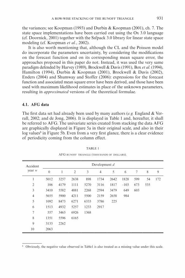
The fi rst data set had already been used by many authors (e.g. England & Ver-rall, 2002; and de Jong, 2006). It is displayed in Table 1 and, hereafter, it shall be referred to AFG. The univariate series created from stacking the data AFG are graphically displayed in Figure 5a in their original scale, and also in their log values6 in Figure 5b. Even from a very fi rst glance, there is a clear evidence of periodicity coming from the column effect.

6 Obviously, the negative value observed in Table1 is also treated as a missing value under this scale.

TABLE 1

AFG RUNOFF TRIANGLE (THOUSANDS OF DOLLARS).

Accidentyear w

Development d

0 1 2 3 4 5 6 7 8 9

1 5012 3257 2638 898 1734 2642 1828 599 54 172

2 106 4179 1111 5270 3116 1817 –103 673 535

3 3410 5582 4881 2268 2594 3479 649 603

4 5655 5900 4211 5500 2159 2658 984

5 1092 8473 6271 6333 3786 225

6 1513 4932 5257 1233 2917

7 557 3463 6926 1368

8 1351 5596 6165

9 3133 2262

10 2063



Given some evidences from residual analysis supporting the presence of outliers, three models have been considered for each of the scales: one withno interventions, other with “less interventions” and another with “more inter-ventions”. These will de referred according to the notation explained below, which also lists the “time instants” that required dummies.

• I-a – original scale with no interventions;• I-b – original scale with 5 interventions (t = 11, 13, 31, 42, 44);

FIGURE 5: AFG time series resulted from row-wise ordering.

0 10 20 30 40 50 60 70 80 90 1000

1000

2000

3000

4000

5000

6000

7000

8000 AFG

0 10 20 30 40 50 60 70 80 90 1004

5

6

7

8

9 Data

5a

5b



• I-c – original scale with 8 interventions (t = 4, 11, 13, 14, 31, 34, 42, 44);• II-a – logarithmic scale with no interventions• II-b – logarithmic scale with 7 interventions (t = 11, 13, 21, 31, 44, 46, 60);• II-c – logarithmic scale with 10 interventions (t = 4, 9, 11, 13, 21, 31, 34, 44,

46, 61);

The estimated variances from the structural model, together with the maximized log-likelihood, are displayed in Table 2, for both original and logarithmic scales. Some complementary information can be extracted from Figures 6 and 7, which contain the output from the Kalman fi lter estimations for models I-c and II-c. The fi rst thing to be noted are the substantial increases in the log-likelihood whenever interventions are added7. These are the very fi rst symp-toms in favor of statistical relevance of such regression terms — there will be certainly more to be said about it later. On the estimated variances and cor-responding signal/noise ratios8, one will probably note that those behave quite differently from one model to another. Although, two points are worth stressing. The fi rst is that, except for model II-a, the periodicity really seems to be sto-chastic, something that is reinforced by the obviously time-varying estimated components depicted in the last panel of Figure 6 and in the second panel of Figure 7. The second is the quite intuitive and therefore expected decreasing path taken by the estimated irregular component variances from model I-a to model I-c (and also from model II-a to model II-c); again, one could take this as another piece of evidence supporting the need of intervening procedures.

In Tables 3, 4 and 5, there are several criteria that are of great help of deciding which model seems to be most appropriate. In the fi rst three lines of

7 Given that some models were estimated with the original data while others used the logged values, the log-likelihoods allowed to be compared are those within a given scale.

8 These are defi ned as the ratios between a level (or periodicity) error variance and the irregular component variance, and, to some extent, reveal the actual importance of such level (or periodicity component) for explaining the movements of the series being modeled.

TABLE 2

ESTIMATED VARIANCES AND SIGNAL-NOISE RATIOS FOR THE AFG DATA.

I-a I-b I-c II-a II-b II-c

Log-likelihood – 407.41 – 392.66 – 380.27 – 62.96 -39.89 – 17.39

Irregular 2.15 ≈ 106 9.89 ≈ 105 3.00 ≈ 105 6.59 ≈ 10 – 1 1.99 ≈ 10 – 1 9.06 ≈ 10 – 187

Level 1.64 ≈ 104 1.03 ≈ 10 – 4 0 1.82 ≈ 10 – 13 9.89 ≈ 10 – 13 1.64 ≈ 10 – 4

Periodic 2.05 ≈ 105 2.37 ≈ 105 3.68 ≈ 105 2.39 ≈ 10 – 10 1.34 ≈ 10 – 2 7.48 ≈ 10 – 2

S/N (level) 7.62 ≈ 10 – 3 1.04 ≈ 10 – 10 0 2.77 ≈ 10 – 13 4.95 ≈ 10 – 12 –

S/N (periodic) 9.55 ≈ 10 – 2 2.39 ≈ 10 – 1 1.23 3.63 ≈ 10 – 10 6.71 ≈ 10 – 2 –



FIGURE 6: Kalman smoothing estimation results from model I-cfor the AFG data in their original scale.

0 10 20 30 40 50 60 70 80 90 1000

250050007500 Data Smoothed Level

0 10 20 30 40 50 60 70 80 90 1000

250050007500 Data Smoothed Forecast

0 10 20 30 40 50 60 70 80 90 100

0

2500

5000 Smoothed Periodicity

FIGURE 7: Kalman smoothing estimation results from model II-cfor the AFG data in their logarithmic scale.

0 20 40 60 80 100456789

10Data Smoothed Level

0 20 40 60 80 100

0

1

2 Smoothed Periodicity

0 20 40 60 80 100456789

10Data Smoothed Forecast (log scale)

0 20 40 60 80 1000

2500

5000

7500

10000 Data Smoothed Forecast (original scale)



Table 3, the in-sample predictive powers of the six proposed models, of the CL and of the Poisson model are assessed using three different performance measures9. Almost all those measures indicate that model I-c compares to models II-c in terms of their best capability of reproducing the data amongst the eight proposals10. Also note that the performance of the CL is quite inferior to all the structural models, even to those that have not accounted for outliers (models I-a and II-a) and that the Poisson model has each of its associated goodness-of-fi t measures assuming values worse than those from the structural models with interventions. Concentrating now on the remaining lines, there are formal and rather strong evidences, gathered from information criteria11

TABLE 3

MODEL COMPARISON STATISTICS ( p-VALUES FOR THE LR TESTS ARE IN PARENTHESES)FOR THE AFG DATA.

I-a I-b I-c II-a II-b II-c CL Poisson

MAPE (%) 52.54 32.55 16.11 59.02 21.29 5.67 ≈ 10 – 16 85.38 65.60

MSE 1.32 ≈ 106 0.60 ≈ 106 0.13 ≈ 106 2.61 ≈ 106 1.18 ≈ 106 1.24 ≈ 10 – 23 3.83 ≈ 106 1.70 ≈ 106

Pseudo R2 (%) 74.26 87.88 97.43 48.63 77.07 99.99 43.22 64.08

AIC 15.29 14.93 14.59 2.76 2.18 1.47 – –

BIC 15.76 15.59 15.36 3.24 2.91 2.31 – –

LR Test – 29.50 54.28 – 46.14 91.14 – –

– (0.000) (0.000) – (0.000) (0.000) – –

TABLE 4

OUT-OF-SAMPLE COMPARISON BETWEEN THE MODELS WITH INTERVENTION FOR THE AFG DATA.

I-a I-b I-c II-a II-b II-c CL Poisson

MAPE (%) 217.40 171.81 156.06 205.72 25.75 19.60 205.17 169.81

MSE 1.60 ≈ 106 0.85 ≈ 106 0.74 ≈ 106 1.97 ≈ 106 0.13 ≈ 106 0.29 ≈ 106 3.92 ≈ 106 1.38 ≈ 106

Pseudo R2 (%) 69.52 80.76 82.34 50.43 96.71 93.29 53.02 63.92

9 During the calculations of these measures, the fi rst row and the fi rst column of the triangle in Table 1 have been discarded, since the former is a diffuse period used to the Kalman fi lter initialization, and the latter cannot be predicted by the CL — in other simple words: only the portion of the data that can be predicted by both the Kalman prediction equations and the CL is considered.

10 Since the variance of the irregular component of model II-c has been estimated to be almost zero — cf. Table 2 —, some care must be exercised in analyzing in-sample measures from this particular model.

11 Same content of footnote 7.



and from likelihood ratio (LR) tests12, in favor of the intervention analyses performed on both original and logarithmic scales.

In Table 4, the structural models, the CL and the Poisson model are con-fronted in an out-of-sample validation. Each of those has been re-estimated without using the diagonal elements of the AFG triangle. Such excludeddata have been compared, by means of the same performance measures, with their corresponding Kalman smoothing out-of-sample estimates. Once more, the CL and the Poisson model were beaten by each of the structural models with interventions and, again, the models that have consistently shown to be the most capable of reproducing the data were I-c and II-c, given their outstanding performances.

12 Here, the null for the LR test is H0 : “The coeffi cients associated with the intervention dummies areall zero”. Consequently, these tests aim at comparing the “reduced” models I-a (II-a) with the “complete” models I-b or I-c (II-b or II-c). Since the required nesting conditions are all respected and both reduced and complete models maintain the standards for good properties of maximum likelihood estimation (cf. Harvey, 1989 sec. 3.4.1 and 4.5.1), it follows that, asymptotically, LR =2[log LMax, Comp – log LMax, Red ] + xk

2 , where k is the number of parameters set to zero under the null. However, analytical and/or Monte Carlo investigations for the LR test about its asymptotic proper-ties would deserve some special attention here, given the amounts of missing values entailed by the approaches of this paper. This important issue shall be left for a future paper. Here, it is a least said that some care has to be taken in forming any judgment from the results of these tests, solely on an asymptotic theory basis.

TABLE 5

DIAGNOSTICS WITH THE STANDARDIZED INNOVATIONS (p-VALUES FOR THE TESTS ARE IN PARENTHESES)FOR THE AFG DATA.

I-a I-b I-c II-a II-b II-c

Heterokedasticity F test (20) 1.225 0.952 1.535 0.589 0.343 1.079

(0.655) (0.913) (0.346) (0.245) (0.021) (0.867)

Ljung-Box autocorrelation test (15 lags) 11.898 8.962 11.660 7.287 12.526 24.530

(standardized innovations) (0.687) (0.879) (0.705) (0.949) (0.639) (0.057)

Ljung-Box autocorrelation test (15 lags) 8.042 7.442 10.411 4.199 9.587 16.690

(squared standardized innovations) (0.922) (0.944) (0.793) (0.997) (0.845) (0.338)

Cox-Stuart independence test 7 6 8 8 7 14

(0.134) (0.052) (0.286) (0.286) (0.134) (0.134)

Jarque-Bera normality test 0.733 1.700 0.486 23.070 13.981 1.569

(0.693) (0.427) (0.784) (0.000) (0.001) (0.456)

Anderson & Darling normality test 0.193 0.328 0.322 0.977 0.685 0.501

(0.890) (0.509) (0.519) (0.013) (0.069) (0.197)

Durbin-Watson 1.778 1.935 2.058 1.639 2.121 2.247

Mean 0.050 0.074 – 0.047 0.104 0.143 – 0.186

Standard deviation 0.999 0.997 0.999 0.995 0.990 0.983



Finally, Table 5 offers diagnostics for the six structural models estimated in this paper. All of them have been performed using the standardized innova-tions, which are defi ned for each t as

Ftt

tu =uS (see subsection 3.1) and, under

the Gaussian state space model basic assumptions, should behave as i.i.d standard normal random variables. Except for model II-b that presents some problems concerning heteroscedasticity — which might imply that most of the remaining diagnostics for this specifi c model turn meaningless —, and for model II-a that had a relatively low Durbin-Watson statistic and showed an expressive lack of normality behavior (see small p-values for its corresponding Jarque-Bera and Anderson-Darling tests), all the basic assumptions are being fairly supported by the data, including the cases of models I-c and II-c (with “more interventions”) that gave the best data fi ts. Still concerning these two models, Figures 8 and 9 serve as additional information that indicates excellent behavior of their standardized innovations and auxiliary residuals, the latter of which constituting an important tool for identifying remaining outliers13 (cf. Durbin & Koopman, 2001 ch. 7).

The total and partial IBNR estimated reserves are given in Table 6 along with their corresponding theoretical coeffi cients of variation (CV). The con-struction of such theoretical predictive measure has been made possible by the block method from section 3.3 applied to the structural models I-c and II-c, by Mack’s approach for the CL (cf. Mack 1993, 1994a and 1994b) and by the formulae derived in Renshaw & Verrall (1998) and England & Verrall (2002) for the Poisson model14. From a perspective widely adopted in the literature, which bases itself on the comparison of CVs from different methods, it is unlikely to expect any conclusion different from the following:

• in which concerns total IBNR estimation, model I-c gave better results as compared with the CL, the Poisson model and model II-c.

• in which concerns partial IBNR estimation, the CL and the Poisson model at times outperform model I-c.

While the fi rst conclusion is in some tune with previous analyses, the second goes in an opposite direction. In addition, it is worth stressing that, even though omitted to conserve space, additional CV comparisons taking account models I-a, I-b, II-a and II-b did support some models already proved to be not the most suitable choices for describing the AFG data. Quick example: model II-b showed a heteroscedastic behavior in its standardized innovation (see Table 5), besides offering less predictive power than model II-c (see Table 3); however, for the total IBNR estimation, the CV of the former was 14.8%, against 17.1% of the latter.

13 The analysis is as follow: if an observed auxiliary residual is larger than 3 in absolute value, one should take this as an evidence in favor of an outlier.

14 Formal justifi cation for using the Poisson distribution with claims amounts and a technical discus-sion about the numerical coincidence between the estimated reserves from the CL and from the Poisson model is offered in Renshaw & Verrall (1998).



FIGURE 8: Diagnostics from model I-c for the AFG data in their original scale.

0 20 40 60 80 100

012 Standardized innovation

0 20 40 60 80 100

012 Auxiliary residual

0 5 10 15 20

0

1

0 5 10 15 20

0

1

0 1 2

0.2

0.4 N(s=0.999)

0 1 2

0

2 Standardized Innovation × normal

FIGURE 9: Diagnostics from model II-c for the AFG data in their logarithmic scale.

0 20 40 60 80 100

0

2Standardized innovation

0 20 40 60 80 100

Auxiliary residual

0 10 20

0

1

0 10 20

0

1

0 1 2 3

2

4

6

0 1

0

2 Standardized Innovation × normal



In light of these confronting conclusions, some questioning should be posed about the use of the CV to evaluate alternatives for IBNR estimation. Indeed, one should bear in mind that this measure is obtained using some theoretical formulae derived from the model being considered and, as such, needs not be supported anyhow by the data. If, for instance, a given model violates some basic assumptions or does not suitably predict/reproduce the data, then, rigorously speaking, there might not be many arguments left in favor of trusting on theoretical measures, such as the CV, computed under misspecifi ed hypotheses. Consequently, this paper defends that theoretical measures, like the mean square errors from the block and cumulating methods and their resulting CVs, must not be evoked as complementary criteria for model selection, but, instead, should be used for assessing the nominal predic-tive power and reduced uncertainty implied by the “best” models.

4.2. MC1 data

The second runoff triangle chosen to be tested with the approaches of this paper is displayed in Table 7 and had been previously considered by Verral (1991) and Mack (1993). It shall be referred to MC1.

In order to conserve space and since the modeling strategies have proved to be quite the same of those adopted with the AFG data, this subsection will focus on showing only the summary results. The best structural model forthe MC1 was one estimated with the data in their logarithm scale and had 10 intervention dummies for outliers that appeared in t = 4, 6, 7, 14, 17, 26, 27, 34,25, 73; such terms have shown to be statistically signifi cant by the same LR test used with the AFG data. In Table 8, this model is compared with the CL

TABLE 6

ESTIMATED RESERVES FOR THE AFG DATA AND CORRESPONDING COEFFICIENTS OF VARIATIONS

(IN PARENTHESES).

Accident year Chain ladder Poisson Model I-c Model II-c

2 154 (134.0%) 154 (361%) 226 (461.5%) 199.57 (24.0%)

3 617 (101.0%) 617 (181%) 1185.09 (112.4%) 937.43 (22.1%)

4 1636 (45.7%) 1636 (109%) 2264.32 (67.3%) 1597.49 (20.9%)

5 2747 (53.5%) 2747 (81%) 4118.51 (40.5%) 2733.11 (19.4%)

6 3649 (54.9%) 3649 (67%) 5544.08 (32.2%) 5836.64 (18.4%)

7 5435 (40.6%) 5435 (57%) 8270.34 (22.7%) 9046.18 (18.7%)

8 10907 (49.1%) 10907 (46%) 9286.14 (21.1%) 11051.12 (22.2%)

9 10650 (59.5%) 10650 (57%) 16435.9 (12.4%) 20882.02 (20.8%)

10 16339 (150.4%) 16339 (79%) 19525.93 (10.9%) 25393.56 (25.2%)

Total 52135 (51.6%) 52135 (35%) 66856.31 (14.9%) 77677.13 (17.1%)



and the Poisson model in terms of in-sample and out-of sample predictive measures. From those fi gures, it is clear that the structural model has once more shown to be superior to its competing approaches, from both in-sample and out-of-sample standpoints.

Table 9 gives the fi nal IBNR estimates, which resulted from an application of the blocks method related formula (8), discussed in subsection 3.3.3. As can readily seen, the CL and the Poisson model tend to systematically give reserves larger than those obtained from the structural model, the exception being only the partial IBNR reserve associated with the 10th accident year. Should the CL and/or the Poisson model be in fact not adequate methods to estimate the reserve, and should the structural model be a valid probabilistic description of the true data generating mechanism — two conjectures fairly supported by the

TABLE 7

MC1 RUNOFF TRIANGLE.

Accident year

w

Development d

0 1 2 3 4 5 6 7 8 9

1 357848 766940 610542 482940 527326 574398 146342 139950 227229 67948

2 352118 884021 933894 1183289 445745 320996 527804 266172 425046

3 290507 1001799 926219 1016654 750816 146922 495992 280405

4 310608 1108250 776189 1562400 272482 352053 206286

5 443160 693190 991983 769488 504851 470639

6 396132 937085 847498 805037 705960

7 440832 847631 1131398 1063269

8 359480 1061648 1443370

9 376686 986608

10 344014

TABLE 8

MODEL COMPARISON STATISTICS FOR THE MC1 DATA.

Structural model CL Poisson

MAPE in-sample (%) 10.31 28.84 23.32

MSE in-sample 0.87 ≈ 1010 4.42 ≈ 1010 2.50 ≈ 1010

Pseudo R2 in-sample (%) 92.95 63.46 79.37

MAPE out-of-sample (%) 17.75 24.08 20.29

MSE out-of-sample 1.27 ≈ 1010 2.89 ≈ 1010 1.42 ≈ 1010

Pseudo R2 out-of-sample (%) 97.91 87.28 93.40



data in view of the results concerning predictive power —, a insurance com-pany would have incurred the risk of loosing competitiveness if the CL or the Poisson model results were taken as the fi nal ones.

Finally, a word about the theoretical accuracy measures from both approaches is pertinent. From Table 9, one can easily notice that every reported CV from the CL and from the Poisson model is larger than its corresponding one asso-ciated with the structural model, the latter being obtained from Theorem 1 with an aid from formulae (9) and (10) from subsection 3.3.3. Sticking to the standpoints proposed and supported in the fi nal of subsection 4.1, this fi nding must not be interpreted in this paper as another piece of evidence of a better predictive capability for the structural model. Instead, the CVs associated with the structural model are considered to be the “most correct”, in light of the data analyses that generated the results and suggested inadequacy of the CL and of the Poisson model.

5. CONCLUSION

The empirical evidences from section 4 suggest that the alternative ordering of the runoff triangle and the proposed techniques of this paper emerge as useful alternatives for IBNR prediction. Another interesting point is the pos-sibility of choosing from two different methods (blocks or cumulating), whose fi nal results are guaranteed to be the same, should one consider the data in their original scale. Also, from the computational standpoint, the models pro-posed are quite tractable, since the methodological basis given by the Kalman fi ltering is rather effi cient nowadays. Finally, since everything developed here

TABLE 9

ESTIMATED RESERVES FOR THE MC1 DATA AND CORRESPONDING COEFFICIENTS OF VARIATIONS

(IN PARENTHESES).

Accident year CL Poisson Structural model

2 94,634 (79.8%) 94,634 (116.3%) 78,904 (23.3%)

3 469,510 (25.9%) 469,511 (46.0%) 433,790 (17.3%)

4 709,640 (18.8%) 709,638 (36.8%) 663,310 (13.7%)

5 984,890 (26.5%) 984,889 (30.8%) 891,770 (12.0%)

6 1,419,500 (29.0%) 1,419,459 (26.4%) 1,336,400 (10.8%)

7 2,177,600 (25.6%) 2,177,640 (22.7%) 2,009,900 (10.3%)

8 3,920,300 (22.3%) 3,920,301 (20.2%) 2,919,600 (10.4%)

9 4,279,000 (22.7%) 4,278,972 (24.5%) 3,810,800 (10.8%)

10 4,625,800 (29.5%) 4,625,810 (42.8%) 4,726,900 (12.1%)

Total 18,681,000 (13.1%) 18,680,854 (15.8%) 16,871,000 (7.1%)



is embedded in a linear state space framework, there is still the great fl exibility of considering a wider range of statistical models for IBNR data.

This paper closes with four perspectives for future research:

• The fi rst is a Monte Carlo study for assessing the small sample statistical properties of the LR tests used here for the intervention effects, since this papers’s ordering of IBNR data always induces a small time series with lots of missing values. Besides, according to many other practical experiences, it is not unusual to fi nd outliers in runoff data sets, and it is surely advisable to use signifi cance tests for the inclusion of intervention dummies.

• The second suggestion is to consider other frameworks in state space mode-ling, such as non-Gaussian possibilities. For instance, one could understand that the numbers of outliers from the best models in both applications of the paper exceeded reasonable limits, which would serve as evidence in favor of heavy-tailed distributions. However, one must be aware of the complications of taking this path, since, as regards the alternatives for estimating more gen-eral state space models, none of them is computationally trivial — see for instance the importance sampling approach by Durbin and Koopman (2001) Part II, the particle fi lters developed along the chapters of Doucet et al. (2001) and the density – based nonlinear fi lters in Tanizaki (1996) ch. 4.

• Thirdly, we mention that, should a formal justifi cation become available, an extension of the structural model (5) in which the level and the periodic com-ponents are dependent can be a valid alternative. But, as just said, the ques-tion that might be answered before considering such more complex modeling alternative — which might probably entail numerical diffi culties even greater than the existing ones — is: are there any previous experiences or actuarial theories suggesting that the average value of claims along each accident year (supposed to be represented by the level component mt) and the values associ-ated with each delay time between the origin and the payment (supposed to be represented by the periodic component gt) could interact anyhow?

• Finally, the fourth possibility, which shall be certainly relevant if one con-siders the use of such methods in an insurance company, would be the study about how different initializations of the Kalman recursions affect fi nal IBNR predictions and associated mean square errors.

6. ACKNOWLEDGEMENTS

Two anonymous Referees and the Editor Michel Denuit have greatly contributed with their suggestions, corrections and requirements for improving the paper. The authors are grateful to Andrew C. Harvey for his constructive comments and suggestions, particularly those initial ideas that have inspired the whole section 3.4. The suggestions and corrections from Kaizo Beltrao, Nei Carlos Rocha, Marcelo Medeiros and Alvaro Veiga were also of great value for improving the paper. The fi rst author is grateful to the CNPq. The second author acknowledges support from the FAPERJ (PDR scholarship).



APPENDIX

A. Proof of Lemma 3

Fix an arbitrary t " I. It is suffi cient to prove that Cov(et, ys) = 0, for each s ! I. But this follows from the recursive solution of the measurement equation, which is

Tj Rk +jjay Z T c ds sj

s

k j

s

j

s

j s s s t s1

1

11

1

1

2

1 1 1j e= + + + +=

-

= +

-

=

-

- - -+R c ,j_ i> >H H* 4% %/

and from the random vectors et, es, jj for j = 1, …, s – 1 and a1 being mutually uncorrelated (cf. assumptions listed in subsection 3.1). ¡

B. Proof of Lemma 4

Consider an auxiliary linear state space model that has the same state equation of (2) and whose measurement equation is given by

yt* = Zt

*at + dt* + et

*, et* + N(0, Ht

*),

where yt* = yt, Zt

* = Zt, dt* = dt and Ht

* = Ht for t ! I, and Zt* = 0, dt

* = 0 and Ht

* = I otherwise. Therefore, once ys* is uncorrelated with (Y�, at�, ej�)� for

s, t, j " I, expression 1 follows from Lemmas 2 and 3 (indeed: under normality, absence of correlation implies independence), and expressions 2 and 3 are direct consequences from Lemmas 2 and 1, noting once more that Ki = 0 whenever i " I. ¡

C. Proof of Theorem 1

If t ! I, then E(yt | Fu ) = yt , which is suffi cient for the fi rst case. Now, suppose that t, j " I and note that, from the measurement equation of (2),

�

�.

+Cov( | ) Cov( | ) Cov( | )

Cov( | ) Cov( | )

Z

Z

F F F

F F

t j t t j j t j

t t j t j j

=

+ +

a

a

e, , ,

,

e

e ,

a

a

y

e

y Z

Z

u u u

u u (15)

From item 2 of Lemma 4, the third and fourth terms from right-hand of (15) vanish. Besides, if t = j, items 1 and 3 from Lemma 4 assert that the fi rst and second terms from right-hand of (15) result in Zt (Pt | t – 1 – Pt | t – 1 N*

t – 1 Pt | t – 1) Zt� and Ht, respectively. This proves the second case. Finally, if t < j, then, again from items 1 e 3 of Lemma 4, the fi rst term from right-hand of (15) equals

1j -1� � �

j t( )Z L L L N P Zt t t t t j m1 1 1f; ;- + - -

* * *j

�P *-I and the second vanishes, proving the third case. ¡



D. Proof of Theorem 2

It is suffi cient to prove that L = L† over all the parametric space, which, in light of the prediction error decomposition of the likelihood (cf. Harvey, 1989), comes as a consequence of showing that ut = ut

† for each t = 1, …, n. Implementing: fi x an arbitrary t. According to (3) applied to models (2) and (11), it follows that

ut = yt – Zt at | t – 1 – dt and ut† = yt

† – Zt a†t | t – 1 – dt , (16)

where “†” is an indication that the model under consideration is the augmented and a†

t | t – 1 / E(at | F †t – 1 ). Besides, under the augmented model in (11), the recur-sive solution for the measurement equation, for an arbitrary s = 1, …, t – 1, is

spp

0

0

ja

.

yII

R c

c Rd

00

0 0

0 0

s

s

s

k

kk j

j

jj

s

j

s jj

s ss s s

1

11

1 1

1 1

2

1 11

d

j e

=

+

+ + +

+ + +

-

= +=

-

=

-

- -

-

@ jZT

X

Z

T

Xf p7 >> > >> > >

7 > >

A HH H HH H H

A H H

*

*

4

4

%% /

(17)

Observe that

p p

Tj 1=

I I

0 0j

jj

sj

s

s1

11

==

--

A

T

X> >H H%

% (18)

and

p

j j

j

kj j,

I

R c T R c

B

0

0 0

k

kk j

s

j

s

jk js

j

s

1

1

1

21

1

1

2+ =

+

= +

-

=

-= +

-

=

- jj

T

X

jf

_p

i>> > > >HH H H H%

%/ / (19)

where As depends upon Zj and Tj, j = 1, …, s – 2, and the matrices Bj depend upon Zk and Tk, k = j + 1, …, s – 2. Then, placing (18) and (19) appropriately in (17) implies

s RjTT s 1 +-( )y Z c c ds jj

s

j kj

s

j j s sj

s

t s1

1

1

1

1 11

2j e= + + + + +

=

-

=

-

- -=

-@ ,R ja= =G G* 4% %/ (20)

which coincides with the recursive solution of the measurement equation from the original model (2). Finally, combine (20) and (16). ¡



REFERENCES

BORNHUETTER, R. and FERGUSON, R. (1972) The Actuary and IBNR. Proceedings of the Casu-alty Actuarial Society, 59, 181-195.

BOX, G., JENKINS, G. and REINSEL, G. (1994) Time Series Analysis, Forecasting and Control. 3rd edi-tion. Holden-Day.

BROCKWELL, P.J. and DAVIS, R.A. (1991) Time Series: Theory and Methods. 2nd edition. Springer-Verlag.

BROCKWELL, P.J. and DAVIS, R.A. (2002) Introduction to Time Series and Forecasting. Springer.CHRISTOFIDES, S. (1990) Regression models based on log-incremental payments. Claims Reserving

Manual, Vol. 2. Institute of Actuaries.DE JONG, P. (2004) Forecasting general insurance liabilities. Technical report, Macquarie Univer-

sity. Department of Actuarial Studies Research Paper Series.DE JONG, P. (2006) Forecasting runoff triangles. North American Actuarial Journal, 10(2), 28-38.DE JONG, P. and ZEHNWIRTH, B. (1983) Claims reserving, state-space models and the Kalman

fi lter. Journal of the Institute of Actuaries, 110, 157-181.DE JONG, P. and MACKINNON, M. (1988) Covariances for smoothed estimates in state space

models. Biometrika, 75(3), 601-602.DOORNICK, J.A. (2001) Ox 3.0: An Object-Oriented Matrix Programming Language. Timberlake

Consultants LTD.DORAY, L.G. (1996) Umvue of the ibnr reserve in a lognormal linear regression model. Insurance:

Mathematics and Economics, 18, 43-57.DOUCET, A., FREITAS, N. and GORDON, N. (2001) Sequential Monte Carlo Methods in Practice.

Springer.DURBIN, J. and KOOPMAN, S.J. (2001) Time Series Analysis by State Space Methods. Oxford

Statistical Science Series.ENDERS, W. (2004) Applied Econometric Time Series. 2nd edition. John Wiley & Sons.ENGLAND, P.D. and VERRALL, R.J. (2002) Stochastic claims reserving in general insurance. Jour-

nal of the Institute of Actuaries, 129, 1-76.HAMILTON, J.D. (1994) Time Series Analysis. Princeton University Press.HART, D., BUCHANAN, R. and HOWE, B. (1996) The Actuarial Practice of General Insurance.

Institute of Actuaries of Australia.HARVEY, A.C. (1989) Forecasting, Structural Time Series Models and the Kalman Filter. Cam-

bridge University Press.HERTIG, J. (1985) A statistical approach to the ibnr-reserves in marine insurance. ASTIN Bul-

letin, 15, 171-183.JOHNSON, R. and WICHERN, D. (2002) Applied Multivariate Statistical Analysis. 5th edition.

Prentice Hall.KOOPMAN, S.J. (1993) Disturbance smoother fo state space models. Biometrika, 80(1), 117-126.KOOPMAN, S.J. (1997) Exact Initial Kalman Filtering and Smoothing for Nonstationary Time

Series Models. Journal of the American Statistical Association, 92, 1630-1638.KOOPMAN, S.J., SHEPHARD, N. and DOORNIK, J.A. (2002) SsfPack 3.0 beta02: Statistical algorithms

for models in state space. Unpublished paper. Department of Econometrics, Free University, Amsterdam.

KREMER, E. (1982) Ibnr claims and the two-way model of anova. Scandinavian Actuarial Journal.MACK, T. (1993) Distribution-free calculation of the standard error of chain ladder reserve

estimates. ASTIN Bulletin, 23(2), 213-225.MACK, T. (1994a) Which stochastic model is underlying the chain ladder method? Insurance:

Mathematics and Economics, 15, 133-138.MACK, T. (1994b) Measuring the variability of chain ladder reserve estimates. Casualty Actuarial

Society Spring Forum, 101-182.MIGON, H. and GAMERMAN, D. (1999) Statistical Inference: an Integrated Approach. A Hodder

Arnold Publication.NTZOUFRAS, I. and DELLAPORTAS, P. (2002) Bayesian Modelling of Outstanding Liabilities Incor-

porating Claim Count Uncertainty. North American Actuarial Journal, 6(1), 113-136.RENSHAW, A.E. (1989) Chain ladder and interactive modelling (claims reserving and glim). Jour-

nal of the Institute of Actuaries, 116, 559-587.



RENSHAW, A.E. and VERRALL, R.J. (1998) A stochastic model underlying the chain-ladder technique. British Actuarial Journal, 4(4), 903-923.

SCHNIEPER, R. (1991) Separating true ibnr and ibner claims. ASTIN Bulletin, 21(1).SHUMWAY, R.H. and STOFFER, D.S. (2006) Time Series Analysis and Its Applications (With R

Examples). 2nd edition. Springer.TANIZAKI, H. (1996) Nonlinear Filters. 2nd edition. Springer.TAYLOR, G. (1986) Claims Reserving in Non-Life Insurance. North-Holland.TAYLOR, G. (2000) Loss Reserving: an Actuarial Perspective. Springer.TAYLOR, G. (2003) Loss reserving: Past, present and future. Research Paper no. 109, The Univer-

sity of Melbourne.THISTED, R.A. (1988) Elements of Statistical Computing: Numerical Computation. Chapman &

Hall.VERRALL, R. (1989) State space representation of the chain ladder linear model. Journal of the

Institute of Actuaries, 116, 589-610.VERRALL, R. (1991) On the estimation of reserves from loglinear models. Insurance: Mathematics

and Economics, 10, 75-80.WRIGHT, T. (1990) A stochastic method for claims reserving in general insurance. Journal of the

Institute of Actuaries, 117, 677-731.

ADRIAN PIZZINGA (Corresponding author)Department of Statistics – Institute of Mathematics and StatisticsFluminense Federal University (UFF)Campus do Valonguinho – CentroRua Mario Santos Braga, s/n – 7° andar24020-140 Niterói – Rio de JaneiroBrazilE-mail: [email protected]

[email protected]

RODRIGO ATHERINO JGP Global Gestao de RecursosDepartment of Electrical EngineeringPontifi cal Catholic University of Rio de Janeiro.

CRISTIANO FERNANDES Department of Electrical EngineeringPontifi cal Catholic University of Rio de Janeiro.


A ROW-WISE STACKING OF THE RUNOFF TRIANGLE: STATE SPACE ...

Documents

Transcript of A ROW-WISE STACKING OF THE RUNOFF TRIANGLE: STATE SPACE ...