http://sites.uclouvain.be/absil/2013.03 Tech. report UCL-INMA-2013.03-v1

A Riemannian symmetric rank-one trust-region method∗

Wen Huang† P.-A. Absil‡§ K. A. Gallivan†

April 18, 2013

Abstract

The well-known symmetric rank-one trust-region method—where the Hessian approximationis generated by the symmetric rank-one update—is generalized to the problem of minimizinga real-valued function over a d-dimensional Riemannian manifold. The generalization relieson basic differential-geometric concepts, such as tangent spaces, Riemannian metrics, and theRiemannian gradient, as well as on the more recent notions of (first-order) retraction and vectortransport. The new method, called RTR-SR1, is shown to converge globally and d + 1-step q-superlinearly to stationary points of the objective function. A limited-memory version, referredto as LRTR-SR1, is also introduced. In this context, novel efficient strategies are presented toconstruct a vector transport on a submanifold of a Euclidean space. Numerical experiments—Rayleigh quotient minimization on the sphere and a joint diagonalization problem on the Stiefelmanifold—illustrate the value of the new methods.

Key words: Riemannian optimization; optimization on manifolds; SR1 trust-region; sym-metric rank-one update; vector transport; Rayleigh quotient; joint diagonalization; simultaneousdiagonalization; Stiefel manifold

2010 Mathematics Subject Classification: 65K05, 90C48, 90C53

1 Introduction

We consider the problemminx∈M

f(x) (1)

of minimizing a smooth real-valued function f defined on a Riemannian manifold M. Recentlyinvestigated application areas include image segmentation [RW12] and recognition [TVSC11], elec-trostatics and electronic structure calculation [WY12], finance and chemistry [Bor12], multilinear

∗This paper presents research results of the Belgian Network DYSCO (Dynamical Systems, Control, and Opti-mization), funded by the Interuniversity Attraction Poles Programme initiated by the Belgian Science Policy Office.This work was financially supported by the Belgian FRFC (Fonds de la Recherche Fondamentale Collective). Thiswork was performed in part while the third author was a Visiting Professor at the Institut de mathematiques pureset appliquees (MAPA) at Universite catholique de Louvain.

†Department of Mathematics, 208 Love Building, 1017 Academic Way, Florida State University, Tallahassee FL32306-4510, USA

‡Department of Mathematical Engineering, ICTEAM Institute, Universite catholique de Louvain, B-1348 Louvain-la-Neuve, Belgium

§Corresponding author. URL: http://sites.uclouvain.be/absil/ Phone: +32-10-472597. Fax: +32-10-472180.

1

algebra [SL10, IAVD11], low-rank learning [MMBS11, BA11], and blind source separation [KS12,SAG+12].

The wealth of applications has stimulated the development of general-purpose methods for (1)—see, e.g., [AMS08, RW12, SI13] and references therein—including the trust-region approach uponwhich we focus in this work. A well-known technique in optimization [CGT00], the trust-regionmethod was extended to Riemannian manifolds in [ABG07] (or see [AMS08, Ch. 7]), and foundapplications, e.g., in [JBAS10, VV10, IAVD11, MMBS11, BA11]. Trust-region methods constructa quadratic model mk of the objective function f around the current iterate xk and produce acandidate new iterate by (approximately) minimizing the model mk within a region where it is“trusted”. Depending on the discrepancy between f and mk at the candidate new iterate, the sizethe of trust region is updated and the candidate new iterate is accepted or rejected.

For lack of efficient techniques to produce a second-order term in mk that is inexact but nev-ertheless guarantees superlinear convergence, the Riemannian trust-region (RTR) framework losessome of its appeal when the exact second-order term—the Hessian of f—is not available. This isin contrast with the Euclidean case, where several strategies exist to build an inexact second-orderterm that preserves superlinear convergence of the trust-region method. Among these strategies,the symmetric rank-one (SR1) update is favored in view of its simplicity and because it preservessymmetry without unnecessarily enforcing positive definiteness; see, e.g., [NW06, §6.2] for a moredetailed discussion. The n+1 step q-superlinear rate of convergence of the SR1 trust-region methodwas shown by Byrd et al. [BKS96] using a sophisticated analysis that builds on [CGT91, KBS93].

In this paper, motivated by the situation described above, we introduce a generalization of theclassical (i.e., Euclidean) SR1 trust-region method to the Riemannian setting (1). Besides makinguse of basic Riemannian geometric concepts (tangent space, Riemannian metric, gradient), thenew method, called RTR-SR1, relies on the notions of retraction and vector transport introducedin [ADM+02, AMS08]. A detailed global and local convergence analysis is given. A limited-memoryversion of RTR-SR1, referred to as LRTR-SR1, is also introduced. Numerical experiments showthat the RTR-SR1 method displays the expected convergence properties. When the Hessian of fis not available, RTR-SR1 thus offers an attractive way of tackling (1) by a trust-region approach.Moreover, even when the Hessian of f is available, making use of it can be numerically expensive,and the numerical experiments show that ignoring the Hessian information and resorting insteadto the RTR-SR1 approach can be beneficial.

Another contribution of this paper with respect to [BKS96] is an extension of the analysis toallow for inexact solutions of the trust-region subproblem—compare (9) with [BKS96, (2.4)]. Thisextension makes it possible to resort to inner iterations such as the Steihaug–Toint truncated CGmethod (see [AMS08, §7.3.2] for its Riemannian extension) while staying within the assumptionsof the convergence analysis.

The paper is organized as follows. The RTR-SR1 method is stated and discussed in Section 2.The convergence analysis is carried out in Section 3. The limited-memory version is introduced inSection 4. Numerical experiments are reported in Section 5. Conclusions are drawn in Section 6.

2 The Riemannian SR1 trust-region method

The proposed Riemannian SR1 trust-region (RTR-SR1) method is described in Algorithm 1. Thealgorithm statement is commented in Section 2.1 and the important questions of representingtangent vectors and choosing the vector transport are discussed in Sections 2.2 and 2.3.

2

Algorithm 1 Riemannian trust region with symmetric rank-one update (RTR-SR1)

Input: Riemannian manifoldM with Riemannian metric g; retraction R; isometric vector trans-port TS ; differentiable real-valued objective function f on M; initial iterate x0 ∈ M; initialHessian approximation B0, symmetric with respect to g.

1: Choose ∆0 > 0, ν ∈ (0, 1), c ∈ (0, 0.1), τ1 ∈ (0, 1) and τ2 > 1; Set k ← 0;2: Obtain sk ∈ Txk

M by (approximately) solving

sk = arg mins∈Txk

Mmk(s) = arg min

s∈TxkM

f(xk) + g(grad f(xk), s) +1

2g(s,Bks), s.t. ‖s‖ ≤ ∆k; (2)

3: Set ρk ←f(xk)−f(Rxk

(sk))

mk(0)−mk(sk);

4: Let yk = T −1Sskgrad f(Rxk

(sk)) − grad f(xk); If |g(sk, yk − Bksk)| < ν‖sk‖‖yk − Bksk‖, then

Bk+1 = Bk, otherwise define the linear operator Bk+1 : TxkM→ Txk

M by

Bk+1 = Bk +(yk − Bksk)(yk − Bksk)

g(sk, yk − Bksk), (SR1) (3)

where a denotes the flat of a ∈ TxM, i.e., a : TxM→ R : v → g(a, v);5: if ρk > c then

6: xk+1 ← Rxk(sk); Bk+1 ← TSsk

Bk+1 T −1Ssk;

7: else

8: xk+1 ← xk; Bk+1 ← Bk+1;9: end if

10: if ρk > 34 then

11: if ‖sk‖ ≥ 0.8∆k then

12: ∆k+1 ← τ2∆k;13: else

14: ∆k+1 ← ∆k;15: end if

16: else if ρk < 0.1 then

17: ∆k+1 ← τ1∆k;18: else

19: ∆k+1 ← ∆k;20: end if

21: k ← k + 1, goto 2 until convergence.

2.1 A guide to Algorithm 1

Algorithm 1 can be viewed as a Riemannian version of the classical (Euclidean) SR1 trust-regionmethod (see, e.g., [NW06, Algorithm 6.2]). It can also be viewed as an SR1 version of the Rieman-nian trust-region framework [AMS08, algorithm. 10 p. 142]. Therefore, several pieces of informationgiven in [AMS08, Ch. 7] remain relevant for Algorithm 1.

In particular, the algorithm statement makes use of standard Riemannian concepts that aredescribed, e.g., in [O’N83, AMS08], such as the tangent space TxM to the manifoldM at a pointx, a Riemannian metric g, and the gradient grad f of a real-valued function f onM. The algorithm

3

statement also relies on the notion of retraction, introduced in [ADM+02] (or see [AMS08, §4.1]).A retraction R on M is a smooth map from the tangent bundle TM (i.e., the set of all tangentvectors to M) onto M such that, for all x ∈ M and all ξx ∈ TxM, the curve t 7→ R(tξx) istangent to ξx at t = 0. We let Rx denote the restriction of R to TxM. The domain of R neednot be the entire tangent bundle, but this is usually the case in practice, and in this work weassume throughout that R is defined wherever needed. Specific ways of constructing retractionsare proposed in [ADM+02, AMS08, AM12]; see also [WY12, JD13] for the important case of theStiefel manifold.

Within the Riemannian trust-region framework, the characterizing aspect of Algorithm 1 lies inthe update mechanism for the Hessian approximation Bk. The proposed update mechanism, basedon formula (3) and on Step 6 of Algorithm 1, is a rather straightforward Riemannian generalizationof the classical SR1 update

Bk+1 = Bk +(yk −Bksk)(yk −Bksk)

T

(yk −Bksk)T sk.

Significantly less straightforward is the Riemannian generalization of the superlinear convergenceresult, as we will see in Section 3.4. (Observe that the local convergence result [AMS08, theo-rem 7.4.11] does not apply here because the Hessian approximation condition [AMS08, (7.36)] isnot guaranteed to hold.)

Instrumental in the Riemannian SR1 update is the notion of vector transport, introducedin [AMS08, §8.1] as a generalization of the classical Riemannian concept of parallel translation.A vector transport on a manifoldM on top of a retraction R is a smooth mapping

TM⊕ TM→ TM : (ηx, ξx) 7→ Tηx(ξx) ∈ TM

satisfying the following properties for all x ∈M:

1. (Associated retraction) Tηxξx ∈ TRxξxM for all ξx ∈ TxM;

2. (Consistency) T0xξx = ξx for all ξx ∈ TxM;

3. (Linearity) Tηx(aξx + bζx) = aTηx(ξx) + bTηx(ζx).

The Riemannian SR1 update uses tangent vectors at the current iterate to produce a new Hessianapproximation at the next iterate, hence the need to perform a vector transport (see Step 6) fromthe current iterate to the next.

In the Input step of Algorithm 1, the requirement that the vector transport TS is isometricmeans that, for all x ∈M and all ξx, ζx, ηx ∈ TxM, it holds that

g(TSηxξx, TSηx

ζx) = g(ξx, ζx). (4)

Techniques for constructing an isometric vector transport on submanifolds of Euclidean spaces aredescribed in Section 2.3.

The symmetry requirement on B0 with respect to the Riemannian metric g means that g(B0ξx0, ηx0

) =g(ξx0

,B0ηx0) for all ξx0

, ηx0∈ Tx0

M. It is readily seen from (3) and Step 6 of Algorithm 1 that Bkis symmetric for all k. Note however that Bk is, in general, not positive definite.

A possible stopping criterion for Algorithm 1 is ‖ grad f(xk)‖ < ǫ for some specified ǫ > 0.

4

In the spirit of [RW12, Remark 4], we point out that it is possible to formulate the SR1update (3) in the new tangent space Txk+1

M; in the present case of SR1, the algorithm remainsequivalent since the vector transport is isometric.

Otherwise, Algorithm 1 does not call for comments other than those made in [AMS08, Ch. 7]. Inparticular, we point out that the meaning of “approximately” in Step 2 of Algorithm 1 depends onthe desired convergence results. We will see in the convergence analysis (Section 3) that enforcingthe Cauchy decrease (8) is enough to ensure global convergence to stationary points, but anothercondition such as (9) is needed to guarantee superlinear convergence. The truncated CG method,discussed in [AMS08, §7.3.2] in the Riemannian context, is an inner iteration for Step 2 that returnsan sk satisfying conditions (8) and (9).

2.2 Representation of tangent vectors

Let us now consider the frequently encountered situation where the manifoldM is described as ad-dimensional submanifold of an m-dimensional Euclidean space E . In particular, this is the caseof the sphere and the Stiefel manifold involved in the numerical experiments in Section 5.

A tangent vector in TxM can be represented either by its d-dimensional vector of coordinatesin a given basis Bx of TxM, or else as an m-dimensional vector in E since TxM⊂ Tx E ≃ E . Thelatter option may be preferable when the codimension m − d is small (e.g., the sphere) becausebuilding, storing and manipulating the basis Bx of TxM may be inconvenient.

Likewise, since Bk is a linear transformation of TxkM, it can be represented in the basis Bx as

a d× d matrix, or as an m×m matrix restricted to act on TxkM. Here again, the latter approach

may be computationally more efficient when the codimension m− d is small.A related choice has to be made for the representation of the vector transport, since Tηx is a

linear map from TxM to TRxηxM. This question is addressed in Section 2.3.

2.3 Isometric vector transport

We present two ways of constructing an isometric vector transport on a d-dimensional submanifoldM of an m-dimensional Euclidean space E .

2.3.1 Vector transport by parallelization

An open subset U of M is termed parallelizable if it admits a smooth field of tangent bases, i.e.,a smooth function B : U → R

m×d : z 7→ Bz where Bz is a basis of TzM. The whole manifoldM itself may not be parallelizable; in particular, every manifold of nonzero Euler characteristic isnot parallelizable [Sti35, §1.6], and it is also known that the only parallelizable spheres are thoseof dimension 1, 3, and 7 [Boo03, p. 116]. However, for the global convergence analysis carried outin Section 3.2, the vector transport is not required to be smooth or even continuous, and for thelocal convergence analysis in Section 3.4, we only need a parallelizable neighborhood U of the limitpoint x∗. Such a neighborhood always exists (take for example a coordinate neighborhood [AMS08,p. 37]).

Given an orthonormal smooth field of tangent bases B, i.e., such that BxBx = I for all x, the

proposed isometric vector transport from TxM to TyM is given by

T = ByBx. (5)

5

The d× d matrix representation of this vector transport in the pair of bases (Bx, By) is simply theidentity. This considerably simplifies the implementation of Algorithm 1.

2.3.2 Vector transport by rigging

IfM is described as a d-dimensional submanifold of an m-dimensional Euclidean space E and thecodimension (m − d) is much smaller than the dimension d, then the vector transport by rigging,introduced next, may be preferable. For generality, we do not assume that M is a Riemanniansubmanifold of E ; in other words, the Riemannian metric g onM may not be the one induced bythe metric of E . A motivation for this generality is to be able to handle the canonical metric of theStiefel manifold [EAS98, (2.22)]. For simplicity of the exposition, we work in an orthonormal basisof E and, for x ∈ M, we let Gx denote a matrix expression of gx, i.e., gx(ξx, ηx) = ξTxGxηx for allξx, ηx ∈ TxM.

An open subset U of M is termed rigged if it admits a smooth field of normal bases, i.e., asmooth function N : U → R

m×d : z 7→ Nz where Nz is a basis of the normal space NzM. Thewhole manifoldM itself may not be rigged, but it is always locally rigged.

Given a smooth field of normal bases N , the proposed isometric vector transport T from TxMto TyM is defined as follows. Compute (I −Nx(N

Tx Nx)

−1NTx )Ny (i.e., the orthogonal projection

of Ny onto TxM) and observe that its column space is TxM ⊖ (TxM ∩ TyM). Obtain anorthonormal matrix Qx by Gram-Schmidt orthonormalizing (I − Nx(N

Tx Nx)

−1NTx )Ny. Proceed

likewise with x and y interchanged to get Qy. Finally, let

T = G− 1

2y (I −QxQ

Tx −QyQ

Tx )G

1

2x . (6)

While it is clear that T satisfies the three properties of vector transport mentioned in Section 2.1,proving that T is (locally) smooth remains an open question. Moreover, the column space of(I −Nx(N

Tx Nx)

−1NTx )Ny gets more sensitive to numerical errors as the distance between x and y

decreases. Nevertheless, there is evidence that T is smooth indeed, and we have observed that usingvector transport by rigging in Algorithm 1 is a worthy alternative in large-scale low-codimensionproblems.

3 Convergence analysis of RTR-SR1

3.1 Notation and standing assumptions

Throughout the convergence analysis, unless otherwise specified, we let xk, Bk, Bk, sk,yk, and ∆k be infinite sequences generated by Algorithm 1, and we make use of the notationintroduced in that algorithm. We let Ω denote the sublevel set of x0, i.e.,

Ω = x ∈M : f(x) ≤ f(x0).

The global and local convergence analyses each make standing assumptions at the beginning oftheir respective sections. The numbered assumptions introduced below are not standing assump-tions and will be invoked specifically whenever needed.

6

3.2 Global convergence analysis

In some results, we will assume for the retraction R that there exists µ > 0 and δµ > 0 such that

‖ξ‖ ≥ µ dist(x,Rx(ξ)) for all x ∈ Ω, for all ξ ∈ TxM, ‖ξ‖ ≤ δµ. (7)

This corresponds to [AMS08, (7.25)] restricted to the sublevel set Ω. Such a condition is instru-mental in the global convergence analysis of Riemannian trust-region schemes. Note that, in viewof [RW12, Lemma 6], condition (7) can be shown to hold globally under the condition that R hasequicontinuous derivatives.

The next assumption corresponds to [BKS96, (A3)].

Assumption 3.1. The sequence of linear operators Bk is bounded by a constant M such that‖Bk‖ ≤M for all k.

We will often require that the trust-region subproblem (2) is solved accurately enough that, forsome positive constants σ1 and σ2,

mk(0)−mk(sk) ≥ σ1‖ grad f(xk)‖min∆k, σ2‖ grad f(xk)‖‖Bk‖

, (8)

and that

Bksk = − grad f(xk) + δk with ‖δk‖ ≤ ‖ grad f(xk)‖1+θ, whenever ‖sk‖ ≤ 0.8∆k, (9)

where θ > 0 is a constant. These conditions are generalizations of [BKS96, (2.3–4)]. Observe that,even if we restrict to the Euclidean case, condition (9) remains weaker than condition [BKS96,(2.4)]. The purpose of introducing δk in (9) is to encompass stopping criteria such as [AMS08,(7.10)] that do not require the computation of an exact solution of the trust-region subproblem.We point out in particular that (8) and (9) hold if the approximate solution of the trust-regionsubproblem (2) is obtained from the truncated CG method, described in [AMS08, §7.3.2] in theRiemannian context.

We can now state and prove the main global convergence results. Point (iii) generalizes [BKS96,Theorem 2.1] while points (i) and (ii) are based on [AMS08, §7.4.1].Theorem 3.1 (convergence). (i) If f ∈ C2 is bounded below on the sublevel set Ω, Assumption 3.1holds, condition (8) holds, and (7) is satisfied then limk→∞ grad f(xk) = 0. (ii) If f ∈ C2, M iscompact, Assumption 3.1 holds, and (8) holds then limk→∞ grad f(xk) = 0, xk has at least onelimit point, and every limit point of xk is a stationary point of f . (iii) If f ∈ C2, the sublevel setΩ is compact, f has a unique stationary point x∗ in Ω, Assumption 3.1 holds, condition (8) holds,and (7) is satisfied then xk converges to x∗.

Proof. (i) Observe that the proof of [AMS08, Theorem 7.4.4] still holds when condition [AMS08,(7.25)] is weakened to its restriction (7) to Ω. Indeed, since the trust-region method is a de-scent iteration, it follows that all iterates are in Ω. The assumptions thus allow us to conclude,by [AMS08, Theorem 7.4.4], that limk→∞ grad f(xk) = 0. (ii) It follows from [AMS08, Proposi-tion 7.4.5] and [AMS08, Corollary 7.4.6] that all the assumptions of [AMS08, Theorem 7.4.4] hold.Hence limk→∞ grad f(xk) = 0, and every limit point is thus a stationary point of f . Since M iscompact, xk is guaranteed to have at least one limit point. (iii) Again by [AMS08, Theorem 7.4.4],we get that limk→∞ grad f(xk) = 0. Since xk belongs to the compact set Ω and cannot have limitpoints other than x∗, it follows that xk converges to x∗.

7

3.3 More notation and standing assumptions

For the purpose of conducting a local convergence analysis, we now assume that xk converges toa point x∗. Moreover, we assume throughout that f ∈ C2.

We let Utrn be a totally retractive neighborhood of x∗, a concept inspired from the notion oftotally normal neighborhood (see [dC92, §3.3]). By this, we mean that there is δtrn > 0 such that,for each y ∈ Utrn, we have that Ry(B(0y, δtrn)) ⊇ Utrn and Ry(·) is a diffeomorphism on B(0y, δtrn),where B(0y, δtrn) denotes the ball of radius δtrn in TyM centered at the origin 0y. The existenceof a totally retractive neighborhood can be shown along the lines of [dC92, Theorem 3.3.7]. Weassume without loss of generality that xk ⊂ Utrn. Whenever we consider an inverse retractionR−1x y, we implicitly assume that x, y ∈ Utrn.

3.4 Local convergence analysis

The purpose of this section is to obtain a superlinear convergence result for Algorithm 1, statedin Theorem 3.18. The analysis can be viewed as a Riemannian generalization of the local analysisin [BKS96, §2]. As we proceed, we will point out the main hurdles that had to be overcome in thegeneralization. The analysis makes use of several preparation lemmas, independent of Algorithm 1,that are of potential interest in the broader context of Riemannian optimization. These preparationlemmas become trivial or well known in the Euclidean context.

The next assumption corresponds to a part of [BKS96, (A1)].

Assumption 3.2. The point x∗ is a nondegenerate local minimizer of f . In other words, grad f(x∗) =0 and Hess f(x∗) is positive definite.

The next assumption generalizes the assumption, contained in [BKS96, (A1)], that the Hessianof f is Lipschitz continuous near x∗. (Recall that TS is the vector transport invoked in Algorithm 1.)Note that the assumption holds if f ∈ C3; see Lemma 3.5.

Assumption 3.3. There exists a constant c0 such that for all x, y ∈ Utrn,

‖Hess f(y)− TSη Hess f(x)T −1Sη‖ ≤ c dist(x, y),

where Hess f(x) is the Riemannian Hessian of f at x (see, e.g., [AMS08, §5.5]), η = R−1x y, and‖ · ‖ denotes the norm induced by the Riemannian metric g.

The next assumption is introduced to handle the Riemannian case; in the classical Euclideansetting, Assumption 3.4 follows from Assumption 3.3. Assumption 3.4 is mild since it holds iff ∈ C3, as shown in Lemma 3.5.

Assumption 3.4. There exists a constant c0 such that for all x, y ∈ Utrn, all ξx ∈ TxM withRx(ξx) ∈ Utrn, and all ξy ∈ TyM with Ry(ξy) ∈ Utrn, it holds that

‖Hess fy(ξy)− TSη Hess fx(ξx)T −1Sη‖ ≤ c0(‖ξy‖+ ‖ξx‖+ ‖η‖),

where η = R−1x (y), fx = f Rx, and fy = f Ry.

The next assumption corresponds to [BKS96, (A2)]. It implies that no updates of Bk areskipped. In the Euclidean case, Khalfan et al. [KBS93] show that this is usually the case inpractice.

8

Assumption 3.5.

|g(sk, yk − Bksk)| ≥ ν‖sk‖‖yk − Bksk‖

The next assumption is introduced to handle the Riemannian case. It states that the iter-ates eventually continuously stay in the totally retractive neighborhood Utrn (the terminology isborrowed from [ATV11, Definition 2.8]). The assumption is needed, in particular, for Lemma 3.6.

Assumption 3.6. There exists N such that, for all k ≥ N and all t ∈ [0, 1], it holds that Rxk(tsk) ∈

Utrn.

The next lemma is proved in [GQA12, Lemma 14.1].

Lemma 3.2. Let M be a Riemannian manifold, let U be a compact coordinate neighborhood inM, and let the hat denote coordinate expressions. Then there are c2 > c1 > 0 such that, for allx, y ∈ U , we have

c1‖x− y‖ ≤ dist(x, y) ≤ c2‖x− y‖,where ‖ · ‖ denotes the Euclidean norm.

Lemma 3.3. LetM be a Riemannian manifold endowed with a retraction R and let x ∈M. Thenthere exist a0 > 0, a1 > 0, and δa0,a1 > 0 such that for all x in a sufficiently small neighborhood ofx and all ξ, η ∈ TxM with ‖ξ‖ ≤ δa0,a1 and ‖η‖ ≤ δa0,a1, it holds that

a0‖ξ − η‖ ≤ dist(Rx(η), Rx(ξ)) ≤ a1‖ξ − η‖.

Proof. Since R is smooth, we can choose a neighborhood small enough such that R satisfies thecondition of [RW12, Lemma 6], and the result follows from that lemma.

The following lemma follows from Lemma 3.3 by taking η = 0. We state it separately forconvenience as we will frequently invoke it in the analysis.

Lemma 3.4. Let M be a Riemannian manifold endowed with retraction R and let x ∈ M. Thenthere exist a0 > 0, a1 > 0, and δa0,a1 > 0 such that for all x in a sufficiently small neighborhood ofx and all ξ ∈ TxM with ‖ξ‖ ≤ δa0,a1, it holds that

a0‖ξ‖ ≤ dist(x,Rx(ξ)) ≤ a1‖ξ‖.

Lemma 3.5. If f ∈ C3, then Assumptions 3.3 and 3.4 hold.

Proof. First, we prove that Assumption 3.3 holds. Define a function h : M ×M × TM →TM, (x, y, ξy) → TSη Hess f(x)T −1Sη

ξy, where η = R−1x (y). Since f ∈ C3, we know that h(x, y, ξy)

is C1. Then there exists b0 such that for all x, y ∈ Utrn, ξy ∈ TyM, ‖ξy‖ = 1,

‖h(y, y, ξy)− h(x, y, ξy)‖ ≤ b0 dist(y, y, ξy, x, y, ξy)≤ b1‖y, y, ξy − x, y, ξy‖ (by Lemma 3.2)

= b1‖y − x‖≤ b2 dist(y, x), (by Lemma 3.2)

9

where b0, b1 and b2 are some constants. So we have

b2 dist(y, x) ≥ ‖h(y, y, ξy)− h(x, y, ξy)‖= ‖(Hess f(y)− TSη Hess f(x)T −1Sη

)[ξy]‖

Choose ξy, ‖ξy‖ = 1 such that

‖(Hess f(y)− TSη Hess f(x)T −1Sη)[ξy]‖ = ‖(Hess f(y)− TSη Hess f(x)T −1Sη

)‖.

Then‖(Hess f(y)− TSη Hess f(x)T −1Sη

)‖ ≤ b2 dist(y, x).

To prove Assumption 3.4, we redefine h as h(y, x, ξx) = TSη Hess fx(ξx)T −1Sη. Since f ∈ C3, we know

that h ∈ C1. The coordinate expression of h of h is also in C1. Hence there exists a constant b3such that

‖h(y, y, ξy)− h(y, x, ξx)‖ ≤ b3‖y, y, ξy − y, x, ξx‖.Therefore

‖Hess fy(ξy)− TSη Hess fx(ξx)T −1Sη‖ = ‖h(y, y, ξy)− h(y, x, ξx)‖≤ b3‖y, y, ξy − y, x, ξx‖≤ b4(‖y − x‖+ ‖ξy‖+ ‖ξx‖)≤ b5(dist(x, y) + ‖ξy‖+ ‖ξx‖) (by Lemma 3.2)

≤ b6(‖η‖+ ‖ξy‖+ ‖ξx‖) (by Lemma 3.4)

This gives us Assumption 3.4.

The next lemma generalizes [BKS96, Lemma 2.2]. The key difference with the Euclidean caseis the following: in the Euclidean case, when sk is accepted, we simply have ‖sk‖ = ‖xk+1 − xk‖,while in the Riemannian generalization, we invoke Assumption 3.6 and Lemma 3.4 to deduce that‖sk‖ ≤ 1

a0dist(xk+1, xk). Note that Assumption 3.6 cannot be removed. To see this, consider

for example the unit sphere with the exponential retraction, where we can have xk = xk+1 with‖sk‖ = 2π.

Lemma 3.6. Suppose Assumption 3.6 holds. Then either

∆k → 0 (10)

or there exist K > 0 and ∆ > 0 such that for all k > K

∆k = ∆. (11)

In either case sk → 0.

Proof. Let ∆ = lim inf ∆k and suppose first that ∆ > 0. From line 11 of Algorithm 1, if ∆k isincreased, then ‖sk‖ ≥ 0.8∆k and xk+1 = Rxk

sk, which implies by Lemma 3.4 and Assumption 3.6that dist(xk, xk+1) ≥ a00.8∆k. The latter inequality cannot hold for infinitely many values of ksince xk → x∗ and lim inf ∆k > 0. Hence, there exists K ≥ 0 such that ∆k is not increased for

10

any k ≥ K. Since ∆ > 0, this implies that ∆k ≥ ∆ for all k ≥ K. In view of the trust-regionupdate mechanism in Algorithm 1 and since ∆ = lim inf ∆k, we also know that, for some K1 > K,∆K1

< 1τ1∆. If the trust region radius were to be decreased we would have ∆K1+1 < ∆, which we

have ruled out. Since neither increase nor decrease can occur, we must have ∆k = ∆ for all k ≥ K1.Suppose now that ∆ = 0. Since xk → x∗, for every ǫ > 0 there exists Kǫ ≥ 0 such that

dist(xk+1, xk) < ǫ for all k ≥ Kǫ. Since lim inf ∆k = 0, there exists j ≥ Kǫ such that ∆j < ǫ. Butsince ∆k is increased only if ∆k ≤ 1

0.8‖sk‖ ≤ 10.8a0

dist(xk+1, xk) <ǫ

0.8a0, and the increase factor is

τ2, we have that ∆k < τ2ǫ0.8a0

for all k ≥ j. Therefore (10) follows.To show that ‖sk‖ → 0, note that if (10) is true, then clearly ‖sk‖ → 0. If (11) is true, then for

all k > K, the step sk is accepted and ‖sk‖ ≤ 1a0

dist(xk+1, xk) (by Lemma 3.4), hence ‖sk‖ → 0since xk converges.

Lemma 3.7. LetM be a Riemannian manifold endowed with two vector transports T1 and T2, andlet x ∈M. Then there exist a constant a4 and a neighborhood U of x such that for all x, y ∈ U andall ξ ∈ TyM,

‖T −11ηξ − T −12η

ξ‖ ≤ a4‖ξ‖‖η‖,

where η = R−1x y.

Proof. We use the hat to denote coordinate expressions. Let T1(x, η) and T2(x, η) denote thecoordinate expression of T −11η

and T −12η, respectively. Then

‖T −11ηξ − T −12η

ξ‖ ≤ b0‖(T1(x, η)− T2(x, η))ξ‖≤ b0‖ξ‖‖T1(x, η)− T2(x, η)‖≤ b1‖ξ‖‖η‖ (since T1(x, 0) = T2(x, 0))

≤ b2‖ξ‖‖η‖

for some constants b0, b1, and b2.

The next lemma is proved in [GQA12, Lemma 14.5].

Lemma 3.8. Let F be a C1 vector field on a Riemannian manifold M and let x ∈ M be anondegenerate zero of F . Then there exist a neighborhood U of x and a5, a6 > 0 such that for allx ∈ U ,

a5 dist(x, x) ≤ ‖F (x)‖ ≤ a6 dist(x, x).

In the Euclidean case, the next lemma holds with a7 = 0 and reduces to the FundamentalTheorem of Calculus.

Lemma 3.9. Let F be a C1 vector field on a Riemannian manifold M, let R be a retraction onM, and let x ∈ M. Then there exist a neighborhood U of x and a constant a7 such that for allx, y ∈ U ,

‖P 0←1γ F (y)− F (x)− (

∫ 1

0P 0←tγ DF (γ(t))P t←0

γ dt)η‖ ≤ a7‖η‖2,

where η = R−1x (y) and Pγ is the parallel translation along the curve γ given by by γ(t) = Rx(tη).

11

Proof. Define G : [0, 1] → TxM : t 7→ G(t) = P 0←tγ F (γ(t)). Observe that G(0) = F (x) and

G(1) = P 0←1γ F (y). We have

G′(t) =d

dǫG(t+ ǫ)|ǫ=0

= P 0←tγ

d

dǫP t←t+ǫγ F (γ(t+ ǫ))|ǫ=0

= P 0←tγ DF (γ(t))[

d

dǫγ(t+ ǫ)]|ǫ=0

= P 0←tγ DF (γ(t))[TRtηη],

where we have used an expression of the covariant derivative D in terms of the parallel translationP (see, e.g., [Cha06, theorem I.2.1]), and where TRtηη = d

dt(R(tη)). Since G(1)−G(0) =∫ 10 G′(t)dt,

we obtain

‖P 0←1γ F (y)− F (x)−

∫ 1

0P 0←tγ DF (γ(t))P t←0

γ ηdt‖

= ‖∫ 1

0P 0←tγ DF (γ(t))(TRtηη − P t←0

γ η)dt‖

≤∫ 1

0‖P 0←t

γ DF (γ(t))P t←0γ ‖‖(P 0←t

γ TRtηη − η)‖dt

≤∫ 1

0‖P 0←t

γ DF (γ(t))P t←0γ ‖‖(P 0←t

γ TRtηη − T −1RtηTRtηη)‖dt

≤ b0‖η‖2 (by Lemma 3.7)

where b0 is some constant.

Lemma 3.10. Suppose Assumptions 3.2 and 3.3 hold. Then there exist a neighborhood U and aconstant a7 such that for all x1, x1, x2, and x2 ∈ U , we have

|g(TSζξ1, y2)− g(TSζ

y1, ξ2)| ≤ a7maxdist(x1, x∗), dist(x2, x∗), dist(x1, x∗), dist(x2, x∗)‖ξ1‖‖ξ2‖,

where ζ = R−1x1(x2), ξ1 = R−1x1

(x1), ξ2 = R−1x2(x2), y1 = T −1Sξ1

grad f(x1) − grad f(x1), and y2 =

T −1Sξ2grad f(x2)− grad f(x2).

Proof. Define y1 = P 0←1γ1 grad f(x1)− grad f(x1) and y2 = P 0←1

γ2 grad f(x2)− grad f(x2), where Pis the parallel transport, γ1(t) = Rx1

(tξ1), and γ2(t) = Rx2(tξ2). From Lemma 3.9, we have

‖y1 − H1(x1, x1)ξ1‖ ≤ b0‖ξ1‖2 and ‖y2 − H2(x2, x2)ξ2‖ ≤ b0‖ξ2‖2, (12)

where H1(x1, x1) =∫ 10 P 0←t

γ1 Hess f(γ1(t))Pt←0γ1 dt, H2(x2, x2) =

∫ 10 P 0←t

γ2 Hess f(γ2(t))Pt←0γ2 dt, and

12

b0 is a constant. It follows that

|g(TSζξ1, y2)− g(TSζ

y1, ξ2)|≤ |g(TSζ

ξ1, y2)− g(TSζy1, ξ2)|+ |g(TSζ

ξ1, y2 − y2)− g(TSζ(y1 − y1), ξ2)|

≤ |g(TSζξ1, H2(x2, x2)ξ2)− g(TSζ

H1(x1, x1)ξ1, ξ2)|+ b1(‖ξ1‖+ ‖ξ2‖)‖ξ1‖‖ξ2‖ (by (12))

+ |g(TSζξ1, T −1Sζ2

grad f(x2)− P 0←1γ2 grad f(x2))|+ |g(TSζ

(T −1Sζ1grad f(x1)− P 0←1

γ1 grad f(x1)), ξ2)|≤ |g(TSζ

ξ1, H2(x2, x2)ξ2)− g(TSζH1(x1, x1)ξ1, ξ2)|+ b1(‖ξ1‖+ ‖ξ2‖)‖ξ1‖‖ξ2‖

+ b2‖ξ1‖‖ξ2‖‖ grad f(x2)‖+ b3‖ξ1‖‖ξ2‖‖ grad f(x1)‖ (by Lemma 3.7)

≤ |g(H2(x2, x2)TSζξ1, ξ2)− g(TSζ

H1(x1, x1)ξ1, ξ2)| (average Hessian is also self adjoint)

+ b4‖ξ1‖‖ξ2‖(dist(x1, x1) + dist(x2, x2) + dist(x2, x∗) + dist(x1, x

∗)) (by Lemma 3.4 and 3.8)

≤ b5‖ξ1‖‖ξ2‖maxdist(x1, x∗), dist(x2, x∗), dist(x1, x∗), dist(x2, x∗) (by triangle inequality of distance)

+ |g(H2(x2, x2)TSζξ1, ξ2)− g(TSζ

H1(x1, x1)ξ1, ξ2)| (13)

where b1, b2, b3, b4 and b5 are some constants. Using hat to denote coordinate expressions, T (x1, x2)to denote Tζ and G(x2) to denote the matrix expression of the Riemannian metric at x2, we have

|g(H2(x2, x2)TSζξ1, ξ2)− g(TSζ

H1(x1, x1)ξ1, ξ2)|= |ξT1 T (x1, x2)T ˆH2(x2, ˆx2)

T G(x2)ξ2 − ξT1ˆH1(x1, ˆx1)

TT (x1, x2)T G(x2)ξ2|

≤ ‖ξ1‖2‖T (x1, x2)T ˆH2(x2, ˆx2)T − ˆH1(x1, ˆx1)

TT (x1, x2)T ‖2‖G(x2)‖2‖ξ2‖2 (14)

where ‖ · ‖2 denotes the Euclidean 2-norm. Define a function

J(x1, ˆx1, x2, ˆx2) = T (x1, x2)T ˆH2(x2, ˆx2)

T − ˆH1(x1, ˆx1)TT (x1, x2)

T .

We can see that when (xT1 ,ˆxT1 ) = (xT2 ,

ˆxT2 ), J = 0. Since, in view of Assumption 3.3, J is Lipschitzcontinuous, it follows that (14) becomes

|g(H2TSζξ1, ξ2)− g(TSζ

H1ξ1, ξ2)| ≤ b6‖(xT1 , ˆxT1 )− (xT2 , ˆxT2 )‖2‖ξ1‖2‖ξ2‖2

≤ b7‖ξ1‖‖ξ2‖maxdist(x1, x2), dist(x1, x2),

where b6, b7 are some constants. Combining this equation with (13), we obtain

|g(TSζξ1, y2)− g(TSζ

y1, ξ2)| ≤ b8‖ξ1‖‖ξ2‖maxdist(x1, x∗), dist(x2, x∗), dist(x1, x∗), dist(x2, x∗),

where b8 is a constant.

Lemma 3.11. LetM be a Riemannian manifold endowed with a vector transport T with associatedretraction R, and let x ∈M. Then there is a neighborhood U of x and a8 such that for all x, y ∈ U ,

‖ id−T −1ξ T −1η Tζ‖ ≤ a8max(dist(x, x), dist(y, x)),

‖ id−T −1ζ TηTξ‖ ≤ a8max(dist(x, x), dist(y, x)),

where ξ = R−1x x, η = R−1x y, ζ = R−1x y, and ‖ · ‖ is an induced norm.

13

Proof. Let the hat denote coordinate expressions, chosen such that the matrix expression of theRiemannian metric at x is the identity. Let L(x, y) denote TR−1

x y. Then

‖ id−T −1ξ T −1η Tζ‖ = ‖I − L(x, x)−1L(x, y)−1L(x, y)‖.

Define a function J(x, ξ, ζ) = I − L(x, Rx(ξ))−1L(Rx(ξ), Rx(ζ))

−1L(x, Rx(ζ)). Notice that J is asmooth function and J(x, 0x, 0x) = 0. So

‖J(x, ξ, ζ)‖ = ‖J(x, ξ, ζ)− J(x, 0x, 0x)‖= ‖J(ˆx, ξ, ζ)− J(ˆx, 0x, 0x)‖2≤ b0(‖ξ‖2 + ‖ζ‖2) (smoothness of J)

≤ b1(dist(x, x) + dist(y, x)) (by Lemma 3.4)

≤ b2max(dist(x, x), dist(y, x)),

where b0, b1 and b2 are some constants and ‖ · ‖2 denotes the Euclidean norm. So

‖ id−T −1ξ T −1η Tζ‖ ≤ b2max(dist(x, x), dist(y, x)).

This concludes the first part of the proof. The second part of the result follows from a similarargument.

The next lemma generalizes [CGT91, lemma 1]. It is instrumental in the proof of Lemma 3.14below. In the Euclidean setting, it is possible to give an expression for a9 and a10 in terms of cof Assumption 3.3 and ν of Assumption 3.5. In the Riemannian setting, we could not obtain suchan expression, in part because the constant b2 that appears in the proof below is no longer zero.However, the existence of a9 and a10 can still be shown, under the assumption that xk convergesto x∗, and this is all we need in order to carry on with Lemma 3.14.

Lemma 3.12. Suppose Assumptions 3.1, 3.2, 3.3, and 3.5 hold. Then

yj − Bj+1sj = 0 (15)

for all j. Moreover, there exist constants a9 and a10 such that

‖yj − (Bi)jsj‖ ≤ a9ai−j−210 ǫi,j‖sj‖ (16)

for all j, i ≥ j + 1, where ǫi,j = maxj≤k≤i dist(xk, x∗) and

(Bi)j = T −1Sζj,iBiTSζj,i

with ζj,i = R−1xj(xi).

Proof. From (3), we have

Bj+1sj = (Bj +(yj − Bjsj)(yj − Bjsj)

g(sj , yj − Bjsj))sj = yj .

14

This yields (15), as well as (16) with i = j + 1. The proof of (16) for i > j + 1 is by induction. Wechoose k ≥ j + 1 and assume that (16) holds for all i = j + 1, . . . , k. Let rk = yk − Bksk. We have

|g(rk, TSζj,ksj)| = |g(yk − Bksk, TSζj,k

sj)|≤ |g(yk, TSζj,k

sj)− g(sk, TSζj,kyj)|+ |g(sk, TSζj,k

(yj − (Bk)jsj))|+ |g(sk, TSζj,k((Bk)jsj))− g(Bksk, TSζj,k

sj)|≤ |g(yk, TSζj,k

sj)− g(sk, TSζj,kyj)|+ ‖TSζj,k

(yj − (Bk)jsj)‖‖sk‖+ |g(sk,BkTSζj,ksj)− g(Bksk, TSζj,k

sj)|

≤ |g(yk, TSζj,ksj)− g(sk, TSζj,k

yj)|+ b0a9ak−j−210 ǫk,j‖sj‖‖sk‖ (Bk self-adjoint and induction assumption)

≤ b0a9ak−j−210 ǫk,j‖sj‖‖sk‖+ b1ǫk+1,j‖sk‖‖sj‖, (by Lemma 3.10)

where b0 and b1 are some constants. It follows that

‖yj − (Bk+1)jsj‖= ‖yj − T −1Sζj,k+1

Bk+1TSζj,k+1sj‖

= ‖yj − T −1Sζj,k+1

TSskBk+1T −1Ssk

TSζj,k+1sj‖

≤ ‖yj − T −1Sζj,kBk+1TSζj,k

sj‖+ ‖T −1Sζj,kBk+1TSζj,k

sj − T −1Sζj,k+1

TSskBk+1T −1Ssk

TSζj,k+1sj‖

≤ ‖yj − ((Bk)j + T −1Sζj,k

(rk)(rk)

g(sk, rk)TSζj,k

)sj‖+ b2ǫk+1,j‖sj‖ (by Lemma 3.11, Assumption 3.1, and (3))

≤ ‖yj − (Bk)jsj‖+ b3|g(rk, TSζj,k

sj)|‖sk‖

+ b2ǫk+1,j‖sj‖ (by Assumption 3.5)

≤ a9ak−j−210 ǫk,j‖sj‖+ b3b0a9a

k−j−210 ǫk,j‖sj‖+ b3b1ǫk,j‖sj‖+ b2ǫk+1,j‖sj‖

≤ (a9ak−j−210 + b3b0a9a

k−j−210 + b3b1 + b2)ǫk+1,j‖sj‖, (note that ǫk,j ≤ ǫk+1,j)

where b2, b3 are some constant. Because b0, b1, b2 and b3 are independent of a9 and a10, we canchoose a9 and a10 large enough such that

(a9ak−j−210 + b3b0a9a

k−j−210 + b3b1 + b2) ≤ a9a

k+1−j−210 .

for all j, k ≥ j + 1. Take for example, a9 > 1 and a10 > 1 + b3b0 + b3b1 + b2. Therefore

‖yj − (Bk+1)jsj‖ ≤ a9ak+1−j−210 ǫk+1,j‖sj‖.

This concludes the argument by induction.

Lemma 3.13. If Assumption 3.3 holds then there exist a neighborhood U of x∗ and a constant a11such that for all x1, x2 ∈ U , it holds that

‖y − TSζ1Hess f(x∗)T −1Sζ1

s‖ ≤ a11‖s‖maxdist(x1, x∗), dist(x2, x∗),

where ζ1 = R−1x∗ (x1), s = R−1x1(x2), y = T −1Ss

grad f(x2)− grad f(x1).

Proof. Define y = P 0←1γ grad f(x2)− grad f(x1), where P is the parallel transport along the curve

γ defined by γ(t) = Rx1(ts). From Lemma 3.9, we have

‖y − Hs‖ ≤ b0‖s‖2, (17)

15

where H =∫ 10 P 0←t

γ Hess f(γ(t))P t←0γ dt and b0 is a constant. We then have

‖y − TSζ1Hess f(x∗)T −1Sζ1

s‖ ≤ ‖y − y‖+ ‖y − Hs‖+ ‖Hs− TSζ1Hess f(x∗)T −1Sζ1

s‖= ‖T −1Sζ

grad f(x2)− P 0←1γ grad f(x2)‖+ b0‖s‖2 + ‖H − TSζ1

Hess f(x∗)T −1Sζ1‖‖s‖

≤ b1‖s‖maxdist(x1, x∗), dist(x2, x∗)+ b0‖s‖2 (by Lemma 3.7)

+ (‖∫ 1

0P 0←tγ Hess f(γ(t))P t←0

γ dt−Hess f(x1)‖

+ ‖Hess f(x1)− TSζ1Hess f(x∗)T −1Sζ1

‖)‖s‖≤ b2‖s‖maxdist(x1, x∗), dist(x2, x∗), (by Assumption 3.3)

where b1 and b2 are some constants.

With these technical lemmas in place, we now start the Riemannian generalization of the se-quence of lemmas in [BKS96] that leads to the main result [BKS96, theorem 2.7], generalized hereas Theorem 3.18. For an easier comparison with [BKS96], in the rest of the convergence analysis,we let n (instead of d) denote the dimension of the manifoldM.

The next lemma generalizes [BKS96, lemma 2.3], itself a slight variation of [KBS93, lemma 3.2].The proof of [BKS96, lemma 2.3] involves considering the span of a few sj ’s. In the Riemanniansetting, a difficulty arises from the fact that the sj ’s are not in the same tangent space. We overcomethis difficulty by transporting the sj ’s to Tx∗M.

Lemma 3.14. Let sk be such that Rxk(sk)→ x∗. If Assumptions 3.1, 3.2, 3.3, and 3.5 hold then

there exists K ≥ 0 such that for any set of n + 1 steps S = skj : K ≤ k1 < . . . < kn+1, thereexists an index km with m ∈ 2, 3, . . . , n+ 1 such that

‖(Bkm −Hkm)skm‖‖skm‖

< (a12akn+1−k1−210 + a12)ǫ

1

nS ,

where ǫS = max1≤j≤n+1dist(xkj , x∗), dist(Rxkj(skj ), x

∗), Hkm = TSζkmHess f(x∗)T −1Sζkm

, ζkm =

R−1x∗ xkm, a12, a12 are some constants, and n is the dimension of the manifold.

Proof. Given S, for j = 1, 2, . . . , n+ 1, define

Sj =

[

sk1‖sk1‖

,sk2‖sk2‖

, . . . ,skj‖skj‖

]

,

where ski = T −1Sζki

ski , i = 1, 2, . . . , j. The proof is organized as follows. We will first obtain in (26)

that there exists m ∈ [2, n + 1] and u ∈ Rm−1, w ∈ Tx∗M such that skm/‖skm‖ = Sm−1u − w,

Sm−1 has full column rank and is well conditioned, and ‖w‖ is small. We will also obtain in (28)that (T −1Sζkm

BkmTSζkm− Hess f(x∗))Sm−1 is small due to the Hessian approximating properties of

the SR1 update given in Lemma 3.13 above. The conclusion follows from these two results.Let G∗ denote the matrix expression of inner product of Tx∗M and Sj denote the coordinate

expression of Sj , for j ∈ 1, . . . , n. Let κj be the smallest singular value of G1/2∗ Sj and define

κn+1 = 0. We have1 = κ1 ≥ κ2 . . . ≥ κn+1 = 0.

16

Let m be the smallest integer for which

κmκm−1

< ǫ1

nS . (18)

Since m ≤ n+ 1 and κ1 = 1, we have

κm−1 = κ1(κ2κ1

) . . . (κm−1κm−2

) > ǫ(m−2)/nS > ǫ

(n−1)/nS . (19)

Since xk → x∗ and Rxk(sk) → x∗, we can assume that ǫS ∈ (0, (14)

n) for all k. Now, we choosez ∈ R

m such that‖G1/2∗ Smz‖2 = κm‖z‖2 (20)

and

z =

(

u−1

)

,

where u ∈ Rm−1. (The last component of z is nonzero due to that m is the smallest such that (18)

is true.) Let w = Smz and its coordinate expression w = Smz. From the definition of G1/2∗ Sm and

z, we have

G1/2∗ Sm−1u−G

1/2∗ w =

G1/2∗ ˆskm

‖G1/2∗ ˆskm‖2

, (21)

where ˆskm is the coordinate expression of skm . Since κm−1 is the smallest singular value of

G1/2∗ Sm−1, we have that

‖u‖2 ≤1

κm−1‖G1/2∗ Sm−1u‖2 =

1

κm−1‖G1/2∗ w +

G1/2∗ ˆskm

‖G1/2∗ ˆskm‖2

‖2 ≤‖G1/2∗ w‖2 + 1

κm−1=‖w‖+ 1

κm−1(22)

<‖G1/2∗ w‖2 + 1

ǫ(n−1)/nS

=‖w‖+ 1

ǫ(n−1)/nS

. (by (19)) (23)

Using (20) and (22), we have that

‖w‖2 = ‖G1/2∗ w‖22 = ‖G

1/2∗ Smz‖22 = κ2m‖z‖22 = κ2m(1 + ‖u‖22)

≤ κ2m + (κmκm−1

)2(‖G1/2∗ w‖2 + 1)2 = κ2m + (

κmκm−1

)2(‖w‖+ 1)2.

Therefore, since (18) implies that κm < ǫ1/nS , using (18),

‖w‖2 < ǫ2/nS + ǫ

2/nS (‖w‖+ 1)2 < 4ǫ

2/nS (‖w‖+ 1)2. (24)

This implies

‖w‖(1− 2ǫ1/nS ) < 2ǫ

1/nS ,

and hence ‖w‖ < 1, since ǫS < (14)n. Therefore, (23) and (24) imply that

‖u‖2 <2

ǫ(n−1)/nS

(25)

‖w‖ < 4ǫ1/nS .. (26)

17

Equation (26) is the announced result that w is small. The bound (25) will also be invoked below.Now we show that ‖(T −1Sζkj

BkjTSζkj−Hess f(x∗))Sj−1‖ is small for all j ∈ [2, n+1] (and thus in

particular for j = m). By Lemma 3.12, we have

‖yi − (Bkj )isi‖ ≤ a9akj−i−210 ǫkj ,i‖si‖ ≤ a9a

kn+1−k1−210 ǫS‖si‖, (27)

for all i ∈ k1, k2, . . . , kj−1. Therefore,

‖(T −1Sζkj

BkjTSζkj−Hess f(x∗))

si‖si‖‖

≤ ‖T −1Sζi

yi − T −1Sζkj

BkjTSζkjsi

‖si‖‖+ ‖

T −1Sζiyi −Hess f(x∗)si

‖si‖‖

≤ ‖T −1Sζi

yi − T −1Sζkj

BkjTSζkjsi

‖si‖‖+ b1ǫS (by Lemma 3.13)

= ‖T −1Sζi

(yi − TSζiT −1Sζkj

BkjTSζkjT −1Sζi

si)

‖si‖‖+ b1ǫS

≤ b2‖(yi − (Bkj )isi)‖

‖si‖+ b3ǫS (by Lemma 3.11 and Assumption 3.1)

≤ (b4akn+1−k1−210 + b3)ǫS (by (27))

where b2, b3 and b4 are some constants. Therefore, we have that for any j ∈ [2, n+ 1],

‖(T −1Sζkj

BkjTSζkj−Hess f(x∗))Sj−1‖g,2 ≤ b5ǫS , (28)

where b5 =√n(b4a

kn+1−k1−210 + b3) and ‖ · ‖g,2 is the norm induced by the Riemannian metric g and

the 2-norm, i.e., ‖A‖g,2 = sup ‖Av‖g/‖v‖2.We can now conclude the proof as follows. Using (21) and (28) with j = m, (25) and (26), we

have

‖(T −1Sζkm

BkmTSζkm−Hess f(x∗))sm‖

‖sm‖= ‖(T −1Sζkm

BkmTSζkm−Hess f(x∗))(Sm−1u− w)‖

≤ ‖(T −1Sζkm

BkmTSζkm−Hess f(x∗))Sm−1‖g,2‖u‖2 + ‖(T −1Sζkm

BkmTSζkm−Hess f(x∗))‖‖w‖

≤ b5ǫS2

ǫ(n−1)/nS

+ (M +Hess f(x∗))4ǫ1/nS (by Assumption 3.1)

≤ (2b5 + b6)ǫ1/nS

18

where b6 is some constant. Finally,

‖(Bkm −Hkm)skm‖‖skm‖

=‖(Bkm − TSζkm

Hess f(x∗)T −1Sζkm

)skm‖‖skm‖

=‖(T −1Sζkm

BkmTSζkm−Hess f(x∗))skm‖

‖skm‖≤ (2b5 + b6)ǫ

1/nS .

The next lemma generalizes [BKS96, lemma 2.4]. Its proof is a translation of the proofof [BKS96, lemma 2.4], where we invoke two manifold-specific results: the equality of Hess f(x∗)and Hess(f Rx∗)(0x∗) (which holds in view of [AMS08, proposition 5.5.6] since x∗ is a criticalpoint of f), and the bound in Lemma 3.4 on the retraction R.

Lemma 3.15. Suppose that Assumptions 3.1, 3.2, 3.3, 3.4, 3.5 and 3.6 hold and the trust-regionsubproblem (2) is solved accurately enough for (8) to hold. Then there exists N such that for anyset of p > n consecutive steps sk+1, sk+1, . . . , sk+p with k ≥ N , there exists a set, Gk, of at leastp− n indices contained in the set i : k + 1 ≤ i ≤ k + p such that for all j ∈ Gk,

‖(Bj −Hj)sj‖‖sj‖

< a13ǫ1

n

k ,

where a13 = a12ap−210 + a12, Hj = TSζj

Hess f(x∗)T −1Sζj, ζj = R−1x∗ xj, and

ǫk = maxk+1≤j≤k+p

dist(xj , x∗), dist(Rxj (sj), x∗).

Furthermore, for k sufficiently large, if j ∈ Gk, then

‖sj‖ < a14 dist(xj , x∗), (29)

where a14 is a constant, andρj ≥ 0.75. (30)

Proof. By Lemma 3.6, sk → 0. Therefore, by Lemma 3.14, applied to the set

sk, sk+1, . . . , sk+p, (31)

there exists N such that for any k ≥ N there exists an index l1, with k + 1 ≤ l1 ≤ k + p satisfying

‖(Bl1 −Hl1)sl1‖‖sl1‖

< a13ǫ1

n

k ,

where a13 = a12ap−210 + a12. Now we can apply Lemma 3.14 to the set sk, sk+1, . . . , sk+p − sl1 to

get l2. Repeating this p− n times, we get a set of p− n indices Gk = l1, l2, . . . , lp−n such that ifj ∈ Gk, then

‖(Bj −Hj)sj‖‖sj‖

< a13ǫ1

n

k . (32)

19

We show (29). Consider j ∈ Gk. By (32), we have

g(sj , (Hj − Bj)sj) ≤ ‖sj‖‖(Hj − Bj)sj‖ ≤ a13ǫ1

n

k ‖sj‖2.

Therefore,

g(sj ,Bjsj) ≥ g(sj , Hjsj)− a13ǫ1

n

k ‖sj‖2

> b0‖sj‖2, (choosing k large enough)

where b0 is a constant and we have

0 ≤ mj(0)−mj(sj) = −g(grad f(xj), sj)−1

2g(sj ,Bjsj)

≤ ‖ grad f(xj)‖‖sj‖ −1

2b0‖sj‖2

≤ b1 dist(xj , x∗)‖sj‖ −

1

2b0‖sj‖2, (by Lemma 3.8)

where b1 is some constant. This yields (29).Finally, we show (30). Let j ∈ Gk and define fx(η) = f(Rx(η)). It follows that

|f(xj)− f(Rxj (sj))− (mj(0)−mj(sj))|

= |f(xj)− f(Rxj (sj)) + g(grad f(xj), sj) +1

2g(sj ,Bjsj)|

= |fxj (0xj )− fxj (sj) + g(grad f(xj), sj) +1

2g(sj ,Bjsj)|

= |12g(sj ,Bjsj)−

∫ 1

0g(Hess fxj (τsj)[sj ], sj)(1− τ)dτ | (by Taylor’s theorem)

≤ |12g(sj ,Bjsj)−

1

2g(sj , Hjsj)|+ |

1

2g(sj , Hjsj)−

∫ 1

0g(Hess fxj (τsj)[sj ], sj)(1− τ)dτ |

= |12g(sj , (Bj −Hj)sj)|

+ |∫ 1

0(g(sj , TSζj

Hess f(x∗)T −1Sζjsj)− g(Hess fxj (τsj)[sj ], sj))(1− τ)dτ |

≤ 1

2‖sj‖‖(Bj −Hj)sj‖

+ ‖sj‖2∫ 1

0‖(TSζj

Hess fx∗(0x∗)T −1Sζj−Hess fxj (τsj))‖(1− τ)dτ (by [AMS08, proposition 5.5.6])

≤ b2‖sj‖2ǫ1

n

k + b3‖sj‖2(dist(xj , x∗) + ‖sj‖) (by (32), Lemma 3.4 and Assumption 3.4)

≤ b4‖sj‖2ǫ1

n

k , (by (29) and dist(xj , x∗) is smaller than ǫ

1

n

k eventually)

where b2, b3 and b4 are some constants. In view of (29) and Lemma 3.8, we have

‖sj‖ < b5‖ grad f(xj)‖,

where b5 is some constant. Combining with ‖sj‖ ≤ ∆j , we obtain

‖sj‖2 ≤ b5‖ grad f(xj)‖min∆j , b5‖ grad f(xj)‖.

20

Noticing (8), we have

|f(xj)− f(Rxj (sj))− (mj(0)−mj(sj))| ≤ b6ǫ1

n

k (mj(0)−mj(sj)),

where b6 is a constant. This implies (30).

The next result generalizes [BKS96, lemma 2.5] in two ways: the Euclidean setting is extended tothe Riemannian setting, and inexact solves are allowed by the presence of δk. The main hurdle thatwe had to overcome in the Riemannian generalization is that the equality dist(xk+sk, x

∗) = ‖sk−ξk‖does not necessarily hold. As we will see, Lemma 3.3 comes to our rescue.

Lemma 3.16. Suppose Assumptions 3.2 and 3.3 hold. If the quantities

ek = dist(xk, x∗) and

‖(Bk −Hk)sk‖‖sk‖

are sufficiently small and if Bksk = − grad f(xk) + δk with ‖δk‖ ≤ ‖ grad f(xk)‖1+θ, then

dist(Rxk(sk), x

∗) ≤ a15‖(Bk −Hk)sk‖

‖sk‖ek + a16e

1+minθ,1k , (33)

h(Rxk(sk)) ≤ a17

‖(Bk −Hk)sk‖‖sk‖

h(xk) + a18h1+minθ,1(xk), (34)

anda19h(xk) ≤ ek ≤ a20h(xk) (35)

where a15, a16, a17 and a18 are some constants and h(x) = (f(x)− f(x∗))1

2 .

Proof. By definition of sk, we have

sk = H−1k [(Hk − Bk)sk − grad f(xk) + δk]. (36)

Define ξk = R−1xkx∗. Therefore, letting γ be the curve defined by γ(t) = Rxk

(tξk), we have

‖sk − ξk‖= ‖H−1k [(Hk − Bk)sk − grad f(xk) + δk −Hkξk]‖

≤ b0(‖(Hk − Bk)sk‖+ ‖δk‖+ ‖P 0←1γ grad f(x∗)− grad f(xk)− (

∫ 1

0P 0←tγ Hess f(γ(t))P t←0

γ dt)ξk‖

+ ‖(∫ 1

0P 0←tγ Hess f(γ(t))P t←0

γ dt)ξk −Hess f(xk)ξk‖+ ‖Hess f(xk)ξk −Hkξk‖)

≤ b0(‖(Hk − Bk)sk‖+ b1‖ξk‖1+minθ,1 (by Lemmas 3.8 and 3.9)

+ ‖(∫ 1

0P 0←tγ Hess f(γ(t))P t←0

γ dt)ξk −Hess f(xk)ξk‖+ ‖Hess f(xk)−Hk‖‖ξk‖)

≤ b0‖(Hk − Bk)sk‖+ b0b1‖ξk‖1+minθ,1 + b0b3‖ξk‖2 (by Assumption 3.3)

≤ b0‖(Hk − Bk)sk‖+ b4‖ξk‖1+minθ,1 (37)

21

where b1, b2, b3 and b4 are some constants. From Lemma 3.3, we have

dist(Rxk(sk), x

∗) = dist(Rxk(sk), Rxk

(ξk)) ≤ b5‖sk − ξk‖, (38)

where b5 is a constant. Combining (37) and (38) and using Lemma 3.4, we obtain

dist(Rxk(sk), x

∗) ≤ b0b5‖(Hk − Bk)sk‖+ b4b5e1+minθ,1k . (39)

From (36), for k large enough such that ‖H−1k ‖‖(Hk − Bk)sk‖ ≤ 12‖sk‖, we have

‖sk‖ ≤1

2‖sk‖+ ‖H−1k ‖(‖ grad f(xk)‖+ ‖ grad f(xk)‖1+θ).

Using Lemma 3.8, this yields‖sk‖ ≤ b6 dist(xk, x

∗),

where b6 is a constant. Using the latter in (39) yields

dist(Rxk(sk), x

∗) ≤ b0b5b6‖(Hk − Bk)sk‖

‖sk‖dist(xk, x

∗) + b4b5e1+minθ,1k ,

which shows (33).We show (35). Define fx(η) = f(Rx(η)) and let ζk = R−1x∗ xk. We have, for some t ∈ (0, 1),

fx∗(ζk)− fx∗(0x∗) = g(grad f(x∗), ζk) + g(Hess fx∗(tζk)[ζk], ζk)

= g(Hess fx∗(tζk)[ζk], ζk),

where we have used the (Euclidean) Taylor theorem to get the first equality and the fact that x∗

is a critical point of f (Assumption 3.2) for the second one. Therefore, since Hess fx∗ = Hess f(x∗)is positive definite (in view of [AMS08, Proposition 5.5.6] and Assumption 3.2), there exist b7 andb8 such that

b7(fx∗(ζk)− fx∗(0x∗)) ≤ ‖ζk‖2 ≤ b8(fx∗(ζk)− fx∗(0x∗))

Then, using Lemma 3.4, we obtain that there exist b9 and b10 such that

b9(f(xk)− f(x∗)) ≤ dist(xk, x∗)2 ≤ b10(f(xk)− f(x∗)).

In other words,b9h

2(xk) ≤ e2k ≤ b10h2(xk),

and we have shown (35). Combining it with (33), we get (34).

With Lemmas 3.15 and 3.16 in place, the rest of the local convergence analysis is essentially atranslation of the analysis in [BKS96]. The next lemma generalizes [BKS96, Lemma 2.6].

Lemma 3.17. If Assumptions 3.1, 3.2, 3.3, 3.4, 3.5, and 3.6 hold and the subproblem is solvedaccurately enough for (8) and (9) to hold then,

limk→∞

hk∆k

= 0,

where hk = h(xk).

22

Proof. Let p be the smallest integer greater than 2n+n(− ln τ1/ ln τ2), where τ1 and τ2 are definedin Algorithm 1. Then

τn1 τp−2n2 ≥ 1. (40)

Applying Lemma 3.15 with this value of p, there exists N such that if k ≥ N , then there exists aset of at least p− n indices, Gk ⊂ j : k + 1 ≤ j ≤ k + p, such that if j ∈ Gk, then

‖(Bj −Hj)sj‖‖sj‖

< cǫ1

n

k (41)

ρj ≥ 0.75.

We now show that for such steps,

hj+1

∆j+1≤ 1

τ2

hj∆j

. (42)

If ‖sj‖ ≥ 0.8∆j , then since from Step 12 of Algorithm 1, ∆j+1 = τ2∆j and since hi is decreasing,(42) follows. If on the other hand ‖sj‖ < 0.8∆j , then from Step 14 of Algorithm 1, we havethat ∆j+1 = ∆j . Also since the trust region is inactive, by condition (9), we have that Bjsj =− grad f(xj) + δk, ‖δk‖ ≤ ‖ grad f(xj)‖1+θ. Therefore, in view of (34) in Lemma 3.16 and of (41),if N is large enough, we have that

hj+1 ≤1

τ2hj .

This implies that (42) is true for all j ∈ Gj , where k ≥ N .In addition, note that for any j, hj+1 ≤ hj and ∆j+1 ≥ τ1∆j and so

hj+1

∆j+1≤ 1

τ1

hj∆j

. (43)

Since (42) is true for p− n values of j ∈ Gk and (43) holds for all j, we have that for all k ≥ N ,

hk+p

∆k+p≤ (

1

τ1)n(

1

τ2)p−n

hk∆k≤ (

1

τ2)n

hk∆k

,

where the second inequality follows from (40). Therefore, starting at k = N , it follows that

hN+lp

∆N+lp→ 0

as l→∞. Using (43) again, we complete the proof.

The next result generalizes [BKS96, Theorem 2.7].

Theorem 3.18. If Assumptions 3.1, 3.2, 3.3, 3.4, 3.5, and 3.6 hold and the subproblem is solvedaccurately enough for (8) and (9) to hold then, the sequence xk generated by Algorithm 1 isn+ 1-step q-superlinear (where n denotes the dimension ofM); i.e.,

dist(xk+n+1, x∗)

dist(xk, x∗)→ 0.

23

Proof. By Lemma 3.15, there exists N such that if k ≥ N , then the set of step sk+1, . . . , sk+n+1contains at least one step sk+j , 1 ≤ j ≤ n+ 1, for which

‖(Bj −Hj)sj‖‖sj‖

< a13ǫ1

n

k .

By (29) in Lemma 3.15 and (35) in Lemma 3.16 (when checking the assumptions, recall the standingassumption made in Section 3.3 that ek := dist(xk, x

∗)→ 0), there exists a constant b0 such that

‖sk+j‖ < b0hk+j .

Therefore, by Lemma 3.17, if N is large enough and k ≥ N , then ‖sk+j‖ < 0.8∆k+j . By (9), thisimplies Bk+jsk+j = − grad f(xk+j) + δk+j , with ‖δk+j‖ ≤ ‖ grad f(xk+j)‖1+θ. Thus by inequality(34) of Lemma 3.16, if N is large enough and k ≥ N , then

hk+j+1 = h(Rxk+j(sk+j)) ≤ (a17a13ǫ

1

n

k + a18hminθ,1k+j )hk+j .

The first equality holds because (30) implies that the step is accepted. Since the sequence hi isdecreasing, this implies that

hk+n+1 ≤ (a17a13ǫ1

n

k + a18hminθ,1k+j )hk

By (35),

ek+n+1 ≤ a20hk+n+1

≤ a20(a17a13ǫ1

n

k + a18hminθ,1k+j )hk

≤ a20(a17a13ǫ1

n

k + a18(eka19

)minθ,1)eka19

.

This implies n+ 1-step q-superlinear convergence.

It is also possible to extend to the Riemannian setting the result [BKS96, Theorem 2.8] that thepercentage of Bk being positive semidefinite approaches 1 provided that Bk is positive semidefinitewhenever ‖sk‖ ≤ 0.8∆k. In the proof of [BKS96, Theorem 2.8], replace Lemma 2.6 by Lemma 3.17,Lemma 2.4 by Lemma 3.15, (2.14) by (29), and (2.9) by (35).

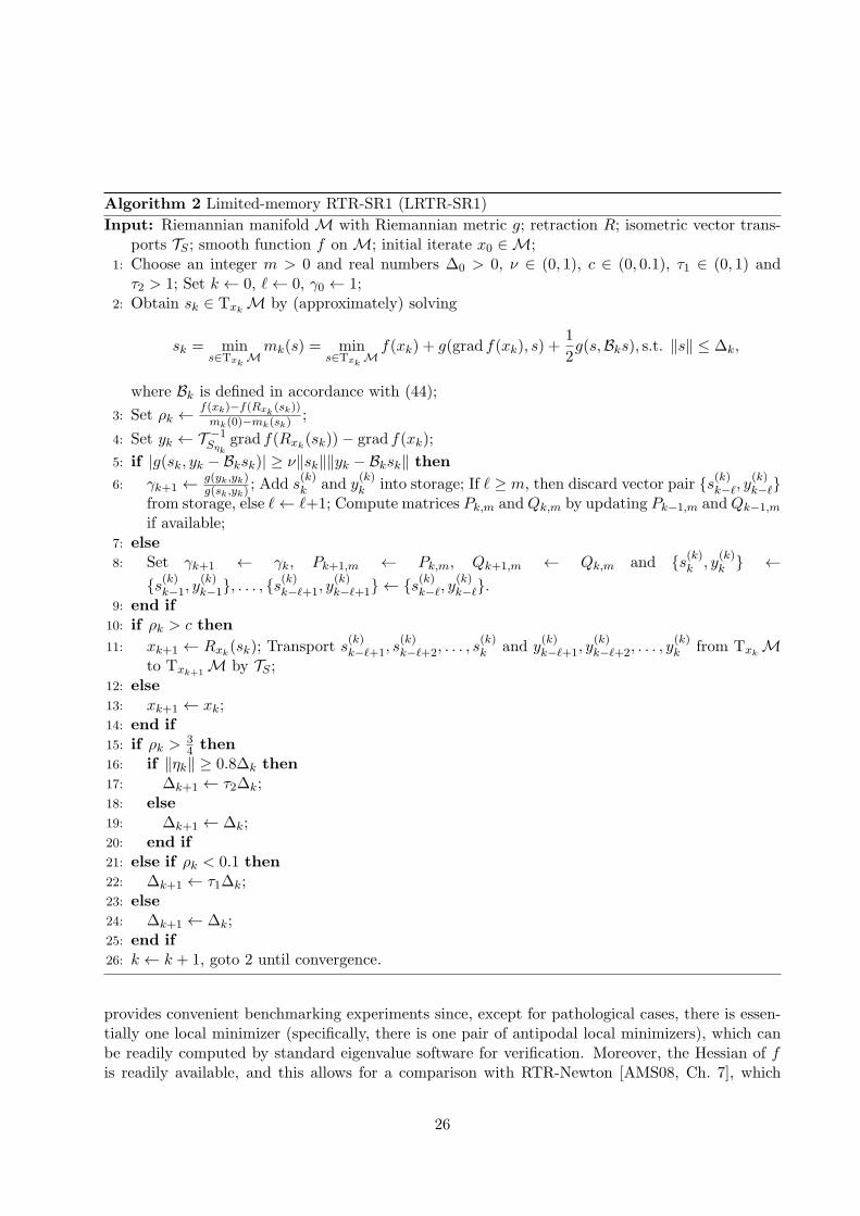
4 Limited memory version of RTR-SR1

In RTR-SR1 (Algorithm 1), storing Bk+1 = Tηk Bk+1 T −1ηkin matrix form may be inefficient for

two reasons. The first reason, which is also present in the Euclidean case, is that Bk+1 = Bk +(yk−Bksk)(yk−Bksk)

g(sk,yk−Bksk) is a rank-one modification of Bk. The second reason, specific to the Riemanniansetting, is that when M is a low-codimension submanifold of a Euclidean space E , it may bebeneficial to express Tηk as the restriction to Txk

M of a low-rank modification of the identity (6).Instead of storing full dense matrices, it may then be beneficial to store a few vectors that implicitlyrepresent them. This is the purpose of the limited memory version of RTR-SR1 presented in thissection.

24

The proposed limited memory RTR-SR1, called LRTR-SR1, is described in Algorithm 2. Itrelies on a Riemannian generalization of the compact representation of the classical (Euclidean)SR1 matrices presented in [BNS94, §5]. We set B0 = id. At step k > 0, we first choose a basicHessian approximation Bk0 , which in the Riemannian setting becomes a linear transformation ofTxkM. We advocate the choice

Bk0 = γk id,

where

γk =g(yk−1, yk−1)g(sk−1, yk−1)

,

which generalizes a choice usually made in the Euclidean case [NW06, (7.20)]. As in the Eu-clidean case, we let Sk,m and Yk,m contain the (at most) m most recent corrections, which in the

Riemannian setting must be transported to TxkM, yielding Sk,m = s(k)k−ℓ, s

(k)k−ℓ+1, . . . , s

(k)k−1 and

Yk,m = y(k)k−ℓ, y(k)k−ℓ+1, . . . , y

(k)k−1, where ℓ = minm, k and where s(k) denotes s transported to

TxkM. We then have the following Riemannian generalization of the limited-memory update

based on [BNS94, (5.2)]:

Bk = Bk0 + (Yk,m − Bk0Sk,m)(Pk,m − Sk,mBk0Sk,m)−1(Yk,m − Bk0Sk,m), k > 0,

where Pk,m = Dk,m+Lk,m+LTk,m, Dk,m = diagg(sk−ℓ, yk−ℓ), g(xk−ℓ+1, yk−ℓ+1), . . . , g(sk−1, yk−1),

and

(Lk,m)i,j =

g(sk−ℓ+i−1, yk−ℓ+j−1), if i > j;0, otherwise.

Moreover, letting Qk,m denote the matrix Sk,mSk,m, we obtain

Bk = γk id+(Yk,m − γkSk,m)(Pk,m − γkQk,m)−1(Yk,m − γkSk,m), k > 0. (44)

For all η ∈ TxkM, Bkη can thus be obtained from (44) using Yk,m, Sk,m, Pk,m and Qk,m. This

is how Bk is defined in Algorithm 2, except that the technicality that the B update may be skippedis also taken into account therein.

5 Numerical experiments

As an illustration, we investigate the performance of RTR-SR1 (Algorithm 1) and LRTR-SR1 (Algo-rithm 2) on a Rayleigh quotient minimization problem on the sphere and on a joint diagonalization(JD) problem on the Stiefel manifold.

For the Rayleigh quotient problem, the manifoldM is the sphere

Sn−1 = x ∈ R

n : xTx = 1

and the objective function f is defined by

f(x) = xTAx, (45)

where A is a given n by n symmetric matrix. Minimizing the Rayleigh quotient of A is equivalentto computing its leftmost eigenvector (see, e.g., [AMS08, §2.1.1]). The Rayleigh quotient problem

25

Algorithm 2 Limited-memory RTR-SR1 (LRTR-SR1)

Input: Riemannian manifoldM with Riemannian metric g; retraction R; isometric vector trans-ports TS ; smooth function f onM; initial iterate x0 ∈M;

1: Choose an integer m > 0 and real numbers ∆0 > 0, ν ∈ (0, 1), c ∈ (0, 0.1), τ1 ∈ (0, 1) andτ2 > 1; Set k ← 0, ℓ← 0, γ0 ← 1;

2: Obtain sk ∈ TxkM by (approximately) solving

sk = mins∈Txk

Mmk(s) = min

s∈TxkM

f(xk) + g(grad f(xk), s) +1

2g(s,Bks), s.t. ‖s‖ ≤ ∆k,

where Bk is defined in accordance with (44);

3: Set ρk ←f(xk)−f(Rxk

(sk))

mk(0)−mk(sk);

4: Set yk ← T −1Sηkgrad f(Rxk

(sk))− grad f(xk);

5: if |g(sk, yk − Bksk)| ≥ ν‖sk‖‖yk − Bksk‖ then6: γk+1 ← g(yk,yk)

g(sk,yk); Add s

(k)k and y

(k)k into storage; If ℓ ≥ m, then discard vector pair s(k)k−ℓ, y

(k)k−ℓ

from storage, else ℓ← ℓ+1; Compute matrices Pk,m andQk,m by updating Pk−1,m andQk−1,mif available;

7: else

8: Set γk+1 ← γk, Pk+1,m ← Pk,m, Qk+1,m ← Qk,m and s(k)k , y(k)k ←

s(k)k−1, y(k)k−1, . . . , s

(k)k−ℓ+1, y

(k)k−ℓ+1 ← s

(k)k−ℓ, y

(k)k−ℓ.

9: end if

10: if ρk > c then

11: xk+1 ← Rxk(sk); Transport s

(k)k−ℓ+1, s

(k)k−ℓ+2, . . . , s

(k)k and y

(k)k−ℓ+1, y

(k)k−ℓ+2, . . . , y

(k)k from Txk

Mto Txk+1

M by TS ;12: else

13: xk+1 ← xk;14: end if

15: if ρk > 34 then

16: if ‖ηk‖ ≥ 0.8∆k then

17: ∆k+1 ← τ2∆k;18: else

19: ∆k+1 ← ∆k;20: end if

21: else if ρk < 0.1 then

22: ∆k+1 ← τ1∆k;23: else

24: ∆k+1 ← ∆k;25: end if

26: k ← k + 1, goto 2 until convergence.

provides convenient benchmarking experiments since, except for pathological cases, there is essen-tially one local minimizer (specifically, there is one pair of antipodal local minimizers), which canbe readily computed by standard eigenvalue software for verification. Moreover, the Hessian of fis readily available, and this allows for a comparison with RTR-Newton [AMS08, Ch. 7], which

26

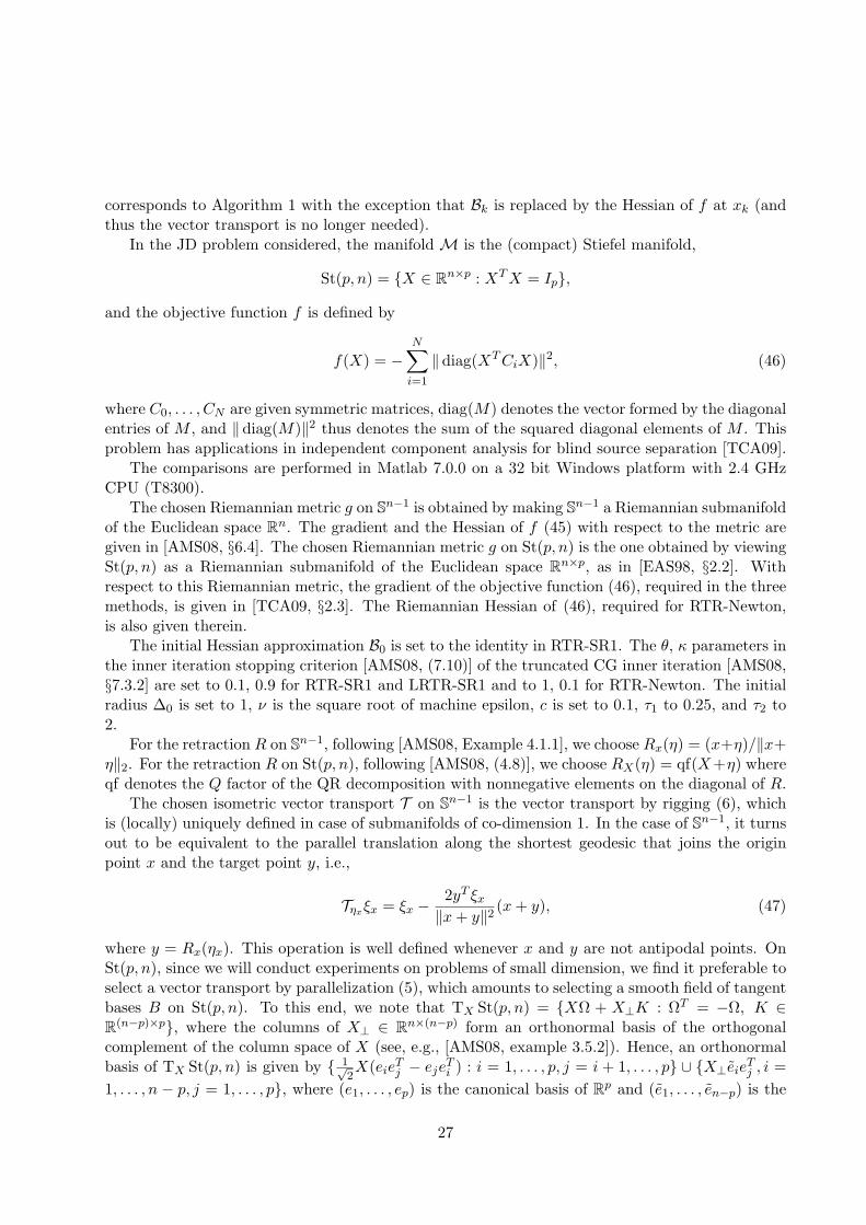
corresponds to Algorithm 1 with the exception that Bk is replaced by the Hessian of f at xk (andthus the vector transport is no longer needed).

In the JD problem considered, the manifoldM is the (compact) Stiefel manifold,

St(p, n) = X ∈ Rn×p : XTX = Ip,

and the objective function f is defined by

f(X) = −N∑

i=1

‖ diag(XTCiX)‖2, (46)

where C0, . . . , CN are given symmetric matrices, diag(M) denotes the vector formed by the diagonalentries of M , and ‖ diag(M)‖2 thus denotes the sum of the squared diagonal elements of M . Thisproblem has applications in independent component analysis for blind source separation [TCA09].

The comparisons are performed in Matlab 7.0.0 on a 32 bit Windows platform with 2.4 GHzCPU (T8300).

The chosen Riemannian metric g on Sn−1 is obtained by making Sn−1 a Riemannian submanifold

of the Euclidean space Rn. The gradient and the Hessian of f (45) with respect to the metric are

given in [AMS08, §6.4]. The chosen Riemannian metric g on St(p, n) is the one obtained by viewingSt(p, n) as a Riemannian submanifold of the Euclidean space R

n×p, as in [EAS98, §2.2]. Withrespect to this Riemannian metric, the gradient of the objective function (46), required in the threemethods, is given in [TCA09, §2.3]. The Riemannian Hessian of (46), required for RTR-Newton,is also given therein.

The initial Hessian approximation B0 is set to the identity in RTR-SR1. The θ, κ parameters inthe inner iteration stopping criterion [AMS08, (7.10)] of the truncated CG inner iteration [AMS08,§7.3.2] are set to 0.1, 0.9 for RTR-SR1 and LRTR-SR1 and to 1, 0.1 for RTR-Newton. The initialradius ∆0 is set to 1, ν is the square root of machine epsilon, c is set to 0.1, τ1 to 0.25, and τ2 to2.

For the retraction R on Sn−1, following [AMS08, Example 4.1.1], we choose Rx(η) = (x+η)/‖x+

η‖2. For the retraction R on St(p, n), following [AMS08, (4.8)], we choose RX(η) = qf(X+η) whereqf denotes the Q factor of the QR decomposition with nonnegative elements on the diagonal of R.

The chosen isometric vector transport T on Sn−1 is the vector transport by rigging (6), which

is (locally) uniquely defined in case of submanifolds of co-dimension 1. In the case of Sn−1, it turnsout to be equivalent to the parallel translation along the shortest geodesic that joins the originpoint x and the target point y, i.e.,

Tηxξx = ξx −2yT ξx‖x+ y‖2 (x+ y), (47)

where y = Rx(ηx). This operation is well defined whenever x and y are not antipodal points. OnSt(p, n), since we will conduct experiments on problems of small dimension, we find it preferable toselect a vector transport by parallelization (5), which amounts to selecting a smooth field of tangentbases B on St(p, n). To this end, we note that TX St(p, n) = XΩ + X⊥K : ΩT = −Ω, K ∈R(n−p)×p, where the columns of X⊥ ∈ R

n×(n−p) form an orthonormal basis of the orthogonalcomplement of the column space of X (see, e.g., [AMS08, example 3.5.2]). Hence, an orthonormalbasis of TX St(p, n) is given by 1√

2X(eie

Tj − eje

Ti ) : i = 1, . . . , p, j = i + 1, . . . , p ∪ X⊥eieTj , i =

1, . . . , n − p, j = 1, . . . , p, where (e1, . . . , ep) is the canonical basis of Rp and (e1, . . . , en−p) is the

27

canonical basis of Rn−p. To ensure that the obtained field of tangent bases is smooth, we need tochoose X⊥ as a smooth function of X. This can be done locally by extracting the n−p last columnsof the Gram-Schmidt orthonormalization of

[

X C]

where C is a given n × (n − p) matrix. Inpractice, we have observed that Matlab’s null function applied to X works adequately to producean X⊥.

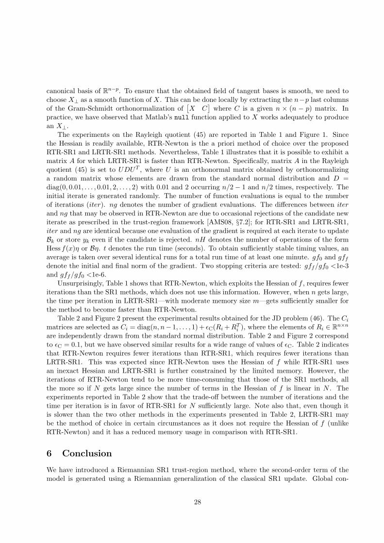
The experiments on the Rayleigh quotient (45) are reported in Table 1 and Figure 1. Sincethe Hessian is readily available, RTR-Newton is the a priori method of choice over the proposedRTR-SR1 and LRTR-SR1 methods. Nevertheless, Table 1 illustrates that it is possible to exhibit amatrix A for which LRTR-SR1 is faster than RTR-Newton. Specifically, matrix A in the Rayleighquotient (45) is set to UDUT , where U is an orthonormal matrix obtained by orthonormalizinga random matrix whose elements are drawn from the standard normal distribution and D =diag(0, 0.01, . . . , 0.01, 2, . . . , 2) with 0.01 and 2 occurring n/2− 1 and n/2 times, respectively. Theinitial iterate is generated randomly. The number of function evaluations is equal to the numberof iterations (iter). ng denotes the number of gradient evaluations. The differences between iterand ng that may be observed in RTR-Newton are due to occasional rejections of the candidate newiterate as prescribed in the trust-region framework [AMS08, §7.2]; for RTR-SR1 and LRTR-SR1,iter and ng are identical because one evaluation of the gradient is required at each iterate to updateBk or store yk even if the candidate is rejected. nH denotes the number of operations of the formHess f(x)η or Bη. t denotes the run time (seconds). To obtain sufficiently stable timing values, anaverage is taken over several identical runs for a total run time of at least one minute. gf0 and gffdenote the initial and final norm of the gradient. Two stopping criteria are tested: gff/gf0 <1e-3and gff/gf0 <1e-6.

Unsurprisingly, Table 1 shows that RTR-Newton, which exploits the Hessian of f , requires feweriterations than the SR1 methods, which does not use this information. However, when n gets large,the time per iteration in LRTR-SR1—with moderate memory size m—gets sufficiently smaller forthe method to become faster than RTR-Newton.

Table 2 and Figure 2 present the experimental results obtained for the JD problem (46). The Ci

matrices are selected as Ci = diag(n, n− 1, . . . , 1)+ ǫC(Ri +RTi ), where the elements of Ri ∈ R

n×n

are independently drawn from the standard normal distribution. Table 2 and Figure 2 correspondto ǫC = 0.1, but we have observed similar results for a wide range of values of ǫC. Table 2 indicatesthat RTR-Newton requires fewer iterations than RTR-SR1, which requires fewer iterations thanLRTR-SR1. This was expected since RTR-Newton uses the Hessian of f while RTR-SR1 usesan inexact Hessian and LRTR-SR1 is further constrained by the limited memory. However, theiterations of RTR-Newton tend to be more time-consuming that those of the SR1 methods, allthe more so if N gets large since the number of terms in the Hessian of f is linear in N . Theexperiments reported in Table 2 show that the trade-off between the number of iterations and thetime per iteration is in favor of RTR-SR1 for N sufficiently large. Note also that, even though itis slower than the two other methods in the experiments presented in Table 2, LRTR-SR1 maybe the method of choice in certain circumstances as it does not require the Hessian of f (unlikeRTR-Newton) and it has a reduced memory usage in comparison with RTR-SR1.

6 Conclusion

We have introduced a Riemannian SR1 trust-region method, where the second-order term of themodel is generated using a Riemannian generalization of the classical SR1 update. Global con-

28

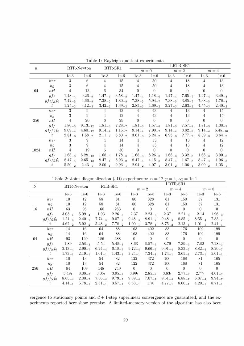
Table 1: Rayleigh quotient experiments

n RTR-Newton RTR-SR1LRTR-SR1

m = 0 m = 2 m = 41e-3 1e-6 1e-3 1e-6 1e-3 1e-6 1e-3 1e-6 1e-3 1e-6

64

iter 3 6 4 15 4 50 4 18 4 13ng 3 6 4 15 4 50 4 18 4 13nH 4 13 6 34 0 0 0 0 0 0gff 1.48

−4 9.26−9 1.47

−4 3.58−8 1.47

−4 1.18−6 1.47

−4 7.65−7 1.47

−4 3.49−8

gff/gf0 7.42−5 4.66

−9 7.38−5 1.80

−8 7.38−5 5.94

−7 7.38−5 3.85

−7 7.38−5 1.76

−8

t 1.25−3 3.12

−3 3.42−3 1.39

−2 2.85−3 4.69

−2 3.27−3 2.63

−2 4.55−3 2.40

−2

256

iter 3 9 4 13 4 43 4 13 4 15ng 3 9 4 13 4 43 4 13 4 15nH 4 20 6 29 0 0 0 0 0 0gff 1.80

−3 9.13−12 1.81

−3 2.28−7 1.81

−3 1.57−6 1.81

−3 7.57−8 1.81

−3 1.08−9

gff/gf0 9.09−4 4.60

−12 9.14−4 1.15

−7 9.14−4 7.90

−7 9.14−4 3.82

−8 9.14−4 5.45

−10

t 2.81−3 1.58

−2 2.11−2 6.80

−2 3.61−3 5.24

−2 6.93−3 2.77

−2 8.39−3 3.64

−2

1024

iter 3 9 4 14 4 53 4 13 4 12ng 3 9 4 14 4 53 4 13 4 12nH 4 19 6 30 0 0 0 0 0 0gff 1.68

−3 5.28−12 1.68

−3 1.78−8 1.68

−3 8.26−8 1.68

−3 3.32−8 1.68

−3 3.90−8

gff/gf0 8.47−4 2.65

−12 8.47−4 8.93

−9 8.47−4 4.15

−8 8.47−4 1.67

−8 8.47−4 1.96

−8

t 5.50−2 2.43

−1 2.00−1 9.96

−1 2.94−2 4.07

−1 3.01−2 1.06

−1 3.09−2 1.05

−1

Table 2: Joint diagonalization (JD) experiments: n = 12, p = 4, ǫC = 1e-1

N RTR-Newton RTR-SR1LRTR-SR1

m = 2 m = 4 m = 81e-3 1e-6 1e-3 1e-6 1e-3 1e-6 1e-3 1e-6 1e-3 1e-6

16

iter 10 12 58 81 80 328 61 150 57 131ng 10 12 58 81 80 328 61 150 57 131nH 63 96 160 253 0 0 0 0 0 0gff 3.03

−1 5.99−4 1.93 2.26

−3 2.37 2.23−3 2.37 2.21

−3 2.14 1.96−3

gff/gf0 1.21−4 2.40

−7 7.74−4 9.07

−7 9.48−4 8.91

−7 9.48−4 8.85

−7 8.55−4 7.83

−7

t 4.62−2 5.92

−2 5.48−2 7.78

−2 1.00−1 3.78

−1 8.75−2 2.13

−1 1.01−1 2.41

−1

64

iter 14 16 64 88 163 402 83 176 109 199ng 14 16 64 88 163 402 83 176 109 199nH 93 120 186 288 0 0 0 0 0 0gff 1.89 2.58

−3 5.54 5.48−3 8.63 8.57

−3 8.79 7.39−3 7.82 7.28

−3

gff/gf0 2.13−4 2.90

−7 6.24−4 6.18

−7 9.72−4 9.66

−7 9.91−4 8.33

−7 8.82−4 8.20

−7

t 1.73−1 2.19

−1 1.01−1 1.43

−1 3.24−1 7.34

−1 1.74−1 3.65

−1 2.73−1 5.01

−1

256

iter 10 13 54 82 122 372 100 168 81 165ng 10 13 54 82 122 372 100 168 81 165nH 64 109 148 240 0 0 0 0 0 0gff 3.491 8.08

−3 3.051 3.95−2 3.991 2.85

−2 3.831 2.77−2 2.771 4.01

−2

gff/gf0 8.65−4 2.00

−7 7.56−4 9.79

−7 9.89−4 7.07

−7 9.51−4 6.88

−7 6.87−4 9.94

−7

t 4.14−1 6.78

−1 2.31−1 3.57

−1 6.83−1 1.70 4.77

−1 8.06−1 4.20

−1 8.71−1

vergence to stationary points and d + 1-step superlinear convergence are guaranteed, and the ex-periments reported here show promise. A limited-memory version of the algorithm has also been

29

0 0.2 0.4 0.6 0.8 1 1.2 1.410

−15

10−10

10−5

100

105

time(second)

|gra

d f|

comparison of algorithms, n:1024

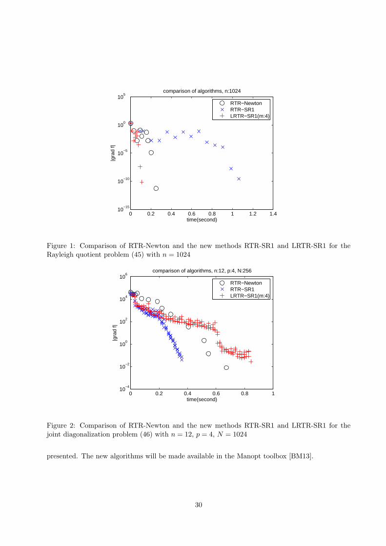
RTR−NewtonRTR−SR1LRTR−SR1(m:4)

Figure 1: Comparison of RTR-Newton and the new methods RTR-SR1 and LRTR-SR1 for theRayleigh quotient problem (45) with n = 1024

0 0.2 0.4 0.6 0.8 110

−4

10−2

100

102

104

106

time(second)

|gra

d f|

comparison of algorithms, n:12, p:4, N:256

RTR−NewtonRTR−SR1LRTR−SR1(m:4)

Figure 2: Comparison of RTR-Newton and the new methods RTR-SR1 and LRTR-SR1 for thejoint diagonalization problem (46) with n = 12, p = 4, N = 1024

presented. The new algorithms will be made available in the Manopt toolbox [BM13].

30

References

[ABG07] P.-A. Absil, C. G. Baker, and K. A. Gallivan. Trust-region methods on Riemannianmanifolds. Found. Comput. Math., 7(3):303–330, July 2007.

[ADM+02] Roy L. Adler, Jean-Pierre Dedieu, Joseph Y. Margulies, Marco Martens, and MikeShub. Newton’s method on Riemannian manifolds and a geometric model for thehuman spine. IMA J. Numer. Anal., 22(3):359–390, July 2002.

[AM12] P.-A. Absil and Jerome Malick. Projection-like retractions on matrix manifolds. SIAMJ. Optim., 22(1):135–158, 2012.

[AMS08] P.-A. Absil, R. Mahony, and R. Sepulchre. Optimization Algorithms on Matrix Mani-folds. Princeton University Press, Princeton, NJ, 2008.

[ATV11] Bijan Afsari, Roberto Tron, and Rene Vidal. On the convergence of gradient descentfor finding the Riemannian center of mass, 2011. arXiv:1201.0925v1.

[BA11] N. Boumal and P.-A. Absil. RTRMC: A Riemannian trust-region method for low-rank matrix completion. In J. Shawe-Taylor, R.S. Zemel, P. Bartlett, F.C.N. Pereira,and K.Q. Weinberger, editors, Advances in Neural Information Processing Systems 24(NIPS), pages 406–414. 2011.

[BKS96] Richard H. Byrd, Humaid Fayez Khalfan, and Robert B. Schnabel. Analysis of asymmetric rank-one trust region method. SIAM J. Optim., 6(4):1025–1039, November1996.

[BM13] Nicolas Boumal and Bamdev Mishra. The Manopt toolbox. http://www.manopt.org,2013. version 1.0.1.

[BNS94] Richard H. Byrd, Jorge Nocedal, and Robert B. Schnabel. Representations of quasi-Newton matrices and their use in limited memory methods. Math. Program., 63(2):129–156, January 1994.

[Boo03] William M. Boothby. An Introduction to Differentiable Manifolds and RiemannianGeometry. Academic Press, 2003. Revised Second Edition.

[Bor12] Ruediger Borsdorf. Structured Matrix Nearness Problems: Theory and Algorithms.PhD thesis, School of Mathematics, The University of Manchester, 2012. MIMS Eprint2012.63.

[CGT91] A. R. Conn, N. I. M. Gould, and Ph. L. Toint. Convergence of quasi-Newton matricesgenerated by the symmetric rank one update. Math. Program., 50:177–195, 1991.

[CGT00] Andrew R. Conn, Nicholas I. M. Gould, and Philippe L. Toint. Trust-Region Methods.MPS/SIAM Series on Optimization. Society for Industrial and Applied Mathematics(SIAM), Philadelphia, PA, 2000.

[Cha06] Isaac Chavel. Riemannian geometry, volume 98 of Cambridge Studies in AdvancedMathematics. Cambridge University Press, Cambridge, second edition, 2006.

31

[dC92] M. P. do Carmo. Riemannian geometry. Mathematics: Theory & Applications, 1992.

[EAS98] Alan Edelman, Tomas A. Arias, and Steven T. Smith. The geometry of algorithmswith orthogonality constrains. SIAM J. Matrix Anal. Appl., 20(2):303–353, 1998.

[GQA12] Kyle A. Gallivan, Chunhong Qi, and P.-A. Absil. A Riemannian Dennis–More condi-tion. In Michael W. Berry, Kyle A. Gallivan, Efstratios Gallopoulos, Ananth Grama,Bernard Philippe, Yousef Saad, and Faisal Saied, editors, High-Performance ScientificComputing, pages 281–293. Springer London, 2012.

[IAVD11] Mariya Ishteva, P.-A. Absil, Sabine Van Huffel, and Lieven De Lathauwer. Best lowmultilinear rank approximation of higher-order tensors, based on the Riemannian trust-region scheme. SIAM J. Matrix Anal. Appl., 32(1):115–135, 2011.

[JBAS10] M. Journee, F. Bach, P.-A. Absil, and R. Sepulchre. Low-rank optimization on the coneof positive semidefinite matrices. SIAM J. Optim., 20(5):2327–2351, 2010.

[JD13] Bo Jiang and Yu-Hong Dai. A framework of constraint preserving update schemes foroptimization on Stiefel manifold, 2013. arXiv:1301.0172.

[KBS93] H. Fayez Khalfan, R. H. Byrd, and R. B. Schnabel. A theoretical and experimentalstudy of the symmetric rank-one update. SIAM J. Optim., 3(1):1–24, 1993.

[KS12] M. Kleinsteuber and H. Shen. Blind source separation with compressively sensed linearmixtures. IEEE Signal Processing Letters, 19(2):107–110, 2012.

[MMBS11] B. Mishra, G. Meyer, F. Bach, and R. Sepulchre. Low-rank optimization with tracenorm penalty, 2011. arXiv:1112.2318v1.

[NW06] Jorge Nocedal and Stephen J. Wright. Numerical optimization. Springer Series inOperations Research and Financial Engineering. Springer, New York, second edition,2006.

[O’N83] Barrett O’Neill. Semi-Riemannian Geometry, volume 103 of Pure and Applied Mathe-matics. Academic Press Inc. [Harcourt Brace Jovanovich Publishers], New York, 1983.

[RW12] Wolfgang Ring and Benedikt Wirth. Optimization methods on Riemannian manifoldsand their application to shape space. SIAM J. Optim., 22(2):596–627, 2012.

[SAG+12] S. E. Selvan, U. Amato, K. A. Gallivan, C. Qi, M. F. Carfora, M. Larobina, and B. Al-fano. Descent algorithms on oblique manifold for source-adaptive ICA contrast. NeuralNetworks and Learning Systems, IEEE Transactions on, 23(12):1930–1947, 2012.

[SI13] Hiroyuki Sato and Toshihiro Iwai. Convergence analysis for the riemannian conjugategradient method, 2013. arXiv:1302.0125.

[SL10] B. Savas and L.-H. Lim. Quasi-Newton methods on Grassmannians and multilinearapproximations of tensors. SIAM J. Sci. Comput., 32(6):3352–3393, 2010.

[Sti35] E. Stiefel. Richtungsfelder und Fernparallelismus in n-dimensionalen Mannig-faltigkeiten. Comment. Math. Helv., 8(1):305–353, 1935.

32

[TCA09] Fabian J. Theis, Thomas P. Cason, and P.-A. Absil. Soft dimension reduction for ICAby joint diagonalization on the Stiefel manifold. In Proc. ICA 2009, volume 5441 ofLNCS, pages 354–361, Paraty, Brazil, 2009. Springer.

[TVSC11] P. Turaga, A. Veeraraghavan, A. Srivastava, and R. Chellappa. Statistical computationson Grassmann and Stiefel manifolds for image and video-based recognition. PatternAnalysis and Machine Intelligence, IEEE Transactions on, 33(11):2273–2286, 2011.

[VV10] Bart Vandereycken and Stefan Vandewalle. A Riemannian optimization approach forcomputing low-rank solutions of Lyapunov equations. SIAM J. Matrix Anal. Appl.,31(5):2553–2579, 2010.

[WY12] Zaiwen Wen and Wotao Yin. A feasible method for optimization with orthogonalityconstraints. Math. Program., pages 1–38, 2012.

33