A Riemannian Conjugate Gradient Algorithm with Implicit Vector

Transport for Optimization on the Stiefel Manifold

H. Oviedoa and H. Larab

aMathematics Research Center, CIMAT A.C. Guanajuato, Mexico; bUniversidade Federal deSanta Catarina. Campus Blumenau. Brazil

ARTICLE HISTORY

Compiled February 24, 2018

ABSTRACTIn this paper, a reliable curvilinear search algorithm for solving optimization prob-lems over the Stiefel manifold is presented. This method is inspired by the conjugategradient method, with the purpose of obtain a new direction search that guaranteesdescent of the objective function in each iteration. The merit of this algorithm liesin the fact that is not necessary extra calculations associated to vector transport.To guarantee the feasibility of each iteration, a retraction based on the QR factor-ization is considered. In addition, this algorithm enjoys global convergence. Finally,two numerical experiments are given to confirm the effectiveness and efficiency ofpresented method with respect to some other state of the art algorithms.

KEYWORDSoptimization on manifolds, Stiefel manifold, conjugate gradient method, vectortransport.

AMS CLASSIFICATION49K99; 49Q99; 49M30; 49M37; 90C30; 68W01

1. Introduction

In this paper, we consider the following manifold-constrained optimization problem

minF(X) s.t. X ∈ St(n, p), (1)

where F : Rn×p → R is a continuously differentiable real-valued function andSt(n, p) = X ∈ Rn×p : X>X = I is known as Stiefel manifold, where I denote theidentity matrix.

Nowadays, manifold-constrained optimization is an active area of research due tothe wide range of applications that this involves, for example, in machine learning[1], recommendation systems (matrix completion problem) [2–4], electronic structure[5], joint diagonalization [6], multi-view clustering [7], maxcut problems [8]. Forthe specific case of the Stiefel manifold, the problem (1) arises in applications

Harry Fernando Oviedo Leon. Email: harry.oviedo@cimat.mx

Hugo Jose Lara Urdaneta. Email: hugo.lara.urdaneta@ufsc.br

such as, 1-bit compressed sensing [9], linear and nonlinear eigenvalue problems[5,10,11], orthogonal procrustes problems and weighted orthogonal procrustes [12–14],image segmentation [15], sensor localization [16], manifold learning [17], p-harmonicflow [18], among others. In addition, many techniques for reducing the dimensional-ity of data in the area of pattern recognition can be formulated as the problem (1) [19].

It have been developed works that address the general optimization problem onRiemannian manifold since the decade of the 70’s [20]. However, the first purposealgorithms specially designed to deal with the problem (1) appeared in the 1990’s,[21–23]. These seminal works exploit the geometry of the feasible set St(n, p), andthe underlined algorithms perform a serie of descent steps along a geodesic (the curveof shortest length between two points on a manifold). Such search is intractablein practice. In 2002, Manton [24] presents two algorithms that break with theparadigm of descending along a geodesic. Since that date, it has emerged differentpragmatic algorithms that approximate descent search along other smooth curves onthe manifold. These curves are defined by mappings that convert any displacementin the tangent space to a point on the manifold, these smooth mappings are calledretractions. Some gradient-type methods based on retractions to solve the problem (1)have been proposed in [25–30]. Other first-order algorithms such as the Riemannianconjugate gradient method (RCG) and Quasi-Newton method are the subject in[23,27,31–33]. Furthermore some Newton‘s type algorithms, which use second-orderinformation, appear in [23,27,34].

All the conjugated gradients algorithms introduced in [23,27,31,32] need to usesome “vector transport” (the definition of this concept is in section 2), which entails agreater computational effort associated to a projection onto the manifold. This paperintroduces a new RCG algorithm based on retraction that avoids extra calculationsrelated to vector transport, which emerge implicitly from the previous computations.

In this article, an efficient monotone algorithm of linear search on manifold isproposed, which is inspired by the standard conjugate gradient method, in order toobtain a novel version of the Riemannian Conjugate Gradient Method that does notrequire to use any vector transport or parallel transport explicitly. In this way, wedesigned a feasible Conjugated Gradient Method to address the problem (1) and wealso provide a new vector transport for the Stiefel manifold. This algorithm preservethe feasibility of each iterate by using QR re-orthogonalization procedure. Therefore,we get a descent algorithm SVD-free and also free of matrix inversion, unlike manyother methods of the state of the art.

The remainder of this paper is organized as follows. In the next section, we introducesome notations and definitions about Riemannian geometry, which may not be familiarto some readers, furthermore, in subsection 2.1 we provide a self-contained introductionto geometry of the Stiefel manifold and we introduce a new vector transport for theStiefel manifold. In section 3, we review the Riemannian conjugate gradient methods,which are described in [21,27]. In section 4, we describe a new feasible update schemeto address the problem (1) and propose our algorithm. Section 5 is dedicated to presentsome numerical results. Finally, the conclusions and discussions are commented in thelast section.

2

2. Notation and background

In the remainder of this work, we will use the following concepts and notations.Let A be a n-by-n matrix with real entries. We say that A is skew-symmetricif A> = −A. The trace of A, denoted by Tr[A], is defined as the sum of thediagonal entries. The Euclidean inner product of two matrices A,B ∈ Rm×n isdefined as 〈A,B〉e :=

∑i,j aijbij = Tr[A>B], where aij and bij denote the elements

(i, j) of the matrices A and B respectively. Furthermore, the canonical inner prod-uct associated with a matrix X ∈ Rm×n is defined as 〈A,B〉c := Tr[A>(I− 1

2XX>)B].

The Frobenius norm is defined as the metric induced by the Euclidean inner product,that is, ||A||F =

√〈A,A〉e. Let F : Rn×p → R be a differentiable function, and denote

by G := DF(X) :=(∂F(X)∂xij

)the matrix of partial derivatives of F with respect to X

(that is, the Euclidean gradient of F). The directional derivative of F along a givenmatrix Z ∈ Rn×p at a given point X is defined by

DF(X)[Z] := limt→0

F(X + tZ)−F(X)

t= 〈G,Z〉e.

A Riemannian manifold M is a manifold whose tangent spaces TxM at a givenx ∈ M are endowed with a smooth local inner product g(ηx, ξx) = 〈ηx, ξx〉x, whereηx, ξx ∈ TxM. This smoothly varying inner product is called the Riemannian metric.Let f : M → R be a differentiable scalar field on a Riemannian manifold M. TheRiemannian gradient of f at x, denoted by gradf(x), is defined as the unique elementof TxM that satisfies

〈gradf(x), ξ〉x = Df(X)[ξ], ∀ξ ∈ TxM.

Now, let f : E → R be a differentiable objective function that we want to minimizeon a Riemannian submanifold M of a Euclidean space E , and let ∇f(x) be the Eu-clidean gradient of f at x ∈ E . Then the Riemannian gradient of f at x ∈M is equalto the orthogonal projection of the Euclidean gradient ∇f(x) onto TxM, that is

gradf(x) = PTxM[∇f(x)],

where PTxM[·] denote the orthogonal projection onto TxM.

Other concepts of interest are retraction and vector transport. A retraction is asmooth mapping that transforms any displacement in the tangent space to a pointon the manifold that satisfies some technical conditions. Below we present a rigorousdefinition of a retraction.

Definition 2.1 (Definition 4.1.1 in [27]). A retraction on a manifold M is a smoothmapping R from the tangent bundle TM :=

⋃x∈M TxM onto M with the following

properties. Let Rx denote the restriction of R to TxM.

(1) Rx(0x) = x, where 0x denotes the zero element of TxM

3

(2) With the canonical identification, T0xTxM' TxM, Rx satisfies

DRx(0x) = idTxM,

where idTxM denotes the identity mapping on TxM.

This concept is widely used in optimization methods on manifold, both thoseof the first order (Line Search Methods, Steepest Descent, Conjugated Gradient,Quasi-Newton, among others) as well as those of second order (for example Newtonmethod). The choice of an appropriate retraction when designing an optimizationmethod is essential to obtain an efficient algorithm.

When developing algorithms on manifolds based on retractions, operations involvingvectors in different tangent spaces can appear. To overcome this technical difficulty, theconcept of vector transport have been used. This concept is fundamental to establishthe Riemannian Conjugate Gradient methods.

Definition 2.2 (Definition 8.1.1 in [27]). A vector transport T on a manifoldM is asmooth mapping

TM⊕ TM→ TM : (η, ξ) 7→ Tη(ξ) ∈ TM,

satisfying the following properties for all x ∈ M where ⊕ denote the Whitney sum,that is,

TM⊕ TM = (η, ξ) : η, ξ ∈ TxM, x ∈M.

(1) There exists a retraction R, called the retraction associated with T , such that

π(Tη(ξ)) = Rx(η), η, ξ ∈ TxM,

where π(Tη(ξ)) denotes the foot of the tangent vector Tη(ξ).(2) T0x

(ξ) = ξ for all ξ ∈ TxM.(3) Tη(aξ + bζ) = aTη(ξ) + bTη(ζ), for all a, b ∈ R and η, ξ, ζ ∈ TxM.

2.1. The geometry of the Stiefel manifold and the gradient of theobjective function

In this subsection, we review the geometry of the Stiefel manifold St(n, p), asdiscussed in [23,27].

It is well known that the Stiefel manifold St(n, p) is an embedded submanifold ofRn×p. The tangent space of St(n, p) at X ∈ St(n, p) is

TXSt(n, p) = Z ∈ Rn×p : Z>X +X>Z = 0.

The following proposition provides us with an alternative characterization ofTXSt(n, p)

4

Proposition 2.3. Let X be a matrix in St(n, p) and ΩX the set defined by,

ΩX = Z ∈ Rn×p : Z = WX, for some skew-symmetric matrix W ∈ Rp×p.

Then TXSt(n, p) = ΩX .

Proof. Let Z ∈ TXSt(n, p) be an arbitrary matrix, and define by WZ = PXZX> −

XZ>PX , where PX = I− 12XX

>. Clearly, WZ is a skew-symmetric matrix. Using the

fact that Z>X = −X>Z and X ∈ St(n, p) we have,

WZX = PXZ −XZ>PXX

= Z − 1

2XX>Z − 1

2XZ>X

= Z,

therefore, we conclude that TXSt(n, p) ⊂ ΩX .

On the other hand, consider Z ∈ ΩX , then there exists an skew-symmetric matrixW ∈ Rn×n such that Z = WX. So, note that,

Z>X +X>Z = (WX)>X +X>WX = −X>WX +X>WX = 0,

thus, we have that ΩX ⊂ TXSt(n, p), which completes the proof.

If we endorse the Stiefel manifold with the Riemannian metric 〈·, ·〉e inherited fromthe embedding space Rn×p, then the normal space to TXSt(n, p) is

(TXSt(n, p))⊥ = XS : S> = S, S ∈ Rp×p.

The orthogonal projection onto TXSt(n, p) is

PTXSt(n,p)[ξ] = (I −XX>)ξ +Xskew(X>ξ), (2)

where skew(W ) := 12(W −W>) denote the skew-symmetric part of the square matrix

W . The Riemannian gradient of objective function F of the equation (1) at X underthe Euclidean inner product 〈·, ·〉e is

∇eF(X) := gradF(X) = PTXSt(n,p)[G] = (I −XX>)G+Xskew(X>G),

where G is the Euclidean gradient of F at X. And the Riemannian gradient of F atX under canonical inner product 〈·, ·〉c is

∇cF(X) := G−XG>X,

for more details about this two Riemannian gradient see [25,27]. Observe that ∇cF(X)can be rewritten as

5

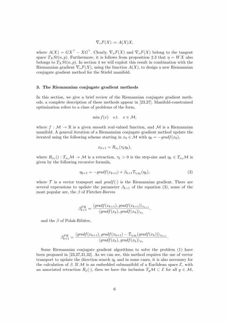
∇cF(X) := A(X)X,

where A(X) = GX> − XG>. Clearly, ∇eF(X) and ∇cF(X) belong to the tangentspace TXSt(n, p). Furthermore, it is follows from proposition 2.3 that η = WX alsobelongs to TXSt(n, p). In section 4 we will exploit this result in combination with theRiemannian gradient ∇cF(X), using the function A(X), to design a new Riemannianconjugate gradient method for the Stiefel manifold.

3. The Riemannian conjugate gradient methods

In this section, we give a brief review of the Riemannian conjugate gradient meth-ods, a complete description of these methods appear in [23,27]. Manifold-constrainedoptimization refers to a class of problems of the form,

min f(x) s.t. x ∈M,

where f : M → R is a given smooth real-valued function, and M is a Riemannianmanifold. A general iteration of a Riemannian conjugate gradient method update theiterated using the following scheme starting in x0 ∈M with η0 = −gradf(x0),

xk+1 = Rxk(τkηk),

where Rxk() : Txk

M → M is a retraction, τk > 0 is the step-size and ηk ∈ TxkM is

given by the following recursive formula,

ηk+1 = −gradf(xk+1) + βk+1Tτkηk(ηk), (3)

where T is a vector transport and gradf(·) is the Riemannian gradient. There areseveral expressions to update the parameter βk+1 of the equation (3), some of themost popular are, the β of Fletcher-Reeves

βFRk+1 =〈gradf(xk+1), gradf(xk+1)〉xk+1

〈gradf(xk), gradf(xk)〉xk

,

and the β of Polak-Ribiere,

βPRk+1 =〈gradf(xk+1), gradf(xk+1)− Tτkηk(gradf(xk))〉xk+1

〈gradf(xk), gradf(xk)〉xk

.

Some Riemannian conjugate gradient algorithms to solve the problem (1) havebeen proposed in [23,27,31,32]. As we can see, this method requires the use of vectortransport to update the direction search ηk and in some cases, it is also necessary forthe calculation of β. If M is an embedded submanifold of a Euclidean space E , withan associated retraction Rx(·), then we have the inclusion TyM ⊂ E for all y ∈ M,

6

and so, we can define the vector transport by

Tηx(ξx) = PRx(ηx)(ξx),

where Px denotes the orthogonal projector onto TxM. For the case when M is theStiefel manifold, this vector transport uses the orthogonal projector defined in (2),and makes the Riemannian conjugate gradient algorithm perform more matrix multi-plications per iteration than the Riemannian steepest descent. In [32], Zhu introducetwo novel vector transports associated with the Cayley transform retraction for Stiefel-constrained optimization. However its two vector transports require to invert a matrix,which can be computationally expensive. In the next section, we present a novel Rie-mannian conjugate gradient algorithm, which does not require to calculate a vectortransport.

4. A novel Riemannian Conjugate Gradient Algorithm

In this section, we formulate a concrete algorithm to address optimization problemson the Stiefel manifold with general objective functions. Specifically, we introducean update formula that preserves the restrictions using a retraction map based onQR re-orthogonalization. The proposal consists of a novel Riemannian ConjugateGradient Method (RCG), which does not need to use parallel transport or vectortransport explicitly, to update the direction search. This novelty is what differentiatesour proposal from the standard RCG algorithm discussed in section 3.

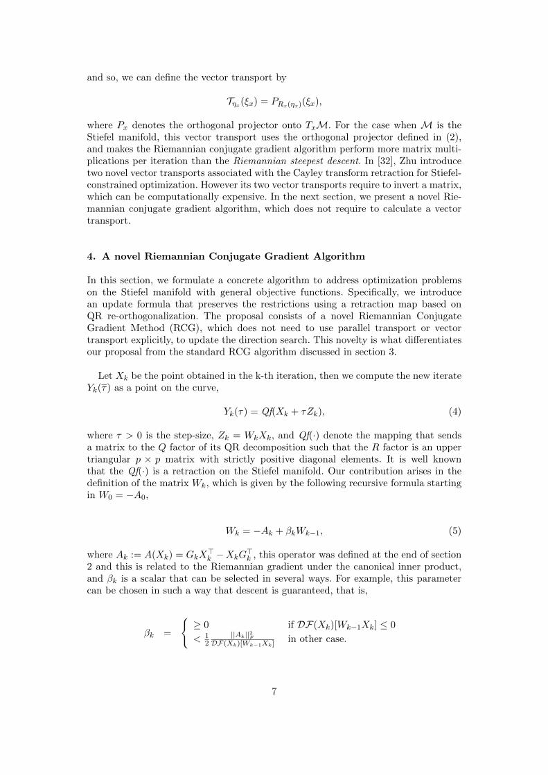
Let Xk be the point obtained in the k-th iteration, then we compute the new iterateYk(τ) as a point on the curve,

Yk(τ) = Qf(Xk + τZk), (4)

where τ > 0 is the step-size, Zk = WkXk, and Qf(·) denote the mapping that sendsa matrix to the Q factor of its QR decomposition such that the R factor is an uppertriangular p × p matrix with strictly positive diagonal elements. It is well knownthat the Qf(·) is a retraction on the Stiefel manifold. Our contribution arises in thedefinition of the matrix Wk, which is given by the following recursive formula startingin W0 = −A0,

Wk = −Ak + βkWk−1, (5)

where Ak := A(Xk) = GkX>k −XkG

>k , this operator was defined at the end of section

2 and this is related to the Riemannian gradient under the canonical inner product,and βk is a scalar that can be selected in several ways. For example, this parametercan be chosen in such a way that descent is guaranteed, that is,

βk =

≥ 0 if DF(Xk)[Wk−1Xk] ≤ 0

< 12

||Ak||2FDF(Xk)[Wk−1Xk] in other case.

7

However, in this paper we will use the parameters βk given by the well-known formulasof Fletcher-Reeves and Polak-Ribiere [35],

βFRk =||Ak||2F||Ak−1||2F

and βPRk =Tr[A>k (Ak −Ak−1)]

||Ak−1||2F.

In particular, we adopt a hybrid strategy, which is very used in the case of non-linearunconstrained optimization, that updates βk as follow,

βFR−PRk =

−βFRk if βPRk < −βFRk

βPRk if |βPRk | < βFRkβFRk if βPRk > βFRk ,

which has performed well on some applications.

Now, observe that Wk is an skew-symmetric matrix because this matrix is obtainedas the sum of two skew-symmetric matrices. This result implies that the proposeddirection search Zk = WkXk belongs to the tangent space of the Stiefel manifold atXk. On the other hand, by taking the inner product of Zk with the gradient matrixGk, using (5) and trace properties, we obtain

DF(Xk)[Zk] = Tr[G>kWkXk]

= −Tr[G>k AkXk] + βkTr[G>kWk−1Xk]

= −1

2||Ak||2F + βkTr[G

>kWk−1Xk]. (6)

Then we have from (6) that Zk may not be to descent direction at Xk, becausethe second term in (6) may dominate the first term and in this case, we obtainDF(Xk)[Zk] > 0. Nevertheless, this issue can be solved by resetting the directionsearch, that is, selecting βk as follows,

βk =

βFR−PRk if DF(Xk)[Zk] < 00 in other case.

(7)

Therefore, with this selection of the parameter βk we obtain an line search methodon matrix manifold that uses a search direction that satisfies the descent conditionand that is also in the tangent space of the manifold.

Now we introduce a new vector transport for the Stiefel manifold. Consider X ∈St(n, p), and ξX , ηX ,∈ TXSt(n, p), since ΩX = TXSt(n, p), then there exists skew-

symmetric matrices W, W ∈ Rn×n such that, ξX = WX and ηX = WX. Given aretraction RX(·) on the Stiefel manifold, we define our vector transport as,

TηX (ξX) := WRX(ηX). (8)

8

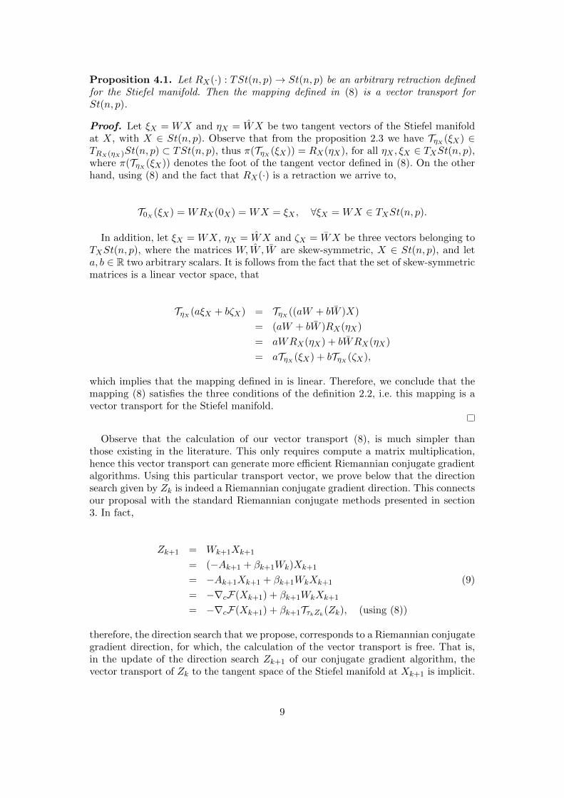
Proposition 4.1. Let RX(·) : TSt(n, p)→ St(n, p) be an arbitrary retraction definedfor the Stiefel manifold. Then the mapping defined in (8) is a vector transport forSt(n, p).

Proof. Let ξX = WX and ηX = WX be two tangent vectors of the Stiefel manifoldat X, with X ∈ St(n, p). Observe that from the proposition 2.3 we have TηX (ξX) ∈TRX(ηX)St(n, p) ⊂ TSt(n, p), thus π(TηX (ξX)) = RX(ηX), for all ηX , ξX ∈ TXSt(n, p),where π(TηX (ξX)) denotes the foot of the tangent vector defined in (8). On the otherhand, using (8) and the fact that RX(·) is a retraction we arrive to,

T0X(ξX) = WRX(0X) = WX = ξX , ∀ξX = WX ∈ TXSt(n, p).

In addition, let ξX = WX, ηX = WX and ζX = WX be three vectors belonging toTXSt(n, p), where the matrices W, W , W are skew-symmetric, X ∈ St(n, p), and leta, b ∈ R two arbitrary scalars. It is follows from the fact that the set of skew-symmetricmatrices is a linear vector space, that

TηX (aξX + bζX) = TηX ((aW + bW )X)

= (aW + bW )RX(ηX)

= aWRX(ηX) + bWRX(ηX)

= aTηX (ξX) + bTηX (ζX),

which implies that the mapping defined in is linear. Therefore, we conclude that themapping (8) satisfies the three conditions of the definition 2.2, i.e. this mapping is avector transport for the Stiefel manifold.

Observe that the calculation of our vector transport (8), is much simpler thanthose existing in the literature. This only requires compute a matrix multiplication,hence this vector transport can generate more efficient Riemannian conjugate gradientalgorithms. Using this particular transport vector, we prove below that the directionsearch given by Zk is indeed a Riemannian conjugate gradient direction. This connectsour proposal with the standard Riemannian conjugate methods presented in section3. In fact,

Zk+1 = Wk+1Xk+1

= (−Ak+1 + βk+1Wk)Xk+1

= −Ak+1Xk+1 + βk+1WkXk+1 (9)

= −∇cF(Xk+1) + βk+1WkXk+1

= −∇cF(Xk+1) + βk+1TτkZk(Zk), (using (8))

therefore, the direction search that we propose, corresponds to a Riemannian conjugategradient direction, for which, the calculation of the vector transport is free. That is,in the update of the direction search Zk+1 of our conjugate gradient algorithm, thevector transport of Zk to the tangent space of the Stiefel manifold at Xk+1 is implicit.

9

This allows us to save the calculations associated to the projection in the usual vectortransport.

4.1. The step-size selection.

In this subsection, we focus on discussing the strategy for the selection of the stepsize τ in the equation (4) and we also present the proposed algorithm.

Typically, monotone line search algorithms construct a sequence Xk such thatthe sequence F(Xk) is monotone decreasing. Generally these methods calculate thestep size τ as the solution of the following optimization problem,

minτ>0

φ(τ) = F(Yk(τ)), (10)

In most cases the optimization problem (10) does not have a closed solution, whichmakes it necessary to estimate the step size satisfying conditions that relax this opti-mization problem, but which in turn guarantees descent of the objective function. Oneof the most popular descent conditions is the so-called condition of sufficient descentor also called the Armijo rule [35]. Using this condition, the step-size of the iterationk-th τk is chosen as the largest positive real number that satisfies,

F(Yk(τk)) ≤ F(Xk) + ρτkDF(Xk)[Zk], (11)

where 0 < ρ < 1. For our algorithm, we will use the Armijo rule combined with theclassic backtracking heuristic [35] to estimate the step size. Taking in mind all theseconsiderations, we arrive to our algorithm.

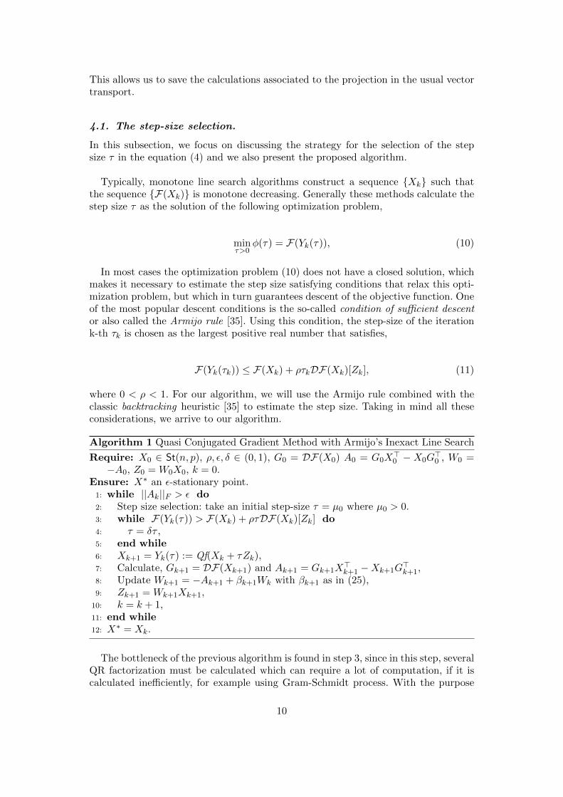
Algorithm 1 Quasi Conjugated Gradient Method with Armijo’s Inexact Line Search

Require: X0 ∈ St(n, p), ρ, ε, δ ∈ (0, 1), G0 = DF(X0) A0 = G0X>0 − X0G

>0 , W0 =

−A0, Z0 = W0X0, k = 0.Ensure: X∗ an ε-stationary point.

1: while ||Ak||F > ε do2: Step size selection: take an initial step-size τ = µ0 where µ0 > 0.3: while F(Yk(τ)) > F(Xk) + ρτDF(Xk)[Zk] do4: τ = δτ ,5: end while6: Xk+1 = Yk(τ) := Qf(Xk + τZk),7: Calculate, Gk+1 = DF(Xk+1) and Ak+1 = Gk+1X

>k+1 −Xk+1G

>k+1,

8: Update Wk+1 = −Ak+1 + βk+1Wk with βk+1 as in (25),9: Zk+1 = Wk+1Xk+1,

10: k = k + 1,11: end while12: X∗ = Xk.

The bottleneck of the previous algorithm is found in step 3, since in this step, severalQR factorization must be calculated which can require a lot of computation, if it iscalculated inefficiently, for example using Gram-Schmidt process. With the purpose

10

of reducing the computational cost of algorithm 1, we consider to compute the QRfactorization of the matrix M = Xk + τZk via Cholesky factorization. For this end,we use the following procedure,

Algorithm 2 QR factorization via Cholesky

Require: M ∈ Rn×p a matrix such that M>M is positive definite.Ensure: Q ∈ St(n, p) and R ∈ Rp×p upper-triangular matrix.

1: Compute the Cholesky factorization L>L of M>M where L ∈ Rp×p is a upper-triangular matrix.

2: Q = ML−1 and R = L

Note that, since Wk is skew-symmetric and Xk ∈ St(n, p), we haveM>M = Ip + τ2X>k W

>k WkXk, so, let v ∈ Rp be an arbitrary non-zero vector,

then v>M>k Mkv = ||v||2 + τ2||WkXkv||2 > 0, thus we conclude that M>M is apositive defined matrix. Therefore, the existence of the Cholesky factorization of suchmatrix is guaranteed.

Typically, the Riemannian conjugate gradient methods require that the step sizeτ satisfy the strong Wolfe conditions [35], (whose Riemannian version appear in[32,36]) in each iteration, and furthermore, the vector transport needs to satisfy thenon-expansive Ring-Wirth condition [36], to guarantee global convergence. By meansof a direct calculation, it can be verified that the vector transport given in (8) satisfiesthis condition for the case of n = p, nevertheless, when p < n, this condition is notnecessarily fulfilled. There are ways to rescale any vector transport to obtain anotherone that satisfies the Ring-Wirth condition [37].

However, if we allow the algorithm to periodically restart the direction by settingβk = 0, then we can guarantee that all these Zk are descent directions, and thenthe procedure becomes a line search method on matrix manifold. Observe that in ouralgorithm, we use this restart and in this way, we have that Zk gradient-relatedsequence that is contained in the bundle of the Stiefel manifold. In addition, themapping RXk

(ηk) := Qf(Xk + ηk) is a retraction, a proof of this fact is found in [27].Therefore, the results of global convergence that appear in [27] regarding line-searchmethods on manifolds using retractions apply directly to Algorithm 1, which allowsus to establish the following theorem.

Theorem 4.2. Let Xk be an infinite sequence of iterates generated by Algorithm 1,then

limk→∞

||∇eF(Xk)||F = 0.

Another important observation, is that our proposal also works with other retrac-tions different to that based on QR decomposition. For example, we can use ourproposal in combination with the Cayley transform to obtain the following updateformula,

Xk+1 = Y Cayleyk (τ) := (In +

τ

2Wk)

−1(In −τ

2Wk)Xk, (12)

this update scheme (12) would correspond to a modified version of the algorithm

11

proposed in [25]. We can also consider retractions based on exponential mapping andpolar decomposition in conjunction with our proposal, that is,

Xk+1 = Y Expk (τ) := exp(τWk)Xk, (13)

Xk+1 = Y Polark (τ) := (Xk + τWkXk)(Ip −X>k W 2

kXk)−1/2, (14)

respectively. Nevertheless, note that these update schemes (12)-(13)-(14) require tocompute matrix inversions of size n × n, calculate exponentials matrix or estimatematrix square roots, which become expensive calculations when the dimension of thematrix Xk is large. For this reason, we adopt the retraction based on the QR decom-position, because this can be calculated efficiently using the Algorithm 2.

5. Numerical Experiments

In this section, we perform some numerical experiments to investigate the efficiencyof the proposed method. All algorithms were implemented using MATLAB 7.10 ona intel(R) CORE(TM) i7-4770, CPU 3.40 GHz with 500 Gb of HD and 16 Gb ofRam. We present a comparative study of our algorithm versus other state-of-the-artalgorithms for several instances of the problems Joint diagonalization problem andTotal energy minimization generating synthetic data.

5.1. Terminating the Algorithm

The algorithms are terminated if we reach a point Xk on the Stiefel manifold thatsatisfies any of the following stopping criteria,

• k ≥ Kmax where Kmax is the maximum number of iterations allowed by theuser.• ||∇cF(Xk)||F ≤ ε, where ε ∈ (0, 1) is a given scalar.

• Err Relxk < tolx and Err Relfk < tolf , where tolx, tolf ∈ (0, 1).• mean(Err Relx1+k−min(k,T ), . . . ,Err Relxk]) ≤ 10 tolx and

mean([Err Relf1+k−min(k,T ), . . . ,Err Relfk ]) ≤ 10 tolf

where, the values Err Relxk and Err Relfk are defined by,

Err Relxk :=||Xk −Xk−1||F√

n, Err Relfk :=

|F(Xk)−F(Xk−1)||F(Xk−1)|+ 1

.

The default values for the parameters in our algorithms are: ε = 1e-5, tolx =1e-12, tolf = 1e-12, T = 5, Kmax = 1000, δ = 0.2, ρ1 = 1e-4, τm = 1e-20, τM = 1e+20.

In the rest of this section we will denote by: “Nitr” to the number of iterations,“Time” to CPU time in seconds, “Fval” to the value of the evaluated objective func-tion in the optimum estimated, “NrmG” to the norm of Gradient of the Lagrangean

12

function evaluated in the optimum estimate (||∇cF(X)||F ) and “Feasi” to the feasi-

bility error (||X>X − I||F ), obtained by the algorithms.

5.2. Joint diagonalization problem

The Joint diagonalization problem (JDP) for N matrices A1, A2,..., AN symmetric ofsize n× n, consists of finding an orthogonal matrix of size n× p, which minimizes thesum of the squares of the diagonal entries of the matrices X>AlX, l = 1, 2, . . . , N , orequivalently, maximize the sum of the squares of the entries of the diagonals of thematrices X>AlX, l = 1, 2, . . . , N , see [38]. Getting a solution for this problem (JDP)is of great value for applications such as Independent Component Analysis (ICA) andalso for The Blind Source Separation Problem among others (see [39]).

In [34,40] different methods on manifolds have been studied to solve the problemJDP on the Stiefel manifold, more specifically, consider the following problem:

minF(X) = −N∑l=1

||diag(X>AlX)||2F , s.a. X ∈ St(n, p), (15)

where A1, A2, ..., AN are real symmetric matrices of size n× n and where diag(Y ) isthe matrix whose main diagonal matches the main diagonal of the matrix Y and allother entries are zero.

In this subsection, we tested the efficiency of our algorithms when solving theproblem (15), and compared our procedure with two of the state-of-the-art methodsOptStiefel [25] and Grad retrac [30]. In the following tables, we show the average ofeach values to be compared in a total of 100 executions. In addition, the maximumnumber of iterations is set at 8000, we use a tolerance for the gradient norm of ε =1e-5 and we take the following values, xtol = 1e-14 and ftol = 1e-14 as tolerances forthe other stop criteria.

First, we perform an experiment varying p and n (this experiment was taken from[34]). In this case, we build the matrices A1, A2,..., AN as follows. We generateN = 10 randomly n × n diagonal matrices Λ1, Λ2,..., ΛN , and a randomly chosen

n× n orthogonal matrix P , where the diagonal entries λ(l)1 , λ

(l)2 ,..., λ

(l)n of each Λl are

positive and in descending order. We then put A1, A2,..., AN as Al = PΛlP> for all

l = 1, 2, ..., N . Observe that X∗ = PIn,p is an optimal solution to the problem (15).As a starting point, we compute an approximate solution X0 = Qf(X∗ + Xrand),where Xrand is a randomly chosen n× p matrix such that maxi,j|xij | ≤ 0.01, wherexij denotes the entry (i, j) of matrix Xrand.

The numerical results, associated with this experiment for several values of n andp, are contained in Table 1. From these table we can observe that, all the methodscompared show a similar performance in terms of CPU time, but our method performsmore iterations. However, the three algorithms get good solutions. In addition, inFigure 1, we illustrate the behavior of our proposed algorithm for a particularexecution with n = 50, p = 30 and N = 5, building the problem as explained at thebeginning of this paragraph.

13

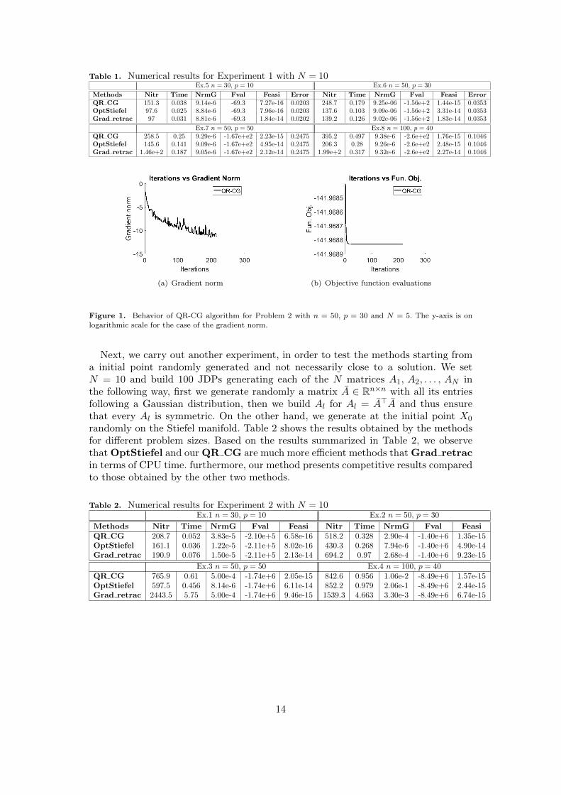
Table 1. Numerical results for Experiment 1 with N = 10Ex.5 n = 30, p = 10 Ex.6 n = 50, p = 30

Methods Nitr Time NrmG Fval Feasi Error Nitr Time NrmG Fval Feasi ErrorQR CG 151.3 0.038 9.14e-6 -69.3 7.27e-16 0.0203 248.7 0.179 9.25e-06 -1.56e+2 1.44e-15 0.0353OptStiefel 97.6 0.025 8.84e-6 -69.3 7.96e-16 0.0203 137.6 0.103 9.09e-06 -1.56e+2 3.31e-14 0.0353Grad retrac 97 0.031 8.81e-6 -69.3 1.84e-14 0.0202 139.2 0.126 9.02e-06 -1.56e+2 1.83e-14 0.0353

Ex.7 n = 50, p = 50 Ex.8 n = 100, p = 40QR CG 258.5 0.25 9.29e-6 -1.67e+e2 2.23e-15 0.2475 395.2 0.497 9.38e-6 -2.6e+e2 1.76e-15 0.1046OptStiefel 145.6 0.141 9.09e-6 -1.67e+e2 4.95e-14 0.2475 206.3 0.28 9.26e-6 -2.6e+e2 2.48e-15 0.1046Grad retrac 1.46e+2 0.187 9.05e-6 -1.67e+e2 2.12e-14 0.2475 1.99e+2 0.317 9.32e-6 -2.6e+e2 2.27e-14 0.1046

(a) Gradient norm (b) Objective function evaluations

Figure 1. Behavior of QR-CG algorithm for Problem 2 with n = 50, p = 30 and N = 5. The y-axis is onlogarithmic scale for the case of the gradient norm.

Next, we carry out another experiment, in order to test the methods starting froma initial point randomly generated and not necessarily close to a solution. We setN = 10 and build 100 JDPs generating each of the N matrices A1, A2, . . . , AN inthe following way, first we generate randomly a matrix A ∈ Rn×n with all its entriesfollowing a Gaussian distribution, then we build Al for Al = A>A and thus ensurethat every Al is symmetric. On the other hand, we generate at the initial point X0

randomly on the Stiefel manifold. Table 2 shows the results obtained by the methodsfor different problem sizes. Based on the results summarized in Table 2, we observethat OptStiefel and our QR CG are much more efficient methods that Grad retracin terms of CPU time. furthermore, our method presents competitive results comparedto those obtained by the other two methods.

Table 2. Numerical results for Experiment 2 with N = 10Ex.1 n = 30, p = 10 Ex.2 n = 50, p = 30

Methods Nitr Time NrmG Fval Feasi Nitr Time NrmG Fval FeasiQR CG 208.7 0.052 3.83e-5 -2.10e+5 6.58e-16 518.2 0.328 2.90e-4 -1.40e+6 1.35e-15OptStiefel 161.1 0.036 1.22e-5 -2.11e+5 8.02e-16 430.3 0.268 7.94e-6 -1.40e+6 4.90e-14Grad retrac 190.9 0.076 1.50e-5 -2.11e+5 2.13e-14 694.2 0.97 2.68e-4 -1.40e+6 9.23e-15

Ex.3 n = 50, p = 50 Ex.4 n = 100, p = 40QR CG 765.9 0.61 5.00e-4 -1.74e+6 2.05e-15 842.6 0.956 1.06e-2 -8.49e+6 1.57e-15OptStiefel 597.5 0.456 8.14e-6 -1.74e+6 6.11e-14 852.2 0.979 2.06e-1 -8.49e+6 2.44e-15Grad retrac 2443.5 5.75 5.00e-4 -1.74e+6 9.46e-15 1539.3 4.663 3.30e-3 -8.49e+6 6.74e-15

14

5.3. Total energy minimization

In this subsection, we consider a version of the total energy minimization problem:

minX∈Rn×k

Etotal(X) =1

2Tr[X>LX] +

µ

4ρ(X)>L†ρ(X) s.t. X>X = I (16)

where L is a discrete Laplacian operator, µ > 0 is a constant, L† denote the Moore-Penrose generalized inverse of L and ρ(X) := diag(XX>) is the vector containing thediagonal elements of the matrix XX>. The problem (16) is a simplified version of theHartreeFock (HF) total energy minimization problem and the Kohn-Sham (KS) totalenergy minimization problem in electronic structure calculations (see for details [41–44]). The first order necessary conditions for the total energy minimization problem(16) are given by:

H(X)X −XΛ = 0 (17)

X>X = I, (18)

where H(X) := L+ µDiag(L†ρ(X)) and Λ is the Lagrange multipliers matrix. Here,the symbol Diag(x) is a diagonal matrix with a vector x on its diagonal. Observethat the equations (17)-(18) can be seen as a nonlinear eigenvalue problem.

The experiments 1.1-1.2 described below were taken from [42], we replay theexperiments over 100 different starting points, moreover, we use a maximum numberof iterations K = 4000 and tolerance of ε = 1e-5. To show the efficacy of our methodssolving the problem (16), we present the numerical results for problems 1.1-1.2 withdifferent choices of n, k, and µ. In this subsection, we compare the Algorithm 1 withthe Steepest Descent method (Steep-Dest), Trust-Region method (Trust-Reg) andConjugate Gradient method (Conj-Grad) from manopt toolbox, see Ref. [45]1.

Experiment 1.1 [42]: We consider the nonlinear eigenvalue problem for k = 10;µ = 1, and varying n = 200, 400, 800, 1000.

Experiment 1.2 [42]: We consider the nonlinear eigenvalue problem for n = 100and k = 20 and varying µ.

In all these testing, the L matrix that appears in the problem (16) is built as theone-dimensional discrete Laplacian with 2 on the diagonal and 1 on the sub- andsup-diagonals.

The results corresponding to the experiment 1.1 are presented in Table 3. We seefrom this table that our method (QR CG) is more efficient than the rest of thealgorithms when n is small, but if n is moderately large then Conj-Grad becomesthe best algorithm for this specific application. However, all methods obtain similarresults in terms of the gradient norm (NrmG) and the optimal objective value (Fval).

Table 4 lists numerical results for Example 1.2. In this table, we note that ourprocedure gets better performance than the others methods, due to our QR CG

1The tool-box manopt is available in http://www.manopt.org/

15

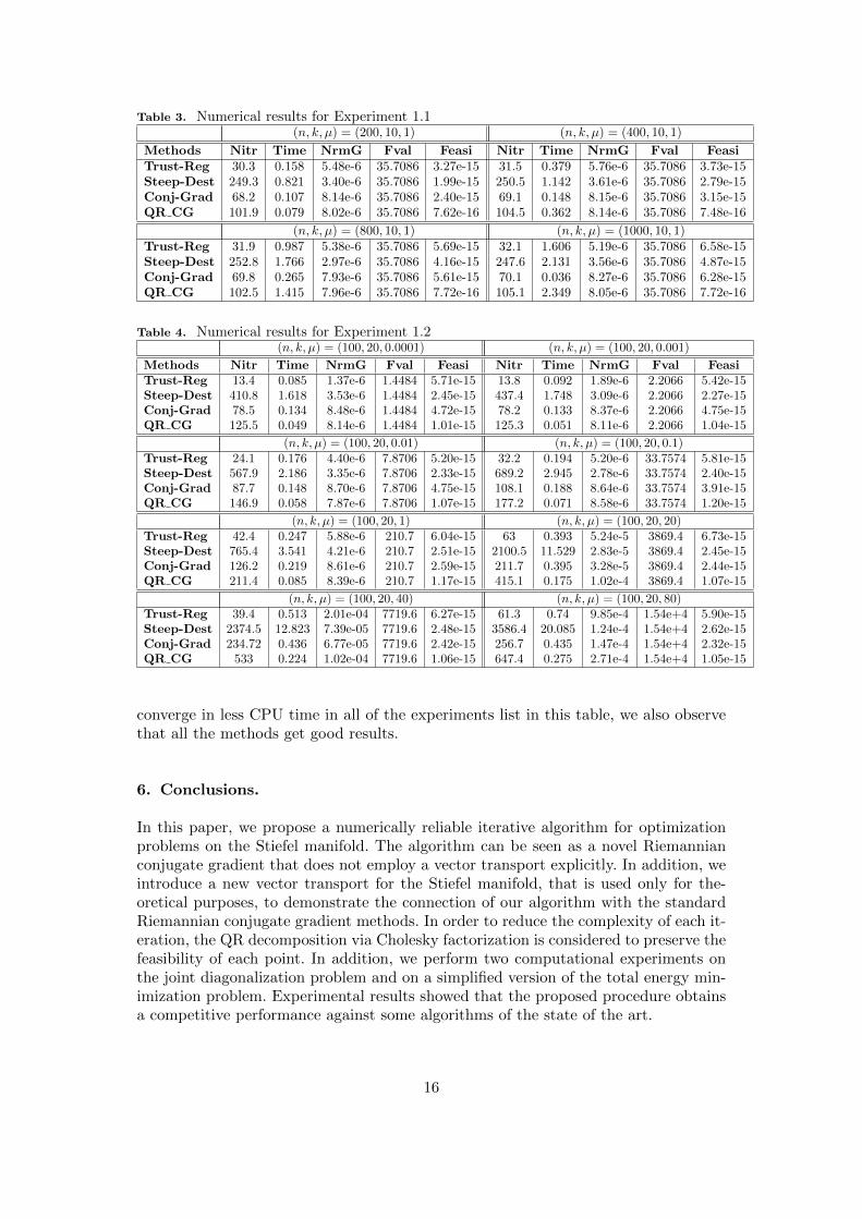
Table 3. Numerical results for Experiment 1.1(n, k, µ) = (200, 10, 1) (n, k, µ) = (400, 10, 1)

Methods Nitr Time NrmG Fval Feasi Nitr Time NrmG Fval FeasiTrust-Reg 30.3 0.158 5.48e-6 35.7086 3.27e-15 31.5 0.379 5.76e-6 35.7086 3.73e-15Steep-Dest 249.3 0.821 3.40e-6 35.7086 1.99e-15 250.5 1.142 3.61e-6 35.7086 2.79e-15Conj-Grad 68.2 0.107 8.14e-6 35.7086 2.40e-15 69.1 0.148 8.15e-6 35.7086 3.15e-15QR CG 101.9 0.079 8.02e-6 35.7086 7.62e-16 104.5 0.362 8.14e-6 35.7086 7.48e-16

(n, k, µ) = (800, 10, 1) (n, k, µ) = (1000, 10, 1)Trust-Reg 31.9 0.987 5.38e-6 35.7086 5.69e-15 32.1 1.606 5.19e-6 35.7086 6.58e-15Steep-Dest 252.8 1.766 2.97e-6 35.7086 4.16e-15 247.6 2.131 3.56e-6 35.7086 4.87e-15Conj-Grad 69.8 0.265 7.93e-6 35.7086 5.61e-15 70.1 0.036 8.27e-6 35.7086 6.28e-15QR CG 102.5 1.415 7.96e-6 35.7086 7.72e-16 105.1 2.349 8.05e-6 35.7086 7.72e-16

Table 4. Numerical results for Experiment 1.2(n, k, µ) = (100, 20, 0.0001) (n, k, µ) = (100, 20, 0.001)

Methods Nitr Time NrmG Fval Feasi Nitr Time NrmG Fval FeasiTrust-Reg 13.4 0.085 1.37e-6 1.4484 5.71e-15 13.8 0.092 1.89e-6 2.2066 5.42e-15Steep-Dest 410.8 1.618 3.53e-6 1.4484 2.45e-15 437.4 1.748 3.09e-6 2.2066 2.27e-15Conj-Grad 78.5 0.134 8.48e-6 1.4484 4.72e-15 78.2 0.133 8.37e-6 2.2066 4.75e-15QR CG 125.5 0.049 8.14e-6 1.4484 1.01e-15 125.3 0.051 8.11e-6 2.2066 1.04e-15

(n, k, µ) = (100, 20, 0.01) (n, k, µ) = (100, 20, 0.1)Trust-Reg 24.1 0.176 4.40e-6 7.8706 5.20e-15 32.2 0.194 5.20e-6 33.7574 5.81e-15Steep-Dest 567.9 2.186 3.35e-6 7.8706 2.33e-15 689.2 2.945 2.78e-6 33.7574 2.40e-15Conj-Grad 87.7 0.148 8.70e-6 7.8706 4.75e-15 108.1 0.188 8.64e-6 33.7574 3.91e-15QR CG 146.9 0.058 7.87e-6 7.8706 1.07e-15 177.2 0.071 8.58e-6 33.7574 1.20e-15

(n, k, µ) = (100, 20, 1) (n, k, µ) = (100, 20, 20)Trust-Reg 42.4 0.247 5.88e-6 210.7 6.04e-15 63 0.393 5.24e-5 3869.4 6.73e-15Steep-Dest 765.4 3.541 4.21e-6 210.7 2.51e-15 2100.5 11.529 2.83e-5 3869.4 2.45e-15Conj-Grad 126.2 0.219 8.61e-6 210.7 2.59e-15 211.7 0.395 3.28e-5 3869.4 2.44e-15QR CG 211.4 0.085 8.39e-6 210.7 1.17e-15 415.1 0.175 1.02e-4 3869.4 1.07e-15

(n, k, µ) = (100, 20, 40) (n, k, µ) = (100, 20, 80)Trust-Reg 39.4 0.513 2.01e-04 7719.6 6.27e-15 61.3 0.74 9.85e-4 1.54e+4 5.90e-15Steep-Dest 2374.5 12.823 7.39e-05 7719.6 2.48e-15 3586.4 20.085 1.24e-4 1.54e+4 2.62e-15Conj-Grad 234.72 0.436 6.77e-05 7719.6 2.42e-15 256.7 0.435 1.47e-4 1.54e+4 2.32e-15QR CG 533 0.224 1.02e-04 7719.6 1.06e-15 647.4 0.275 2.71e-4 1.54e+4 1.05e-15

converge in less CPU time in all of the experiments list in this table, we also observethat all the methods get good results.

6. Conclusions.

In this paper, we propose a numerically reliable iterative algorithm for optimizationproblems on the Stiefel manifold. The algorithm can be seen as a novel Riemannianconjugate gradient that does not employ a vector transport explicitly. In addition, weintroduce a new vector transport for the Stiefel manifold, that is used only for the-oretical purposes, to demonstrate the connection of our algorithm with the standardRiemannian conjugate gradient methods. In order to reduce the complexity of each it-eration, the QR decomposition via Cholesky factorization is considered to preserve thefeasibility of each point. In addition, we perform two computational experiments onthe joint diagonalization problem and on a simplified version of the total energy min-imization problem. Experimental results showed that the proposed procedure obtainsa competitive performance against some algorithms of the state of the art.

16

Acknowledgements

This work was supported in part by CONACYT (Mexico).

References

[1] Gilles Meyer, Silvere Bonnabel, and Rodolphe Sepulchre. Linear regression under fixed-rank constraints: a riemannian approach. In Proceedings of the 28th international confer-ence on machine learning, 2011.

[2] Emmanuel J Candes and Benjamin Recht. Exact matrix completion via convex optimiza-tion. Foundations of Computational mathematics, 9(6):717, 2009.

[3] Bart Vandereycken. Low-rank matrix completion by riemannian optimization. SIAMJournal on Optimization, 23(2):1214–1236, 2013.

[4] Hugo Lara, Harry Oviedo, and Jinjun Yuan. Matrix completion via a low rank factoriza-tion model and an augmented lagrangean succesive overrelaxation algorithm. Bulletin ofComputational Applied Mathematics, CompAMa, 2(2):21–46, 2014.

[5] Xin Zhang, Jinwei Zhu, Zaiwen Wen, and Aihui Zhou. Gradient type optimizationmethods for electronic structure calculations. SIAM Journal on Scientific Computing,36(3):C265–C289, 2014.

[6] P-A Absil and Kyle A Gallivan. Joint diagonalization on the oblique manifold for inde-pendent component analysis. In Acoustics, Speech and Signal Processing, 2006. ICASSP2006 Proceedings. 2006 IEEE International Conference on, volume 5, pages V–V. IEEE,2006.

[7] Xiaowen Dong, Pascal Frossard, Pierre Vandergheynst, and Nikolai Nefedov. Clusteringon multi-layer graphs via subspace analysis on grassmann manifolds. IEEE Transactionson signal processing, 62(4):905–918, 2014.

[8] Michel Journee, Francis Bach, P-A Absil, and Rodolphe Sepulchre. Low-rank optimizationon the cone of positive semidefinite matrices. SIAM Journal on Optimization, 20(5):2327–2351, 2010.

[9] Petros T Boufounos and Richard G Baraniuk. 1-bit compressive sensing. In InformationSciences and Systems, 2008. CISS 2008. 42nd Annual Conference on, pages 16–21. IEEE,2008.

[10] Youcef Saad. Numerical methods for large eigenvalue problems. Manchester UniversityPress, 1992.

[11] Zaiwen Wen, Chao Yang, Xin Liu, and Yin Zhang. Trace-penalty minimization for large-scale eigenspace computation. Journal of Scientific Computing, 66(3):1175–1203, 2016.

[12] JB Francisco and Tiara Martini. Spectral projected gradient method for the procrustesproblem. TEMA (Sao Carlos), 15(1):83–96, 2014.

[13] Peter H Schonemann. A generalized solution of the orthogonal procrustes problem. Psy-chometrika, 31(1):1–10, 1966.

[14] Thomas Viklands. Algorithms for the weighted orthogonal Procrustes problem and otherleast squares problems. PhD thesis, Datavetenskap, 2006.

[15] Renee T Meinhold, Tyler L Hayes, and Nathan D Cahill. Efficiently computing piece-wise flat embeddings for data clustering and image segmentation. arXiv preprintarXiv:1612.06496, 2016.

[16] Mihai Cucuringu, Yaron Lipman, and Amit Singer. Sensor network localization by eigen-vector synchronization over the euclidean group. ACM Transactions on Sensor Networks(TOSN), 8(3):19, 2012.

[17] Davide Eynard, Klaus Glashoff, Michael M Bronstein, and Alexander M Bronstein.Multimodal diffusion geometry by joint diagonalization of laplacians. arXiv preprintarXiv:1209.2295, 2012.

[18] Donald Goldfarb, Zaiwen Wen, and Wotao Yin. A curvilinear search method for p-

17

harmonic flows on spheres. SIAM Journal on Imaging Sciences, 2(1):84–109, 2009.[19] Effrosini Kokiopoulou, Jie Chen, and Yousef Saad. Trace optimization and eigenproblems

in dimension reduction methods. Numerical Linear Algebra with Applications, 18(3):565–602, 2011.

[20] Constantin Udriste. Convex functions and optimization methods on Riemannian mani-folds, volume 297. Springer Science & Business Media, 1994.

[21] Steven T Smith. Optimization techniques on riemannian manifolds. Fields institutecommunications, 3(3):113–135, 1994.

[22] Robert Mahony. Optimization algorithms on homogeneous spaces. PhD thesis, PhD thesis,Australian National University, Canberra, 1994.

[23] Alan Edelman, Tomas A Arias, and Steven T Smith. The geometry of algorithms withorthogonality constraints. SIAM journal on Matrix Analysis and Applications, 20(2):303–353, 1998.

[24] Jonathan H Manton. Optimization algorithms exploiting unitary constraints. IEEETransactions on Signal Processing, 50(3):635–650, 2002.

[25] Zaiwen Wen and Wotao Yin. A feasible method for optimization with orthogonalityconstraints. Mathematical Programming, 142(1-2):397–434, 2013.

[26] Traian E Abrudan, Jan Eriksson, and Visa Koivunen. Steepest descent algorithms foroptimization under unitary matrix constraint. IEEE Transactions on Signal Processing,56(3):1134–1147, 2008.

[27] P-A Absil, Robert Mahony, and Rodolphe Sepulchre. Optimization algorithms on matrixmanifolds. Princeton University Press, 2009.

[28] Oscar Susano Dalmau Cedeno and Harry Fernando Oviedo Leon. Projected nonmono-tone search methods for optimization with orthogonality constraints. Computational andApplied Mathematics, pages 1–27, 2017.

[29] Oscar Dalmau-Cedeno and Harry Oviedo. A projection method for optimization problemson the stiefel manifold. In Mexican Conference on Pattern Recognition, pages 84–93.Springer, 2017.

[30] Harry Oviedo, Hugo Lara, and Oscar Dalmau. A non-monotone linear search algorithmwith mixed direction on stiefel manifold. Optimization Methods and Software, 0(0):1–21,2018.

[31] Traian Abrudan, Jan Eriksson, and Visa Koivunen. Conjugate gradient algorithm foroptimization under unitary matrix constraint. Signal Processing, 89(9):1704–1714, 2009.

[32] Xiaojing Zhu. A riemannian conjugate gradient method for optimization on the stiefelmanifold. Computational Optimization and Applications, 67(1):73–110, 2017.

[33] Chunhong Qi, Kyle A Gallivan, and Pierre-Antoine Absil. An efficient bfgs algorithmfor riemannian optimization. In Proceedings of the 19th International Symposium onMathematical Theory of Network and Systems (MTNS 2010), volume 1, pages 2221–2227,2010.

[34] Hiroyuki Sato. Riemannian newton’s method for joint diagonalization on the stiefel man-ifold with application to ica. arXiv preprint arXiv:1403.8064, 2014.

[35] Jorge Nocedal and Stephen J Wright. Numerical optimization 2nd, 2006.[36] Wolfgang Ring and Benedikt Wirth. Optimization methods on riemannian manifolds and

their application to shape space. SIAM Journal on Optimization, 22(2):596–627, 2012.[37] Hiroyuki Sato and Toshihiro Iwai. A new, globally convergent riemannian conjugate

gradient method. Optimization, 64(4):1011–1031, 2015.[38] Mati Wax and Jacob Sheinvald. A least-squares approach to joint diagonalization. IEEE

Signal Processing Letters, 4(2):52–53, 1997.[39] Bijan Afsari and Perinkulam S Krishnaprasad. Some gradient based joint diagonalization

methods for ica. In ICA, volume 3195, pages 437–444. Springer, 2004.[40] Fabian J Theis, Thomas P Cason, and Pierre-Antoine Absil. Soft dimension reduction

for ica by joint diagonalization on the stiefel manifold. In ICA, pages 354–361. Springer,2009.

[41] Richard M Martin. Electronic structure: basic theory and practical methods. Cambridge

18

university press, 2004.[42] Zhi Zhao, Zheng-Jian Bai, and Xiao-Qing Jin. A riemannian newton algorithm for nonlin-

ear eigenvalue problems. SIAM Journal on Matrix Analysis and Applications, 36(2):752–774, 2015.

[43] Chao Yang, Juan C Meza, and Lin-Wang Wang. A constrained optimization algorithm fortotal energy minimization in electronic structure calculations. Journal of ComputationalPhysics, 217(2):709–721, 2006.

[44] Chao Yang, Juan C Meza, and Lin-Wang Wang. A trust region direct constrained mini-mization algorithm for the kohn–sham equation. SIAM Journal on Scientific Computing,29(5):1854–1875, 2007.

[45] Nicolas Boumal, Bamdev Mishra, Pierre-Antoine Absil, Rodolphe Sepulchre, et al.Manopt, a matlab toolbox for optimization on manifolds. Journal of Machine Learn-ing Research, 15(1):1455–1459, 2014.

19