A review of parametric modelling techniques for EEG analysisnin/Courses/Seminar14a/ARmodels.pdf ·...

ELSEVIER 1350-4533(95)000240

Med. Eng, Phys. Vol. 18, No. 1, pp. 2-11, 1996 Copyright 0 1995 Elsevier Science Ltd for IPEMB

Printed in Great Britain. All rights reserved 135&4533/96 $15.00 + 0.00

Review

A review of parametric modelling techniques for EEG analysis

J. Pardey*, S. Roberts+ and L. Tarassenko*

*Universi 7

of Oxford, Medical Engineering Unit, 43 Banbury Road, Oxford OX2 6PE, UK, Imperial College of Science, Technology & Medicine, Exhibition Road, London SW7 2BT, UK

Received 27 January 1995, accepted 24 March 1995

ABSTRACT This review provides an introduction to the use ofparametric modelling techniques f&r time series analysis, and in

particular the application of autoregressive modelling to the analysis of physiological sign& such as the human

electroencephalogram. The concept of signal stationarity is considered and, in the light of this, both adaptive models,

and non-adaptive models employing fixed or adaptive segmentation, are discussed. For non-adaptive autoregressive

models, the Yule-Walker equations are o!erived and the popular Levinson-Durbin and Burg algorithms are intro-

duced. The interpretation of an autoregressive model as a recursive digital jilter and its use in spectral estimation

are considered, and the important issues of model stability and model complexity are discussed.

Keywords: Autoregressive modelling, biomedical signal processing, human sleep EEG

Med. Eng. Phys., 1996, Vol. 18, 2-11, January

1. INTRODUCTION

Parametric modelling is a technique for time series analysis in which a mathematical model is fitted to a sampled signal. If the model forms a good approximation to the signal’s observed behavior it can then be used in a wide range of applications, such as spectral estimation, linear prediction coding (LPC) for data compression, speech synthesis, and feature extraction for pattern classification problems.

The mathematical model that is most widely used is a rational transfer function, the exact form of which is determined by estimating suitable values for its free parameters. If all of these parameters lie in the transfer function’s denominator then the model is termed an all-pole or autorepss- ive (AR) model, while an all-zero or moving-average (MA) model has all of its free parameters in the numerator. A model with free parameters in both the numerator and denominator is then termed a pole-zero or autoregressive moving-average (ARMA) model.

Furthermore, in adaptive models the values of the free parameters are updated with the arrival of each new data sample, whereas in non-adaptive models the parameters are chosen so as to give

the best fit to a sequence of data samples. Because of this, non-adaptive models require that the signal is stationq, i.e. that its statistical character- istics, such as average amplitude and frequency content, do not vary with time. Most signals, including speech and the electroencephalogram (EEG) , are non-stationary (i.e. they have a time- varying frequency spectrum), although they can be considered locally stationary over short time intervals. For such signals, either an adaptive model can be used, or the signal can be divided into sufficiently short, quasi-stationary segments and a non-adaptive model fitted to each segment. The length of these segments can be either fixed, typically at 1 s for EEG analysis, or variable, in which case the signal is continuously monitored for departures from stationarity and segment boundaries are placed accordingly.’

The key to the performance of parametric modelling techniques, however, lies in the relative effectiveness of the various algorithms that can be used to estimate the free parameters. For non- adaptive AR models the two most popular algorithms are the Levinson-Durbin algorithm and the Burg algorithm, while for adaptive AR models the Kalman filtering algorithm2*3 is commonly used. This is summarized in Figure 1.

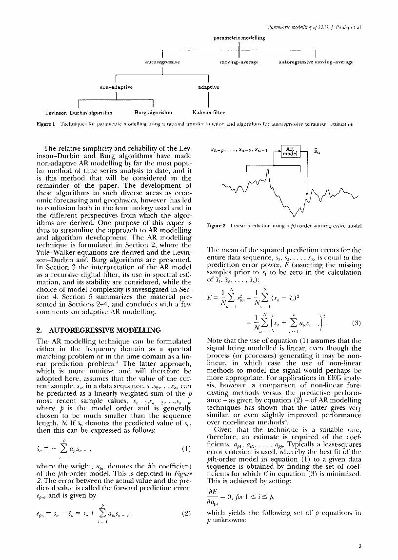
I autoregressive

I moving-average

I autoregressive moving-average

non-adaptive adaptive

Levinson-Durbin algorithm Burg algorithm Kalman filter

Figure 1 ‘l‘rchniqurc for parametric modelling using a rational tlanufrr function and algorithms for autoqrcssivr parameter rrtimation

The relative simplicity and reliability of the Lev- inson-Durbin and Burg algorithms have made non-adaptive AR modelling by far the most popu-

lar method of time series analysis to date, and it is this method that will be considered in the remainder of the paper. The development of these algorithms in such diverse areas as econ- omic forecasting and geophysics, however, has led to confusion both in the terminology used and in the different perspectives from which the algorithms are derived. One purpose of this paper is thus to streamline the approach to AR modelling and algorithm development. The AR modelling technique is formulated in Section 2, where the Yule-Walker equations are derived and the Levin- son-Durbin and Burg algorithms are presented. In Section 3 the interpretation of the AR model as a recursive digital filter, its use in spectral estimation, and its stability are considered, while the choice of model complexity is investigated in Sec- tion 4. Section 5 summarizes the material presented in Sections 2-4, and concludes with a few comments on adaptive AR modelling.

2. AUTOREGRESSIVE MODELLING

The AR modelling technique can be formulated either in the frequency domain as a spectral matching problem or in the time domain as a linear prediction problem.” The latter approach, which is more intuitive and will therefore be adopted here, assumes that the value of the current sample, s,,, in a data sequence, s,,s,,. . .,s,~, can be predicted as a linearly weighted sum of the p most recent sample values, s,, _ ,,s,, ~ ?,. . .,s,, ,, where p is the model order and is general y r chosen to be much smaller than the sequence length, N. If $, denotes the predicted value of s,,, then this can be expressed as follows:

s;, = - i a,,,s,, ,, (1) I I

where the weight, nPi, denotes the ith coefficient of the pth-order model. This is depicted in &JUTP 2. The error between the actual value and the predicted value is called the forward prediction error, P,,,, and is given by

The mean of the squared prediction errors for the entire data sequence, s,, s:, . . . , .s,~, is equal to the prediction error power, E, (assuming the missing samples prior to s, to be zero in the calculation of 5,) 32, . . . , T,,):

Note that the use of equation (1) assumes that the signal being modelled is linear, even though the process (or processes) generating it may be non- linear, in which case the use of non-linear methods to model the signal would perhaps be more appropriate. For applications in EEG analysis, however, a comparison of non-linear forecasting methods versus the predictive performance - as given by equation (2) - of AR modelling techniques has shown that the latter gives very similar, or even slightly improved performance over non-linear methods’.

Given that the technique is a suitable one, therefore, an estimate is required of the coefficients, a,,,,, spy, . . . , u~$,. Typically a least-squares error criterion is used, whereby the best fit of the @h-order model in equation (1) to a given data sequence is obtained by finding the set of coefficients for which E in equation (3) is minimized. This is achieved by setting:

which yields the following set of p equations in p unknowns:

3

Parametric modelling of FXG: J. Pardq et al.

(4)

Solving these for all, up2, . . . , upl, and substituting the values obtained back into equation (3) gives an expression for the minimum prediction error power, denoted by Et,:

However, given that the autocorrelation function of an infinite date sequence, SK,,. . . ,s,, is given by:

R, = pj!$% s,s, - i, for ---co < i <co, cc

n=l

where & = Ri (i.e. an even function of i) if the data sequence is stationary, so the parenthetic terms in (4) and (5) are just estimates of the first p + 1 terms of the truncated autocorrelation function, &, R1, . . . , f$,, using only the finite data sequence, s], s2, , . . , sN:

for05 ispand 1 ‘jlp,. (6)

where the missing samples prior to s1 are assumed to be-zero, as in (3). The use of 1 i - ~1 indicates that & -II depends on the difference between i and j (assuming stationarity) and not on their individual values. Substituting the values of &, RI,

5) , and . , &, obtained using (6) into (4) and (, rearranging (4) in matrix form gives:

& . . . &

I$ . . . R?

4

(7)

The error between the actual value and the predicted value in this case is called the backward p-e- diction error, bpn:

P Alternatively, the matrix equation in (7) can be augmented to include the expression for Ep:

bpn = s, ~ p - s;, - p = sn - p + c +A ~ p + ? (9) i= 1

1

UP1

UP2

UPP

-%

0

= 0

0

- (8)

Equations (7) or (8) are called the Y&J-WulFzer equations, and describe the p unknown AR coefficients in terms of the p + 1 estimated autocorrelation coefficients. Solving the Yule-Walker equations for upl, up2, . . ., upp is termed the uutocomelution method of AR parameter estimation and can be accomplished using a standard technique such as Gaussian elimination6 or a recursive technique such as the Levinson-Durbin ulgor- ithm4. The latter approach is computationally more efficient since it exploits the fact that the autocorrelation matrix on the left-hand side of equation (7) or (8) is both symmetric and a Toe- plitz matrix (i.e. the terms along any diagonal are the same). The algorithm, which is shown in Fig- ure 3, solves the Yule-Walker equations for each value of the model order from m = 0 to m = p. On each pass through the algorithm the estimated autocorrelation coefficients are used to generate a single, new coefficient, umm. The remaining coefficients, a,,, um2, . . . , umcm - ri, are then generated recursively from their (m - 1) th-order values, a(,- 1)lY qm- 1)2, . . . 7 qm- l)(m- l)? which are known from the previous pass through the algorithm. The expression for umj in Figure 3 is called the Levinson recursion, and will be used again later on.

The algorithm thus calculates the parameter sets, L%l, {all, 41, {a21, Q+,,, &A, and so on, for all of the lower order fits, m < p, to the data until the desired solution, {a ,, up2, . . . , a#, Ep], is obtained. Note that m = 0 escribes a zeroth-order model cf which does no prediction at all, so that E;, is simply the power in the data sequence, sl, s,, . . . , sN, and this in turn is equal to the zeroth autocorrelation coefficient, &, in equation (6). The intermediate values, k,, in Figure 3 are called the rejection, or partial correlation (PARCOR) coefficients, and can be interpreted as the partial correlation between s, and s~+~ holding s,+~, s,+~, . . . . sn+m-l constant.

Once the coefficients, upI, upz, . . . , upp, have been obtained, the AR model can be applied to the same data sequence, s,, s,, . . . , s,, but in the reverse direction. This is shown in Figure 4, where the value of the sample, s,- “predicted” as a linearly werg 3

is retrospectively ted sum of the p

future samples, s,+,+ 1, s, _ p + 2, . . ., s,:

fnep = - f: upisn-p+?

i= 1

4

Initialisation :

For rn = 1,2, . ..?p.

m-l

I;, zz - km’+ C a(m-l);Rm-i Em-1 i=l I/

Gnrn = km

ami = a(m-l)i + atnma(m-1)(,-i), for 1 < i < m - 1

Em = (I- k,$%-1

Figure 3 The I,winson-Durbin algorithm

Figure 4 Forward and backward linrar prediction

(Note that although this describes the prediction error for S, p it is denoted by b

cr and not

b!,(” - PI as might intuitively be expecte , this pecul- iar notation is just a mathematical convenience to simplify the expressions that follow.) Further- more, the fact that the AR coefficients were generated using the Levinson recursion in J@-ure 3 enables the following recursive relationships to be derived (see Appendix) between the forward prediction error in equation (2) and the backward prediction error in equation (9):

f? pn = “cp 1 ) N + appb,l, - I)(?, I) (10)

b,,, = b,,, I ) ( ,I I 1 + al,p7 ,, ~ I ) ,). (11)

These relationships express the pth-order prediction errors for s, and s,~ ~ ,,, in terms of their corresponding (p - 1) th-order prediction errors, and lead to a second, superior technique for AR parameter estimation called the maximum entropy method (MEM). Like the autocorrelation method described above, the maximum entropy method is a recursive estimation technique based on a least- squares error criterion. However, in the derivation of the Yule-Walker equations, the range of the summatiqn in the expressions for E in equation (3) and 4, il in equation (6) implicitly assumes

that the data outside the interval, s,, sZ, . . . , sh,, are zero. Since this is almost always an unrealistic assumption, the maximum entropy method restricts the range of the summation so as to use only the available data. Furthermore, instead of minimizing only the forward prediction error power, the maximum entropy method seeks to minimize the mean of both the forward and backward prediction error powers:

fi,‘ = 1-- A’ c (f$,, + $,J, 2(N- P),, = ,,+ , (15.3

subject to the constraint that the AR coefficients are updated using the Levinson recursion. This constraint enables the recursive relationships in equations (10) and (11) to be used, so that equation (12) can be expanded as follows:

1 .‘I

I:‘= 2(N- p) ~ __--- c (b,, I ) I, + ~~pp4p 1 ) (II I 1 I 2

n ! ’ + ’ + [b,,, I) (,I - 1, + $+,/‘QJ - 1) ,!I ‘1. This is a function of the unknown coefficient, a#, and the (p - 1) th-order forward and backward prediction errors, which are known from the previous pass through the algorithm. b: can thus be minimized by setting:

which yields

Using equation (13) in place of the corresponding expression in the Levinson-Durbin algorithm and adding the extra recursions for rP,& and bpn yields the Burg algorithm’ shown in FQure 5. An

5

Parametric modelling of FXG: J. Pardq et al.

Initialisation :

eon = bon = sn, for l<n<N

For m= 1,2,...,p:

N N

km = -2 C b(m--l)(n--l)qm-lfn

I c [b&x-1)(,-l) + gn-1)7&l

n=m+l n=m+l

am, = km

ami = a(,-1)i + %ma(m-l)(m-i), for l<i<m-1

Em = (l- k,!$&,-l

emn = q,-l), + ammb(m-l)(n-l~, for l<n<N-m

b mn = +,-1)(,+-l) + amme(m-l)n, for I<n<N-m

Figure 5 The Burg algorithm

additional step can also be included in the Burg algorithm that .reduces the computational complexity of equation (13) by calculating the denominator recursively?

denP = dena- 1[1 - a$- l)(P- 1) 1

- ?p- l)(N-p) - 4P- l)P’ where den,, = 2&Nfrom equations (12) and (13).

ePn

3. SPECTRAL ESTIMATION AND MODEL STABILITY

By rearranging the expression for the forward prediction error in equation (2) the AR model can be viewed as an all-pole, or infinite-impulse-response (IIR) filter whose current output, s,, is a function of both the p most recent outputs, S, _ 1, s, - 2, . . ., % - p’ and the current input, e*:

s, = S;, + epn = - 9 upis, - j + epn. (14) i= 1

This is shown in Figure 6. For applications such as EEG analysis, where the output signal is the observed EEG, the input signal is inaccessible and hence unknown. However, if the assumption made at the beginning of the previous section is correct (i.e. that s, is predictable from a linearly weighted sum of S, - 1, h-2, * * * 9 S, - p.), then the predicted values, $, %, . . . , &, can be Interpreted as the true, underlying signal, while the actual values, sl, s,, . . . , s,, can be regarded as these predicted values corrupted by additive white noise which, being uncorrelated and therefore unpre- dictable, gives rise to the prediction errors,

Figure 6 The interpretation of an autoregressive model as an all- pole filter

epl, ep2, . . -, epM The assumption just referred to can thus be rephrased with respect to Figure 6, in which it is assumed that the output sequence, Sl, $2, * * * , s,, is the result of using a pth-order AR model to filter a white noise input sequence, epl, ez,. . . , eN-

d $ It follows that when fitting an AR

mo el to a ata sequence, any departure of the prediction errors away from a white noise sequence can be used to indicate the goodness of fit of the model to the signal.

Despite this observation, it is a commonly held misconception that the application of AR modelling to EEG analysis is useful even if the prediction errors are correlated, since they can then be interpreted as the underlying “input signal” which, when filtered by the AR model, produces the observed EEG. This physiological interpretation of the AR model-whereby both the filter charac- teristics and the input signal are simultaneously revealed-is clearly incorrect, however, since a

6

spaced or otherwise-in the interval, 0.0 5 /I 0.5 (where f is normalized with respect to the sampling frequency). Conversely the periodogram is a discrete spectrum, evaluated only at the N uni- formly spaced (i.e. harmonically related) frequencies, f,, = n/N, where n = 0, 1, , N - 1. The spacing between these frequencies is therefore determined by the sequence length, N, and if this spacing is large (i.e. the sequence length is short) the periodogram may fail to resolve spectral peaks that are close together. Application of the periodogram method to non-stationary signals such as the EEG thus involves a trade-off between the requirements of a short sequence length to ensure stationarity and a long sequence length to ensure good frequency resolution. The FFT additionally requires N to be a power of two (unlike the Levinson-Durbin and Burg algorithms), although this constraint is less of a problem in practice.

For short sequence lengths, the sparseness of the frequencies, j;?, in the periodogram also makes the shape of the spectrum difficult to discern, particularly if these frequencies do not coincide with the dominant frequencies in the signal. Such ambiguity can be avoided by augmenting the N original data samples with extra zeros. The number of zeros must be such that the extended sequence length is still a power of two, as required by the FFT, so typically iv, 3N, or 7N zeros are used. Zero padding smooths the spectrum by interpolating extra frequency values between the .V unpadded values, although it noes got improve the underlying frequency resolution I”.

To illustrate these points, I;ig-l~r 7((c) shows the ideal spectrum of a data sequence consisting of three superimposed sinusoids at frequencies of 0.10,0.20, and 0.21 times the sampling frequency, corrupted by wide-band coloured noise. I;igures 7(h)-u) are estimates of this spectrum obtained from 64 samples of the data sequence. the values of which are tabulated elsewhere”‘.

The periodogram in F@m 7(h) was generated using a 256-point FFT in which the original 64 data samples were appended with 192 zeros. The periodogram has failed to resolve the two sinusoids at 0.20 and 0.21, and is heavily distorted by sidelobe leakage. The latter effect 1s due to the inherent rectangular windowing of the data sequence by the FFT, which makes the unrealistic assumption that samples outside the sequence are zero. Indeed, the main lobe of the smaller spectral peak at 0.10 in I~‘QzuP 7(6) is almost obscured by sidelobe leakage from the larger peak at 0.20. Sidelobe leakage can be reduced by applyin a symmetric, tapered window - such as a Hamming or Hanning window’ ’ - to the data sequence prior to performing the FFT, although this unfortu- nately reduces the frequency resolution of the periodpgram still fL-ther. QWP 7(c) shows the 2.56-pomt FFT obtained when a Hamming window is applied to the original 64 samples prior to zero padding.

The spectra in &XWS i’(n)-(l) were obtained by fitting a 14th-order AR model to the data sequence. In Fipw 7(d) the I,evinson-Durbin

correlated sequence of prediction errors simply reflects the poor fit of the model to the data.

SpectraJ estimation

The AR filter described by equation (14) can be specified in the frequency domain by taking the z-transform of the original expression in equation (2). If E(z) and S(z) are the z-transforms of ;c,,l~J, . . . , Y,,,~ and s,, ,J~, . . . , .s\. respectively,

b;(z) = A(z)S(z), where A(z) = 1 + i a,,,~ ’ ,= I

/L-I(~) = yj zz 1 1 + i u,,,z-’ . 1 z

,= I

(15)

A ‘(z) is the AR model’s transfer function, usually denoted by H(z). Its frequency response, H(o), is determined by evaluating H(z) along the unit circle in the z-plane, where .z = eiW’ for a sampling period, 7: Furthermore, if E(z) is a white noise input sequence then its spectrum, E(o), will be flat and the spectrum of the output sequence, S(o) = H(w)& w), will be equal to H(w) scaled by the constant, E(o) = l$,T In practice, however, i”:(z) only approximates a white noise sequence and so S(o) can only be estimated. This estimate, s(w), is given by:

The assumption on which the AR modelling technique is based can now be rephrased in the frequency domain, where it is assumed that the flat spectrum of the white noise input sequence is “coloured” by the AR model to produce an output spectrum of the desired shape. Factorization of the denominator in equation (16) also reveals that depending on the values of the AR coefficients, the denominator may be zero (corresponding to infinite power) at certain, discrete frequencies. This makes AR modelling particularly suited to the types of signal that occur in nature, such as speech, EEG, and seismic data, since these tend to be characterized by their dominant frequencies (i.e. sharply defined spectral peaks), rather than by the absence of power at certain frequencies (spectral notches) which can be shown to be better approximated by an MA model”. The more general ARMA model is appropriate if the spectrum is thought to contain both peaks and notches, although this requires an additional set of coefficients to be estimated for the MA part and involves the solution of compli- cated non-linear equations”~“‘.

AR spectral estimation often gives a very sig- nificant improvement in frequency resolution compared to the traditional periodogram method as im lemented

P by the fast Fourier transform

(FFT) ‘. The estimated AR spectrum of a data sequence, ,s,, ,s?, . . . , ,s,\, is a continuous function of frequency and can thus be evaluated numeri- cally at any number of frequencies-uniforml!,

Parametric modelling of Fl:G: J. Pan@ et al.

(a) ideal spectrum (b) periodogram method

(d) autocorrelation method

(c) periodogram method with Hamming window

(e) autocorrelation method with Hamming window

(f) maximum entropy method

Figure 7 A comparison of spectral estimation methods

algorithm was used to estimate the AR parameters, but since the autocorrelation method makes the same zero-valued assumption for data samples outside the sequence as the periodogram method, the spectrum is smeared and the sinusoids at 0.20 and 0.21 are not resolved. The absence of sidelobe leakage from the spectrum is in contrast to the periodogram method, however, and this can be shown to be due to the implied, non-zero extrapolation of the estimate-d autocorrelation function beyond the values of &, RI, . . . , Rp used in the Yule-Walker equations”. Applying a Hamming window to the data sequence prior to using the Levinson-Durbin algorithm enables all three sinusoids to be resolved, as shown in Figure 7(e). In Figure 7v) the Burg algorithm was used to estimate the AR parameters. This not only yields the best spectral estimate but also removes the need for windowing, since the maximum entropy method makes no assumptions about samples outside the data sequence.

A less obvious advantage of AR spectral estimation over the periodogram method is that very few cycles or even fractions of a cycle-with a wavelength longer than the sequence length-can often be reliably detectedlO. Also the inclusion of a noise term, ePn, in the AR model means that the estimated spectrum is smooth, since its shape depends only on the values of uPi, uPn, . . . , uPP used to model the signal. The absence of a noise term in the periodogram method means that both the signal and noise are fitted, so that to smooth out random fluctuations in the raw periodograms due to noise, some form of averaging (e.g. over consecutive, usually overlapping segments) must be used. The main advantage of the FFT over AR spectral estimation is its computational efficiency.

8

Stability

The interpretation of an AR model as an IIR filter raises the question of its potential instability. This depends on the values of uPi, uPZ, . . . , up,, generated by the Levinson-Durbm or Burg algorithm, and although both algorithms are guaranteed to yield algebraically stable models, numerical instability can still arise due to the accumulation of round-off errors in finite word length compu- tations. The condition for the stability of an AR model is the same as for an IIR filter, namely that the poles of H(z) in (15)-which correspond to the roots of the polynomial, A(z), in its denominator-all lie on or inside the z-plane’s unit circle. Whether this condition is met can be established using a standard numerical technique, such as Laguerre’s method6, to solve the transfer function’s characteristic equation:

1 + i up’%-L = 0, (17) i= 1

but this is computationally expensive. It can be shown, however, that an alternative condition for an AR model’s stability is that the magnitude of each reflection coefficient is less than or equal to unity”:

IrZJ 51, for 1 I ml p. (18)

Inspection of the algorithms in Figures 3 and 5 reveals that an equivalent condition for stability is that the prediction error power is non-negative:

Em 2 0, for 1 5 m 5 p. (1%

The stability of the model can thus be monitored during the execution of the Levinson-Durbin or

Burg algorithm at no extra cost. An unstable model can then be made stable by finding the roots of equation (17) and either moving the unstable roots onto the unit circle or reflecting them across it, before finally reconstructing the modified AR coefficients. An unstable root, z,, is moved onto the unit circle using z, - z,//z,, or reflected across the unit circle using z, - l/z*,, where z*, is the complex conjugate of z* The latter solution has the admntdge that the magnitude of the frequency response, as given by equation (1 ci), remains the same.

4. MODEL ORDER ESTIMATION

An issue that is of central importance to the suc- cessful application of AR modelling is the selection of an appropriate value for the model order, p. This depends upon both the subsequent application and the complexity of the signal from one segment to the next. In spectral estimation, for example, the accuracy of the estimated spectrum is critically dependent upon the model order that is chosen. Enough poles must be used to resolve all of the peaks in the spectrum (two poles per sinusoid) with additional poles added to provide general spectral shaping and to approximate any, notches in the spectrum. Too high a value of model order over-fits the signal and introduces spurious detail such as false peaks into the spectrum, whereas too low a value produces a spectrum that is over-smoothed. Alternatively, the model order required for dimensionality reduction in pattern classification problems depends upon such factors as the distance in input space between the pthdimensional patterns for each class and their degree of overlap.

Although the correct model order for a given data sequence is not known in advance, it is desir- able to minimise the model’s computational complexity by choosing the minimum value of p that adequately represents the signal being modelled. Determining this value is often based upon a goodness-of-fit term such as the prediction error power, K,,. In this respect, the recursive nature of the Levinson-Durbin and Burg algorithms is a particularly useful property, as either algorithm can be used to generate progressively hjghel order models until the curve defined by I:,, &, . . . ) fi,, either flattens out or reduces to an accept- able value. Since the fit of the model improves as the model order increases, however, the curve of prediction error power is a non-increasivg function of p and the optimum model order 1s rarelv apparent from inspection of the error value’s alone. For this reason more objective methods for model order estimation have been proposed that combine a goodness-of-fit term with a cost function that penalizes some measure of the model’s complexity, i.e. some function of p. Such methods include criteria based on predictive performance such as the Akaike information criterion (AIC) “, the criterion autoregressive transfer function (CAT)“’ and the final prediction error (FPE) criterion”‘. The latter, for example, is defined as:

(20)

where the cost function in parentheses is a mono- tonically increasing function of p that penalizes higher order (i.e. more complex) models. The optimum model order is then the value of p for which FPE@) is minimized.

Criteria based on stochastic complexity such as the minimum description length (MDI,) criterion’.;’ and the predictive least-squares (PLS) criterion’ti, have also been proposed, along with others based on singular value decomposition (ND)!‘.” and Bayesian inference’“. A good review of these criteria is given elsewhere’“.

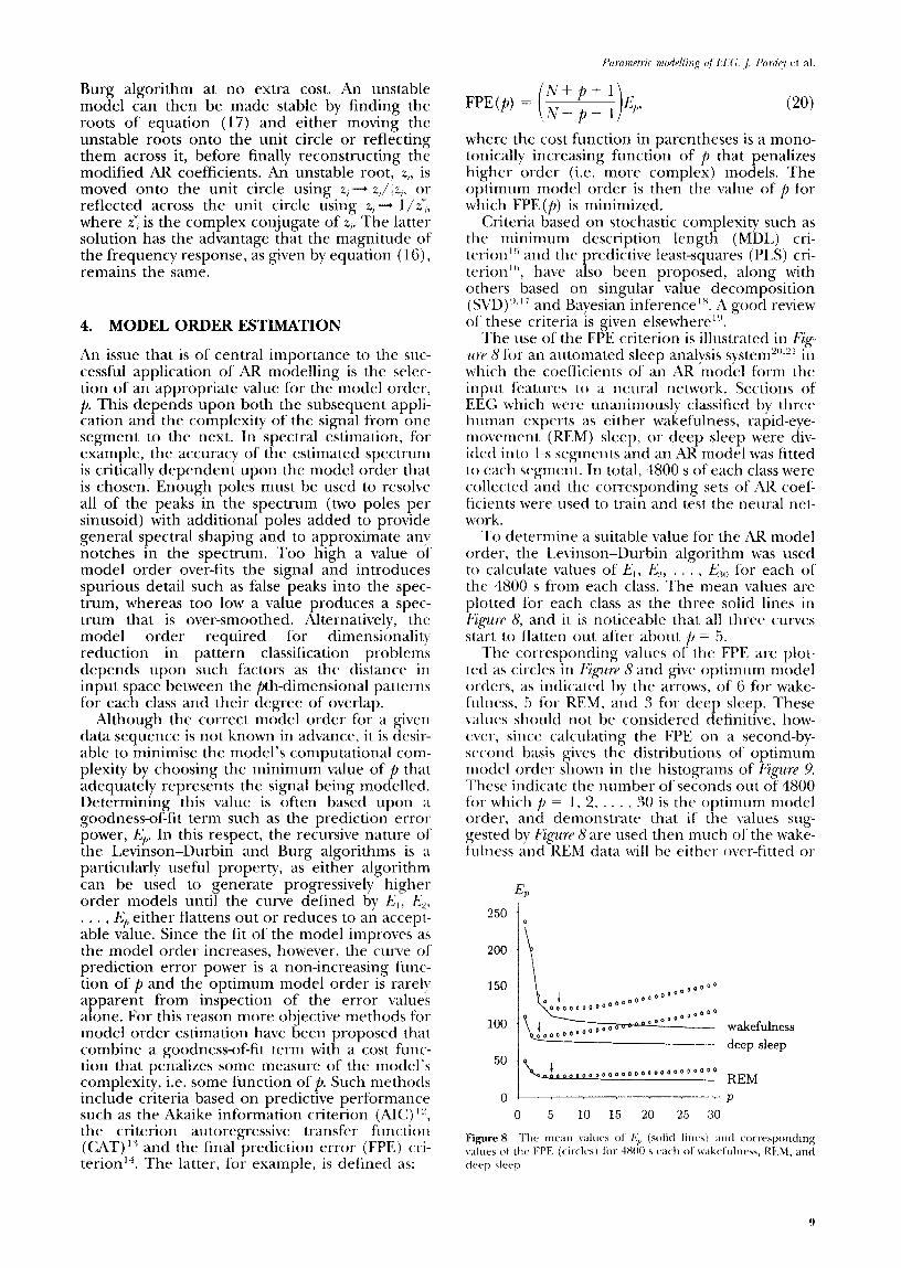
The use of the FPE criterion is illustrated in I;is- NW 8 for an automated sleep analysis system’“,g’ in which the coefficients of an AR model form the input features to a neural network. Sections of EEG which were unanimously classified by three human experts as either wakefulness, rapid-eye- movement (REM) sleep, or deep sleep were divided into l-s segments and an AR model was fitted to each segment. In total, 4800 s of each class were collected and the corresponding sets of AR coefficients were used to train and test the neural network.

To determine a suitable value for the AR model order, the Levinson-Durbin algorithm was used to calculate values of El, K2, . . . , b&, fi)r each of the 4800 s from each class. The mean values are plotted for each class as the three solid lines in Fi~gzm K, and it is noticeable that all three curves start to flatten out after about p = 5.

The corresponding values of the FPE are plotted as circles in Z@UW 8 and give optimum model orders, as indicated by the arrows, of 6 for wake- fillness, 5 for REM, and 3 for deep sleep. These values should not be considered definitive, however, since calculating the FPE on a second-by- second basis gives the distributions of optimum model order shown in the histograms of I;i~r~ 9. These indicate the number of seconds out kf 4800 fi)r which p = 1, 2. . . , 30 is the optimum model order, and demonstrate that if the values sug- gested by I;iguru 8 are used then much of’ the wake- fi’lness and REM data will he either o\,cr-fitted or

EP 250

200

150

100

50

0

Figure 8

Figure 9 The distribution of optimum model order on a second- by-second basis

under-fitted (this is not true of deep sleep, however, since its histogram is sharply peaked). It may thus be more appropriate to use those values that either optimally fit the most data-corresponding to the modes of the distributions in fipre 9-or over-fit as much data as they under-fit, corresponding to the medians of the distributions.

Figure 10 shows a human-scored hypnogram for a whole night’s sleep recording. This divides the recording into 30-s epochs and then assigns each epoch to one of seven classes using a set of standardized sleep-scoring ruleP. These classes correspond to wakefulness, movement (when the EEG is too corrupted to be reliably scored), REM, and four stages of progressively deeper sleep. The variation in optimum model order on a second-by- second basis is plotted below the hypnogram, and shows both the drop in model order associated with the initial descent from wakefulness into

hypnogram

Figure 10 The variation of optimum model order with sleep stage for a 7.5 h EEG recording

deep sleep, and the subsequent rise and fall in model order in phase with the regular modulation of REM and deep sleep.

The above example demonstrates the non-triv- ial nature of the model order selection problem. Moreover, since the number of inputs to a neural network must remain fixed, the model order used for feature extraction must also be fixed, regard- less of the non-stationarity of the EEG and of the associated variations in optimum model order with time. A compromise can be found, however, by choosing the value of p that minimizes a criterion appropriate for quantifying the neural network’s performance: for example, the classification error rate on a cross-validation data set.

5. DISCUSSION

The purpose of this review has been to provide an intuitive and usable introduction to the very popular technique of autoregressive modelling, and to locate this within the wider framework of parametric modelling techniques in general. The two most popular and well-established methods for AR parameter estimation are the autocorrelation method, in which the Yule-Walker equations are solved using the Levinson-Durbin algorithm, and the maximum entropy method, as implemented by the Burg algorithm. The corre- spondence between AR modelling and IIR filtering highlights the need to monitor the model’s stability, and also leads to an understanding of its use in spectral estimation. Indeed, the advantages of AR spectral estimation over the FFT are mani- fold, particularly when using the Burg algorithm and when analysing short data sequences demanded by non-stationary signals.

A variation on the Burg algorithm can be obtained by removing the constraint that the AR coefficients are updated using the Levinson recursion and minimizing the expression for the mean of the forward and backward prediction error powers in equation (12) with respect to all of the coefficients, uPr, uPZ, . . . , a

f rather than

just c+,. Algorithms which follow t 1s strategyN2”,24 tend to yield marginally better spectral estimates than the Burg algorithm, but their solutions are computationally more expensive and are not guaranteed to be algebraically stable.

To track non-stationarities in the signal on a time scale shorter than the segment size, consecutive segments can be made to overlap, typically by half their length. However, in such situations it is often better to use an adaptive model such as the Kalman filter,3 in which the values of the AR coefficients are updated on a sample-by-sample basis, with the update being proportional to the difference between the actual value of the current sample and its predicted value using the present set of coefficients. The advantage of adaptive modelling is that it can be applied to non-stationary signals without segmentation, although the disadvan- tages are that it is computationally more expensive than non-adaptive modelling. Adaptive models also produce more data than they consume (i.e. p coefficients per sample compared to p coef-

10

ficients per N samples for non-adaptive models) so that for some applications the sets of AR coefficients may need to be averaged.

ACKNOWLEDGEMENTS

This paper was written during the course of a research project funded by Oxford Instruments plc through the DTI TAPM LINK initiative. The authors would like to thank Dr Brendan Ruck and Dr Mark Holt at Oxford University for their valu- able comments on the draft of this paper.

REFERENCES

1.

2.

5.

3.

:i.

6.

7.

8.

9.

IO.

11.

12.

13.

14.

15.

16.

17.

Barlow JS. Methods of analysis of nonstationary EEGs, with emphasis on segmentation techniques: a compara- tive review. ,J Clin Nwrophysiol, 1985, Z(3): 267-304. Isaksson A. Wennberg A, Zetterberg I.H. Cotnputet analysis of EEG signals with parametric models. Pror

IlXlC, 1981, 69(4): 451-61. Skdgen DW. Estimation of running frequency spectra using a Kalman filter algorithm. ,I Riomrd b;:‘)tg. 1988. lO(3): 275-9. Makhoul J. 1,inear prediction: a tutorial review. f’roc 11&p;. 1975, 63(4): 561-80. Blinowska &J, Malinowski M. Non-linear and linear forecasting of the EEG time series. niol Cybf~tet. 1991, 66(2): I .59-65. Press WH, Tcukolsky SA, Vetterling WT, Flannery BP. Nu merid ReripQ.5 in C, 2 nd Edition. Cambridge Llniversitv Press. 1992. Andersen N. On the calculation of filter coefficienLs for maxitnttm t’rttropy spectral analysis. G~op/y 1973, 39(l): 69-7 2 Andersen N, (:otntttettts on the performance of tnaxitnum c,ntropy algorithms. Proc IlCklC. 1978, 66(11): 1581-2. <:adzow JA. Spectral estimation: an overdetermined rational model equation approach. Pror Il<lCi*15 1982,

70(9): 907-3:). Kay SM, Marple SI.. Spectrum analysis - a tnodern prr- spective. Proc IbZX, 1981, 69(11): 1380-1419. Harris CJ. On the use of windows for harmonic analvsis with the discrete Fottrier transform. Pror IL’%, lCk8,

66(l): 51-W. Akaike H. A new look at the statistical model identifi- cation. /l+X ‘l’rans Autom Contr, 1974, 19(6): 716-23. Parzen E. Some recent advances in time series tnodelling. IbXk Tram .Aulomal Contr, 1974, 19(6): 723-30. Akdikr H. Fitting autoregressions for prediction. Ann 1n.d

.Shli.s/ Math, 1969, 21: 243-7. Rissdnen J. Modelling by shortest data description. .~uIo~ malira. 1978. 14(5): 465-71. Rissanen ,J. A predictive least-squares principle. ljlfjA / Ma/h Ctontr In/or-m, 1986. 3: 21 l-22. Konstantinides I(. Threshold bounds in SVD and a new iterative algorithm for order selection in AR models. ILEE ‘/)-an s Sip& Prowsring. 199 1 . 39(5): 12 18-2 I

18.

19.

20.

21.

‘)L) . ..-.

23.

24.

Duric PM, Kay SM. Order selection of. autoregressive models. IlClZ Trnn.r. Si,qnnl Proces.cing 1992, 40(11): 2829-33. Dickie JR, Nandi AK. On the performance of’ AR model order selection methods. Proc Sewnth 1:‘uro Sipnl Pro-

crrsing ConJ; l<dinburgh, 1994, 185 l-1. Roberts S. Tdrassenko I.. New method of automated sleep quantification. MQ~ &+ Bid 1:‘ng ti (Tompul, 1992, 30(5): 509-li. Roberts S, Tdrassenko I,. A1ttalysis of the sleep EEG using a multilayer network with spatial organisation. IU’ Pro-

ceedingdC 1992, 139(6): 420-5. Rechtschaffen -4, kles A. .A Manual 01 Standardized 7’k

mindog?‘, ‘lkchniqurs and .kon’ng .$stem for .yleep S%ages o/

Humnn Su/+ct.c, Public Health Service, L1.S. (Government Printing Office. Washington D.(:., I%t(. Marple I.. A new autoregressive spectrum analysis algorithm. Il+ZX T,n71( Aroust Sf,~~rh Signnl l’rocc~~, 1980. 28(4):

441-.X. L%~ch TJ, Uavton RW. Time series modelling and maxitnum entropy. Phys I:‘nr~h & Plan int, 1976. 12: I F-N-200.

APPENDIX

Derivation of the recursive relationships between q,,, and b,,,

From equation (2) :

Q,, -4 = .A,, - - I$,, 5 I, I

= ,., 3- ‘c /I,,,.!,, , + (‘/‘/J,! ,

$1 i’ : = 5,s + - “ii’ I ,,‘,, / + qqh, i’ + s (I, I, I #,/ ,,.(,, (1 t I ,

/’ ’ ~ Q/, I, ,, + “/‘/A ),, ,i + c (I,,, I ,‘,’ ,,‘,, II

However:

I1

A review of parametric modelling techniques for EEG analysisnin/Courses/Seminar14a/ARmodels.pdf ·...

Documents

Transcript of A review of parametric modelling techniques for EEG analysisnin/Courses/Seminar14a/ARmodels.pdf ·...