A Review of Kernel Density Estimation with Applications to ...

Zambom and Dias-A Review of Kernel Density Estimation with Applications to Econometrics

20

A Review of Kernel Density Estimation with Applications to Econometrics

Adriano Z. Zambom and Ronaldo Dias

Universidade Estadual de Campinas and Universidade Estadual de Campinas

ABSTRACT

Nonparametric density estimation is of great importance when econometricians want to model the probabilistic or stochastic structure of a data set. This comprehensive review

summarizes the most important theoretical aspects of kernel density estimation and

provides an extensive description of classical and modern data analytic methods to compute the smoothing parameter. Throughout the text, several references can be found

to the most up-to-date and cut point research approaches in this area, while econometric

data sets are analyzed as examples. Lastly, we present SIZer, a new approach introduced

by Chaudhuri and Marron (2000), whose objective is to analyze the visible features representing important underlying structures for different bandwidths.

Key words: Nonparametric Density Estimation, SiZer, Plug-In Bandwidth Selectors, Cross- Validation, Smoothing Parameter.

JEL Classifications: C14

1. INTRODUCTION

The field of econometrics focuses on methods that address the probabilistic or stochastic

phenomena involving economic data. Modeling the underlying probabilistic structure of the

data, i.e., the uncertainty of the process, is a crucial task, for it can be used to describe the

mechanism from which the data was generated. Thus, econometricians have widely explored

density estimation, both the parametric and nonparametric approaches, to identify these

structures and then make inferences about the unknown “true models”. A parametric model

assumes that the density is known up to a finite number of parameters, while a nonparametric

model allows great flexibility in the possible form, usually assuming that it belongs to some

infinite collection of curves (differentiable with square integrable second derivatives for

example). The most used approach is kernel smoothing, which dates back to Rosenblatt

(1956) and Parzen (1962). The aim of this paper is to review the most import aspects of kernel

density estimation, both traditional approaches and modern ideas.

A large extent of econometric research concerning estimation of densities has shown that a

well estimated density can be extremely useful for applied purposes. An interesting

comprehensive review of kernel smoothing and its applications can be found in Bierens

(1987). Silverman (1986) and Scott (1992) discuss kernel density estimation thoroughly,

giving details about assumptions on the kernel weight, properties of the estimator such as bias

and variance, and discusses how to choose the smoothness of the estimate. The choice of the

smoothing parameter is a crucial issue in nonparametric estimation, and will be discussed in

detail in Section 4.

Adriano Z. Zambom, Universidade Estadual de Campinas (email: [email protected]).

Ronaldo Dias, Universidade Estadual de Campinas (email: [email protected]).

Acknowledgments: This paper was partially supported with grant 2012/10808-2 FA- PESP (Fundação de

Amparo à Pesquisa do Estado de São Paulo).

mailto:[email protected]

mailto:[email protected]

International Econometric Review (IER)

21

The remainder of this paper is as follows. In Section 2 we describe the most basic and

intuitive method of density estimation: the histogram. Then, in Section 3 we introduce kernel

density estimation and the properties of estimators of this type, followed by an overview of

old and new bandwidth selection approaches in Section 4. Finally, SiZer, a modern idea for

accessing features that represent important underlying structures through different levels of

smoothing, is introduced in Section 5.

2. THE HISTOGRAM

The grouping of data in the form of a frequency histogram is a classical methodology that is

intrinsic to the foundations of a variety of estimation procedures. Providing useful visual

information, it has served as a data presentation device, however, as a density estimation

method, it has played a fundamental role in nonparametric statistics.

Basically, the histogram is a step function defined by bin heights, which equal the proportion

of observations contained in each bin divided by the bin width. The construction of the

histogram is very intuitive, and to formally describe this construction, we will now introduce

some notation. Suppose we observe random variables X1,...,Xn i.i.d. from the distribution

function Fx, and that Fx is absolutely continuous with respect to a Lesbegue measure on .

Assume that x1,...,xn are the data points observed from a realization of the random variables

X1,...,Xn. Define the bins as Ij = [x0 + jh, x0 + ( j+1 )h) , j = 1,…,k , for a starting point x0. Note that

jI

j hfdxxfIXP )()()( (2.1)

where ξ ∈ Ij and the last equality follows from the mean value theorem for continuous

bounded functions. Intuitively, we can approximate the probability of X falling into the

interval Ij by the proportion of observations in Ij, i.e.,

n

IxIXP

ji

j

}{#)(

(2.2)

Using the approximation in (2.2) and the equation in (2.1), the density function f(x) can be

estimated by

n

i

ji

ji

h IxInhnh

Ixxf

1

)(1}{#

)(ˆ

for x ∈ Ij (2.3)

where

otherwise0

if1)(

j

ji

IxIxI

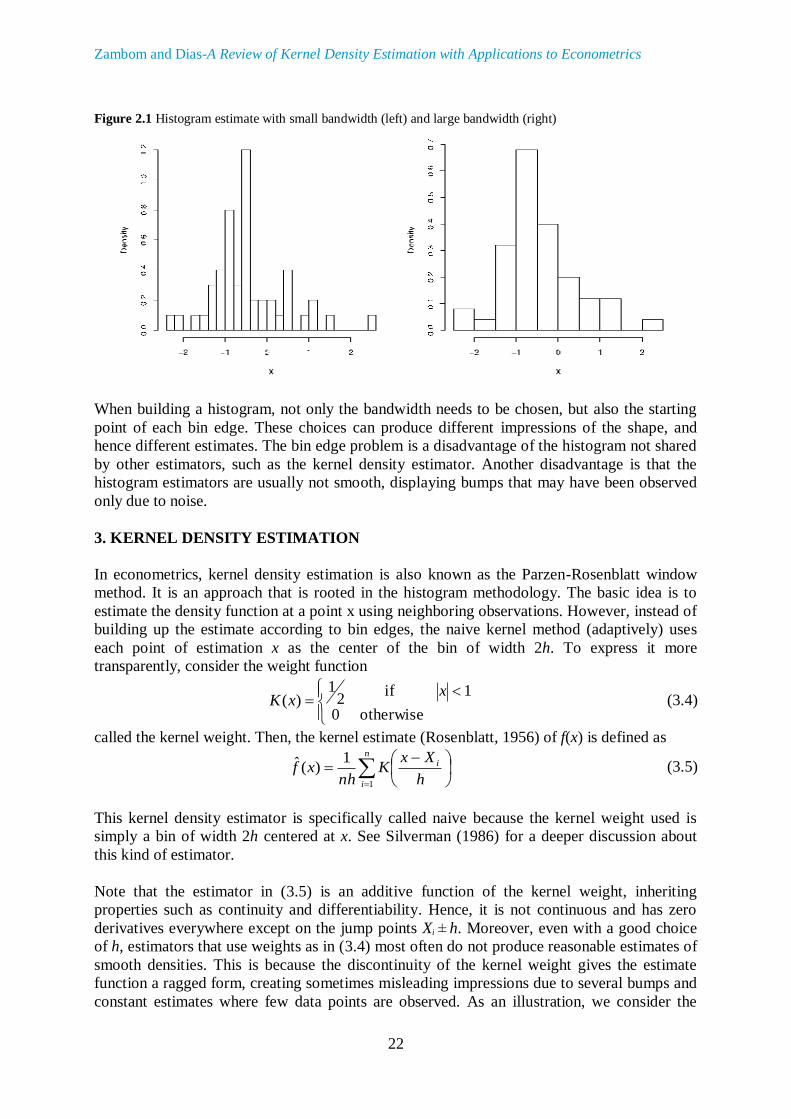
The smoothness of the histogram estimate is controlled by the smoothing parameter h, a

characteristic shared by all nonparametric curve estimators. Choosing a small bandwidth leads

to a jagged estimate, while larger bandwidths tend to produce over smoothed histogram

estimates (see Hardle, 1991). Figure 1 shows an example of two histograms of the same

randomly generated data: the histogram on the left hand side was estimated with a small

bandwidth and consequently has many bins, while the histogram on the right hand side was

computed with a large bandwidth, producing a smaller number of bins. The choice of the

bandwidth is discussed in more detail in Section 4. Note that in practice, the choice of k will

determine h or vice versa (a rule of thumb for the choice of k is the Sturges’ rule:

k·=·1·+·log2n·).


22

Figure 2.1 Histogram estimate with small bandwidth (left) and large bandwidth (right)

When building a histogram, not only the bandwidth needs to be chosen, but also the starting

point of each bin edge. These choices can produce different impressions of the shape, and

hence different estimates. The bin edge problem is a disadvantage of the histogram not shared

by other estimators, such as the kernel density estimator. Another disadvantage is that the

histogram estimators are usually not smooth, displaying bumps that may have been observed

only due to noise.

3. KERNEL DENSITY ESTIMATION

In econometrics, kernel density estimation is also known as the Parzen-Rosenblatt window

method. It is an approach that is rooted in the histogram methodology. The basic idea is to

estimate the density function at a point x using neighboring observations. However, instead of

building up the estimate according to bin edges, the naive kernel method (adaptively) uses

each point of estimation x as the center of the bin of width 2h. To express it more

transparently, consider the weight function

otherwise0

1if2

1)(

xxK (3.4)

called the kernel weight. Then, the kernel estimate (Rosenblatt, 1956) of f(x) is defined as

n

i

i

h

XxK

nhxf

1

1)(ˆ (3.5)

This kernel density estimator is specifically called naive because the kernel weight used is

simply a bin of width 2h centered at x. See Silverman (1986) for a deeper discussion about

this kind of estimator.

Note that the estimator in (3.5) is an additive function of the kernel weight, inheriting

properties such as continuity and differentiability. Hence, it is not continuous and has zero

derivatives everywhere except on the jump points Xi ± h. Moreover, even with a good choice

of h, estimators that use weights as in (3.4) most often do not produce reasonable estimates of

smooth densities. This is because the discontinuity of the kernel weight gives the estimate

function a ragged form, creating sometimes misleading impressions due to several bumps and

constant estimates where few data points are observed. As an illustration, we consider the


23

CEO compensation data in 2012, containing the 200 highest paid chief executives in the U.S.

This data set can be obtained from the Forbes website http://www.forbes.com/lists/2012

/12/ceo-compensation-12_rank.html.

For a better visualization of the plot, we excluded the number 1 in the ranking, with an

income of US$131.19 mil, as it was an outlier.

Figure 3.2 Estimated density of CEO compensation using the naive(solid line) and the Epanechnikov(dashed

line) kernels

Figure 3.2 shows two density estimators: the solid line represents the naive estimator, while

the dashed line represents a more adequate kernel type, called Epanechnikov, which will be

described later. The density estimated by the naive kernel appears to have several small

bumps, which are probably due to noise, not a characteristic of the true underlying density.

On the other hand, the Epanechnikov kernel is smooth, avoiding this issue.

Figure 3.3 Kernel weight functions

Kernel weight K(x)

Uniform )1|(|

2

1xI

Gaussian 2

21

2

1 xe

Epanechnikov )1|(|)1(

4

3 2 xIx

Biweight )1|(|)1(

16

15 22 xIx

Triweight )1|(|)1(

32

35 32 xIx

Table 3.1 : Kernel weight functions.

A usual choice for the kernel weight K is a function that satisfies ∫∞

–∞ K(x)dx = 1. If moreover, it

is assumed that K is a unimodal probability density function that is symmetric about 0, then

the estimated density f̂ (x) is guaranteed to be a density. Note that the weight in (3.4) is an

example of such choice. Suitable weight functions help overcome problems with bumps and

http://www.forbes.com/lists/2012%20/12/ceo-compensation-12_rank.html




24

discontinuity of the estimated density. For example, if K is a Gaussian distribution, the

estimated density function f̂ will be smooth and have derivatives of all orders. Table 3.1

presents some of the most used kernel functions and Figure 3.3 displays the format of the

Epanechnikov, Uniform, Gaussian and Triweight kernels.

One of the drawbacks of the kernel density estimation is that it is always biased, particularly

near the boundaries (when the data is bounded). However, the main drawback of this

approach happens when the underlying density has long tails. In this case, if the bandwidth is

small, spurious noise appears in the tail of the estimates, or if the bandwidth is large enough

to deal with the tails, important features of the main part in the distribution may be lost due to

the over-smoothing. To avoid this problem, adaptive bandwidth methods have been proposed,

where the size of the bandwidth depends on the location of the estimation. See Section 4 for

more details on bandwidth selection.

3.1. Properties of Kernel Density Estimators

In this section, some of the theoretical properties of the kernel density estimator are derived,

yielding reliable practical use. Assume we have X1,...,Xn i.i.d. random variables from a density

f and let K() be a Kernel weight function such that the following conditions hold

∫ K(u)du = 1, ∫ uK(u)du = 0, ∫ u2K(u)du = μ2(K) > 0

Then, for a non-random h, the expected value of f̂ (x) is

h

XxKE

hh

XxKE

nhxfE i

n

i

i 11))(ˆ(

1

(3.6)

dyyhxfyKduufh

uxK

n)()(

1

(3.7)

It is easy to see that f̂ is an asymptotic unbiased estimator of the density, since

E(f̂ (x))→·f(x)∫·K(y)dy = f(x) when h→0. It is important to note that the bandwidth strongly

depends on the sample size, so that when the sample size grows, the bandwidth tends to

shrink.

Now, assume also that the second derivative f” of the underlying density f is absolutely

continuous and square integrable. Then, expanding f (x+yh) in a Taylor series about x we have

)()(''2

1)(')()( 222 hoxfyhxhyfxfyhxf

Then, using the conditions imposed on the Kernel, the bias of the density estimator is

)()()(''2

))(ˆ( 2

2

2

hoKxfh

xfBias (3.8)

The variance of the estimated function can be calculated using steps similar to those in (3.6):

22 )))(ˆ((1

)(1

))(ˆ( xfEn

yhxfyKnh

xfVar

22 )}1()({1

)}1()({1

oxfn

dyoxfyKnh

)1

()(1 2

nhoxdyfyK

nh


25

)1

()()(1

nhoxfKR

nh

where R(g)=∫·g2(y)dy for any square integrable function g. From the definition of Mean

Square Error (MSE), we have

))(ˆ())(ˆ())()(ˆ())(ˆ( 22 xfBiasxfVardxxfxfxfMSE

)(1

)()(''4

)()(1 42

2

24

honh

oKxfh

xfKRnh

It is straightforward to see that, in order for the kernel density estimation to be consistent for

the underlying density, two conditions on the bandwidth are needed as n→∞: h→0 and

nh→∞. When these two conditions hold, MSE(f̂ (x))→0, and we have consistency. Moreover,

the trade-off between bias and variance is controlled by the MSE, where decreasing bias leads

to a very noise (large variance) estimate and decreasing variance yields over-smoothed

estimates (large bias). As has already been pointed out, the smoothness of the estimate

depends on the smoothing parameter h, which is chosen as a function of n. For the optimal

asymptotic choice of h, a closed form expression can be obtained from minimizing the Mean

Integrated Square Error (MISE). Integrating the MSE over the entire line, we find (Parzen,

1962)

4

)''()()())()(ˆ()ˆ(

2

2

42 fRKh

nh

KRdxxfxfEfMISE

(3.9)

and the bandwidth h that minimizes MISE is then

51

51

2

2 )''()(

)(

n

fRK

KRhMISE

(3.10)

Using this optimal bandwidth, we have

54

51

42

20 )''()()(4

5)ˆ(inf

nfRKRKfMISEh (3.11)

A natural question is how to choose the kernel function K to minimize (3.11). Interestingly, if

we restrict the choice to a proper density function, the minimizer is the Epanechnikov kernel,

where μ2

2(K)R4(K)=3

4/5

6.

The problem with using the optimal bandwidth is that it depends on the unknown quantity f”,

which measures the speed of fluctuations in the density f, i.e., the roughness of f. Many

methods have been proposed to select a bandwidth that leads to good performance in the

estimation, some of these are discussed in Section 4.

The asymptotic convergence of the kernel density estimator has been widely explored. Bickel

and Rosenblatt (1973) showed that for sufficiently smooth f and K,

)(/|)()(ˆ|sup xfxfxfI , when normalized properly, has an extreme value limit

distribution. The strong uniform convergence of f̂ (x)

0|)()(ˆ|suplim xfxfxn a.e. (3.12)

has been studied extensively when the observations are independent or weakly dependent.

Nadaraya (1965) showed that if K is of bounded variation and if f is uniformly continuous,


26

then (3.12) holds as long as 1

2

m

mhne

for each γ > 0. Moreover, Stute (1982) derives a

law of the logarithm for the maximal deviation between a kernel density estimator and the

true underlying density function, Gine and Guillou (2002) find rates for the strong uniform

consistency of kernel density estimators and Einmahl and Mason (2005) introduce a general

method to prove uniform in bandwidth consistency of kernel-type function estimators. Other

results on strong uniform convergence with different conditions can be found in several other

papers, such as Parzen (1962), Bhattacharya (1967), Van Ryzin (1969), Moore and Yackel

(1977), Silverman (1978) and Devroye and Wagner (1980).

4. THE CHOICE OF THE SMOOTHING PARAMETER h

Selecting an appropriate bandwidth for a kernel density estimator is of crucial importance,

and the purpose of the estimation may be an influential factor in the selection method. In

many situations, it is sufficient to subjectively choose the smoothing parameter by looking at

the density estimates produced by a range of bandwidths. One can start with a large

bandwidth, and decrease the amount of smoothing until reaching a “reasonable” density

estimate. However, there are situations where several estimations are needed, and such an

approach is impractical. An automatic procedure is essential when a large number of

estimations are required as part of a more global analysis.

The problem of selecting the smoothing parameter for kernel estimation has been explored by

many authors, and no procedure has yet been considered the best in every situation.

Automatic bandwidth selection methods can basically be divided in two categories: classical

and plug-in. Plug-in methods refer to those that find a pilot estimate of f, sometimes using a

pilot estimate of h, and ”plug it in” the estimation of MISE, computing the optimal bandwidth

as in (3.10). Classical methods, such as cross-validation, Mallow’s Cp, AIC, etc, are basically

extensions of methods used in parametric modeling. Loader (1999) discusses the advantages

and disadvantages of the plug-in and classical methods in more detail. Besides these two

approaches, it is possible to find an estimate of h based on a reference density. Next, we

present in more detail the reference method and the most used automatic bandwidth selection

procedures.

4.1. Reference to a Distribution

A natural way to overcome the problem of not knowing f” is to choose a reference density for

f, compute f” and substitute it in (3.10). For example, assume that the reference density is

Gaussian, and a Gaussian kernel is used, then

51

51

521

1

51

51

2

2

06.1

83

2

)''()(

)(

nnn

fRK

KRhMISE

By using an estimate of σ, one has a data-based estimate of the optimal bandwidth. In order to

have an estimator that is more robust against outliers, the interquartile range R can be used as

a measure of the spread. This modified version can be written as

51

34.1

ˆ,ˆmin06.1ˆ

n

Rhrobust


27

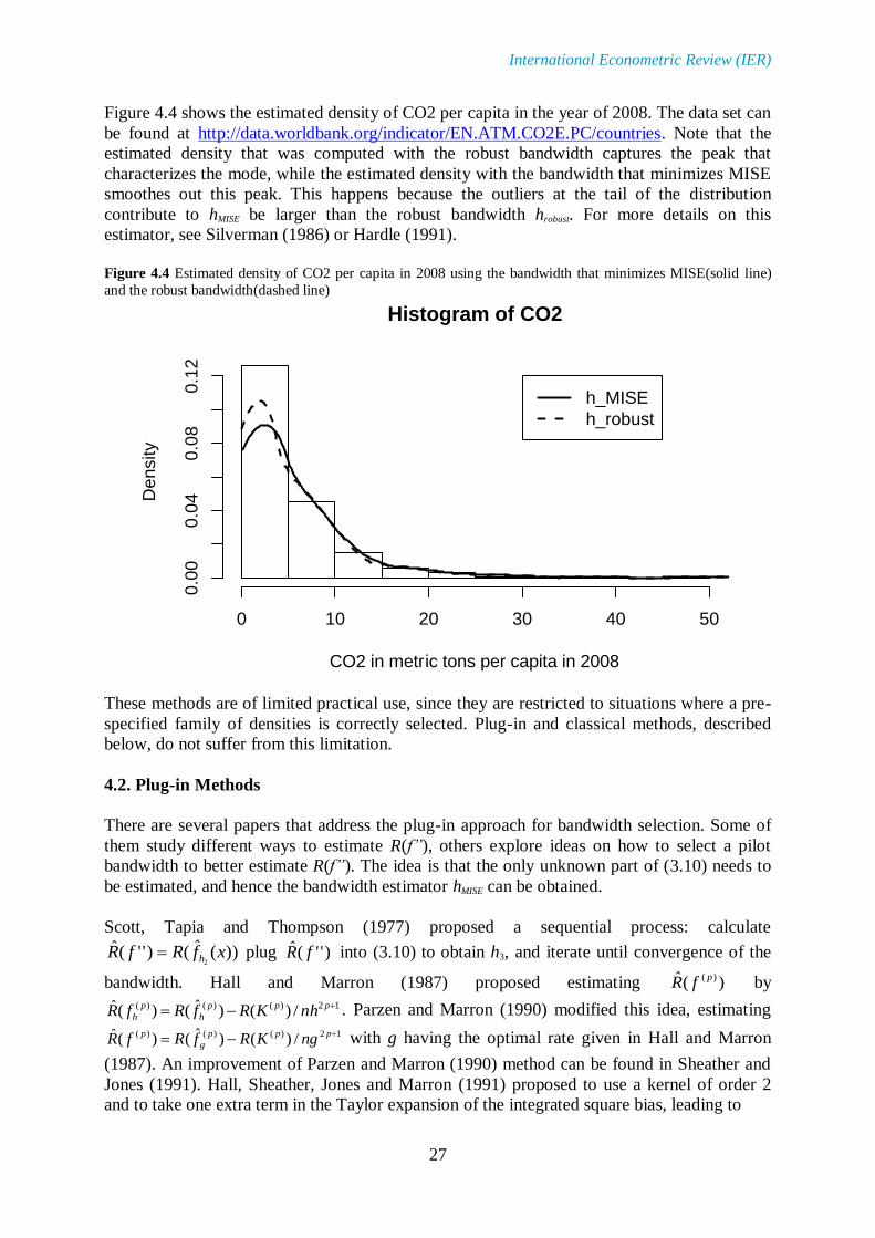
Figure 4.4 shows the estimated density of CO2 per capita in the year of 2008. The data set can

be found at http://data.worldbank.org/indicator/EN.ATM.CO2E.PC/countries. Note that the

estimated density that was computed with the robust bandwidth captures the peak that

characterizes the mode, while the estimated density with the bandwidth that minimizes MISE

smoothes out this peak. This happens because the outliers at the tail of the distribution

contribute to hMISE be larger than the robust bandwidth hrobust. For more details on this

estimator, see Silverman (1986) or Hardle (1991).

Figure 4.4 Estimated density of CO2 per capita in 2008 using the bandwidth that minimizes MISE(solid line)

and the robust bandwidth(dashed line)

These methods are of limited practical use, since they are restricted to situations where a pre-

specified family of densities is correctly selected. Plug-in and classical methods, described

below, do not suffer from this limitation.

4.2. Plug-in Methods

There are several papers that address the plug-in approach for bandwidth selection. Some of

them study different ways to estimate R(f”), others explore ideas on how to select a pilot

bandwidth to better estimate R(f”). The idea is that the only unknown part of (3.10) needs to

be estimated, and hence the bandwidth estimator hMISE can be obtained.

Scott, Tapia and Thompson (1977) proposed a sequential process: calculate

))(ˆ()''(ˆ2

xfRfR h plug )''(ˆ fR into (3.10) to obtain h3, and iterate until convergence of the

bandwidth. Hall and Marron (1987) proposed estimating )(ˆ )( pfR by

12)()()( /)()ˆ()(ˆ ppp

h

p

h nhKRfRfR . Parzen and Marron (1990) modified this idea, estimating

12)()()( /)()ˆ()(ˆ ppp

g

p ngKRfRfR with g having the optimal rate given in Hall and Marron

(1987). An improvement of Parzen and Marron (1990) method can be found in Sheather and

Jones (1991). Hall, Sheather, Jones and Marron (1991) proposed to use a kernel of order 2

and to take one extra term in the Taylor expansion of the integrated square bias, leading to

Histogram of CO2

CO2 in metric tons per capita in 2008

De

nsity

0 10 20 30 40 50

0.0

00.0

40

.08

0.1

2

h_MISE

h_robust

http://data.worldbank.org/indicator/EN.ATM.CO2E.PC/countries


28

)''()()(24

)()( 42

4

2 fRKKh

nh

KRhMISE (4.13)

Since the minimizer of (4.13) is not analytically feasible, they proposed to estimate the

bandwidth by

53

12

51

1 /ˆˆ/ˆ nJJnJhHSIM

where )''(ˆ)(

)(ˆ2

2

1fRK

KRJ

, and

)''(ˆ)(20

)''(ˆ)(ˆ

2

42

fRK

fRKJ

.

Several other plug-in methods have been proposed, and a review of the first procedures that

address this type of methodology can be found in Turlach (1993). Modern research on plug-in

methods have actually become somewhat hybrid, combining ideas of plug-in and classical

approaches such as cross validation, see Biased Cross-Validation described below for

example. More recently, inspired by developments in threshold selection, Chan, Lee and Peng

(2010) propose to choose h = o(n-1/5

) as large as possible, so that the density estimator has a

larger bias, but smaller variance than )(ˆ xfAMSEh . The idea is to consider an alternative kernel

density estimator

n

i

i

h

XxK

nhf

1

1, and define

2/1

22/1 ))()(();(ˆ

);();(ˆ);(

dssKsKhxf

hxfhxfnhhxn .

Then, the choice for the smoothing parameter is

][, allfor |);(:|minargˆ ,5/1

n

nI cnrhrzrxhh .

where zα denotes a critical point in N(0,1), c > 0 and 0 < ε < 1/5 . The intuition is that, when h is

large zrxn );( , since )1,0();( Nrxd

n .

4.3. Classical Methods

4.3.1. Least Squares Cross-Validation

Cross-validation is a popular and readily implemented heuristic for selecting the smoothing

parameter in kernel estimation. Introduced by Rudemo (1982) and Bowman (1984), least

squares cross-validation is very intuitive and has been a fundamental device in recent

research. The idea is to consider the expansion of the Integrated Square Error (ISE) in the

following way

dxxfdxxfxfdxxfhISE hh )()()(ˆ)(ˆ)( 22.

Note that the last term does not depend on f̂ h, hence on h, so that we only need to consider the

first two terms. The ideal choice of bandwidth is the one which minimizes

dxxfxfdxxfdxxfhISEhL hh )()(ˆ)(ˆ)()()( 22

The principle of the least squares cross-validation method is to find an estimate of L(h) from

the data and minimize it over h. Consider the estimator


29

i

iihhLS Xfn

dxxfhCV )(ˆ12)(ˆ)( 2

,

2 (4.14)

where

ij

j

iihh

XxK

hnXf

)1(

1)(ˆ

, (4.15)

The summation in (4.14) has expectation

dxxfxfEdxxfxfEXfEXfn

E hnh

i

nnhiih )()(ˆ)()(ˆ)(ˆ)(ˆ1,,,

because E(f̂ h) depends only on the kernel and bandwidth, not on the sample size. It follows

that E(CVLS(h)) = E(L(h)) and hence CVLS(h) + ∫ f 2(x)dx is an unbiased estimator of MISE

(reason why this method is also called unbiased cross-validation). Assuming that the

minimizer of CVLS(h) is close to the minimizer of E(CVLS(h)), the bandwidth

)(minarg hCVh LShLSCV

is the natural choice. This method suffers from sample variation, that is, using different

samples from the same distribution, the estimated bandwidths may have large variance.

Further discussion on this method can be found in Bowman, Hall and Titterington (1984),

Hall (1983) and Stone (1984).

4.3.2. Biased Cross-Validation

Biased cross-validation considers the asymptotic MISE

)''()(4

)(}ˆ{ 2

2

4

fRKh

nh

KRfAMISE h

This method was suggested by Scott and Terrell (1987), and its main idea is to replace the

unknown quantity R(f′′) by the estimator

)''()()''ˆ()''(~ 15 KRnhfRfR h

ji

jihh XXKKn ))(""*(2

to give

)''(~

)(4

)()( 2

2

4

fRKh

nh

KRhBCV

Then, the bandwidth selected is hBCV = argmin BCV(h). This selector is considered a hybrid of

cross-validation and plug-in, since it replaces an unknown value in AMISE by a cross-

validation kernel estimate )''(~

fR .

4.3.3. Likelihood Cross-Validation

Suppose that in addition to the original data set X1,...,Xn, we have another independent

observation X* from f. Thinking of on f̂ h, as a parametric family depending on h, but with

fixed data X1,...,Xn, we can view log f̂ (X*) as the likelihood of the bandwidth h. Because in

reality no additional observation is available, we can omit a randomly selected observation

from the original data, say Xi, and compute )(ˆ, iih Xf , as in (4.15). Note that there is no


30

pattern when choosing the observation to be omitted, so that the score function can be taken

as the log likelihood average

n

i

iih XfnhCV1

,

1 )(ˆlog)(

Naturally, we choose the bandwidth the minimizes CV(h), which is known to minimize the

Kullback-Leibler distance between )(ˆ xfh and f(x). This method was proposed by Habbema,

Hermans and van den Broek (1974) and Duin (1976), but other results can be found in

Marron (1987), Marron (1989) and Cao, Cuevas and Gonzalez-Manteiga (1994).

In general, bandwidths chosen via cross validation methods in kernel density estimation are

highly variable, and usually give undersmooth density estimates, causing undesired spurious

bumpiness.

4.3.3. Likelihood Cross-Validation

The Indirect Cross-validation (ICV) method, proposed by Savchuk, Hart and Sheather (2010),

slightly outperforms least squares cross-validation in terms of mean integrated squared error.

The method can be described as follows. First define the family of kernels

}0,0:),(.;{ LL where, for all u, )()()1(),;(

uuuL .

Note that this is a linear combination of two Gaussian kernels. Then, select the bandwidth of

an L-kernel estimator using least squares cross-validation, and call it UCVb̂ . Under some

regularity conditions on the underlying density f, hn and bn that asymptotically minimize the

MISE of φ and L-kernel estimators, have the following relation

nnn Cbb

LR

LRh

5/1

2

2

2

2

)()(

)()(

.

The indirect cross-validation bandwidth is chosen to be UCVICV bCh ˆˆ . Savchuk et al. (2010)

show that the relative error of ICV bandwidths can converge to 0 at a rate of n1/4

, much better

than the n1/10

rate of LSCV.

4.4. Other Methods

4.4.1. Variable Bandwidth

Rather than using a single smoothing parameter h, some authors have considered the

possibility of using a bandwidth h(x) that varies according to the point x at which f is

estimated. This is often referred as the balloon estimator and has the form

n

i

i

xh

XxK

xnhxf

1 )()(

1)(ˆ (4.16)

The balloon estimator was introduced by Loftsgaarden and Quesenberry (1965) in the form of

the k-th nearest neighbor estimator. In Loftsgaarden and Quesenberry (1965), h(x) was based

on a suitable number k, so that it was a measure of the distance between x and the k-th data


31

point nearest to x. The optimal bandwidth for this case can be shown to be (analogue of, 3.10,

for asymptotic MSE)

51

51

22

2 )('')(

)()()(

n

xfK

xfKRxhAMSE

(4.17)

Another variable bandwidth method is to have the bandwidth vary not with the point of

estimation, but with each observed data point. This type of estimator, known as sample point

or variable kernel density estimator, was introduced by Breiman et al. (1977) and has the form

n

i i

i

i Xh

XxK

Xnhxf

1 )()(

1)(ˆ (4.18)

This type of estimator has one advantage over the balloon estimator: it will always integrate

to 1, assuring that it is a density. Note that h(Xi) is a function of random variables, and thus it

is also random.

More results on the variable bandwidth approach can be found in Hall (1992), Taron et al.

(2005), Wu et al. (2007) and Gine and Sang (2010).

4.4.2. Binning

An adaptive type of procedure is the binned kernel density estimation, studied by a few

authors such as Scott (1981), Silverman (1982) and Jones (1989). The idea is to consider

equally spaced bins Bi with centers at ti and bin counts ni, and define the estimator as

m

i

i

i

iibin

h

txK

nh

txKn

nxf

1

11)(ˆ (4.19)

where the sum over m means summing over the finite non-empty bins that exist in practice. It

is also possible to use a variable bandwidth in (4.19), yielding the estimator

m

i i

ibin

Xh

txK

nxf

1 )(

1)(

~ (4.20)

Examples of other approaches and discussion on this type of estimation can be found in Hall

and Wand (1996), Cheng (1997), Minnotte (1999), Pawlak and Stadtmuller (1999),

Holmstrom (2000).

4.4.3. Bootstrap

A methodology that has been recently explored is that of selecting the bandwidth using

bootstrap. It focuses on replacing the MSE by MSE*, a bootstrapped version of MSE, which

can be minimized directly. Some authors resample from a subsample of the data X1,...,Xn (see

Hall, 1990), others replace from a pilot density based on the data (see Faraway and Jhun,

1990; Hazelton, 1996; Hazelton, 1999), more precisely, from

n

i n

i

n

b

hb

XxL

nbxf

1

1)(

~

where L is another kernel and bn is a pilot bandwidth. Since the bandwidth choice reduces to

estimating s in h = n–1/5

s, Ziegler (2006) introduces


32

n

i

isn

sn

XxK

snxf

15/1

*

5/4

*

,

1)(

and obtain )))(~

)((()( 2*

,

**

, xfxfExMSE b

hsnsn . The proposed bandwidth is

*

,

5/1 minarg snsn MSEnh

Applications of the bootstrap idea can be found in many different areas of estimation, see

Delaigle and Gijbels (2004), Loh and Jang (2010) for example.

4.4.4. Estimating Densities on +

It is known that kernel density estimators have larger bias on the boundaries. Many methods

have been proposed to alleviate such problem, such as the use of gamma kernels or inverse

and reciprocal inverse Gaussian kernels, also known as varying kernel approach. Chen (2000)

proposes to replace the symmetric kernel by a gamma kernel, which has flexible shapes and

locations on +. Their estimator can be described in the following way. Suppose the

underlying density f has support [0, ∞) and consider the gamma kernel

)1/(

)(1/

//

,1/

bxb

ettK

bx

btbx

bbx

where b is a smoothing parameter such that b® 0 and nb®¥. Then, the gamma kernel

estimator is defined as

n

i

ibbx

G XKn

xf1

,1/ )(1

)(ˆ

The expected value of this estimator is

)()()()(ˆ

0

,1/ xbbx

G EfdyyfyKxfE

where ξx is a Gamma(x/b+1,b) random variable. Using Taylor Expansion and the fact that

E(ξx) = x + b and Var(ξx)= xb + b2 we have that

)()()(''2

1)()( boVarxfbxfEf xx

)()](''2

1)('[)( boxxfxfbxf

It is clear then, that this estimator does not have bias problems on the boundaries, since the

bias is o(b) near the origin and in the interior. See Chen (2000) for further details. Other

approaches on estimating the density on can be found in Scaillet (2004), Mnatsakanov

and Ruymgaart (2012), Mnatsakanov and Sarkisian (2012), Comte and V.Genon-Catalot

(2012) and references therein.

Some interest on density estimation research is on bias reduction techniques, which can be

found in Jones, Linton and Nielsen (1995), Choi and Hall (1999), Cheng et al. (2000), Choi et

al.(2000) and Hall and Minnotte (2002). Other recent improvements and interesting

applications of the kernel estimate can be found in Hirukawa (2010), Liao et al. (2010),

Matuszyk et al. (2010), Miao et al. (2012), Chu et al. (2012), Golyandina et al. (2012) and Cai

et al. (2012) among many others.

Â+


33

4.4.5. Estimating the distribution function F(x)

It is not uncommon to find situations where it is desirable to estimate the distribution function

F(x) instead of the density function f(x). A whole methodology known as kernel distribution

function estimation (KDFE) has been explored since Nadaraya (1964) introduced the

estimator

n

i

in

h

XxK

nxF

1

1)(ˆ

where K is the distribution function of a positive kernel k, i.e, K(x) = ∫x

–∞ k(t)dt. Authors have

considered many alternatives for this estimation, but the basic measures of quality or this type

of estimator are

)()()]()(ˆ[)( 2 xdFxWxFxFhISE h and

)()()]()(ˆ[)( 2 xdFxWxFxFEhMISE h

where W is a non-negative weight function.

Sarda (1993) considered a discrete approximation to MISE, the average squared error

n

i

iiih XWXFXFn

hASE1

2 )()]()(ˆ[1

)(

He suggests replacing the unknown F(Xi) by the empirical Fh(Xi) and then selecting the

bandwidth that minimizes the leave-one-out criterion

n

i

iiniih XWXFXFn

hCV1

2

, )()]()(ˆ[1

)(

As an alternative to this cross-validation criterion, Altman and Leger (1995) introduce a plug-

in estimator of the asymptotically optimal bandwidth. There is a vast literature on estimating

kernel distribution functions, for example Bowman, Hall and Prvan (1998), Tenreiro (2006),

Ahmad and Amezziane (2007), Janssen et al. (2007), Berg and Politis (2009), just to cite a

few.

4.5. Example of Bandwidth Selection Methods

It is well known that plug-in bandwidth estimators tend to select larger bandwidths when

compared to the classical estimators. They are usually tuned by arbitrary specification of pilot

estimates and most often produce over smoothed results when the smoothing problem is

difficult. On the other hand, smaller bandwidths tend to be selected by classical methods,

producing under smoothed results. The goal of a selector of the smoothing parameter is to

make that decision purely from the data, finding automatically which features are important

and which should be smoothed away.

Figure 4.5 shows an example of classical and plug-in bandwidth selectors for a real data set.

The data corresponds to the exports of goods and services of countries in 2011, representing

the value of all goods and other market services provided to the rest of the world. The data set

can be downloaded from the world bank website (http://data.worldbank.org).

http://data.worldbank.org/


34

Figure 4.5 Estimated densities for bandwidths chosen using different methods

The plug-in estimators a) rule of thumb for Gaussian and b) Seather and Jones selector

produced a very smooth fit, while unbiased cross-validation selects a small bandwidth,

yielding a highly variable density estimate. The hybrid method biased cross-validation, is the

one that selects the largest bandwidth, hence its corresponding density estimate is very

smooth, smoothing away information of the peak (mode).

5. SiZer

In nonparametric estimation, the challenge of selecting the smoothing parameter that yields

the best possible fit has been addressed through several methods, as described in previous

sections. The challenge is to identify the features that are really there, but at the same time to

avoid spurious noise. Marron and Chung (1997) and other authors noted that it may be worth

to consider a family of smooths with a broad range of bandwidths, instead of a single

estimated function. Figure 5.6 shows an example of a density generated from a mixture of a

Gaussian variable with mean 0 and variance 1 and another Gaussian variable, with mean 8

and variance 2. The density was estimated with a Epanechnikov kernel using bandwidths that

vary from 0.4 to 10. The wide range of smoothing considered, from a small bandwidth

producing a wiggly estimate to a very large bandwidth yielding nearly the simple least

squares fit, allows a contrast of estimated features at each level of smoothing. The two

highlighted bandwidths are equal to 0.6209704 and 1.493644, corresponding to the choice of

biased cross-validation (blue) and to Silverman’s rule of thumb (red) (see Silverman, 1986)

respectively.

The idea of considering a family of smooths has its origins in scale space theory in computer

science. A fundamental concept in such analysis is that it does not aim at estimating one true

curve, but at recovering the significant aspects of the underlying function, since different

levels of smoothing may reveal different intrinsic features. Exploring this concept in a

statistical point of view, Chaudhuri and Marron (2000) introduced a procedure called

SIignificance ZERo crossings of smoothed estimates (SiZer), whose objective is to analyze

the visible features representing important underlying structures for different bandwidths.

Next, we briefly describe such method.

Suppose that h ∈ H, where H is a subinterval of (0,∞), and x ∈ I, where I is a subinterval of

(−∞, ∞). Then the family of smooth curves { )(ˆ xfh | h ∈ H, x ∈ I} can be represented by a

surface called scale space surface, which captures different structures of the curve under


35

different levels of smoothing. Hence, the focus is really on ))(ˆ( XfE h as h varies in H and x

in I, which is called in Chaudhuri and Marron (2000) as ”true curves viewed at different

scales of resolution”.

Figure 5.6 Estimated density with several bandwidths

A smooth curve )(ˆ xfh has derivatives equal to 0 at points of minimum (valleys), maximum

(peaks) and points of inflection. Note that, before a peak (or valley), the sign of the derivative

xxf h /)(ˆ is positive (or negative), and after it the derivative is negative (or positive). In

other words, peaks and valleys are determined by zero crossings of the derivative. Actually,

we can identify structures in a smooth curve by zero crossings of the m-th order of the

derivative. Using a Gaussian kernel )2/exp()2/1()( 2xxK , Silverman (1981) showed

that the number of peaks in a kernel density estimate decreases monotonically with the

increase of the bandwidth, and Chaudhuri and Marron (2000) extended this idea for the

number of zero crossings of the m-th order derivative m

h

m xxf /)(ˆ in kernel regression.

The asymptotic theory of the scale space surfaces and their derivatives studied by Chaudhuri

and Marron (2000), which hold even under bootstrapped or resampled distributions, provides

tools for building bootstrap confidence intervals and tests of significance for their features

(see Chaudhuri and Marron, 1999). SiZer basically considers the null hypothesis

0/))(ˆ(:,

0 m

h

mxh xxfEH

for a fixed x ∈ I and h ∈ H. If xhH ,

0 is rejected, there is evidence that m

h

m xxfE /))(ˆ( positive

or negative, according to the sign of m

h

m xxf /)(ˆ .

The information is displayed in a color map of scale space, where the pixels represent the

X

0

5

10

h

2

4

6

8

10

0.05

0.10

0.15

0.20

0.25

Mixture of Normals Density


36

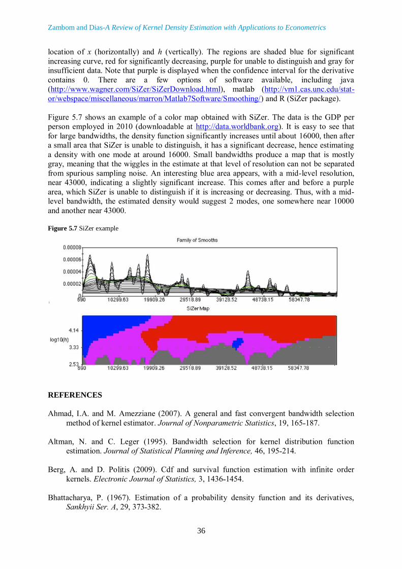
location of x (horizontally) and h (vertically). The regions are shaded blue for significant

increasing curve, red for significantly decreasing, purple for unable to distinguish and gray for

insufficient data. Note that purple is displayed when the confidence interval for the derivative

contains 0. There are a few options of software available, including java

(http://www.wagner.com/SiZer/SiZerDownload.html), matlab (http://vm1.cas.unc.edu/stat-

or/webspace/miscellaneous/marron/Matlab7Software/Smoothing/) and R (SiZer package).

Figure 5.7 shows an example of a color map obtained with SiZer. The data is the GDP per

person employed in 2010 (downloadable at http://data.worldbank.org). It is easy to see that

for large bandwidths, the density function significantly increases until about 16000, then after

a small area that SiZer is unable to distinguish, it has a significant decrease, hence estimating

a density with one mode at around 16000. Small bandwidths produce a map that is mostly

gray, meaning that the wiggles in the estimate at that level of resolution can not be separated

from spurious sampling noise. An interesting blue area appears, with a mid-level resolution,

near 43000, indicating a slightly significant increase. This comes after and before a purple

area, which SiZer is unable to distinguish if it is increasing or decreasing. Thus, with a mid-

level bandwidth, the estimated density would suggest 2 modes, one somewhere near 10000

and another near 43000.

Figure 5.7 SiZer example

REFERENCES

Ahmad, I.A. and M. Amezziane (2007). A general and fast convergent bandwidth selection

method of kernel estimator. Journal of Nonparametric Statistics, 19, 165˗187.

Altman, N. and C. Leger (1995). Bandwidth selection for kernel distribution function

estimation. Journal of Statistical Planning and Inference, 46, 195˗214.

Berg, A. and D. Politis (2009). Cdf and survival function estimation with infinite order

kernels. Electronic Journal of Statistics, 3, 1436˗1454.

Bhattacharya, P. (1967). Estimation of a probability density function and its derivatives,

Sankhyii Ser. A, 29, 373˗382.

http://www.wagner.com/SiZer/SiZerDownload.html

http://vm1.cas.unc.edu/stat-or/webspace/miscellaneous/marron/Matlab7Software/Smoothing/

http://vm1.cas.unc.edu/stat-or/webspace/miscellaneous/marron/Matlab7Software/Smoothing/

http://data.worldbank.org/


37

Bickel, P. J. and M. Rosenblatt (1973). On some global measures of the deviations of density

function estimates. The Annals of Statistics, 1071˗1095.

Bierens, H.J. (1987). Kernel estimators of regression functions. In Advances in Econometrics:

Fifth World Congress, Vol.I, Cambridge University Press 99˗144.

Bowman, A.W. (1984). An alternative method of cross-validation for the smoothing of

density estimates. Biometrika, 71, 353˗360.

Bowman, A.W., P. Hall and T. Prvan (1998). Bandwidth selection for the smoothing of

distribution function. Biometrika, 85, 799˗808.

Bowman, A.W., P. Hall and D.M. Titterington (1984). Cross-validation in nonparametric

estimation of probabilities and probability densities. Biometrika, 71, 341˗351.

Breiman, L., W. Meisel and E. Purcell (1977). Variable kernel estimates of multivariate

densities. Technometrics, 19, 135˗144.

Cai, Q., G. Rushton, and B. Bhaduri (2012). Validation tests of an improved kernel density

estimation method for identifying disease clusters. Journal of Geographical Systems, 14

(3), 243˗264.

Cao, R., A. Cuevas and W. Gonzalez-Manteiga (1994). A comparative study of several

smoothing methods in density estimation. Computational Statistics & Data Analysis, 17

(2), 153˗176.

Chan, N.-H., T.C. Lee and L. Peng (2010). On nonparametric local inference for density

estimation. Computational Statistics & Data Analysis, 54, 509˗515.

Chaudhuri, P. and J.S. Marron (1999). Sizer for exploration of structures in curves. Journal of

the American Statistical Association, 94, 807˗823.

Chaudhuri, P. and J.S. Marron (2000). Scale space view of curve estimation. The Annals of

Statistics, 28, 402˗428.

Chen, S. (2000). Probability density function estimation using gamma kernels. Annals of the

Institute of Statistical Mathematics, 52, 471˗480.

Cheng, M.-Y. (1997). A bandwidth selector for local linear density estimators. The Annals of

Statistics, 25, 1001˗1013.

Cheng, M.-Y., E. Choi, J. Fan and P. Hall (2000). Skewing-methods for two parameter

locally-parametric density estimation. Bernoulli, 6, 169˗182.

Choi, E. and P. Hall (1999). Data sharpening as prelude to density estimation. Biometrika, 86,

941˗947.

Choi, E., P. Hall and V. Roussan (2000). Data sharpening methods for bias reduction in

nonparametric regression. Annals of Statistics, 28, 1339˗1355.


38

Chu, H.-J., C.-J. Liau, C.-H. Lin and B.-S. Su (2012). Integration of fuzzy cluster analysis and

kernel density estimation for tracking typhoon trajectories in the Taiwan region. Expert

Systems with Applications, 39, 9451˗9457.

Comte, F. and V. Genon-Catalot (2012). Convolution power kernels for density estimation.

Journal of Statistical Planning and Inference, 142, 1698˗1715.

Delaigle, A. and I. Gijbels (2004). Bootstrap bandwidth selection in kernel density estimation

from a contaminated sample. Annals of the Institute of Statistical Mathematics, 56 (1),

19˗47.

Devroye, L. and T. Wagner (1980). The strong uniform consistency of kernel density

estimates. In Multivariate Analysis, Vol. V, ed. P.R. Krishnaiah, Amsterdam: North-

Holland, 59˗77.

Duin, R.P.W. (1976). On the choice of smoothing parameters of parzen estimators of

probability density functions. IEEE Transactions on Computers C-25, 1175˗1179.

Einmahl, U. and D.M. Mason (2005). Uniform in bandwidth consistency of kernel-type

function estimators. The Annals of Statistics, 33, 1380˗1403.

Faraway, J. and M. Jhun (1990). Bootstrap choice of bandwidth for density estimation.

Journal of the American Statistical Association, 85, 1119˗1122.

Gine, E. and A. Guillou (2002). Rates of strong uniform consistency for multivariate kernel

density estimators. Annales de l’Institut Henri Poincare (B) Probability and Statistics,

38, 907˗921.

Gine, E. and H. Sang (2010). Uniform asymptotics for kernel density estimators with variable

bandwidths. Journal of Nonparametric Statistics, 22, 773˗795.

Golyandina, N., A. Pepelyshev and A. Steland (2012). New approaches to nonparametric

density estimation and selection of smoothing parameters. Computational Statistics and

Data Analysis, 56, 2206˗2218.

Habbema, J.D.F., J. Hermans and K. van den Broek (1974). A stepwise discrimination

analysis program using density estimation. IN Proceedings in Computational Statistics.

Vienna: Physica Verlag.

Hall, P. (1983). Large sample optimality of least squares cross-validation in density

estimation. Annals of Statistics, 11, 1156˗1174.

Hall, P. (1990). Using the bootstrap to estimate mean squared error and select smoothing

parameter in nonparametric problems. Journal of Multivariate Analysis, 32, 177˗203.

Hall, P. (1992). On global properties of variable bandwidth density estimators. The Annals of


Hall, P. and J.S. Marron (1987). Estimation of integrated squared density derivatives.


39

Statistics & Probability Letters, 6, 109˗115.

Hall, P. and M. Minnotte (2002). High order data sharpening for density estimation. Journal

of the Royal Statistical Society Series B, 64, 141˗157.

Hall, P. and M. Wand (1996). On the accuracy of binned kernel density estimators. Journal of

Multivariate Analysis, 56, 165˗184.

Hall, P., S.J. Sheather, M.C. Jones and J.S. Marron (1991). On optimal data-based bandwidth

selection in kernel density estimation. Biometrika, 78, 263˗269.

Hardle, W. (1991). Smoothing Techniques, With Implementations in S. New York: Springer.

Hazelton, M. (1996). Bandwidth selection for local density estimators. Scandinavian Journal

of Statistics, 23, 221˗232.

Hazelton, M. (1999). An optimal local bandwidth selector for kernel density estimation.

Journal of Statistical Planning and Inference, 77, 37˗50.

Hirukawa, M. (2010). Nonparametric multiplicative bias correction for kernel-type density

estimation on the unit interval. Computational Statistics and Data Analysis, 54,

473˗495.

Holmstrom, L. (2000). The accuracy and the computational complexity of a multivariate

binned kernel density estimator. Journal of Multivariate Analysis, 72, 264˗309.

Janssen, P., J. Swanepoel and N. Veraberbeke (2007). Modifying the kernel distribution

function estimator towards reduced bias. Statistics, 41, 93˗103.

Jones, M.C. (1989). Discretized and interpolated kernel density estimates. Journal of the

American Statistical Association, 84, 733˗741.

Jones, M., O. Linton and J. Nielsen (1995). A simple bias reduction method for density

estimation. Biometrika, 82, 327˗328.

Liao, J., Y. Wu and Y. Lin (2010). Improving sheather and jones bandwidth selector for

difficult densities in kernel density estimation. Journal of Nonparametric Statistics, 22,

105˗114.

Loader, C.R. (1999). Bandwidth selection: Classical or plug-in? The Annals of Statistics, 27

(2), 415˗438.

Loftsgaarden, D.O. and C.P. Quesenberry (1965). A nonparametric estimate of a multi-

variate density function. The Annals of Mathematical Statistics, 36, 1049˗1051.

Loh, J.M. and W. Jang (2010). Estimating a cosmological mass bias parameter with bootstrap

bandwidth selection. Journal of the Royal Statistical Society Series C, 59, 761˗779.

Marron, J.S. (1987). An asymptotically efficient solution to the bandwidth problem of kernel

density estimation. The Annals of Statistics, 13, 1011˗1023.


40

Marron, J.S. (1989). Comments on a data based bandwidth selector. Computational Statistics

& Data Analysis, 8, 155˗170.

Marron, J.S. and S.S. Chung (1997). Presentation of smoothers: the family approach.

unpublished manuscript.

Matuszyk, T.I., M.J. Cardew-Hall and B.F. Rolfe (2010). The kernel density estimate/point

distribution model (kde-pdm) for statistical shape modeling of automotive stampings

and assemblies. Robotics and Computer-Integrated Manufacturing, 26, 370˗380.

Miao, X., A. Rahimi and Rao, R.P. (2012). Complementary kernel density estimation. Pattern

Recognition Letters, 33, 1381˗1387.

Minnotte, M.C. (1999). Achieving higher-order convergence rates for density estimation with

binned data. Journal of the American Statistical Association, 93, 663˗672.

Mnatsakanov, R. and F. Ruymgaart (2012). Moment-density estimation for positive random

variables. Statistics, 46, 215˗230.

Mnatsakanov, R. and K. Sarkisian (2012). Varying kernel density estimation on +. Statistics

and Probability Letters, 82, 1337˗1345.

Moore, D. and J. Yackel (1977). Consistency properties of nearest neighbour density function

estimators. The Annals of Statistics, 5, 143˗154.

Nadaraya, E.A. (1964). On estimating regression. Theory of Probability & Its Applications, 9,

141˗142.

Nadaraya, E. A. (1965). On nonparametric estimates of density functions and regression

curves, Theory Probab. Appl. 10, 186˗190.

Parzen, B.U. and J.S. Marron (1990). Comparison of data-driven bandwidth selectors. Journal

of the American Statistical Association, 85, 66˗72.

Parzen, E. (1962). On estimation of a probability density function and mode. Annals of

Mathematical Statistics, 33, 1065˗1076.

Pawlak, M. and U. Stadtmuller (1999). Kernel density estimation with generalized binning.

Scandinavian Journal of Statistics, 26, 539˗561.

Rosenblatt, M. (1956). Remarks on some nonparametric estimates of a density function.

Annals of Mathematical Statistics, 27, 832˗837.

Rudemo, M. (1982). Empirical choice of histograms and kernel density estimators.

Scandinavian Journal of Statistics, 9, 65˗78.

Sarda, P. (1993). Smoothing parameter selection for smooth distribution functions. Journal of

Statistical Planning and Inference, 35, 65˗75.


41

Savchuk, O., J. Hart and S. Sheather (2010). Indirect cross-validation for density estimation.

Journal of the American Statistical Association, 105, 415˗423.

Scaillet, O. (2004). Density estimation using inverse and reciprocal inverse gaussian kernels.

Journal of Nonparametric Statistics, 16, 217˗226.

Scott, D.W. (1981). Using computer-binned data for density estimation In Computer Science

and Statistics: Proceedings of the 13th Symposium on the Interface. Ed. W.F. Eddy.

New York: Springer-Velag, 292˗294.

Scott, D.W. (1992). Multivariate density estimation: Theory, practice, and visualization. John

Wiley & Sons.

Scott, D.W. and G.R. Terrell (1987). Biased and unbiased cross-validation in density

estimation. Journal of American Statistical Association, 82, 1131˗1146.

Scott, D.W., R.A. Tapia and J.R. Thompson (1977). Kernel density estimation revisited.

Nonlinear Analysis, Theory, Methods and Applications, 1, 339˗372.

Sheather, S. and M. Jones (1991). A reliable data-based bandwidth selection method for

kernel density estimation. Journal of the Royal Statistical Society – B, 53, 683˗690.

Silverman, B.W. (1978). Weak and strong uniform consistency of the kernel estimate of a

density and its derivatives. The Annals of Statistics, 6, 177˗184.

Silverman, B.W. (1981). Using kernel density estimates to investigate multimodality. Journal

of the Royal Statistical Society – B, 43, 97˗99.

Silverman, B.W. (1982). Kernel density estimation using the fast fourier transform. Applied


Silverman, B.W. (1986). Density Estimation for Statistics and Data Analysis. London:

Chapman & Hall.

Stone, C.J. (1984). An asymptotically optimal window selection rule for kernel density

estimates. Annals of Statistics, 12, 1285˗1297.

Stute, W. (1982). A law of the logarithm for kernel density estimators. The Annals of

Probability, 10 (2), 414˗422.

Taron, M., N. Paragios and M.P. Jolly (2005). Modeling shapes with uncertainties: Higher

order polynomials, variable bandwidth kernels and non parametric density estimation.

10th IEEE International Conference on Computer Vision, 1659˗1666.

Tenreiro, C. (2006). Asymptotic behavior of multistage plug-in bandwidth selections for

kernel distribution function estimators. Journal of Nonparametric Statistics, 18,

101˗116.

Turlach, B.A. (1993). Bandwidth selection in kernel density estimation: A review. CORE and

Institut de Statistique.


42

Van Ryzin, J. (1969). On strong consistency of density estimates. The Annals of

Mathematical Statistics, 40 (486), 1765˗1772.

Wu, T.-J., C.-F. Chen and H.-Y. Chen (2007). A variable bandwidth selector in multivariate

kernel density estimation. Statistics & Probability Letters, 77 (4), 462˗467.

Ziegler, K. (2006). On local bootstrap bandwidth choice in kernel density estimation.

Statistics & Decisions, 24, 291˗301.

A Review of Kernel Density Estimation with Applications to ...

Documents

Transcript of A Review of Kernel Density Estimation with Applications to ...