A Review Of Ecological Assessment Case Studies ... - US … · Case study data and ... peer...
245
Transcript of A Review Of Ecological Assessment Case Studies ... - US … · Case study data and ... peer...


EPA/630/R-94/003 July 1994
A REVIEW OF ECOLOGICAL ASSESSMENT CASE STUDIES
FROM A RISK ASSESSMENT PERSPECTIVE
VOLUME II
Risk Assessment ForumU.S. Environmental Protection Agency
Washington, DC 20460

DISCLAIMER
This document has been reviewed in accordance with U.S. Environmental Protection Agency policy and approved for publication. Mention of trade names or commercial products does not constitute endorsement or recommendation for use. Case study data and interpretations were current as of the peer review workshops held in the fall of 1992.
ii

CONTENTS
Foreword . . . . . . . . . . . . . . . . . . . . . . . . . . . . . . . . . . . . . . . . . . . . . . . . . . . . . . . . . . . . . . . . . . . . iv
Report Contributors . . . . . . . . . . . . . . . . . . . . . . . . . . . . . . . . . . . . . . . . . . . . . . . . . . . . . . . . . . . . . . v
Summary . . . . . . . . . . . . . . . . . . . . . . . . . . . . . . . . . . . . . . . . . . . . . . . . . . . . . . . . . . . . . . . . . . . . vi
PART I. CASE STUDIES OVERVIEW . . . . . . . . . . . . . . . . . . . . . . . . . . . . . . . . . . . . . . . . . . . . . 1
1. Introduction . . . . . . . . . . . . . . . . . . . . . . . . . . . . . . . . . . . . . . . . . . . . . . . . . . . . . . . . . . 1
2. Guide to the Case Studies . . . . . . . . . . . . . . . . . . . . . . . . . . . . . . . . . . . . . . . . . . . . . . . . 2
2.1. Background . . . . . . . . . . . . . . . . . . . . . . . . . . . . . . . . . . . . . . . . . . . . . . . . . . . . . . 22.2. Case Study Highlights . . . . . . . . . . . . . . . . . . . . . . . . . . . . . . . . . . . . . . . . . . . . . . . 2
2.2.1. Problem Formulation . . . . . . . . . . . . . . . . . . . . . . . . . . . . . . . . . . . . . . . . . 52.2.2. Analysis . . . . . . . . . . . . . . . . . . . . . . . . . . . . . . . . . . . . . . . . . . . . . . . . . . 6
2.2.2.1. Characterization of Exposure . . . . . . . . . . . . . . . . . . . . . . . . . . . . 72.2.2.2. Characterization of Ecological Effects . . . . . . . . . . . . . . . . . . . . . . 7
2.2.3. Risk Characterization . . . . . . . . . . . . . . . . . . . . . . . . . . . . . . . . . . . . . . . . . 8
3. Key Terms . . . . . . . . . . . . . . . . . . . . . . . . . . . . . . . . . . . . . . . . . . . . . . . . . . . . . . . . . 11
4. References . . . . . . . . . . . . . . . . . . . . . . . . . . . . . . . . . . . . . . . . . . . . . . . . . . . . . . . . . 12
PART II. THE CASE STUDIES . . . . . . . . . . . . . . . . . . . . . . . . . . . . . . . . . . . . . . . . . . . . . . . . . . 13
1. Assessing the Ecological Risk of a New Chemical Under the Toxic SubstancesControl Act (Short Title: New Chemical Case Study) . . . . . . . . . . . . . . . . . . . . . . . . . . . 1-1
2. Risk Assessment for the Release of Recombinant Rhizobia at a Small-ScaleAgricultural Field Site (Recombinant Rhizobia Case Study) . . . . . . . . . . . . . . . . . . . . . . . 2-1
3. Ecological Risk Assessment of Radionuclides in the Columbia River System—A Historical Assessment (Radionuclides Case Study) . . . . . . . . . . . . . . . . . . . . . . . . . . . 3-1
4. Effects of Physical Disturbance on Water Quality Status and Water QualityImprovement Function of Urban Wetlands (Wetlands Case Study) . . . . . . . . . . . . . . . . . 4-1
5. The Role of Monitoring in Ecological Risk Assessment: An EMAP Example(EMAP Case Study) . . . . . . . . . . . . . . . . . . . . . . . . . . . . . . . . . . . . . . . . . . . . . . . . . 5-1
iii

FOREWORD
Since 1990, the Risk Assessment Forum of the U.S. Environmental Protection Agency (EPA) has sponsored activities to improve the quality and consistency of EPA's ecological risk assessments. Projects have included development of Agencywide guidance on basic ecological risk assessment principles (Framework Report, U.S. EPA, 1992) and evaluation of 12 ecological assessment case studies from a risk perspective (U.S. EPA, 1993). To complement this original set of case studies, several new case studies were recently evaluated to provide further insight into the ecological risk assessment process.
As with the original case studies, each of the five new case studies was evaluated by scientific experts at EPA-sponsored workshops. Two workshops were held in September 1992 (57 Federal Register 38504, August 25, 1992); these workshops were chaired by Dr. Charles Menzie and included reviewers from universities, private organizations, and industry.
The new case studies expand the range of the first case study set by including different kinds of stressors (radionuclides, genetically engineered organisms, and physical alteration of wetlands) and programmatic approaches (premanufacture notice assessments under the Toxic Substances Control Act and the EPA's Environmental Monitoring and Assessment Program). In addition, the authors and reviewers of the new case studies were able to use EPA's Framework Report as background information. Both sets of case studies provide useful perspectives concerning application of ecological risk assessment principles to "real world" problems.
Dorothy E. Patton, Ph.D. Chair Risk Assessment Forum
iv

REPORT CONTRIBUTORS
Dr. William van der Schalie (EPA) and Dr. Charles Menzie (Menzie-Cura & Associates, Inc.) prepared this report. Mr. Thomas Waddell and Mr. James Morash (The Cadmus Group) provided review comments on the draft case studies, and Mr. Morash also edited the case studies following their revision after the workshops. The workshops were organized by Dr. van der Schalie and Mr. Waddell, with the assistance of Dr. Menzie and Ms. Deborah Kanter of Eastern Research Group. Case study authors and peer reviewers are listed at the beginning of each case study (part II). R.O.W. Sciences, Inc., under the direction of Ms. Kay Marshall, provided editorial assistance in the preparation of this report. The Cadmus Group, Eastern Research Group, Menzie-Cura & Associates, and R.O.W. Sciences, Inc., were EPA contractors or subcontractors for this effort.
v

SUMMARY
As with the previous case studies report (U.S. EPA, 1993), this document uses case studies to explore the relationship between the ecological risk assessment process and approaches used by EPA (and others) to evaluate adverse ecological effects. In contrast to the earlier report, the authors and reviewers of these case studies were able to use EPA's Framework for Ecological Risk Assessment (Framework Report, U.S. EPA, 1992) as background information. However, even though the case studies have been structured as described in the Framework Report, most were not originally planned and conducted as risk assessments. This should be kept in mind when considering each case study's strengths and limitations.
Some of the contributions of the case studies in this report to a broader understanding of the ecological risk assessment process are highlighted below.
# The application of the framework approach to nonchemical stressors is explored. Examples include biological stressors (genetically engineered microorganisms), physical stressors (alteration of wetland function by a variety of physical disturbances), and radioactivity (radionuclides in water).
# The relationship of ecological risk assessment to a major EPA monitoring program (Environmental Monitoring and Assessment Program—EMAP) is described.
# Regional scale assessments (EMAP, wetlands) are included.
# Conducting an ecological risk assessment in a tiered fashion starting with minimal exposure and effects data is illustrated by the premanufacture notice (PMN) review carried out under the Toxic Substances Control Act.
While these cases are representative of the state of the practice in ecological assessments, they should not be regarded as models to be followed. Rather, they should be used to attain a better understanding of ecological risk assessment practices and principles. These case studies and others being prepared will be used along with the Framework Report to provide a foundation for future Agencywide guidelines for ecological risk assessment.
vi

PART I. CASE STUDIES OVERVIEW
1. INTRODUCTION
In 1990, the Risk Assessment Forum initiated an effort to develop Agencywide guidance for conducting ecological risk assessments. This effort consists of several parts, as described below.
# Basic principles and terminology for ecological risk assessment are described in the report Framework for Ecological Risk Assessment (Framework Report) that was published in 1992 (U.S. EPA, 1992).
# Scientific/technical background information for development of future EPA ecological risk assessment guidelines will be contained in a series of issue papers based on the Framework Report that are now in preparation.
# Case studies are being developed to provide "real world" examples of how ecological risk assessments can be conducted. The first set of 12 case studies has been published (U.S. EPA, 1993).
This report includes five additional case studies that have been peer-reviewed and organized according to the ecological risk assessment process as described in the Framework Report. As with the first case studies report, this document should be useful to EPA regional, laboratory, and headquarters personnel conducting ecological risk assessments, as well as to interested individuals from other federal and state agencies and the general public. The Forum plans to continue development of other case studies as a means of illustrating the application of ecological risk assessment principles.
1
2. GUIDE TO THE CASE STUDIES
2.1. Background
The case studies presented in part II of this report illustrate several types of ecological assessments. As summarized in table 1, these cases involve:
# studies done under several different federal environmental laws;
# spatial scales ranging from local impacts to national impacts;
# different types of stressors (chemical, physical, and biological);
# a variety of ecosystems, including aquatic (freshwater and marine), wetlands, and terrestrial; and
# measurement endpoints reflecting different levels of biological organization, ranging from effects on individual organisms up to and including effects on ecosystems (see part I, section 3, for definitions of measurement and assessment endpoints).
These case studies expand the range of the first case study set (U.S. EPA, 1993) by including different kinds of stressors (radionuclides, genetically-engineered organisms, and physical alteration of wetlands) and programmatic approaches (Pre-Manufacture Notice assessments under the Toxic Substances Control Act and the EPA’s Environmental Monitoring and Assessment Program).
2.2. Case Study Highlights
This section highlights some common themes and principles gleaned through development and review of these case studies. This section is organized according to the framework for ecological risk assessment provided in the recently published Framework Report (U.S. EPA, 1992) (see figure 1):
# Problem formulation, which is a preliminary scoping process;
# Analysis, which includes characterization of both ecological effects and exposure; and
# Risk characterization, which highlights qualitative and quantitative conclusions, with special emphasis on data limitations and other uncertainties.
2

--
Table 1. Case Study Characteristics
Relevant Spatial Level of
No.a Short Title Federal
Legislationb Scale of
Assessment Stressor
Typec Ecosystem
Typed Biological
Organizatione
1 New Chemical TSCA National SC A/F Individual
2 Recombinant TSCA Local B T Individual Rhizobia
3 Radionuclides CERCLA/SARA, CWA
Local CM A/F Individual
4 Wetlands CWA, EWRA Regional P, CM W, A/F Ecosystem
5 EMAP Regional P, CM A/M Community
a Numbers 1-5 refer to the sections of part II of this report.
b Legislation
CERCLA/SARA: Comprehensive Environmental Response, Compensation, and Liability Act (1980)/ Superfund Amendments and Reauthorization Act (1987)
CWA: Clean Water Act (1977) EWRA: Emergency Wetlands Resources Act (1986) TSCA: Toxic Substances Control Act (1976)
c Stressor types
B: Biological MC: Mixture of chemicals P: Physical stressor SC: Single chemical
d Ecosystem types
A/F: Aquatic—freshwaterA/M: Aquatic—marine or estuarineT: Terrestrial W: Wetlands
e Highest level of biological organization for the measurement endpoints used.
3

4

2.2.1. Problem Formulation
Problem formulation is an initial planning and scoping process for defining the feasibility, breadth, and objectives for the ecological risk assessment. The process includes preliminary evaluation of exposure and effects as well as examination of scientific data and data needs, regulatory issues, and site-specific factors. Problem formulation defines the ecosystems potentially at risk, the stressors, and the measurement and assessment endpoints. This information then may be summarized in a conceptual model, which hypothesizes how the stressor may affect the ecological components (i.e., the individuals, populations, communities, or ecosystems of concern).
Two of the most important themes that emerged from a review of the 12 case studies (U.S. EPA, 1993) and that were clearly evident in the review of the five case studies presented in this document are as follows:
# Thorough formulation of the problem and development of the scope are essential first steps for a successful risk assessment.
# It is important to clearly articulate management issues at the beginning of an assessment.
The strengths and limitations of the case studies often were related to the care taken in formulating the problem and articulating management issues at the beginning of the assessment. Examples in this set of case studies that demonstrate careful implementation of these steps include the New Chemical and Radionuclides case studies.
Monitoring Programs Can Provide Data Useful for Problem Formulation
The Framework Can Be Applied to Such Diverse
The EMAP case study was unique in that it illustrated how monitoring data can be used at the problem formulation stage of an assessment. As indicated in figure 1, data acquisition, verification, and monitoring provide information that supports all phases of ecological risk assessment. The EMAP Near Coastal program in the Virginia Biogeographic Province is an example of a provincewide monitoring program in which data are collected using a systematic, probability-based design that facilitates detection of spatially distributed events but does not estimate intraannual variability or short-term episodic events.
The monitoring program obtains data throughout the province on a variety of exposure and effects indicators. The indicators were chosen based on past monitoring experience with regard to environmental conditions in coastal systems. Associations between exposure and effects indicators imply neither causality nor direct effects from anthropogenic stressors. As noted in the EMAP case study, "It is important to recognize that monitoring data alone will not be sufficient for establishing the causal relationships necessary for developing a complete analysis of ecological risk." Taken along with other evidence, however, associations between exposure and effects indicators can be used to direct further study and to aid in problem formulation.
The EMAP case study also illustrates how information obtained from provincewide monitoring can be used in the problem formulation phase for more local or regional risk assessments. The monitoring tools and the design employed within EMAP can be applied to these smaller spatial scales.
The previous review of 12 case studies (U.S. EPA, 1993) indicated that the framework can be applied to chemical and physical stressors. This
5

Stressors as Radionuclides and Genetically Engineered Organisms
Iterative Approaches Are Useful for Defining Problems and Allocating Resources
All Important Exposure Scenarios Should Be Considered
2.2.2. Analysis
was demonstrated further with the present set of five case studies, which includes assessments of the environmental release of a new chemical substance and physical modifications of wetlands. The Radionuclides case study showed that the framework is applicable to radionuclides as well as to hazardous chemicals.
The authors and reviewers of the case study on the release of recombinant rhizobia, a genetically engineered organism, concluded that application of the framework to microbial stressors is possible. It was generally agreed, however, that the unique properties and complexities of a living, changing stressor should be acknowledged in the framework and in subsequent case studies with a similar focus. Stressors potentially associated with the rhizobia were characterized as either biological (i.e., pathogenicity, altered legume growth, microbial competition, and gene release) or chemical (i.e., toxins and detrimental metabolites); the reviewers of the case study found this to be a useful approach. The case study author found it difficult to select endpoints and to decide whether these represented assessment or measurement endpoints.
As noted in the Framework Report (U.S. EPA, 1992), ecological risk assessments are frequently iterative, with data collection and analysis performed in tiers of increasing complexity and cost. The New Chemical case study illustrates this process. Ecological risk assessments are conducted for new chemical substances under the Toxic Substances Control Act in EPA's Office of Pollution Prevention and Toxics (OPPT). In these assessments, there is a progression from a simple screening approach to more resource-intensive evaluations based on the results of the simpler analysis, consideration of associated uncertainties, and identification of data gaps. The authors note that because of the large number of PMNs received annually by OPPT, the only practical approach is to use conservative screening estimates initially and to proceed to more detailed assessments only when necessary.
Exposure routes should be carefully considered during problem formulation to ensure that the risk assessment is properly focused. For example, in two of the case studies, the reviewers suggested that additional routes of exposure could have been included in the risk assessments. In the New Chemical case study, exposure to suspended sediments was suggested, while in the Radionuclides case study, potential uptake from food could have been evaluated in addition to direct uptake from water.
Analysis includes the technical evaluation of data on both potential exposure to stressors (characterization of exposure) and the effects of stressors (characterization of ecological effects). Characterizing exposure involves predicting or measuring the spatial and temporal distribution of a stressor and its co-occurrence, or contact, with the ecological components of concern; characterizing ecological effects involves identifying and quantifying the effects elicited by a stressor and, to the extent possible, evaluating cause-and-effect relationships.
6

2.2.2.1. Characterization of Exposure
Models Provided Useful Tools for Characterizing Exposure
"Reality Checks" Are Important for Exposure Estimates Based on Models
Evaluating Exposure to Genetically Engineered Organisms Poses Special Problems
As with the previous compendium of case studies, this set demonstrates that simple as well as more complex models can help to characterize the exposure field. Selection of models should be based on the goals of the assessment as well as the availability of data and resources. In the New Chemical case study, a simple dilution model was initially used to estimate exposure concentrations in receiving water. Based on the results from this model, which showed that exposures could result in risk to aquatic organisms, a more complex model was used to provide a more accurate but less conservative estimate of exposure.
While exposure models can be useful, some degree of model verification is important to reduce uncertainty. The Radionuclides case study used a bioaccumulation model to estimate dose. When the predicted doses were checked against a set of measurements, the model was found to be conservative in some respects. The reviewers observed that exposure may not be reliably predicted from radionuclide activity in water, given the high variance found in bioconcentration factors. In the Recombinant Rhizobia case study, field measurements conducted after the risk assessment was completed verified the literature-based predictions concerning off-site migration of the rhizobia microorganisms.
Biological stressors were not addressed in the Framework Report, but are the subject of the Recombinant Rhizobia case study, which highlights some of the difficulties associated with predicting and monitoring the spread of a stressor that is a living organism. Exposure evaluation is most challenging because of the organism's capacity to interact with its environment and to evolve. Moreover, because it is capable of growth and reproduction, the stressor can increase in amount over time as compared with amounts of chemical stressors, which are either conservative or decrease with time and/or distance from sources.
2.2.2.2. Characterization of Ecological Effects
Effects Information Is Developed From Predictive Methods, Literature Values, Laboratory Studies, and Field Programs
Most Effects Information Is Developed for
The case studies demonstrate the range in sources of information used for characterizing ecological risks. The Radionuclides case study and the Wetlands case study relied primarily on existing guidelines or literature values to characterize effects. The potential effects of rhizobia were based on greenhouse studies, while the EMAP case study used a suite of field studies. The New Chemical case study utilized quantitative structure-activity relationships (QSARs) based on molecular weight and log Kow as one source of information concerning toxicity. QSAR methods were particularly useful in this application given the large number of PMNs that need to be evaluated by EPA. This case study also relied on laboratory bioassays. The author noted that larger-scale studies (e.g., of mesocosms) have not been used routinely because of cost considerations. Nonetheless, OPPT is initiating field mesocosm studies to evaluate the use of laboratory tests for predicting effects in the field.
Most of the effects information presented in the case studies is based on small groups of organisms tested as individual species. Because effects data on mortality, growth, and reproduction are developed for the individual, there is a general lack of information on effects at the
7

Individual Organisms in Single- Species Tests
Multiple Stressors Complicate Evaluations of Causality
population level. Assessment endpoints, however, often are expressed in terms of populations or communities of organisms. Similarly, data from single species of organisms are used to derive stressor levels that will be protective of communities or ecosystems, without consideration of indirect effects or interspecies interactions. The use of such extrapolations is a continuing area of controversy and discussion in ecological risk assessment.
Individual stressors do not occur in a vacuum in the real world. Rather, accompanying the stressor of interest may be a host of other chemical, biological, or physical stressors that may alter or confound the effects and risks associated with the subject stressor. Thus the EMAP case study noted that results of monitoring do not necessarily indicate causality. Reviewers of the New Chemical case study noted that the effects of the chemical could depend on the presence of other chemicals in a complex effluent. While the Radionuclide case study concluded that radionuclides posed little risk to important fish species in the Columbia River, the limited scope of the case precluded consideration of other chemical and physical stressors that may pose a much higher risk to fish populations. The Wetlands case study examined the effects on wetland water quality status of a range of stressors, including physical and hydrologic disturbances and loss or conversion of wetland habitat. Several stressors were present at most of the study sites. A multiple regression approach was used to relate the effects of different stressors to water quality impacts.
2.2.3. Risk Characterization
Risk characterization uses the results of the exposure and ecological effects analyses to evaluate the likelihood that adverse ecological effects are occurring or will occur in association with exposure to a stressor. Essentially, a risk characterization highlights summaries of the assumptions, scientific uncertainties, and strengths and weaknesses of the analyses. Additionally, a risk characterization evaluates the ecological significance of the risks with consideration of the types and magnitudes of the effects, their spatial and temporal patterns, and the likelihood of recovery.
Most of the Case Studies The Quotient Method was used in three of the five case studies: New Used the Quotient Method to Integrate Exposure and Effects Estimates
Risks to Populations Were Qualitatively Discussed
Chemical, Wetlands, and Radionuclides. While the Quotient Method does not measure risk in terms of a likelihood of effects at the individual or population level, it does provide a simple benchmark for judging risk potential. As such, it has been widely used. The most common application of the Quotient Method in aquatic ecological risk assessments is to compare an estimate of a maximum exposure concentration to a water quality criterion for a chemical. While reliance on the Quotient Method in the present set of case studies is consistent with the previous set of 12 case studies (U.S. EPA, 1993), development and use of other ecological risk integration techniques that can provide actual risk estimates should be encouraged. When the Quotient Method is used, at least a qualitative description of key study uncertainties and limitations should be provided.
Both the previous and present set of case studies made only limited attempts at directly estimating population-level risks. Typically, risks are assessed at the individual level, and population-level risks then are inferred from the presence of risks to individuals. It is indeed probable that when estimates indicate little or no risk to individuals, there is little or
8

Stressor-Response Models Are Useful in Both Predictive and Retrospective Assessments
Major Sources of Uncertainty Should Be Identified
A Weight-of-Evidence Approach Can Be Useful in Risk Assessments
no risk to the population. However, when there are risks to individuals, there may or may not be risks to the population. Thus the extrapolation from risks to individuals to risks to populations is frequently discussed as an area of uncertainty within the risk assessments.
The previous set of risk assessments (U.S. EPA, 1993) illustrated the value of stressor-response models in quantitative risk assessment. In the present set, the Wetlands case study used regression techniques to develop stressor-response models for water quality impacts resulting from a wide range of physical stressors. The reviewers of this case study noted that this empirical statistical model was a key feature of the case study and provided a predictive component. However, because this model is based on a particular set of physical and hydrological characteristics, predictions of the model may or may not be representative of other urban wetlands.
The EMAP case study was retrospective in nature because it examined the relationship between indicators of the status of ecological resources and an array of stressors. Although this case study was not a risk assessment, it clearly showed that an understanding of stressor-response relationships would be an important component of any future risk assessment that evaluated the causal links between sources, stressors, and observed effects.
Uncertainties associated with the use of available data for risk assessments were mentioned in most of the case studies. The New Chemical case study described the use of fixed "assessment factors" to deal with extrapolations between different types of data. The EMAP case study cautioned against assuming causality based on apparent associations derived from monitoring exposure and effects indicators. The authors and reviewers of the case studies frequently pointed out potential problems in extrapolating between species and from the laboratory to the field, in accounting for the combined effects of multiple stressors, and in interpreting the results of field tests. Although it is important to identify the major sources of uncertainty in a risk assessment, the presence of uncertainty does not necessarily preclude use of the risk assessment for risk management decisions.
The availability of multiples sources of information can help to strengthen a risk estimate even when individual lines of evidence are not conclusive. For example, in the Recombinant Rhizobia case study, the reviewers felt that the data from the greenhouse studies and field tests by themselves were not convincing. However, the availability of information characterizing the rhizobia strains and documenting the effects of previous releases of other rhizobia helped strengthen the overall risk assessment conclusion that the small-scale field test of the recombinant rhizobia should proceed. The EMAP case study also uses a weight-of-evidence approach in problem formulation (not risk characterization). Stressor and effects information derived from the monitoring program are used to identify areas of greatest concern that may be candidates for ecological risk assessment.
9

3. KEY TERMS (U.S. EPA, 1992)
assessment endpoint—An explicit expression of the environmental value that is to be protected.
characterization of ecological effects—A portion of the analysis phase of ecological risk assessment that evaluates the ability of a stressor to cause adverse effects under a particular set of circumstances.
characterization of exposure—A portion of the analysis phase of ecological risk assessment that evaluates the interaction of the stressor with one or more ecological components. Exposure can be expressed as co-occurrence or contact, depending on the stressor and ecological component involved.
conceptual model—The conceptual model describes a series of working hypotheses of how the stressor might affect ecological components. The conceptual model also describes the ecosystem potentially at risk, the relationship between measurement and assessment endpoints, and exposure scenarios.
ecological component—Any part of an ecological system, including individuals, populations, communities, and the ecosystem itself.
ecological risk assessment—The process that evaluates the likelihood that adverse ecological effects may occur or are occurring as a result of exposure to one or more stressors.
exposure—Co-occurrence of or contact between a stressor and an ecological component.
measurement endpoint—A measurable ecological characteristic that is related to the valued characteristic chosen as the assessment endpoint. Measurement endpoints are often expressed as the statistical or arithmetic summaries of the observations that comprise the measurement.
risk characterization—A phase of ecological risk assessment that integrates the results of the exposure and ecological effects analyses to evaluate the likelihood of adverse ecological effects associated with exposure to a stressor. The ecological significance of the adverse effects is discussed, including consideration of the types and magnitudes of the effects, their spatial and temporal patterns, and the likelihood of recovery.
stressor—Any physical, chemical, or biological entity that can induce an adverse response.
10

4. REFERENCES
U.S. Environmental Protection Agency. (1992) Framework for ecological risk assessment. Risk Assessment Forum, Washington, DC. EPA 630/R-92/001.
U.S. Environmental Protection Agency. (1993) A review of ecological assessment case studies from a risk assessment perspective. Risk Assessment Forum, Washington, DC. EPA/630/R-92/005.
11

PART II. THE CASE STUDIES
Authors of the case studies included in this section were asked to follow the format shown in the box on the right. As you read the case studies, it is important to keep several points in mind:
# The original case studies were not necessarily developed as risk assessments as defined in the Framework Report . EPA notes that the case studies are often partial risk assessments that focus on available information without discussing other relevant considerations such as the uncertainties defined by a limited data base.
At the workshops, each case study was evaluated as to whether it (1) effectively addressed the generally accepted components of an ecological risk assessment, or (2) addressed some but not all of these components or, instead, (3) provided an alternative approach to assessing ecological effects.
Case Study Format
# Abstract. The abstract summarizes the major conclusions, strengths, and limitations of the case study.
# Risk Assessment Approach. This section clarifies any differences between the ecological risk assessment approach used in the case study and the general process described in the Framework Report.
# Statutory and Regulatory Background. The statutory requirements for the study are described along with any pertinent regulatory background information.
# Case Study Description. This contains the background information and objective for the case study, followed by the technical information organized according to the ecological risk assessment framework: problem formulation, analysis (characterization of exposure and characterization of ecological effects), and risk characterization. A comment box is included at the end of each major section.
# References.
# The strengths and limitations of each case study are highlighted in comment boxes at the end of the problem formulation, analysis, and risk characterization sections. Author's comments address issues raised in the preceding text or reviewer remarks from the peer review of the case study. Reviewers' comments include strengths, limitations, and general observations concerning the case studies.
# The authors who compiled the case studies did not necessarily conduct the research upon which the case studies are based. References to the original research are provided in each case study.
The general characteristics of the case studies are summarized in table 1 (in part I). Case studies are referenced by the section of this report in which they appear. (The corresponding short titles of the case studies are given in table 1).
12

SECTION ONE
ECOLOGICAL RISK ASSESSMENT CASE STUDY:
ASSESSING THE ECOLOGICAL RISKS OF A NEW CHEMICAL UNDER THE TOXIC SUBSTANCES CONTROL ACT

AUTHORS AND REVIEWERS
AUTHORS
David G. LynchOffice of Pollution Prevention and ToxicsU.S. Environmental Protection AgencyWashington, DC
Gregory J. MacekOffice of Pollution Prevention and ToxicsU.S. Environmental Protection AgencyWashington, DC
J. Vincent NabholzOffice of Pollution Prevention and ToxicsU.S. Environmental Protection AgencyWashington, DC
COMPILED BY
Donald RodierOffice of Pollution Prevention and ToxicsU.S. Environmental Protection AgencyWashington, DC
REVIEWERS
Richard E. Purdy (Lead Reviewer)Environmental Laboratory3-M CompanySt. Paul, MN
Gregory R. BiddingerExxon Biomedical Sciences, Inc.East Millstone, NJ
Joel S. BrownDepartment of Biological ScienceUniversity of Illinois at ChicagoChicago, IL
Robert J. HuggettVirginia Institute of Marine ScienceThe College of William and MaryGloucester Point, VA
Scott M. SherlockOffice of Pollution Prevention and ToxicsU.S. Environmental Protection AgencyWashington, DC
Robert WrightOffice of Pollution Prevention and ToxicsU.S. Environmental Protection AgencyWashington, DC
Freida B. TaubSchool of FisheriesUniversity of WashingtonSeattle, WA
Richard WeigertDepartment of ZoologyUniversity of GeorgiaAthens, GA
1-2

CONTENTS
ABSTRACT . . . . . . . . . . . . . . . . . . . . . . . . . . . . . . . . . . . . . . . . . . . . . . . . . . . . . . . . . . . . . 1-7
1.1. RISK ASSESSMENT APPROACH . . . . . . . . . . . . . . . . . . . . . . . . . . . . . . . . . . . . . . . . . 1-8
1.2. STATUTORY AND REGULATORY BACKGROUND . . . . . . . . . . . . . . . . . . . . . . . . . . . . 1-8
1.3. CASE STUDY DESCRIPTION . . . . . . . . . . . . . . . . . . . . . . . . . . . . . . . . . . . . . . . . . . . . 1-11
1.3.1. Background Information and Objective . . . . . . . . . . . . . . . . . . . . . . . . . . . . . . . . . 1-12
1.3.1.1. Chemistry Report . . . . . . . . . . . . . . . . . . . . . . . . . . . . . . . . . . . . . . . . 1-121.3.1.2. Engineering Report . . . . . . . . . . . . . . . . . . . . . . . . . . . . . . . . . . . . . . . 1-121.3.1.3. Environmental Exposure Assessment . . . . . . . . . . . . . . . . . . . . . . . . . . . 1-121.3.1.4. Ecological Hazard Assessment . . . . . . . . . . . . . . . . . . . . . . . . . . . . . . . 1-121.3.1.5. Ecological Risk Assessment . . . . . . . . . . . . . . . . . . . . . . . . . . . . . . . . . 1-13
1.3.2. Problem Formulation . . . . . . . . . . . . . . . . . . . . . . . . . . . . . . . . . . . . . . . . . . . . . 1-13
1.3.2.1. Stressor Characteristics . . . . . . . . . . . . . . . . . . . . . . . . . . . . . . . . . . . . 1-131.3.2.2. Ecosystem Potentially at Risk . . . . . . . . . . . . . . . . . . . . . . . . . . . . . . . 1-131.3.2.3. Ecological Effects . . . . . . . . . . . . . . . . . . . . . . . . . . . . . . . . . . . . . . . . 1-131.3.2.4. Assessment Endpoints . . . . . . . . . . . . . . . . . . . . . . . . . . . . . . . . . . . . . 1-151.3.2.5. Measurement Endpoints . . . . . . . . . . . . . . . . . . . . . . . . . . . . . . . . . . . . 1-151.3.2.6. Conceptual Model . . . . . . . . . . . . . . . . . . . . . . . . . . . . . . . . . . . . . . . . 1-15
1.3.3. Analysis, Risk Characterization, and Risk Management—1st Iteration . . . . . . . . . . . 1-17
1.3.3.1. Analysis: Characterization of Exposure . . . . . . . . . . . . . . . . . . . . . . . . . 1-171.3.3.2. Analysis: Characterization of Ecological Effects . . . . . . . . . . . . . . . . . . . 1-181.3.3.3. Risk Characterization . . . . . . . . . . . . . . . . . . . . . . . . . . . . . . . . . . . . . . 1-191.3.3.4. Risk Management . . . . . . . . . . . . . . . . . . . . . . . . . . . . . . . . . . . . . . . . 1-20
1.3.4. Analysis, Risk Characterization, and Risk Management—2nd Iteration . . . . . . . . . . . 1-21
1.3.4.1. Characterization of Ecological Effects . . . . . . . . . . . . . . . . . . . . . . . . . . 1-211.3.4.2. Characterization of Exposure . . . . . . . . . . . . . . . . . . . . . . . . . . . . . . . . 1-211.3.4.3. Risk Characterization . . . . . . . . . . . . . . . . . . . . . . . . . . . . . . . . . . . . . . 1-211.3.4.4. Risk Management . . . . . . . . . . . . . . . . . . . . . . . . . . . . . . . . . . . . . . . . 1-22
1.3.5. Analysis, Risk Characterization, and Risk Management—3rd Iteration . . . . . . . . . . . . 1-23
1.3.5.1. Characterization of Ecological Effects . . . . . . . . . . . . . . . . . . . . . . . . . . 1-231.3.5.2. Characterization of Exposure . . . . . . . . . . . . . . . . . . . . . . . . . . . . . . . . 1-241.3.5.3. Risk Characterization: Risk Estimation and Uncertainty Analysis . . . . . . . 1-241.3.5.4. Risk Management . . . . . . . . . . . . . . . . . . . . . . . . . . . . . . . . . . . . . . . . 1-24
1.3.6. Analysis, Risk Characterization, and Risk Management—4th Iteration . . . . . . . . . . . . 1-24
1.3.6.1. Characterization of Exposure . . . . . . . . . . . . . . . . . . . . . . . . . . . . . . . . 1-241.3.6.2. Risk Characterization . . . . . . . . . . . . . . . . . . . . . . . . . . . . . . . . . . . . . 1-241.3.6.3. Risk Management . . . . . . . . . . . . . . . . . . . . . . . . . . . . . . . . . . . . . . . . 1-25
1.3.7. Analysis, Risk Characterization, and Risk Management—5th Iteration . . . . . . . . . . . . 1-25
1-3
CONTENTS (continued)
1.3.7.1. Characterization of Exposure . . . . . . . . . . . . . . . . . . . . . . . . . . . . . . . . 1-251.3.7.2. Risk Characterization—Risk Estimation . . . . . . . . . . . . . . . . . . . . . . . . 1-25
1.3.8. Risk Management—Final Decision . . . . . . . . . . . . . . . . . . . . . . . . . . . . . . . . . . . . 1-27
1.4. REFERENCES . . . . . . . . . . . . . . . . . . . . . . . . . . . . . . . . . . . . . . . . . . . . . . . . . . . . . . . 1-33
APPENDIX A—QSARS BETWEEN NEUTRAL ORGANIC CHEMICALS AND FISH AND GREEN ALGAL TOXICITY . . . . . . . . . . . . . . . . . . . . . . . . . . . . . . . . . 1-A1
APPENDIX B—INPUT AND OUTPUT PARAMETERS FOR EXAMS II . . . . . . . . . . . . . . . . . . 1-B1
1-4

LIST OF FIGURES
Figure 1-1. Structure of assessment for effects of a PMN substance . . . . . . . . . . . . . . . . . . . . 1-9
Figure 1-2. Flow chart and decision criteria for the ecological risk assessment of aPMN substance . . . . . . . . . . . . . . . . . . . . . . . . . . . . . . . . . . . . . . . . . . . . . . . . 1-10
LIST OF TABLES
Table 1-1. Physical/Chemical Properties of PMN Substance . . . . . . . . . . . . . . . . . . . . . . . . . . 1-13
Table 1-2. PECs for PMN Substance (:g/L) . . . . . . . . . . . . . . . . . . . . . . . . . . . . . . . . . . . . . 1-18
Table 1-3. PMN Substance Stressor-Response Profile . . . . . . . . . . . . . . . . . . . . . . . . . . . . . . 1-19
Table 1-4. Summary of Five Risk Characterization Iterations . . . . . . . . . . . . . . . . . . . . . . . . . 1-20
Table 1-5. PDM3 Analysis . . . . . . . . . . . . . . . . . . . . . . . . . . . . . . . . . . . . . . . . . . . . . . . . . 1-22
Table 1-6. (Estimated) Stressor-Response Profile for Benthic Organisms . . . . . . . . . . . . . . . . . 1-23
Table 1-7. EXAMS II Analysis . . . . . . . . . . . . . . . . . . . . . . . . . . . . . . . . . . . . . . . . . . . . . . 1-23
Table 1-8. Stressor-Response Profile for Chironomus tentans . . . . . . . . . . . . . . . . . . . . . . . . . 1-24
LIST OF COMMENT BOXES
Comments on Problem Formulation . . . . . . . . . . . . . . . . . . . . . . . . . . . . . . . . . . . . . . . . . . . . . 1-16
Comments on Characterization of Exposure . . . . . . . . . . . . . . . . . . . . . . . . . . . . . . . . . . . . . . . 1-26
Comments on Characterization of Ecological Effects . . . . . . . . . . . . . . . . . . . . . . . . . . . . . . . . . 1-27
Comments on Risk Characterization . . . . . . . . . . . . . . . . . . . . . . . . . . . . . . . . . . . . . . . . . . . . . 1-29
1-5
LIST OF ACRONYMS
CBI confidential business information
CC concern concentration
ChV chronic value
CSRAD Chemical Screening and Risk Assessment Division
EC50 median effect concentration
EEB Environmental Effects Branch
EETD Economics, Exposure and Technology Division
EXAMS II exposure analysis modeling system
HERD Health and Environmental Review Division
Koc soil/sediment organic carbon-water partition coefficient
Kow octanol-water partition coefficient
LC50 median lethal concentration
MATC maximum acceptable toxicant concentration
OPPT Office of Pollution Prevention and Toxics
PDM3 probabilistic dilution model
PEC predicted environmental concentration
PMN premanufacture notice
QSAR quantitative structure-activity relationship
SAR structure activity relationship
SNUR significant new use rule
POTW publicly owned treatment works
1-6

ABSTRACT
This case study is an example of how the Office of Pollution Prevention and Toxics (OPPT) conducts ecological risk assessments for new chemical substances. The Toxic Substances Control Act requires manufacturers and importers of new chemicals to submit a premanufacture notice (PMN) to EPA 90 days before they intend to begin manufacturing or importing. Because actual test data are not required as part of a PMN submission, EPA uses structure-activity relationships to estimate both ecological effects and exposure.
The PMN substance is a neutral organic compound. This class of compounds elicits a simple form of toxicity known as narcosis. The toxicity of neutral organic compounds can be estimated through quantitative structure-activity relationships, which correlate toxicity with molecular weight and the octanol-water partition coefficient (log Kow). The subject PMN substance has a log Kow of 6.7. Compounds with such a log Kow are not expected to be acutely toxic (no effects at saturation over short exposure durations) but are expected to elicit chronic effects. Actual testing of the PMN substance confirmed these predictions.
The manufacturer identified processing, use, and disposal sites adjacent to rivers and streams. Because it was expected that the PMN substance would be discharged to such environments, pelagic and benthic aquatic populations and communities were considered to be potentially at risk. Therefore, the assessment endpoint used in this case study was the protection of aquatic organisms (e.g., algae, aquatic invertebrates, and fish). Measurement endpoints used to evaluate the risks to the assessment endpoint were mortality, growth and development, and reproduction.
Initial exposure concentrations were estimated using a simple dilution model that divided releases (kg/day) by stream flow (millions of liters/day). Subsequent exposure analyses used a probabilistic dilution model (PDM3) and the exposure analysis modeling system (EXAMS II). PDM3 was used to estimate the number of days a particular effect concentration would be exceeded in 1 year, and EXAMS II was used to estimate concentrations in the water column and sediments using generic site data.
In risk characterization, the quotient method was used to compare exposure concentrations with ecological effect concentrations. A ratio of 1 or greater indicates a risk. The case study presents five iterations of analysis and risk characterization. The first four iterations identified an ecological risk and resulted in the collection of additional ecological effects test data and more information on potential exposure to the PMN substance. The final outcome was that the PMN substance could be used only at the identified sites because there was uncertainty as to whether the concern level (1 :g/L) might be exceeded at sites not identified by the manufacturer.
OPPT terminology differs from terminology in EPA's Framework for Ecological Risk Assessment (Framework Report; U.S. EPA, 1992). For example, OPPT uses "Hazard Assessment" instead of "Characterization of Ecological Effects." Otherwise, the OPPT ecological risk assessment procedure follows the approaches and concepts described in the first- and second-order diagrams of the Framework Report.
1-7

1.1. RISK ASSESSMENT APPROACH
This case study follows EPA's Framework Report (figure 1-1); that is, it is composed of three phases: problem formulation, analysis, and risk characterization.
The Office of Pollution Prevention and Toxics' (OPPT's) overall approach to assessing the risks of new chemicals is to compare exposure concentrations with ecological effect concentrations. The process often begins with simple stream flow dilution models that typically result in a worst-case scenario. If a risk is ascertained, more detailed analyses are performed (figure 1-2). Because of the paucity of data associated with premanufacture notice (PMN) submissions (see discussion under Statutory and Regulatory Background), there is a heavy reliance on the use of structure-activity relationships (SARs) to estimate ecological effects and develop a stressor-response profile.
Figure 1-2 does not include risk management options. In addition to obtaining additional exposure and ecological effects information, risk management options can include a variety of regulatory enforcement actions such as banning discharges to water or requiring pretreatment. In any event, risk assessors must ascertain that a risk exists before risk managers can exercise their management options.
The case study has the following strengths: (1) it relates measurement endpoints to an assessment endpoint; (2) it demonstrates that ecological risk assessments can be conducted with minimal ecological effect and exposure data; and (3) it demonstrates the usefulness of SARs in establishing a stressor-response profile.
One weakness of the case study is the lack of a true quantification of the effects to the assessment endpoint (populations of aquatic organisms). However, this is a weakness only from the scientific point of view; it was not needed from the regulatory point of view. Another weakness is that the risk assessors expected the PMN substance to bioconcentrate, yet they did not analyze the potential risks to predators that might ingest contaminated prey.
1.2. STATUTORY AND REGULATORY BACKGROUND
The Toxic Substances Control Act (TSCA) provides for the regulation of chemicals not covered by other statutes (e.g., Food, Drug, and Cosmetic Act; Federal Insecticide, Fungicide, and Rodenticide Act). Enacted in 1976, TSCA regulates industrial chemicals such as solvents, lubricants, dyes, and surfactants. TSCA requires the assessment and, if necessary, regulation of all phases of the life cycle of industrial chemicals: manufacturing, processing, use, and disposal.
TSCA regulates two categories of industrial chemicals: (1) chemicals on the TSCA Chemical Substances Inventory List and (2) new chemicals. The TSCA Chemical Substances Inventory includes chemicals in commercial production between 1975 and 1979, and chemicals reviewed under the PMN program and commercially produced after 1979. New chemicals are those substances that do not appear on the TSCA inventory. Section 5 of TSCA requires manufacturers and importers of new chemicals to submit a PMN to EPA before they intend to begin manufacturing or importing. EPA has up to 90 days to evaluate whether the substance will
1-8


present an unreasonable risk of injury to human health or the environment. With good cause, EPA can allow an extension of up to 180 days for the evaluation of the chemical.
In addition to the short review time allowed, there are three major problems associated with evaluating PMNs. The first is the confidential business information (CBI) protection afforded by TSCA. Under this clause, manufacturers and importers can designate many characteristics of the PMN substance, such as chemical name, structure, intended uses, and site of manufacture and use, as CBI. This information is not available to the public, and only personnel with TSCA CBI security clearance and members of Congress can access the information. There are strict safeguards against disclosure of the CBI (see text box on page 1-12). The second problem is that manufacturers and importers submit approximately 2,000 Section 5 notices to EPA annually. The third and perhaps the most important problem is that only the following information must be submitted: chemical identity; molecular structure; trade name; production volume, use, and amount for each use; by-products and impurities; human exposure estimates; disposal methods; and any test data that the submitter may have. The manufacturer does not have to initiate any ecological or human health testing prior to submitting a PMN. Only 4.8 percent of the PMNs reviewed to date contain ecological effects data, and most of those data consist of acute toxicity tests performed on fish (Nabholz, 1991; Nabholz et
Confidential Business Information (CBI)
The CBI provisions of TSCA are intended to protect manufacturers and processors. Disclosure of chemical structures, uses, and even sites can provide competitors with proprietary information. However, CBI is available to the personnel involved with processing and evaluating Section 5 notices. This case study cannot provide certain information because of the CBI disclosure restrictions. Thus, this report does not reflect all available technical information, because certain details cannot be revealed to persons who are not cleared for CBI. For example, the technical assessors know the chemical name and structure of the PMN as well as the uses, sites, and releases, but such information cannot be revealed in this case study. Therefore, CBI does not hamper the ecological risk assessment process by EPA scientists who must be cleared initially for CBI before gaining access to such information. In addition, they must be certified on an annual basis to maintain their access to CBI. Once personnel move to positions that no longer require access to CBI, their clearance for access to such information is terminated.
al., 1993a; Zeeman et al., 1993).
1.3. CASE STUDY DESCRIPTION
This case study describes how OPPT evaluates the ecological risks of a PMN substance. The risk assessment begins with a worst-case analysis using a stream flow dilution model to estimate environmental concentrations. This is the typical approach taken by OPPT, and it results in very conservative estimates. Investigators initially use SARs to assess ecological effects, and the quotient method to integrate exposure and effects estimates.
Because the initial assessment identified a risk, additional analyses were performed using actual test data and PDM3. The second risk characterization indicated risks to pelagic and benthic aquatic life; therefore, investigators used the exposure analysis modeling system (EXAMS II) and generic site data to estimate concentrations in both the water column and sediments. Investigators estimated toxicity to benthic organisms using chronic test data for daphnids and assumed that the sediments would decrease toxicity by a factor of 10. The results of these analyses identified a risk.
The manufacturer then supplied OPPT with more precise data on the use and disposal of the PMN substance. Investigators input this new information into EXAMS II, and the results indicated little risk to benthic organisms at the identified sites. OPPT was ready to issue a consent order to
1-11

restrict use of the PMN substance to the identified sites; however, the manufacturer chose to perform an actual test on benthic organisms using chironomids as the surrogate species. The results of the tests indicated moderate toxicity and little risk to benthic organisms at the identified sites. The final outcome was that EPA restricted the use of the PMN substance to the identified sites because there was uncertainty as to whether the concern level (1 :g/L) might be exceeded at sites not identified by the manufacturer.
1.3.1. Background Information and Objective
OPPT performs the following analyses in assessing the human and ecological risks of PMN substances. For a more detailed discussion of the process, see U.S. EPA (1986), Nabholz (1991), and Nabholz et al. (1993a).
1.3.1.1. Chemistry Report
The Industrial Chemical Branch of the Economics, Exposure and Technology Division (EETD) evaluates PMNs to ensure that: (1) the chemical name matches structure, (2) the chemical/physical properties are accurate, (3) the information about manufacturing and processing is accurate, and (4) the uses are consistent with the chemical.
1.3.1.2. Engineering Report
The Chemical Engineering Branch of EETD estimates worker exposure during the life cycle of the chemical (manufacturing, processing, use, and disposal) and estimates releases of the chemical to the environment.
1.3.1.3. Environmental Exposure Assessment
The Exposure Assessment Branch of EETD evaluates available fate, transport, and abiotic and biotic fate parameters. This is analogous to the exposure profile discussed in the Framework Report. The exposure assessment estimates the environmental concentrations likely to occur during the life cycle of the PMN substance. This includes an evaluation of potential exposure from releases to surface waters, landfills, and land spray, as well as nonoccupational exposures. Environmental concentrations can be site-specific or generic. PMN substances frequently are discharged to water; therefore, most exposure assessments address aquatic environments, chiefly rivers and streams.
1.3.1.4. Ecological Hazard Assessment
Also known as a toxicity assessment, the ecological hazard assessment is analogous to a stressor-response profile and is performed by the Environmental Effects Branch (EEB) of the Health and Environmental Review Division (HERD). The initial ecological hazard assessment evaluates the potential adverse ecological effects of a PMN substance and relies chiefly on SAR. For many classes of discrete organic chemicals (about 50 percent of which are neutral organic chemicals), quantitative structure-activity relationships (QSARs) are available that permit an estimation of acute and chronic effects to surrogate species such as fish, aquatic invertebrates, and algae (Auer et al., 1990; Clements, 1988; Nabholz et al., 1993a, b; Zeeman et al., 1993). HERD will review the results of submitted test data and, if the results are valid, incorporate them into the hazard assessment.
1.3.1.5. Ecological Risk Assessment
The Chemical Screening and Risk Assessment Division (CSRAD) conducts both human health and ecological risk assessments. Ecological risk assessments are conducted in a tiered fashion (figure 1-2). Initial hazard and exposure assessments are evaluated at a FOCUS meeting to ascertain whether a potential risk exists. If the FOCUS meeting does not identify a risk, the chemical may be dropped from further review. If a risk is identified, the PMN substance undergoes a more detailed
1-12

Table 1-1. Physical/Chemical Properties of PMN Substance
Property Measured or Estimated Value
Chemical Class Neutral Organic
Chemical Name CBI
Chemical Structure CBI
Physical State Liquid
Molecular Weight 232
Log Kow 6.7a
Log Koc 6.56b
Water Solubility 0.051 mg/L (estimated)c
0.30 mg/L (measured)
Vapor Pressure <0.001 Torr @ 20°Cd
aEstimated using CLOGP program (Leo and Weininger, 1985).bEstimated by a regression equation developed by Karickhoff et al. (1979). The average methoderrorfor the log Koc was 0.2 log Koc units over a log Koc range of 2 to 6.6.
cEstimated by a regression equation developed by Banerjee et al. (1980).dEstimated by a regression equation cited in Grain (1982).
assessment called a standard review. Alternatively, additional information may be requested immediately following the FOCUS meeting. If a risk is still identified after all additional information has been submitted, then risk management options are considered. Possible risk management options are: (1) control options (such as no releases to water) pending further tests of the PMN substance, (2) issuance of a significant new use rule (SNUR), and (3) direct control under Section 5f (e.g., banning the manufacture or use of the PMN substance).
1.3.2. Problem Formulation
1.3.2.1. Stressor Characteristics
Table 1-1 lists the physical/chemical properties of the subject PMN substance. The manufacturer declared the chemical identity, structure, intended uses, and sites of use as CBI. This particular example evaluated only the parent compound, because investigators did not expect the PMN substance to degrade or be transformed into more toxic metabolites.
1.3.2.2. Ecosystem Potentially at Risk
The processing, use, and disposal sites are adjacent to rivers and streams. Investigators also expected the PMN substance to be discharged to such rivers and streams. Thus, pelagic and benthic aquatic populations and communities may be at risk.
1.3.2.3. Ecological Effects
1-13

The PMN substance belongs to a class of chemicals known as neutral organic compounds. These chemicals are nonelectrolyte and nonreactive and exert toxicity through a narcotic or nonspecific mode of action (Auer et al., 1990; Lipnick, 1985; Veith and Broderius, 1990). Neutral organic compounds can exert both acute and chronic effects. The toxicity of neutral organic compounds has been correlated with molecular weight and the logarithm of the octanol-water partition coefficient (Kow). Experimental data have shown that neutral organics with a log Kow of 5.0 or more do not exert pronounced acute effects (toxic effects such as mortality or immobilization within 4 days). This is mainly due to the low water solubility of such compounds, which results in decreased bioavailability to aquatic organisms. Because of the decreased bioavailability, exposure durations of 4 days or less are insufficient to elicit marked acute effects (e.g., as measured by a 96-hour LC50
1
test). Because of the high Kow of this PMN substance, investigators expected only chronic effects to occur at or below the chemical's aqueous solubility limit.
OPPT typically assesses ecological effects for three trophic levels: primary producers (algae), primary consumers (aquatic invertebrates), and forage/predator fish. Investigators use the most sensitive species and toxicological effect for the initial risk assessment. Unless only chronic effects are expected, such as the PMN substance in this case study, OPPT usually assesses both acute and chronic effects. The ecological effects characterization is based on effects on mortality, growth and development, and reproduction. The rationale and approach used to assess these effects are presented under Measurement Endpoints.
1.3.2.4. Assessment Endpoints
TSCA was intended to prevent unreasonable risks to health and the environment as a result of the manufacture, processing, use, and disposal of industrial chemicals. The assessment endpoint (Suter, 1990) used in this case study is the protection of aquatic organisms (algae, aquatic invertebrates, and fish). The investigators assumed that any effects from the PMN substance would be exhibited at least up to the population level of organization.
1.3.2.5. Measurement Endpoints
Investigators used the following measurement endpoints (Suter, 1990) to assess the risks to the assessment endpoint:
# mortality; # growth and development; and # reproduction.
Clements (1983) and U.S. EPA (1984) present the rationale for selecting these endpoints. To summarize, documented evidence indicates that xenobiotics can adversely affect these endpoints both directly and indirectly. Since populations are governed by mortality, growth and development, and reproduction, investigators presumed that adverse effects to these measurement endpoints would manifest themselves at least up to the population level of ecological organization. Thus, there is a logical connection between the assessment endpoint (i.e., the protection of aquatic life, at least up to the population level) and the measurement endpoints.
OPPT uses a tiered approach when testing the toxicity of a given industrial chemical (U.S. EPA, 1983; Smrchek et al., 1993; Zeeman et al., 1993). The first tier consists of relatively inexpensive short-term tests that measure effects chiefly on mortality to fish and aquatic invertebrates and population growth for green algae (the three trophic levels discussed under Ecological Effects). The first tier or "base set" consists of a 96-hour fish acute test, a 48-hour daphnid test, and a 96-hour algal test. Because the algal test represents exposure across about eight generations of algal cells,
1The LC50 is the median lethal concentration.
1-14

OPPT considers the algal test to be representative of chronic toxicity to algal populations. Additional tiers consist of chronic tests, such as the fish early life stage toxicity test that measures effects on mortality and growth and development, and the daphnid chronic test that measures effects on survival and reproduction. Investigators must ascertain a risk before proceeding to these additional tests.
1.3.2.6. Conceptual Model
Based on experience with neutral organic compounds and available QSARs, the high log Kow
for the PMN substance indicated a risk of chronic toxicity to benthic and pelagic aquatic organisms. Principal concerns were for effects on mortality, growth and development, and reproduction. Investigators presumed that these effects would be manifested at least up to the population level of organization (Clements, 1983).
A preliminary exposure profile was developed through the use of simple stream flow models. To characterize ecological effects, QSARs were used to develop an initial stressor-response profile (Clements, 1988). The QSARs established which trophic level (i.e., algae, fish, aquatic invertebrates) would be the most sensitive, and were developed from actual tests of neutral organic compounds using surrogate species (U.S. EPA, 1982) that represented aquatic organisms in rivers and streams.
Assessment factors (U.S. EPA, 1984; Nabholz, 1991; Nabholz et al., 1993a) were used to address uncertainties in extrapolating from laboratory to field effects. Investigators used a quotient method of ecological risk characterization to assess risk (Barnthouse et al., 1986; Nabholz, 1991; Rodier and Mauriello, 1993). If the results of the risk characterization predicted an unreasonable risk, investigators planned to perform a more in-depth analysis including fate and transport modeling and ecological effects testing in accordance with EEB ecological effect test guidelines (U.S. EPA, 1985). The PDM3 and EXAMS II models would further characterize and refine exposure, and additional ecological effects testing of the PMN substance would be based on the criteria established by OPPT (U.S. EPA, 1983). Investigators would continue to use the quotient method to characterize risks.
1-15

Comments on Problem Formulation
Strengths of the case study include:
! The process is scientific and judged to be adequate.
! The case study is a good example of the PMN process.
Limitations include:
! Much of the information is confidential and is unavailable to the reviewers.
! The problem formulation section should present more detail on potential ecological effects.
! The PMN process appears to consider chemicals singly and not as part of a complex mixture in the environment. Other chemicals might interact with the chemical of interest, thereby changing exposure and/or toxicity.
! There should be some discussion as to the potential for transformation products and what might be done if they were known to be produced.
General reviewer comments:
! This case study addresses all components of a risk assessment listed in the EPA's Framework Report.
! Future PMN assessments should include fairly realistic, yet simple, bioaccumulation models.
1-16

Comments on Problem Formulation (continued)
Author's comments:
! Using a general assessment endpoint, such as the protection of aquatic organisms, helps to communicate the significance of risks determined with measurement endpoints. Risk managers might not be familiar with the surrogate species used in PMN testing or the significance of the test results (e.g., EC50, MATC).
! Given the volume of PMNs received annually, the approach of using conservative methods initially and then proceeding to more detailed assessments, as necessary, is the only practical approach.
! Generic assessments cannot identify specific biota at risk. This often is considered a shortcoming; however, given the conservative exposure estimates provided by the stream flow models, the lack of information about biota at specific sites, and the use of assessment factors for projecting ecological effects, it is not unreasonable to assume that the risk assessment will protect a wide array of aquatic organisms.
! TSCA gives no legislative authority to regulate mixtures of chemicals. TSCA is written to address each chemical individually.
! OPPT always considers potential transformation products during assessments. If a persistent and/or more toxic transformation product could be formed from a PMN substance, OPPT would assess the product in the same way as the parent compound was assessed. In this case, no transformation products of concern were identified.
! PMN assessments do include bioaccumulation models when they are needed. Fish ingestion models by humans is a standard model run for all PMN substances. Fish ingestion by predators is assessed if a potential concern has a likely probability of occurring. In the early stages of this case, the assessor knew that food chain transport could be a problem. Late in the assessment, the company submitted fish bioconcentration data for a close analog, which showed that the measured fish bioconcentration factor of the PMN substance would be much lower than predicted. Therefore, exposure to human populations and predators through fish ingestion was not evaluated further.
1.3.3. Analysis, Risk Characterization, and Risk Management—1st Iteration
1.3.3.1. Analysis: Characterization of Exposure
Because the use of the PMN substance is CBI, only the terms Manufacturing, Processing, Use, and Disposal are used to describe the life cycle of the compound. The sites of manufacture, use, and disposal are CBI, and this draft considers the actual releases that were used to calculate concentrations of the PMN substance in receiving rivers and streams as CBI.
1.3.3.1.1. Stressor Characterization
The compound has low water solubility and is not expected to volatilize from water because of the low vapor pressure. Photodegradation is negligible, and the compound is expected to sorb strongly to sediments. The half-life for aerobic degradation could be weeks; anaerobic degradation could require months or longer.
1-17

1-18
Table 1-2. PECs for PMN Substance (:g/L)
Process Mean Flow Low Flow
10%a 50% 10% 50%
Manufacture 0.0 0.0 0.0 0.0
Use 9.0 0.5 68.0 4.0
Disposal 52.3 0.7 90.2 6.1
aPercentage of streams having flows equal to or less than the value used to calculate the PECs.
1.3.3.1.2. Exposure Analysis
In the first iteration, investigators used a simple stream flow dilution model to calculatepredicted environmental concentrations (PECs). The calculation was based on the followingalgorithm:
Concentration = Releases (kg/day) / Stream flow (millions of liters/day)
The PEC calculations use both mean and low flow rates. In addition, the initial OPPTexposure analysis typically ranks stream flow rates and uses the 10 percent and 50 percent flowrates. The measured solubility limit of 0.3 mg/L was used.
Investigators determined that there would be no significant releases during the manufactureof this PMN substance. The most significant routes of exposure would result from the use anddisposal of the chemical. Effluents containing the PMN substance would first be treated in publiclyowned treatment works (POTW), which are wastewater treatment plants that include primary andbiological treatment of the incoming waste stream. POTWs normally are located off-site or betweenthe processing plant and the receiving river. To assess the extent of removal of the PMN substanceby POTWs, investigators used data from laboratory-scale wastewater treatment experiments and theoutput from mathematical wastewater treatment simulations. The results indicated that removalwould be due largely to adsorption to sludge; however, the analysis assumed approximately 10 percentof the PMN substance released from treatment was in the effluent sorbed to solids. This assumptionwas based on typical solids removal for secondary wastewater treatment systems.
This study did not consider the fate and ecological effects of the PMN substance in sludge.
1.3.3.1.3. Exposure Profile
Table 1-2 lists the PECs for the PMN substance during manufacture, use, and disposal.
1.3.3.2. Analysis: Characterization of Ecological Effects
OPPT initially used QSAR to estimate the ecological effects of the PMN substance. Themanufacturer contacted EPA prior to submitting the PMN and was briefed on concerns about chroniceffects. As a result, the manufacturer submitted a fish acute test and a fish early life stage test.
1.3.3.2.1. Stressor-Response Profile

1-19
Table 1-3. PMN Substance Stressor-Response Profile
QSAR Estimated Toxicitya
Endpoint Effect Concentration Reference
Fish 96-hr LC50 No effect at saturation Veith et al. (1983)
Daphnid 48-hr LC50 No effect at saturation Hermens et al. (1984)
Green Algae 96-hr EC50b No effect at saturation Appendix A
Fish ChVc 0.002 mg/L Appendix A
Daphnid ChV 0.004 mg/L Hermens et al. (1984)
Algal ChV No effect at saturation Appendix A
Actual Measured Toxicity
Fathead Minnow (Pimephalespromelas) 96-hr Acute Test
No effect at saturation U.S. EPA (1993)
P. promelas Early Life StageTest, 31-day ChV (growth,mean wet weight)
0.013 mg/L U.S. EPA (1993)
P. promelas Early Life StageTest, 31-day ChV (survival,growth [length])
0.061 mg/L U.S. EPA (1993)
aBased on molecular weight and log Kow.bMedian effect concentration.cThe ChV is the geometric mean of the highest concentration for which no effects were observedand lowest concentration for which toxic effects were observed. The ChV is essentially the geometricmean of the maximum acceptable toxicant concentration (MATC).
Table 1-3 summarizes the QSAR-derived effect concentrations and the results of the fishacute and fish early life stage tests.
1.3.3.3. Risk Characterization
Five risk characterizations were performed in this case study. Table 1-4 provides a briefsummary of the assumptions, estimations, and types of uncertainty for each of the five iterations.
1.3.3.3.1. Risk Estimation (Integration and Uncertainty Analysis)
Investigators used the quotient method to estimate ecological risks. A quotient of 1 or greaterindicates a risk. The algorithm is given below:
Risk Quotient = PEC/CC
Normally, OPPT calculates the concern concentration (CC) by identifying the most sensitivespecies and effect from the stressor-response profile and applying an assessment factor. In this case,

1-20
Table 1-4. Summary of Five Risk Characterization Iterations
Iteration Estimates/Assumptions Uncertainty
1 Fish are the most sensitive species. Chronic effectsat 1 :g/L. PMN substance mixes instantaneously inwater. No losses.
Worst-case analysis.
2 Actual test data for daphnids still indicate a ChV of 1:g/L. Determine how often this concentration isexceeded using PDM3.
Worst-case analysis.Other species may bemore sensitive.
3 Estimate risk to benthic organisms using daphnid ChVand mitigation by organic matter. EXAMS II used toestimate concentrations.
Generic production sites.Actual data for benthicorganisms not available.
4 Site-specific data obtained on use and disposal.EXAMS II rerun with new data.
Estimated toxicity forbenthic invertebrates.
5 Actual test data for benthic organisms obtained. Best estimates foridentified sites. May nothold for other sites oruses.
investigators used the measured chronic value (ChV) of 0.013 mg/L for the fathead minnow ratherthan the estimated ChV of 0.004 mg/L for the daphnids (table 1-3). To account for the uncertaintybetween chronic effects noted in the laboratory and those that might occur in the field, an assessmentfactor of 10 was used (see text box on page 1-22). The ChV was divided by the assessment factorto yield a CC of 0.0013 mg/L, which was rounded off to 0.001 mg/L or 1 :g/L.
In estimating risk, the CC of 1 :g/L was compared to the PECs (table 1-2). As can be seen,the CC was exceeded at both low and mean flow for 10 percent of the streams, and at low flow for50 percent of the streams. A risk was inferred based on mean flow.
It should be noted that the initial risk assessment evaluates risks to aquatic species in thewater column only.
1.3.3.4. Risk Management
Because the results of the initial risk characterization identified a potential unreasonable risk,investigators requested a chronic daphnid test to complete the chronic tier tests. EPA also informedthe submitter that a benthic test with contaminated sediments could be required if there was apotential unreasonable risk to sediment-dwelling organisms. The concern for benthic organisms wasbased on the high Kow, low vapor pressure, and low water solubility, which indicate that the PMNsubstance was likely to partition to the sediments of rivers and streams, resulting in exposures ofbenthic organisms. EPA also requested a coupled units test (40 CFR 796.3300) to simulate theeffectiveness of a POTW in removing the PMN substance.

1-21
Uncertainty Assessment Factors
OPPT uses assessment factors toattempt to address three types ofuncertainty:
! Uncertainty regarding differences inspecies sensitivity to toxicants.
! Uncertainty regarding the differencesbetween concentrations elicitingacute effects and those causingchronic effects.
! Uncertainty regarding comparisons oflaboratory studies to field conditions.
Assessment factors range from 1 to1,000. The particular assessment factorused for a chemical will vary inverselywith the amount and type of dataavailable. Examples are shown below. Acomplete discussion can be found in U.S.EPA (1984).
Examples of Assessment Factors
Available Data
Acute toxicity QSARor test data for onespecies
QSAR or test data forfish, algae, andaquatic invertebrates
QSAR or chronictoxicity data for fishor aquaticinvertebrates
Actual field study
Assessment Factor
1,000
100
10
1
1.3.4. Analysis, Risk Characterization,and Risk Management—2nd
Iteration
1.3.4.1. Characterization ofEcological Effects
A daphnid chronic toxicity test wasconducted and found to be acceptable (i.e.,it followed OPPT guidelines and goodlaboratory practices). The ChV for survival,growth, and reproduction was 0.007 mg/L.
1.3.4.2. Characterization ofExposure
The coupled units test is a measureof the ultimate biodegradation of the PMNsubstance under conditions that simulatetreatment in activated sludge. The POTWsimulation conducted by the manufacturerindicated that a POTW would remove from95 percent to 99 percent of the PMNsubstance.
1.3.4.3. Risk Characterization
Investigators used PDM3 (U.S.EPA, 1988) to estimate the number of daysout of 1 year that the CC will be exceeded. Like the simple stream flow model, PDM3assumes that the chemical will mixinstantaneously with water and no losses willoccur through any physical, chemical, orbiological transformations. Flow rates wereobtained from the U.S. Geological Survey.
Investigators continued to use theCC of 1 :g/L, since the daphnid ChV of0.007 mg/L divided by the assessment factorof 10 rounds off to 0.001 mg/L or 1 :g/L.

1-22
Table 1-5. PDM3 Analysisa
Process Exceedance (days/year)
Manufacture 0
Use 20
Disposal 39
aReleases to water considered CBI. PMN substance was expected to be released 350 days/year,and a 95 percent removal from POTW was assumed.
Table 1-5 presents the results of PDM3.
1.3.4.3.1. Interpretation of Ecological Significance
As a matter of policy, OPPT infers an unreasonable risk to aquatic organisms if a CC forchronic effects exceeds 20 days or more. The 20-day criterion is derived from partial life cycle tests(daphnid chronic and fish early life stage tests) that typically range from 21 to 28 days in duration. OPPT infers a reasonable risk if the CC is exceeded less than 20 days. It is important to rememberthat the PDM3 model estimates only the total number of days out of 1 year that the CC is exceeded. The days are not necessarily consecutive, and thus the 20-day criterion is a conservative one. Thisiteration showed an unreasonable risk to aquatic organisms from the PMN substance because the CCwas exceeded 20 days for use and 39 days for disposal (table 1-5).
1.3.4.4. Risk Management
EPA notified the company that a potentially unreasonable risk to aquatic organisms stillexisted. A meeting was held to discuss possible benthic toxicity tests and to clarify unansweredquestions regarding releases of the PMN substance through use and disposal. It also was decided toevaluate exposure further through the use of EXAMS II (Burns, 1989).
1.3.5. Analysis, Risk Characterization, and Risk Management—3rd Iteration
1.3.5.1. Characterization of Ecological Effects
Currently, there are no SARs for neutral organics and aquatic benthic organisms; however,SARs do exist for neutral organics with earthworms in artificial soil. To estimate the ecologicaleffects of the PMN substance to aquatic benthic organisms, predictions from the fish 14-day LC50QSAR (Konemann, 1981) were compared with the earthworm 14-day LC50 QSAR. The earthworm14-day LC50 was about 10 times higher than the fish 14-day LC50. Investigators assumed that theorganic matter (i.e., ground peat) in the artificial soil mitigates the toxicity of neutral organic chemicalsby about 10 times.
Investigators further expected that the organic matter in natural sediments would mitigate thetoxicity of the PMN substance by at least a factor of 10, because natural organic matter in naturalsediments should be more efficient at binding neutral organic chemicals than freshly ground peat inartificial soil. That is, sediment organic matter is likely to have a larger surface area-to-volume ratiothan ground peat and, therefore, have more sites to bind hydrophobic compounds. Proceeding on theabove assumption, the effective concentrations in the toxicity profile for water column were multipliedby 10 to produce the stressor-response profile for benthic organisms (table 1-6). This scenario usedthe best data available at the time for neutral organic compounds, and the PMN submitter acceptedthe rationale for mitigation.

1-23
Table 1-6. (Estimated) Stressor-Response Profile for Benthic Organisms
Organism EndpointEffect Level(mg/kg dry weight)
Invertebrate 14-day LC50 0.3
Invertebrate 21-day ChV 0.10
Vertebrate 31-day ChV 0.3 to 1.0
Table 1-7. EXAMS II Analysis
SiteWater Column
(:g/L)Sediments
(mg/kg)
1 0.004 0.019
2 0.001 0.014
3 0.008 0.038
1.3.5.2. Characterization of Exposure
A preliminary EXAMS II analysis at the worst site indicated concentrations ranging from11.2 to 21.8 mg/kg dry weight of sediment after 1 year of releases of the PMN substance. AppendixB presents the critical input parameters for EXAMS II and an example of the output.
1.3.5.3. Risk Characterization: Risk Estimation and Uncertainty Analysis
The most sensitive endpoint was the invertebrate 21-day ChV of 0.1 mg/kg. An assessmentfactor of 10 was applied to derive a CC of 0.01 mg/kg or 10 :g/kg. The quotient method was used. As can be seen from the initial EXAMS II analysis, the exposure concentrations exceeded the CC byfactors of 1,000 to 2,000.
1.3.5.4. Risk Management
The manufacturer initiated an extensive site-specific evaluation of the releases of the PMNsubstance during uses and disposal, and submitted new exposure information to OPPT for evaluation. The report is CBI.
1.3.6. Analysis, Risk Characterization, and Risk Management—4th Iteration
1.3.6.1. Characterization of Exposure
OPPT used the additional information to conduct another EXAMS II analysis. Table 1-7summarizes the results for three representative sites.
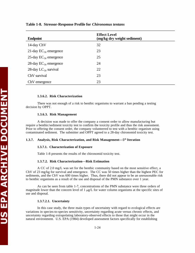
1-24
Table 1-8. Stressor-Response Profile for Chironomus tentans
EndpointEffect Level(mg/kg dry weight sediment)
14-day ChV 32
21-day EC50 emergence 23
25-day EC50 emergence 25
28-day EC50 emergence 24
28-day LC50 survival 22
ChV survival 23
ChV emergence 23
1.3.6.2. Risk Characterization
There was not enough of a risk to benthic organisms to warrant a ban pending a testingdecision by OPPT.
1.3.6.3. Risk Management
A decision was made to offer the company a consent order to allow manufacturing butrequire a benthic/sediment toxicity test to confirm the toxicity profile and thus the risk assessment. Prior to offering the consent order, the company volunteered to test with a benthic organism usingcontaminated sediment. The submitter and OPPT agreed to a 28-day chironomid toxicity test.
1.3.7. Analysis, Risk Characterization, and Risk Management—5th Iteration
1.3.7.1. Characterization of Exposure
Table 1-8 presents the results of the chironomid toxicity test.
1.3.7.2. Risk Characterization—Risk Estimation
A CC of 2.0 mg/L was set for the benthic community based on the most sensitive effect, aChV of 23 mg/kg for survival and emergence. The CC was 50 times higher than the highest PEC forsediments, and the ChV was 600 times higher. Thus, there did not appear to be an unreasonable riskto benthic organisms as a result of the use and disposal of the PMN substance over 1 year.
As can be seen from table 1-7, concentrations of the PMN substance were three orders ofmagnitude lower than the concern level of 1 :g/L for water column organisms at the specific sites ofuse and disposal.
1.3.7.2.1. Uncertainty
In this case study, the three main types of uncertainty with regard to ecological effects arevariations in species-to-species sensitivity, uncertainty regarding acute versus chronic effects, anduncertainty regarding extrapolating laboratory-observed effects to those that might occur in thenatural environment. U.S. EPA (1984) developed assessment factors specifically for establishing

1-25
concentrations of concern for PMN substances. Use of these factors is not intended to establish a"safe" level for a particular substance, but rather to identify a concentration which, if equaled orexceeded, could result in some adverse ecological effects. Such a finding provides the rationale forrequesting either actual testing of the PMN substance or more specific information about fate andexposure. Naturally, there are other types of uncertainty, such as the effects of the PMN substanceon adult rather than juvenile fish. Such types of uncertainty are research issues.
In the case of the exposure profile, an important aspect of uncertainty has to do with theactual duration of exposure. The PDM3 model predicts only the number of days out of 1 year thatthe CC will be exceeded (table 1-4). These days are not necessarily consecutive days. Thus, onlyflow rates could be used to account for seasonal variation. The presence or absence of critical lifestages of aquatic organisms cannot be accounted for with this type of analysis. In addition, thegeneric nature of the assessment precludes identification of specific biota.
1.3.7.2.2. Risk Description—Ecological Risk Summary
This case study demonstrates the validity of QSAR in establishing toxicity profiles for waterquality organisms (fish, invertebrates, and algae). In this case, the chemical structure indicated thatthe PMN substance was closely analogous to chemicals known to behave like neutral organiccompounds. The high Kow indicated that the compound would not be acutely toxic, and this wasconfirmed by an actual test with a surrogate fish species. Actual chronic toxicity testing confirmedthe QSAR-predicted chronic toxicity (within an order of magnitude). EPA's experience with otherhigh-Kow compounds such as hexachlorobenzene and chloroparaffins further confirms the chronicallytoxic nature of such compounds. The predictions for chironomid toxicity did not agree with the actualtest data. QSARs have not been developed for benthic organisms simply because not enough testdata are available to permit such analyses.
The use of QSAR is not limited to neutral organic compounds. Currently, there are QSARsavailable for compounds that show more specific modes of toxicity or excess toxicity over the neutralorganics. Examples include acrylates, methacrylates, aldehydes, anilines, benzotriazoles, esters,phenols, and epoxides (Auer et al., 1990; Clements, 1988).
Because the CCs were exceeded enough times out of 1 year, the PDM3 model indicated arisk to aquatic organisms. When actual sites were analyzed using EXAMS II, no unreasonable riskswere identified.
1.3.7.2.3. Ecological Significance
There appears to be no unreasonable risks to pelagic and benthic organisms at the identifieduse sites. The potential risk posed by the PMN substance bioaccumulating through the aquatic foodweb was thought not to be significant.
1.3.7.2.4. Spatial and Temporal Patterns of the Effects
CBI restrictions preclude revealing the uses and specific sites for the PMN substance. However, the technical assessors identified important river systems that could be affected by thisPMN substance. Thus, if there was a risk, the effects are not likely to be localized.
1.3.7.2.5. Recovery Potential
The PMN substance is a neutral hydrophobic chemical. This mode of toxicity is akin to asimple narcosis type of action (Auer et al., 1990; Veith and Broderius, 1990) that is reversible ifexposure to the toxicant is terminated before lethality or death occurs.

1-26
The recovery potential was not evaluated. Short-term pulsed exposure is not likely to causeadverse effects. However, continued exposure is likely to cause some impact to benthic organisms,but not enough of an impact to regulate.
1.3.8. Risk Management—Final Decision
The risk managers agreed that the PMN substance posed no unreasonable risks to pelagicaquatic organisms at the specific sites of use and disposal. However, there could be risks at othersites through the use and disposal of the PMN substance. Therefore, the final disposition was aSNUR including a restriction against releasing concentrations higher than 1 :g/L (the concern levelfor the PMN substance). The manufacturer must submit a significant new use notice if it wants touse the PMN substance at sites other than the ones identified in its submission.
Comments on Characterization of Exposure
Strengths of the case study include:
! The case study used a well-known model for estimating exposure in aquaticenvironments. The case study illustrates how such models can be employed.
! The study relied on a pilot treatment study to estimate removal of the chemical ina POTW (i.e., with the sludge).
! The study provides a good example of the PMN review process.
Limitations include:
! The choice of Kow or Koc value is a critical aspect of the study that should bediscussed. Also, the case study should include a discussion of the sensitivity ofthe results to selection of Kow values.
! Chemical properties indicated a tendency to bind suspended particles, yet therewas no exposure pathway involving chemical 6 sediment 6 suspended particle 6feeding or bioconcentration.

1-27
Comments on Characterization of Exposure (continued)
! The exposure analysis should have considered the fate of the sludge from thePOTW. Such sludge is often applied to agricultural or forest land.
! More detail about the discharges should be given, even if it is something like"one large" or "several small."
! For chemical products that are mixtures, there may be a large number ofchemicals present, and this may contribute to variability in estimates as well asmeasurements. The mixture can result in exposure conditions in theenvironment different from those for the original material.
Author's comments:
! The simple stream flow model offers a conservative estimate of exposure byassuming instantaneous mixing and dispersion of the chemical. The model doesnot take into account any losses due to factors such as volatilization,partitioning, or chemical or biological degradation after release. Because ofthe paucity of data and information about exposure, the use of conservativemodels is justified.
! The PDM3 model is an improvement over the simple stream flow models in thatthe temporal nature of exposure can be evaluated. Thus, a risk manager can beadvised as to how often a particular concentration is likely to be exceeded.
! The above two models estimate chemical concentrations in the water columnonly. As demonstrated in the study, more in-depth models such as EXAMS IIcan be used to estimate chemical concentrations both in the water column andsediments when sufficient data are available.
Comments on Characterization of Ecological Effects
Strengths of the case study include:
! The case study illustrates the iterative approach associated with the evaluationof a PMN chemical.
Limitations include:
! Estimating a concern level for sediment organisms based on earthworm data isnot appropriate because earthworms exchange gases with air and sedimentorganisms exchange gases with water. The statement that sediment organiccarbon will mitigate toxicity 10 times more than soil or peat carbon requiresadditional support.

1-28
Comments on Characterization of Ecological Effects (continued)
! The authors should give a good rationale for their approach to estimatingsediment toxicity and tell why it is better than the equilibrium partitioningmethod other offices in EPA are using, or they should use the equilibriumpartitioning method.
! The case study should not state that it demonstrates the validity of QSAR inestablishing toxicity profiles. The estimated 21-day chronic value of 0.100 was230-fold lower than the test results (tables 1-6 and 1-8). A single case studywould not be sufficient to demonstrate the validity of using QSAR to establishtoxicity profiles, no matter what might have been shown.
Author's comments:
! The use of SAR is commonplace within OPPT because TSCA does not requirethe completion of test data prior to the submission of a PMN. The track recordwith SAR is extremely good (Nabholz et al., 1993b) and has resulted indropping low- risk chemicals from review and regulating high-risk chemicalswithout measured data on the chemical. Provided sound expert judgment isemployed, SAR can identify whether acute or chronic tests (or both) are needed.
! The use of surrogate species at different trophic levels (e.g., fish, daphnids,algae, benthic organisms) permits one to evaluate which organisms are mostsensitive to a given xenobiotic. While many argue that the commonly usedsurrogates may not be as sensitive as those in the wild, both industry andgovernment agree that it is the most practical way to evaluate the ecologicaleffects of chemicals. Because many industrial chemicals are used in a widearray of industries as well as consumer products, identifying specific biota (atthe species level) is often impossible.
! The cost of larger scale studies such as laboratory microcosms and fieldmesocosms has precluded their use to assess the ecological effects of newchemicals. However, OPPT is initiating field mesocosm studies at the ERL-Duluth to evaluate how well laboratory tests predict effects in the field.

1-29
Comments on Characterization of Ecological Effects (continued)
! Comparing a fish 14-day LC50 with an earthworm 14-day LC50 value in anartificial soil was the only available way at the time to estimate the effect thatorganic matter would have on the bioavailability of an organic chemical insediments. It was known that (1) earthworms interacted intimately with soil porewater, (2) the toxicity of organic chemicals in soil toward earthworms could bepredicted by relating molar concentration in soil pore water to the chemical'sKow (van Gestel and Ma, 1990), (3) Kow was highly correlated with Koc, and (4)the amount of organic matter in sediments strongly influenced the amount oforganic chemical that could be absorbed by sediments. It was a simple andvalid extrapolation to use earthworms as a surrogate for benthic organisms. Inaddition, when the OPPT assessment team conferred with the submitter'sassessors, the submitter accepted OPPT's best estimate given the level ofknowledge and available data that existed at the time.
! Sediment organic matter was expected to be more efficient than the ground peatused in the artificial soil of the earthworm toxicity test because sediment organicmatter is generally more finely divided due to more processing by invertebratesand partial degradation by microbes. Sediment organic matter was expected tohave a much greater surface area to volume ratio than the peat and, therefore,a much greater absorptive area to reduce the bioavailability of organicchemicals with high Kow values (i.e., >4.2).
Comments on Risk Characterization
Strengths of the case study include:
! The risk characterization appeared to be adequate for a management decision.
! The case study illustrates the PMN risk assessment process.
Limitations include:
! The summary table of the major assumptions and estimates used at variousstages of the process (table 1-4) should have included some information on themagnitude of uncertainty associated with each of these estimates orassumptions.
! The risk assessment methods employed do not distinguish risks to individualsfrom risks to populations. In some cases "individuals" are the organizationallevel of interest, while in other cases it is the "population."

1-30
Comments on Risk Characterization (continued)
! It was pointed out that assessment factors were developed in 1984 andcontinued to evolve along with the PMN process. The case study should includethe method used to derive the assessment factors and a brief statement of thehistory of these factors.
! The case study should clarify the difference between "uncertainty" in thestatistical sense and "uncertainty" as it is addressed by using "assessmentfactors."
! Assigning an assessment factor of "1" to field toxicity data is not appropriatebecause field data are site-specific, and the data may not be directlytransferable to other sites where the chemical might be used or released.
! The available information suggested that risks to benthic organisms wereprobably more important than those to pelagic organisms. Yet, the process wascarried out in a specific manner that emphasized the studies on pelagicorganisms first. It was pointed out that this was policy.
! If disposal options were considered along with the risk assessment, then variousoptions could have been considered early in the process. Such mitigation couldbe included as an iteration.
! If "acceptable" concentrations were first identified, then it would be possible toestimate acceptable loadings.
General reviewer comments:
! The case study description of interactions between risk assessors and riskmanagers led the reviewers to discuss the following:
-- Who is the risk manager? It appears to be a manager at EPA, but themanager at the company also can manage risk by deciding not to testfurther and abandoning the chemical, or he could deal with potentialexposure by treating the waste stream or making process changes.
-- It might be useful to develop a framework for risk managers similar tothat for risk assessors. Both frameworks should contain sections oninteraction with the other and on mitigation.
! The example chemical does not indicate how well the process works for othertypes of chemicals. Narcoleptic chemicals are the easiest chemicals to model fortoxicity. Reactive toxicants often cannot be modeled simply, if at all, and theyare usually more toxic or hazardous.

1-31
Comments on Risk Characterization (continued)
! Reviewers discussed the use of "probabilistic" risk assessment. It was notedthat this is the direction in which EPA is going. A question was raisedregarding whether these quantitative methods would be understandable to therisk manager. Some experience indicates that they would.
Author's comments:
! The Quotient Method is the most common ecological risk assessment methodused in OPPT for new and existing chemicals. It also is used by the Office ofPesticide Programs. The Quotient Method is easy to use, is mutually acceptedby industry and EPA, and is amenable to the ecological effects and exposuredata available to OPPT under TSCA.
! One disadvantage of this method is the uncertainty about the degree of riskwhen quotients approach, but do not equal, 1. Also, it is difficult to quantifyrisks to assessment endpoints when most ecological risk assessments underTSCA are generic. While the risks to measurement endpoints can be quantified,extrapolating such risks to the population or community level is impossibleunless simulation models are employed. OPPT is evaluating developmentalversions of population and ecosystem models for use with existing chemicals;however, due to the volume of PMNs, their use is not practical at this time. Thisis particularly true for ecosystem models that require mainframe or high-speed/high-memory computers. Thus, only qualitative inferences can be madebetween measurement and assessment endpoints.
! Since 1979, OPPT has assessed the environmental toxicity of over 24,000chemicals submitted under Section 5 of TSCA. Although only 4.8 percent ofthose chemicals had any environmental toxicity information submitted with them,OPPT has been able to use chemical structure and commonly measuredphysical/chemical properties to model the aquatic toxicity of many classes ofreactive toxicants, including 64 classes of organic chemicals that have sometype of specific toxicity in addition to narcosis.

1-32
1.4. REFERENCES
Auer, C.M.; Nabholz, J.V.; Baetcke, K.P. (1990) Mode of action and the assessment of chemicalhazards in the presence of limited data: use of structure-activity relationships (SAR) underTSCA, Section 5. Environ. Health Perspect. 87:183-197.
Banerjee, S.; Yalkowsky, S.H.; Valvani, S.C. (1980) Water solubility and octanol/water partitioncoefficients of organics. Limitations of the solubility-partition coefficient correlation. Environ. Science Technol. 14:1227-1229.
Barnthouse, L.W.; Suter, G.W.; Bartell, S.M.; Beauchamp, J.J.; Gardner, R.H.; Linder, E.; O'Neill,R.V.; Rosen, A.E. (1986) User's manual for ecological risk assessment. Oak RidgeNational Laboratory. ORNL Publ. No. 2679.
Broderius, S.J.; Russom, C.L. (1989) Mode of action-specific QSAR models for predicting acute andchronic toxicity of industrial chemicals to aquatic organisms. U.S. Environmental ProtectionAgency. Duluth, MN: Environmental Research Laboratory. Deliverable No. 81421.
Burns, L.A. (1989) Exposure analysis modeling system: user's guide for EXAMS II version 2.94.Athens, GA: U.S. Environmental Protection Agency.
Clements, R. (1983) Environmental effects of regulatory concern under TSCA—a positionpaper. Environmental Effects Branch, Health and Environmental Review Division (7403),Office of Toxic Substances, U.S. Environmental Protection Agency, Washington, DC.
Clements, R. (1988) Estimating toxicity of industrial chemicals to aquatic organisms usingstructure-activity relationships. U.S. Environmental Protection Agency, Washington, DC.EPA 560-6-88-001. Available from: NTIS, Springfield, VA, PB89-117592.
Grain, C.F. (1982) Vapor pressure. In: Lyman, W.J.; Reehl, W.; Rosenblatt, D.H., eds. Handbook ofchemical property estimation methods, environmental behavior of organic compounds.New York, NY: McGraw-Hill Co.
Hermens, J.; Canton, H.; Janssen, P.; DeJong, R. (1984) Quantitative structure-activity relationshipsand toxicity studies of mixtures of chemicals with anesthetic potency: acute lethal andsublethal toxicity to Daphnia magna. Aquat. Toxicol. 5:143-154. (also in Clements, 1988).
Karickhoff, S.W.; Brown, D.S.; Scott, T.A. (1979) Sorption of hydrophobic pollutants on naturalsediments. Water Res. 13:241-248.
Konemann, H. (1981) Quantitative structure-activity relationships in fish toxicity studies. Part 1:relationship for 50 industrial pollutants. Toxicology 19:209-221.
Leo, A.; Weininger, D. (1985) CLOGP version 3.3. estimation of the n-octanol/water partitioncoefficient for organics in the TSCA industrial inventory. Claremont, CA: PomonaCollege.
Lipnick, R.L. (1985) Validation and extension of fish toxicity QSARs and interspecies comparisonsfor certain classes of organic chemicals. In: Tichy, M., ed. Toxicology andxenobiochemistry. 8:39-52.
Nabholz, J.V. (1991) Environmental hazard and risk assessment under the United States ToxicSubstances Control Act. The science of the total environment. 109/110:649-665.

1-33
Nabholz, J.V. (in preparation) Estimating toxicity of industrial chemicals to aquatic organisms usingstructure-activity relationships.
Nabholz, J.V.; Miller, P.; Zeeman, M. (1993a) Environmental and risk assessment of new chemicalsunder the Toxic Substances Control Act (TSCA) Section Five. In: Landis, W.G.; Hughes,J.S.; Lewis, M.A., eds. Environmental toxicology and risk assessment. American Societyfor Testing and Materials, Philadelphia, PA. ASTM STP 1179.
Nabholz, J.V.; Clements, R.G.; Zeeman, M.G.; Osborn, K.C.; Wedge, R. (1993b) Validation ofstructure-activity relationships used by EPA's Office of Pollution Prevention and Toxics forthe environmental hazard assessment of industrial chemicals. In: Gorsuch, J.W.; Dwyer, F.J.;Ingersoll, C.G.; LaPoint, T.W., eds. Environmental toxicology and risk assessment.American Society for Testing and Materials, Philadelphia, PA. ASTM STP 1216.
Rodier, D.J.; Mauriello, D. (1993) The quotient method of ecological risk assessment and modelingunder TSCA: a review. In: Landis, W.G.; Hughes, J.S.; Lewis, M.A, eds. Environmentaltoxicology and risk assessment. American Society for Testing and Materials, Philadelphia,PA. ASTM STP 1179.
Smrchek, J.; Clements, R.; Morcock, R.; Roberts, R. (1993) Assessing ecological hazard underTSCA: methods and evaluation of data. In: Landis, W.G.; Hughes, J.S.; Lewis, M.A., eds.Environmental toxicology and risk assessment. American Society for Testing andMaterials, Philadelphia, PA. ASTM STP 1179.
Suter, G.W. (1990) Endpoints for regional ecological risk assessment. Environ. Manage. 14:9-23.
TSCA. (1976) Toxic Substances Control Act, PL 94-46, October 11, 1976, Stat. 90:2003.
U.S. Environmental Protection Agency. (1982) Surrogate species workshop. Environmental EffectsBranch, Health and Environmental Review Division (7403), Office of Toxic Substances, U.S.Environmental Protection Agency, Washington, DC.
U.S. Environmental Protection Agency. (1983) Testing for environmental effects under the ToxicSubstances Control Act. Environmental Effects Branch, Health and Environmental ReviewDivision (7403), Office of Toxic Substances, U.S. Environmental Protection Agency,Washington, DC.
U.S. Environmental Protection Agency. (1984) Estimating concern levels for concentrations ofchemical substances in the environment. Environmental Effects Branch, Health andEnvironmental Review Division (7403), Office of Toxic Substances, U.S. EnvironmentalProtection Agency, Washington, DC.
U.S. Environmental Protection Agency. (1985) Toxic Substances Control Act test guidelines, finalrules. Federal Register 50(188):39252-39516.
U.S. Environmental Protection Agency. (1986) New chemical review process manual. Office ofToxic Substances, U.S. Environmental Protection Agency, Washington, DC. EPA 560/3-86-002.
U.S. Environmental Protection Agency. (1988) User's guide to PDM3, final report. EPA ContractNo. 68-02-4254, Task No. 117. Exposure Assessment Branch, Exposure Evaluation Division(7403), Office of Toxic Substances, U.S. Environmental Protection Agency, Washington,DC.

1-34
U.S. Environmental Protection Agency. (1992) Framework for ecological risk assessment. RiskAssessment Forum, Washington, DC. EPA 630/R-92/001.
U.S. Environmental Protection Agency. (1993) PMN Ecotox Database: a data base ofenvironmental toxicity studies which are protected by confidential business information(CBI). Environmental Effects Branch, Health and Environmental Review Division (7403),Office of Toxic Substances, U.S. Environmental Protection Agency, Washington, DC.
van Gestel, C.A.M.; Ma, W.-C. (1990) An approach to quantitative structure-activity relationships(QSARs) in earthworm toxicity tests. Chemosphere 20:1023-1033.
Veith, G.D.; Call, D.J.; Brooke, L.T. (1983) Structure-activity relationships for the fathead minnow,Pimephales promelas: narcotic industrial chemicals. Can. J. Fish. Aquat. Sci. 40:743-748.(also in Clements, 1988).
Veith, G.D.; Broderius, S.J. (1990) Rules for distinguishing toxicants that cause type I and type IInarcosis syndromes. Environ. Health Perspect. 87:207-211.
Zeeman, M.; Nabholz, J.V.; Clements, R.G. (1993) The development of SAR/QSAR for the useunder EPA's Toxic Substances Control Act (TSCA): an introduction. In: Gorsuch, F.J.;Dwyer, F.J.; Ingersoll, C.G.; LaPoint, T.W., eds. Environmental toxicology and riskassessment: 2nd volume. American Society for Testing and Materials, Philadelphia, PA.ASTM STP 1216.

APPENDIX A
QSARS BETWEEN NEUTRAL ORGANIC CHEMICALS AND FISH AND GREEN ALGAL TOXICITY
1-A1

QSARS BETWEEN NEUTRAL ORGANIC CHEMICALS AND FISH CHRONIC VALUES
(Broderius and Russom, 1989)
! Log NOEC (mol/L) = !0.878 Log Kow ! 2.40
n = 20 r2 = 0.911 s = 0.335
! Log LOEC (mol/L) = !0.862 Log Kow ! 2.16
n = 20 r2 = 0.913 s = 0.325
! Log ChV (mol/L) = !0.870 Log Kow ! 2.28
n = 20 r2 = 0.914 s = 0.327
! Log ChV (mg/L) = antilog ChV (mol/L) * mw
QSARS BETWEEN NEUTRAL ORGANIC CHEMICALS AND GREEN ALGAE TOXICITY (GROWTH) (Nabholz, in preparation)
! Log ChV (mmol/L) = 0.036 ! 0.634 Log Kow
n = 6 r2 = 0.99
! Log 96-h EC50 (mmol/L) = 1.48 ! 0.869 Log Kow
n = 22 r2 = 0.93
Please note: The QSARs referenced here and elsewhere in the report are now available as a computer program called ECOSAR (EPA-748-F-93-002). Limited copies are available from the National Center for Environmental Publications and Information, U.S. EPA, 26 West Martin Luther King Drive, Cincinnati, OH 45268 (513-569-7985). In addition, copies may be obtained from:
! U.S. Government Printing Office, Superintendent of Documents, ATTN: Electronic Product Sales Coordinator, P.O. Box 37082, Washington, DC 20013-7082 (202-512-1530);
! Federal Bulletin Board, U.S. Government Printing Office of Electronic Information Dissemination Services (202-512-1524); or
! National Technical Information Service, U.S. Department of Commerce, 5285 Port Royal Road, Springfield, VA 22161 (703-487-4650) (order as computer program PB94-500485).
1-A2

APPENDIX B
INPUT AND OUTPUT PARAMETERSFOR EXAMS II
1-B1

INPUT PARAMETERS FOR EXAMS II
EXAMS II estimates exposure, fate, and persistence of an organic chemical after being released into an aquatic ecosystem (Burns, 1989). EXAMS II requires input of data into three files that describe the chemical, the environment, and the chemical loading to the environment.
Critical inputs to the chemistry file for this example were the water solubility, octanol-water partition coefficient (Kow), soil/sediment organic carbon-water partition coefficient (Koc), and biodegradation rate constant. These parameters are important in modeling the test chemical partitions between the water column and sediments. This particular analysis used a log Kow of 6.56.
The environment file was culled from a set of predefined or canonical environments. Data including stream geometry and surface water flow rates are included here. Two important parameters that were user-defined in this example were the benthic and suspended sediment organic carbon content and the concentration of microorganisms in the sediments active in the biodegradation of the compound. The mass of test chemical released per unit time is entered into the loading file.
OUTPUT OF EXAMS II
The EXAMS II output includes tables summarizing test chemical properties; environmental characteristics; chemical loadings; steady-state mean, minimum, and maximum concentrations in various environmental compartments; and an exposure analysis summary (see example below).
EXAMPLE OUTPUT OF EXAMS (NOT CASE STUDY PMN)
Exposure (maximum steady-state concentrations):
Water column: 7.884E-03 mg/L dissolved; total = 8.255E-03 mg/L
Benthic sediments:
Biota (:g/g dry weight):
Fate:
Total steady-state accumulation:
Total chemical load:
Persistence:
7.377E-03 mg/L dissolved in pore water; maximum total concentration = 33.1 mg/kg (dry weight)
Plankton: 7.68E+03 Benthos: 7.18E+03
494 kg, with 0.29 percent in the water column and 99.71 percent in the benthic sediments.
27 kg/month. Disposition: 0.00 percent chemically transformed, 0.00 percent biotransformed, 0.00 percent volatilized, and 100.00 percent exported via other pathways.
After 16.0 months of recovery time, the water column had lost 65.82 percent of its initial chemical burden; the benthic zone had lost 60.08 percent; systemwide total loss of chemical = 60.1 percent. Five half-lives (>95 percent cleanup) thus require about 60 months.
1-B2

SECTION TWO
ECOLOGICAL RISK ASSESSMENT CASE STUDY:
RISK ASSESSMENT FOR THE RELEASE OF RECOMBINANT RHIZOBIA AT A SMALL-SCALE AGRICULTURAL FIELD SITE

AUTHORS AND REVIEWERS
AUTHORS
Gwendolyn McClungOffice of Pollution Prevention and ToxicsU.S. Environmental Protection AgencyWashington, DC
Philip G. SayreOffice of Pollution Prevention and ToxicsU.S. Environmental Protection AgencyWashington, DC
REVIEWERS
Joseph E. Lepo (Lead Reviewer)Center for Environmental Diagnostics
and BioremediationUniversity of West FloridaGulf Breeze, FL
Gregory R. BiddingerExxon Biomedical Sciences, Inc.East Millstone, NJ
Joel S. BrownUniversity of Illinois at ChicagoChicago, IL
Herbert GroverBenchmark Environmental CorporationAlbuquerque, NM
Thomas SibleyFisheries Research InstituteUniversity of WashingtonSeattle, WA
Frieda B. TaubSchool of Fisheries
University of Washington Seattle, WA
2-2
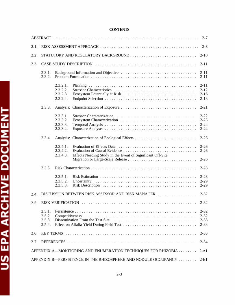
CONTENTS
ABSTRACT . . . . . . . . . . . . . . . . . . . . . . . . . . . . . . . . . . . . . . . . . . . . . . . . . . . . . . . . . . . . . . . 2-7
2.1. RISK ASSESSMENT APPROACH . . . . . . . . . . . . . . . . . . . . . . . . . . . . . . . . . . . . . . . . . . . 2-8
2.2. STATUTORY AND REGULATORY BACKGROUND . . . . . . . . . . . . . . . . . . . . . . . . . . . . . 2-10
2.3. CASE STUDY DESCRIPTION . . . . . . . . . . . . . . . . . . . . . . . . . . . . . . . . . . . . . . . . . . . . 2-11
2.3.1. Background Information and Objective . . . . . . . . . . . . . . . . . . . . . . . . . . . . . . . . . 2-112.3.2. Problem Formulation . . . . . . . . . . . . . . . . . . . . . . . . . . . . . . . . . . . . . . . . . . . . . . 2-11
2.3.2.1. Planning . . . . . . . . . . . . . . . . . . . . . . . . . . . . . . . . . . . . . . . . . . . . . . . 2-112.3.2.2. Stressor Characteristics . . . . . . . . . . . . . . . . . . . . . . . . . . . . . . . . . . . . 2-122.3.2.3. Ecosystem Potentially at Risk . . . . . . . . . . . . . . . . . . . . . . . . . . . . . . . . 2-162.3.2.4. Endpoint Selection . . . . . . . . . . . . . . . . . . . . . . . . . . . . . . . . . . . . . . . . 2-18
2.3.3. Analysis: Characterization of Exposure . . . . . . . . . . . . . . . . . . . . . . . . . . . . . . . . . 2-21
2.3.3.1. Stressor Characterization . . . . . . . . . . . . . . . . . . . . . . . . . . . . . . . . . . . 2-222.3.3.2. Ecosystem Characterization . . . . . . . . . . . . . . . . . . . . . . . . . . . . . . . . . 2-232.3.3.3. Temporal Analysis . . . . . . . . . . . . . . . . . . . . . . . . . . . . . . . . . . . . . . . . 2-242.3.3.4. Exposure Analyses . . . . . . . . . . . . . . . . . . . . . . . . . . . . . . . . . . . . . . . . 2-24
2.3.4. Analysis: Characterization of Ecological Effects . . . . . . . . . . . . . . . . . . . . . . . . . . . 2-26
2.3.4.1. Evaluation of Effects Data . . . . . . . . . . . . . . . . . . . . . . . . . . . . . . . . . . 2-262.3.4.2. Evaluation of Causal Evidence . . . . . . . . . . . . . . . . . . . . . . . . . . . . . . . . 2-262.3.4.3. Effects Needing Study in the Event of Significant Off-Site
Migration or Large-Scale Release . . . . . . . . . . . . . . . . . . . . . . . . . . . . . . 2-26
2.3.5. Risk Characterization . . . . . . . . . . . . . . . . . . . . . . . . . . . . . . . . . . . . . . . . . . . . . . 2-28
2.3.5.1. Risk Estimation . . . . . . . . . . . . . . . . . . . . . . . . . . . . . . . . . . . . . . . . . . 2-282.3.5.2. Uncertainty . . . . . . . . . . . . . . . . . . . . . . . . . . . . . . . . . . . . . . . . . . . . . 2-292.3.5.3. Risk Description . . . . . . . . . . . . . . . . . . . . . . . . . . . . . . . . . . . . . . . . . 2-29
2.4. DISCUSSION BETWEEN RISK ASSESSOR AND RISK MANAGER . . . . . . . . . . . . . . . . . 2-32
2.5. RISK VERIFICATION . . . . . . . . . . . . . . . . . . . . . . . . . . . . . . . . . . . . . . . . . . . . . . . . . . 2-32
2.5.1. Persistence . . . . . . . . . . . . . . . . . . . . . . . . . . . . . . . . . . . . . . . . . . . . . . . . . . . . . 2-322.5.2. Competitiveness . . . . . . . . . . . . . . . . . . . . . . . . . . . . . . . . . . . . . . . . . . . . . . . . . 2-322.5.3. Dissemination From the Test Site . . . . . . . . . . . . . . . . . . . . . . . . . . . . . . . . . . . . . 2-332.5.4. Effect on Alfalfa Yield During Field Test . . . . . . . . . . . . . . . . . . . . . . . . . . . . . . . . 2-33
2.6. KEY TERMS . . . . . . . . . . . . . . . . . . . . . . . . . . . . . . . . . . . . . . . . . . . . . . . . . . . . . . . . . 2-33
2.7. REFERENCES . . . . . . . . . . . . . . . . . . . . . . . . . . . . . . . . . . . . . . . . . . . . . . . . . . . . . . . . 2-34
APPENDIX A—MONITORING AND ENUMERATION TECHNIQUES FOR RHIZOBIA . . . . . . . . 2-A1
APPENDIX B—PERSISTENCE IN THE RHIZOSPHERE AND NODULE OCCUPANCY . . . . . . . . 2-B1
2-3

CONTENTS (continued)
APPENDIX C—RHIZOBIAL DISPERSION AND MIGRATION . . . . . . . . . . . . . . . . . . . . . . . . . 2-C1
APPENDIX D—STRAIN COMPARISON AND COMPETITION TESTS . . . . . . . . . . . . . . . . . . . 2-D1
APPENDIX E—RHIZOBIAL CULTURE VIABILITY . . . . . . . . . . . . . . . . . . . . . . . . . . . . . . . . . 2-E1
APPENDIX F—ALFALFA YIELDS IN THE FIELD TESTS . . . . . . . . . . . . . . . . . . . . . . . . . . . . 2-F1
2-4
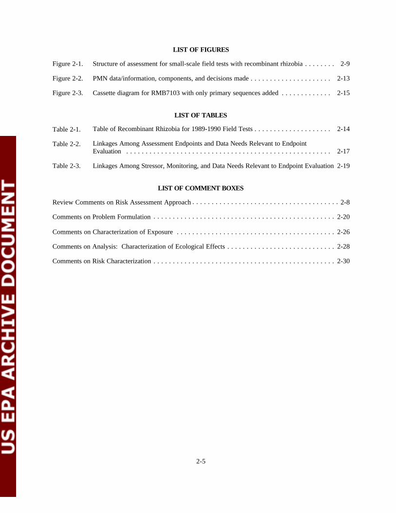
LIST OF FIGURES
Figure 2-1. Structure of assessment for small-scale field tests with recombinant rhizobia . . . . . . . . 2-9
Figure 2-2. PMN data/information, components, and decisions made . . . . . . . . . . . . . . . . . . . . . 2-13
Figure 2-3. Cassette diagram for RMB7103 with only primary sequences added . . . . . . . . . . . . . 2-15
LIST OF TABLES
Table 2-1. Table of Recombinant Rhizobia for 1989-1990 Field Tests . . . . . . . . . . . . . . . . . . . . 2-14
Table 2-2. Linkages Among Assessment Endpoints and Data Needs Relevant to EndpointEvaluation . . . . . . . . . . . . . . . . . . . . . . . . . . . . . . . . . . . . . . . . . . . . . . . . . . . . . 2-17
Table 2-3. Linkages Among Stressor, Monitoring, and Data Needs Relevant to Endpoint Evaluation 2-19
LIST OF COMMENT BOXES
Review Comments on Risk Assessment Approach . . . . . . . . . . . . . . . . . . . . . . . . . . . . . . . . . . . . . . 2-8
Comments on Problem Formulation . . . . . . . . . . . . . . . . . . . . . . . . . . . . . . . . . . . . . . . . . . . . . . . 2-20
Comments on Characterization of Exposure . . . . . . . . . . . . . . . . . . . . . . . . . . . . . . . . . . . . . . . . . 2-26
Comments on Analysis: Characterization of Ecological Effects . . . . . . . . . . . . . . . . . . . . . . . . . . . . 2-28
Comments on Risk Characterization . . . . . . . . . . . . . . . . . . . . . . . . . . . . . . . . . . . . . . . . . . . . . . . 2-30
2-5

LIST OF ACRONYMS
DNA deoxyribonucleic acid
EPA U.S. Environmental Protection Agency
FA fluorescent antibody
GEM genetically engineered microorganism
MDL minimum detection limit
MPN most probable number
OPPT Office of Pollution Prevention and Toxics
OTS Office of Toxic Substances
PMN premanufacture notice
RDM rhizobia-defined medium
TSCA Toxic Substances Control Act
2-6

ABSTRACT
This ecological risk assessment concerns a small-scale field test of genetically engineered Rhizobium meliloti strains. The strains were submitted in 1988 as part of a premanufacture notice (PMN) to the Office of Toxic Substances (OTS, currently the Office of Pollution Prevention and Toxics, OPPT) for tests to be conducted in 1989-1990. The rhizobia were genetically modified by the insertion of antibiotic resistance markers or by the addition of both antibiotic resistance and nif genes to enhance nitrogen fixation. R. meliloti form nodules and fix nitrogen in alfalfa (Medicago sativa), sweet clover (Melilotus), and fenugreek (Trigonella). The surrounding agroecosystem near Sun Prairie, Wisconsin, constituted the area of concern for ecological effects. Literature accounts of rhizobial movement, field test site characteristics, and field test design indicated that the microorganisms had only a minimal potential for migrating beyond the field test plot. The primary assessment endpoint examined during the small-scale field test was the potential for these recombinants to alter top growth of alfalfa. The ecological concerns for large-scale releases of recombinant rhizobia—such as increased growth of nontarget legumes, decreased growth of target legumes, spread of antibiotic resistance genes, nitrogen cycling disruption, and alteration of host range—were of low concern for the agroecosystem around the test site.
Actual data obtained from the small-scale field study confirmed the predictions in the OTS PMN risk assessment conducted in 1988 and those in this ecological risk assessment. Little horizontal, vertical, or aerial migration of R. meliloti occurred. The rhizobia primarily moved with the alfalfa root system. When compared with unmodified strains, recombinant rhizobia did not cause significant changes in nitrogen fixation, as measured indirectly by alfalfa yield. Recombinant strains did not out-compete parental strains, alleviating the concern for displacement of the indigenous rhizobia.
2-7

2.1. RISK ASSESSMENT APPROACH
This case study represents a typical risk assessment for a premanufacture notice (PMN) received by the U.S. Environmental Protection Agency's (EPA's) Office of Pollution Prevention and Toxics (OPPT). OPPT effectively evaluates the potential risk using the paradigm of "Risk = Hazard × Exposure" (Sayre, 1990). This paradigm is consistent with the Framework for Ecological Risk Assessment (U.S. EPA, 1992). Figure 2-1 demonstrates how the assessment was structured, using the framework report as guidance.
Since the framework report focuses on physical and chemical rather than biological stressors, the report does not adequately address certain aspects of this risk assessment. These include:
# the need for fate monitoring to build a data base of rhizobial behavior for larger-scale releases;
# the potential that in some cases the introduced deoxyribonucleic acid (DNA) might move from the genetically engineered microorganism (GEM) to other environmental recipients;
# consideration of field site design that limited microbial dissemination beyond the site, thereby alleviating the need for certain effects testing;
# the evaluation of exposure resulting from culturing and transporting GEMs to the field site; and
# construct considerations.
Reviewer Comments on Risk Assessment Approach
! As currently formulated, EPA's Framework for Ecological Risk Assessment does not address fundamental differences between biological stressors and chemical and physical stressors. These differences include concerns unique to living entities, such as replication, colonization, and genetic evolution. This case study should provide a useful model for assessing risks of future limited releases of genetically engineered microorganisms in agroecosystems.
! This case study does not address more general ecological risks, nor does it consider risks of large-scale or commercial release of GEMs. However, the study does serve as an important ground-breaking document because risk assessments of GEMs released into agroecosystems will become more common in the near future.
2-8

2-9

Reviewer Comments on Risk Assessment Approach (continued)
! The reviewers did not consider the application of the framework to microbial stressors an insurmountable barrier. However, they agreed that both the framework report and similar future case studies should acknowledge the unique properties and complexities of a living, changing stressor. The reviewers suggested that applying the framework to biotechnological risks—such as the release of GEMs—might require providing the framework audience with the biotechnological details needed for appraising the relative importance of the risk factors.
2.2. STATUTORY AND REGULATORY BACKGROUND
The "Coordinated Framework for Regulation of Biotechnology" (Office of Science and Technology Policy, 1986) explains that the Toxic Substances Control Act (TSCA) gives EPA the authority to review certain classes of biotechnology products. Under the coordinated framework, biotechnology products are regulated in accordance with the use of each product (Milewski, 1990). Uses of microorganisms not covered by other existing authorities (U.S. Department of Agriculture, Food and Drug Administration, EPA's Office of Pesticide Programs) are reviewed by EPA's OPPT under TSCA; thus, TSCA serves as a "gap-filling" statute. TSCA's applicability follows from the interpretation that microbes are chemical substances under TSCA. Candidates for review are limited to those commercial microorganisms that have been altered to contain genetic information from dissimilar source organisms. EPA describes as dissimilar those organisms produced using DNA from different taxonomic genera. Such microorganisms are considered "intergeneric." EPA does not regulate the use of naturally occurring rhizobial inoculants.
TSCA applies only to products developed for commercial purposes, whether for contained systems or environmental releases. Under Section 5 of TSCA, manufacturers and importers of intergeneric microorganisms must submit a PMN at least 90 days prior to beginning manufacture or import. Under TSCA authority, OPPT can require information on microbial biotechnology products in order to identify potential hazards and exposures. OPPT also can require testing a microbial biotechnology product that may present an unreasonable risk of injury to human health or the environment or that is produced in substantial quantities and may result in substantial environmental release or substantial human exposure. Finally, OPPT can restrict the production, processing, distribution, use, and disposal of a microbial biotechnology product if it presents an unreasonable risk of injury to human health or the environment.
Because TSCA applies only to microorganisms developed for commercial purposes, EPA currently requests that industry voluntarily comply with the PMN reporting requirements for any commercial research and development field test that involves the release of intergeneric microorganisms involving a TSCA use. As a result, the PMN submission for the small-scale field test of genetically engineered strains of Rhizobium meliloti, the subject of this ecological risk assessment, was submitted on a voluntary basis by Biotechnica Agriculture, Inc., in 1988. Approval of the field test resulted in the issuance of a 5(e) Consent Order, which bound the company to the protocols, monitoring procedures, and data collection approved by EPA.
2.3. CASE STUDY DESCRIPTION
2.3.1. Background Information and Objective
This case study focuses primarily on the small-scale field testing of four recombinant strains of R. meliloti. Rhizobia, a general term for various species of the genus Rhizobium, are Gram-negative,
2-10

motile, rod-shaped, aerobic bacteria that infect legume roots. A symbiotic relationship forms in which the bacteria fix atmospheric nitrogen, providing ammonium for protein production in the plant. In exchange, the bacteria obtain energy from the plant in the form of photosynthate, specifically dicarboxylates.
The various species and biovars of Rhizobium have been designated according to the types of legume plants they infect, such as alfalfa, clovers, beans, vetch, or lotus. The specificity of infection by certain species or biovars of Rhizobium has led to the loose designation of "cross-inoculation" groups (Alexander, 1977). For example, the alfalfa group consists of R. meliloti, which is capable of infecting not only alfalfa (Medicago), but sweet clover (Melilotus) and fenugreek (Trigonella).
The symbiotic relationship between rhizobia and legumes is of great importance in agriculture, as legumes typically are not fertilized with nitrogen if rhizobia are present. In fact, high nitrogen contents in soils actually suppress nitrogen fixation by the nodules. More important, symbiotic nitrogen fixation contributes greatly to the nitrogen cycle. In association with alfalfa, rhizobia fix nitrogen vigorously, perhaps fixing between 125 and 335 kg of nitrogen per hectare each year (Alexander, 1977).
This case study has two purposes. First, the case study will examine the information submitted and used during the OPPT risk assessment to determine whether the framework assessment process can use the information as efficiently. Second, the case study will examine the data generated from the field to determine how accurately the risk assessment process predicted risks associated with the field test.
The area of concern for possible adverse ecological impacts is the surrounding agroecosystem. Ecological concerns are contingent on the ability of the rhizobia to survive and spread beyond the immediate area of the field site.
2.3.2. Problem Formulation
2.3.2.1. Planning
This risk assessment focused on determining the potential adverse effects of conducting a small-scale field test with recombinant rhizobia. However, the data gathered from the field site also may prove useful in projecting adverse effects that could result from a large- or commercial-scale release. Before such a release occurs, the potential ecological effects for a large-scale release need to be addressed.
The PMN submission supplied laboratory data on the microorganism identity, construct information, and microorganism characteristics and behavior. Greenhouse data addressed the effects on alfalfa (yield data), survival, and competitiveness of the recombinant strains (nodule occupancy). These data contributed to the decision-making process for approval of the small-scale field test. Field test protocols and a site evaluation conducted prior to the field tests also helped reach the decision to approve the small-scale field test of these recombinant rhizobia.
Figure 2-2 illustrates the various components of the risk assessment process for PMNs, from the data submissions through the decision-making processes prior to approval for commercial release. The field test design included several approaches to evaluating adverse effects from small-scale releases of recombinant rhizobia. Yields of alfalfa were an indirect measure of changes in the nitrogen-fixing ability of rhizobial strains. Nodule occupancy indicated competitiveness of the rhizobial strains with the indigenous rhizobial populations. The test design also included plans to measure the persistence of the microorganism in the rhizosphere. Finally, to test the prediction that only limited dissemination of the recombinant microorganisms beyond the site would occur, the test design included monitoring both soil and air for the presence of these microorganisms.
2-11

2.3.2.2. Stressor Characteristics
The primary stressors in this case study are the recombinant rhizobia, as opposed to chemical or physical stressors. In this study, the stressor has the potential to split into subcomponents of a biological nature (pathogenicity, altered legume growth resulting from the microbe) and subcomponents of a chemical nature (production of toxins, detrimental metabolites, and overproduction of nitrate).
As with chemical stressors, characterizing the recombinant microbes to predict their potential adverse effects constitutes a critical component for the risk assessment. For the recombinant microorganism, characterization includes a description of the donor and recipient microorganisms, including their taxonomic derivation. The phenotypic traits of most GEMs reviewed in OPPT are encoded and analyzed with a PC-microcomputer version of the "Micro-IS" software package; this data system was originally developed by the National Institutes of Health (Segal, 1988). A description of the techniques used to construct the PMN microorganism also contributes to characterization of the GEM.
The final step for GEM identification involves verifying that GEM DNA contains the DNA of interest, along with additional vector DNA. This analysis is based on PMN submission information that usually includes the following:
# construction of the DNA cassette that codes for traits such as enhanced nitrogen fixation;
# a complete description of the integration site in the R. meliloti genome;
# construction of the vector containing the cassette;
# introduction of the vector carrying the cassette into the recipient microorganism; and
# final construct and genetic stability of the PMN microorganism.
OPPT reviewed data from restriction digests, DNA probe verification, and phenotypic analysis of recombinants for this step of GEM characterization. OPPT also used DNA sequence data bases and software such as GENEMBL and DNA Star to examine introduced sequences. These sequences are examined to determine functions of identified DNA and the potential for unidentified DNA sequences (such as open reading frames) to encode known protein products.
Table 2-1 summarizes the recombinant rhizobia tested in the 1989-1990 field tests. The genes inserted in the four recombinant strains were added to the same insertion site, the ino site. Note that each wild-type R. meliloti recipient contains the usual complement of nif genes necessary for nitrogen fixation.
2-12

Table 2-1. Table of Recombinant Rhizobia for 1989-1990 Field Tests
Biotechnica Agriculture,
PMN No. Inc., Strain Recipient Modification Insertion Site
P88-1116 RMB7101 RCR2011a omega/strep/spec ino
P88-1118 RMB7201 PCb omega/strep/spec ino
P88-1120 RMB7401 UC445c omega/strep/spec ino
P89-280 RMB7103 RCR2011 omega/strep/spec/nif ino
a Streptomycin-sensitive parent of R. meliloti strain Rm1021. Strain Rm1021 is a spontaneous streptomycin-resistant mutant arising from strain RCR2011. Strain RCR2011 is derived from a natural isolate, strain SU47 (Rothamsted Experimental Station collection).
b Natural isolate obtained in 1986 from a root nodule of inoculated alfalfa plant grown in soil from the Chippewa Agricultural Station, Pepin County, Wisconsin.California soil isolate (UC445 or CA445) effective in the alfalfa cultivar Hairy Peruvian.
Each introduced sequence of the constructs was examined for the potential to cause adverse impact. The insertion site, too, may disrupt recipient DNA. The altered or added DNA sequences are noted below, along with their potential ecological impact (see figure 2-3 for additional information about constructs):
# ino insertion site. The ino sequence encodes genes responsible for the metabolism of myoinositol, a substrate usable as a carbon source during saprophytic growth. If an introduced DNA sequence inactivates genes at this insertion site, rhizobia would have decreased survival in soil and senescing plant roots. No other adverse effect would be expected.
2-13
c

2-14

ino/T1T2/nifD promoter/tetR/nifH leader/nifA/omega/ino
ino = inositol region of R. meliloti located on megaplasmid pRmeSU47b
T1T2 = transcriptional terminator sequences from the rrnB gene that encodes the 5S rRNA of Escherichia coli
nifD promoter = promoter derived from Bradyrhizobium japonicum
tet fragment = 200 bp of the tetR gene derived from pBR322
nifH = synthetic 21 bp oligomer linker with two added restriction sites plus the R. meliloti nifH DNA that encodes untranslated leader RNA of nifH gene
nifA = R. meliloti nifA gene
omega = gene constructed by Prentki and Krisch (1984) derived from plasmid R100 originally isolated from Shigella flexineri; encodes a transcriptional terminator and resistance to streptomycin and spectinomycin
Figure 2-3. Cassette diagram for RMB7103 with only primary sequences added (serves as illustration of a gene cassette introduced into the ino site)
# T1T2, nifH. Because the T1T2 termination sequence halts the transcription of the introduced DNA into messenger RNA, this sequence limits the effects of the cassette on surrounding DNA. Consisting of only a leader sequence for the nifA and other genes, nifH has little likelihood of causing adverse ecological effects.
# nifA nifD. A regulatory gene, the nifA sequence controls the production of the nitrogenase enzyme, which brings about nitrogen fixation in alfalfa. Altered nitrogenase production could lead to decreased growth of alfalfa or increased growth of weedy relatives. The same concerns apply to the cassette's promoter sequence, nifD.
# tet, omega. The omega fragment encodes resistance to streptomycin and spectinomycin. Transfer of these genes from GEMs to human or animal pathogens would render them resistant to streptomycin and spectinomycin, but such resistance transfer is not of concern in small-scale field trials. The tet gene does not encode resistance to tetracycline because it is only a gene fragment.
Essentially, the construct analysis narrowed the concerns about effects to the potential for decreased yield in the target legume, alfalfa. The construct analysis did not eliminate concerns for increased competitiveness or survival of the recombinant rhizobia relative to the wild-type strains.
The fate of the introduced DNA in the GEM is an ecological concern. Natural gene transfer of this DNA from recombinant strains to environmental receptors could produce secondary stressors. However, in the case of these GEMs, careful analysis of the constructs, available literature, and laboratory data indicated little need to monitor for the existence of secondary stressors. For example, under optimal laboratory conditions, genetic transfer of the megaplasmid containing the insertion point was not detected at a detection limit of 10-8 (Finan et al., 1986). These constructs cannot transfer by
2-15

means of transposition, because the omega fragment lacks transposition functions. Finally, data on RMB7101 indicated a reversion frequency to a streptomycin-sensitive phenotype of less than 6.3 × 10⁻⁸
(Sayre, 1988).
2.3.2.3. Ecosystem Potentially at Risk
The field test plots consisted of less than 1 acre in the northwest corner of a 14-acre parcel leased from a 39-acre farm. This farm is located in Dane County, Wisconsin, directly north of the city of Sun Prairie and 12 miles east of Madison. Sparsely populated agricultural land lies to the north and east of the site. Residential areas lie within a mile to the south and 1.5 miles to the west. Dane County is approximately 80 percent farmland, with approximately 80 percent of this land in crops: corn for grain and silage, alfalfa, other hay, oats, sweet corn, and soybeans.
Potential biotic components of the agroecosystem include target and nontarget legumes (including weedy legumes), rotational nonlegume crops, native rhizobia, and bacterial pathogens that can acquire antibiotic resistance genes from the recombinant rhizobia (table 2-2).
2-16

Table 2-2. Linkages Among Assessment Endpoints and Data Needs Relevant to Endpoint Evaluation
Predictive Risk Endpoints Future Assessment Monitored in Large-(information Small-Scale Scale
Assessment Endpoint used)a Test Issues
1. Decreased alfalfa growth
2. Decreased growth of legumes outside cross-inoculation group
3. Decreased growth of nonlegume crop plants
4. Unanticipated effects of introduced DNA sequences
5. Effects of introduced DNA on recipient DNA at insertion site
6. Unanticipated effects of recipient microbe
7. Effects of antibiotic resistance genes
8. Competitive displacement of native rhizobia if coupled with any hazards listed in 1-3 or 9-10
9. Increased/decreased growth of sweet clover
10. Increased/decreased growth of fenugreek
11. Effects of coumarin on cattle
12. Effects on nitrogen cycle
GH X X
TX, CA X
GH, CA, TX X
CA
CA
TX
BSAC
X X
X
X
X
X
a Legend:BSAC =addressed by the EPA Subcommittee of the Biotechnology Science Advisory BoardCA = addressed by construct analysisGH = addressed by PMN greenhouse dataTX = addressed by taxonomic analysis of recipient rhizobia
2-17

Displacement of the indigenous rhizobia by recombinants also may alter ecosystem structure. Such a change would adversely affect the ecosystem if the constructs have a lower nitrogen-fixing capacity than native rhizobia. For example, Bradyrhizobium japonicum strain 123, which fixes nitrogen poorly in the field, has out-competed and displaced native strains in the Midwest, resulting in decreased nitrogen fixation in soybean plants (Tiedje et al., 1989). Displacement of native rhizobia by recombinants having a greater nitrogen-fixing capacity also has the potential to affect ecosystem function adversely. Increased soil nitrogen might disrupt the nitrogen cycle balance or lead to localized pollution of ground water by nitrates.
2.3.2.4. Endpoint Selection
The assessment endpoints reflect the delineation of the ecosystem at risk: primary concern focused on the area immediately surrounding the field plot, with some lessening concern for areas farther removed from the field site. If the monitoring of the microorganisms during the field test had shown significant off-site movement and spread (particularly if linked with decreased alfalfa growth in the field or other adverse effects), then the field test would have been terminated and the risk assessment expanded to include larger-scale issues.
In this ecological risk assessment, many of the 12 assessment endpoints listed in table 2-2 can be measured directly, eliminating the need to identify measurement endpoints for these assessment endpoints. Table 2-2 links the assessment endpoints to the data needed to evaluate them. Data relating to assessment endpoints originate from four sources: the literature, laboratory studies, greenhouse studies, and the field test. Literature information and laboratory studies conducted for the PMN can at least partially address assessment endpoints 4 through 7 of table 2-2. Greenhouse studies for the PMN provide information on assessment endpoints 1 and 3, while the small-scale field test concerns assessment endpoints 1 and 8. Assessment endpoints 1 through 3 and 8 through 12 concern information needed prior to large-scale release. Table 2-3 links the GEMs to monitoring and data needs. field test
2-18

Table 2-3. Linkages Among Stressor, Monitoring, and Data Needs Relevant to Endpoint Evaluation
Exposure Elementa
Risk Assessment (information used)b
Measurement Endpoints for Small-Scale Test
Future Large-Scale Issues
Detection of GEM in nodule GH X
Survival of GEM in soil, rhizosphere GH,L X
Monitoring of GEM in soil, air, water F X
Monitoring of gene transfer L, CA X
a Presence of the GEM or the introduced DNA in various media is necessary for linking the GEM with the assessment endpoints in table 2-2.
b Legend: CA = addressed by construct analysis F = addressed by examination of field prior to GEM release GH = addressed by PMN greenhouse data L = addressed by PMN laboratory data
Table 2-3. Linkages Among Stressor, Monitoring, and Data Needs Relevant to Endpoint Evaluation
Measurement Risk Assessment Endpoints for
Exposure (information Small-Scale Future Large-Elementa used)b Test Scale Issues
Detection of GEM in nodule GH X
Survival of GEM in soil, rhizosphere GH,L X
Monitoring of GEM in soil, air, water F X
Monitoring of gene transfer L, CA X
a Presence of the GEM or the introduced DNA in various media is necessary for linking the GEM with the assessment endpoints in table 2-2.
b Legend: CA = addressed by construct analysis F = addressed by examination of field prior to GEM release GH = addressed by PMN greenhouse data L = addressed by PMN laboratory data
concerns assessment endpoints 1 and 8. Assessment endpoints 1 through 3 and 8 through 12 concern information needed prior to large-scale release. Table 2-3 links the GEMs to monitoring and data needs.
2-19

------
--
--
--
Comments on Problem Formulation
General reviewer comments:
! The following factors in the current case study set it aside from risk assessments of chemical and physical stressors:
the unique complexities of a microbial stressor; the real and imagined risks of genetically engineered microorganisms; and detecting off-site migration.
! As risk assessment experience for microbial stressors accumulates, risk assessors will gain facility in addressing these factors. The process should result in an enhanced knowledge base that can feed back into the risk assessment process itself and can be implemented in the education of scientific and regulatory communities as well as the general public.
Comments on Problem Formulation (continued)
! Releases of genetically engineered rhizobia are probably the best available model for initial release of GEMs. Thus, although supporting data for low risk of small-scale field tests were weak (compromised or poorly designed greenhouse studies), other factors contributed to the decision to issue consent for the study, including:
the knowledge base on the generally innocuous nature of the rhizobia, e.g., the history of their application worldwide in the enhancement of symbiotic nitrogen fixation; site characteristics that would tend to inhibit spread of the introduced strains; and the nature of the genetic construct in the GEMs.
2-20

Comments on Problem Formulation (continued)
! The case study set criteria for termination of the test and described monitoring procedures. rhizobia have already been introduced in the United States and the consequences. effective and competitive Bradyrhizobium japonicum (strain 123) became problematic, out-competing indigenous rhizobia with a greater capacity for nitrogen fixation. of risk, proved inconclusive. harmless, the legume kudzu (and its symbiotic rhizobia) has become an infamous pest in the southern United States.
! In the characterization of the stressors, the authors split risks of the GEMs into biological (i.e., pathogenicity, altered legume growth, microbial competition, gene release) and chemical (i.e., toxins, detrimental metabolites such as nitrate). This approach appears useful in addressing risks of plant-associated microbes.
! One category of secondary stressors consists of microbial recipients that could acquire introduced DNA by natural gene transfer, such as through bacteriophages or conjugation. antibiotic marker genes were likely to be of greater concern than the nif genes themselves.
The authors may wish to point out the extent to which exotic
The authors do describe how the introduction of a highly
The effectiveness data, which addressed this particular kind Although most introduced rhizobia have been
Several reviewers pointed out that the
! The review panel expressed interest in whether risk assessment for microbial releases into an agroecosystem also should consider risk in the broader context of general ecological effects; that is, should a more general range of nontarget animals, plants, microbes, or ecosystem function be incorporated as measurement endpoints for the general health of the ecosystem? focuses on decreased production in a commercially important crop as opposed to effects on surrounding ecosystems. ecosystems may not be a risk to the agroecosystem. discussed broader ecological risks outside the field site, the study considered the risk of exposure beyond the site as minimal.
The case study
However, a risk to surrounding Although the study
2-21

Comments on Problem Formulation (continued)
Authors' comments:
! At the time the Agency reviewed this proposed field test (1988), it was not deemed necessary to assess risk in the broader context of general ecological effects such as the general range of nontarget animals, plants, microbes, or ecosystem function for several reasons. First, the field test was a small-scale test that was expected to remain small scale given the data available in the literature on rhizobial movement and specific site characteristics for this test. Second, there was no reason to expect that the genetic modifications made to the recipient rhizobial strains would result in any broad ecological consequences. The genetic alterations of (1) enhancing the existing trait of nitrogen fixation and (2) insertion of antibiotic resistance genes to serve as markers for detection were not expected to confer on these microorganisms the trait of pathogenicity to plants or animals, nor to alter the host range of plants these rhizobia can infect (nodulate). Competitiveness of the recombinant rhizobia relative to the parental strains and indigenous rhizobia was addressed in the field studies. Similarly, in 1988, standardized validated protocols for assessing disturbances in ecosystem function were not available. Currently, the processes of (1) identification of ecologically significant endpoints for assessing ecosystem function, (2) the development of protocols/methodology for assessing those endpoints, and (3) the interpretation of results from such tests are all still in their infancy.
! Because EPA's framework report did not address several aspects of an ecological risk assessment relevant to biological stressors, addressing these aspects proves difficult. In this ecological risk assessment, two key facets in particular were difficult to address: (1) the need to identify construct issues in general and to use the construct information to lessen the concerns for fate and effects and (2) the need to monitor the movement and survival of the GEMs in different media. The exposure elements in table 2-3 were critical to identifying the ecosystem at risk, but including the table proved problematic within the context of the framework guidance.
! In addition, it was difficult to decide which table 2-2 endpoints to list and whether these endpoints were assessment or measurement endpoints in this particular case study.
2.3.3. Analysis: Characterization of Exposure
The exposure profile in this case study can contain specific information because both the intended number of microorganisms to be applied and the area of application are known. The test specified applying microorganisms by means of in-furrow spraying at the time of planting. The test applied a total of approximately 6 × 10¹² microorganisms to approximately 0.8 acre. The first release, which occurred on May 24, 1989, consisted of 5.52 × 10¹² cells for a strain comparison test. The second release, which took place on May 25, 1989, contained 5.52 × 10¹¹ cells for a strain competition test. Monitoring these microorganisms continued for 2 years, collecting yield data for alfalfa over two growing seasons. Post-termination monitoring of recombinant rhizobia in soil extended months beyond the last alfalfa harvest.
2-22

Although the initial exposure is well characterized, uncertainty regarding exposure over time arises as a result of microbial death, reproduction, and transport. Considerations include survival in soil and root nodules and dissemination away from the planted rows within and beyond the field plot as a result of vertical and horizontal movement through the soil or through wind-vectoring of aerosolized microbes.
2.3.3.1. Stressor Characterization
Laboratory studies showed that recombinants in bulk field soil underwent a 1-log reduction in survival over a 4-week period. Literature on rhizobial survival in soil available at the time of the PMN review indicated that only limited horizontal and lateral movement of rhizobia in soil would occur. Three studies indicated that lateral movement by wind, water, and bacterial motility was on the order of only 2.5 to 5 cm (Kellerman and Fawcett, 1907; Robson and Loneragan, 1970; and Brockwell et al., 1972, as cited in Madsen and Alexander, 1982). However, some of these studies have limited utility as a result of their qualitative nature, use of autoclaved soil, or lack of proper controls.
Aside from survival as intact cells in soil, rhizobia exist in a morphologically altered form (bacteroids) in root nodules. These intranodal rhizobia can survive saprophytically at the end of the growing season, when the alfalfa senesces. These populations can then reinfect alfalfa in the field the following year. Consequently, the rhizobial population in the soil shows seasonal variations.
The present case study needed to determine how well the recombinants could be monitored in the field. The 1988 PMN presented minimum detection limits and recovery efficiencies for the rhizobial strains, based on the technologies available at that time. At the time of this review, EPA considered the use of selective antibiotic media as the appropriate method for monitoring rhizobial numbers in this small-scale field test.
In the data submitted with the PMN, the company reported that use of selective antibiotic media gave an actual minimum detection limit (MDL) between 2 × 10⁴ and 2 × 10⁵ cells/g soil. The use of fluorescent antibody (FA) technique lowered the MDL to 103 to 104 cells/g soil. Appendix A provides additional details of the monitoring and enumeration techniques.
In circumstances with low rhizobial counts, such as horizontal dispersal studies, field tests may require a more sensitive detection limit. To meet this need, a most probable number (MPN) enumeration procedure was developed. This MPN technique involved placing alfalfa plants in growth pouches and infecting their roots with dilutions of soil suspensions. Any plants in which at least a single nodule formed was scored as a positive. In some cases, laboratory personnel identified the rhizobial strain present in nodules on the plants exposed to the highest dilution that resulted in nodule formation. Although the MPN technique inherently has a high statistical error, it gives a minimum detection limit of approximately 10 cells/g soil using soil from the field test site. The MPN technique was more sensitive but less quantitative than the other enumeration methods.
Prior to the field tests, the MPN technique was used to determine the number of indigenous rhizobia in the field site soil. At the Sun Prairie site, the number of indigenous rhizobia was <10 rhizobia/g soil.
The PMN submission included both routine and emergency termination procedures, which received EPA approval prior to the field studies. Routine termination procedures after completion of the field tests included plowing under the test plots and, if necessary, applying glyphosphate herbicide to kill any remaining alfalfa or weeds. Severe adverse effects such as die-off of the alfalfa, tremendous increases in population density, or movement off-site would indicate a need for emergency termination. Emergency procedures included treatment of the test area with methyl bromide to minimize the microbial populations. EPA did not specify the exact criteria that should have triggered emergency termination procedures. Instead, EPA advised the company to report any "irregularities."
2-23

2.3.3.2. Ecosystem Characterization
The ecosystem under consideration was a 0.8-acre (275 ft. × 300 ft.) field site plus the immediate surrounding agroecosystem in Dane County, Wisconsin (with lesser concern for areas farther removed from the site itself). The test site lay 500 feet from a road and was separated from it by a fence. The majority of the field was Plano silt loam that consisted of deep, well- to moderately drained soil on glaciated uplands. The soil contained high levels of phosphorus, potassium, magnesium, manganese, iron, zinc, and copper. Organic matter was 3.3 percent, and pH was 6.8. Organic nitrogen content was not supplied, but was roughly estimated at 0.19 percent.2 In a later PMN submission, the company stated that a nitrogen content of 0.20 percent was limiting for alfalfa growth.
The slope of the field was approximately 2 percent from east to west. Dane County receives approximately 31 inches of rain each year. Although infrequent, some runoff from the test plot was expected. The runoff would drain into a ditch south of the site and then enter a culvert that empties into Koshkonong Creek and eventually into Koshkonong Lake. The study did not monitor microorganisms in runoff water because their level was expected to be below detection limits. The site area had no wells that could become contaminated by dispersing microorganisms.
To address concerns that R. meliloti might infect nontarget legumes, the 14-acre test area and the ditch separating the test area from the road were scouted before and during the field trials for the presence of Melilotus (sweet clover) and weedy Medicago species.
2.3.3.3. Temporal Analysis
The field trials ran for a maximum of 2 years, but the company reserved the option to terminate the trials earlier if it so desired.
2.3.3.4. Exposure Analyses
To determine the spatial and temporal distributions of the GEMs at the field site, several studies were performed before the field test. These included laboratory studies on survival of the GEMs in pure culture, survival in soil, survival in rhizosphere soil in the greenhouse, and the ability of the GEMs to infect alfalfa in greenhouse studies.
The PMN included laboratory survival data of several recombinant rhizobial strains in soils. Unfortunately, the studies employed soils obtained from areas other than the test site. In addition, some of the studies failed to include parental strains as controls. R. meliloti strains RMB7101 and RMB7201 showed a 1- to 2-log reduction in numbers over a period of 6 weeks in both Chippewa soil and in soil obtained from another field. Later studies tested a streptomycin-resistant spontaneous mutant of RCR2011 against the four recombinant strains used in the field tests. Approximately a 1-log reduction in numbers for all the strains occurred over 4 weeks, with no significant difference between strains.
The PMN submission contained some data concerning the persistence of the recombinant R. meliloti in the rhizosphere. The rhizosphere samples were separated into two fractions, the inner and outer rhizospheres. Soil aggregates that fell off the roots with vigorous shaking represented the outer rhizosphere, while the inner rhizosphere consisted of the remaining root system and associated soil. Recombinant rhizobia persisted in both soil fractions and in nonrhizosphere soil, with only slight declines in numbers over the 3-week study.
2As a very rough estimate of organic nitrogen levels, one may assume a conversion factor of 1.724between organic matter and organic carbon (Broadbent, 1965). Therefore, the organic carbon content should beapproximately 3.3 percent/1.724 = 1.9 percent organic carbon. Most agricultural surface soils have C:N ratios ofapproximately 10:1 (Bremner, 1965), suggesting that the soil had a nitrogen content of approximately 0.19 percent.
2-24

The PMN included two pilot tests of nodule occupancy to study competitiveness of the rhizobial strains. Competitiveness, in this context, means the ability to form nodules in alfalfa roots when competing with another Rhizobium strain. The presence of a strain in a nodule suggests that it is the strain that caused the nodule to form. In one study, the two parental strains, RCR2011 and PC, showed no significant differences in competitiveness when inoculated into alfalfa in a 1:1 ratio. The second test indicated no significant difference in competitiveness between a naturally occurring and a recombinant strain that was not one of the stressors in the test study.
EPA recommended including nodule occupancy as part of the field trials because of the absence of greenhouse nodule occupancy data for the GEMs in the field test. Also, nodule occupancy data can link altered alfalfa yield with the recombinant rhizobia. The field data on nodule occupancy showed no significant differences in nodule occupancy between the recombinant and the wild-type rhizobia (appendix D).
Monitoring the microbe at the field site can indicate whether the GEM is associated with changes in alfalfa yield and can track GEMs beyond the field site. The study monitored vertical, horizontal, and aerial dispersal of the recombinant rhizobia by means of the strain comparison test, described in appendix C.
Analysis of exposure also included a strain comparison test to determine the efficacy of the inoculants.
2-25

Comments on Characterization of Exposure
General reviewer comments:
! The technology for monitoring the spread of introduced strains from the inoculation site suffered from potential limitations of sensitivity and specificity. Newer, more sensitive and highly specific technologies (e.g., polymerase chain reaction [PCR] amplification of strain-specific sequences, strain-specific probes, marker cassettes) could be brought to bear on these problems. The manufacturer also could provide quality assurance/quality control of the methods used to monitor these important endpoints (e.g., proper controls, background levels of native rhizobia).
! Further work on developing the idea of meaningful estimates of exposure to a microbiological stressor is needed. An examination of the uninoculated alfalfa border plants for nodule occupancy by strains introduced within the field plots might give another indication of their spread.
Authors' comments:
! Newer, more sensitive methods such as gene probes, PCR, or marker cassettes for detection of microorganisms in environmental samples have been developed in recent years. However, at the time of this submission, in 1988, those techniques were not routine laboratory analyses, and these laboratory research techniques have just recently been refined for use in environmental matrices. The use of antibiotic-selective media, supplemented with the fluorescent antibody technique, and the use of the MPN growth pouch technique were deemed appropriate by the Agency at the time of the review. The company was not required to submit actual QA/QC documents, but its use of appropriate methods and protocols, the use of proper controls as well as other aspects of its field experimental designs, and determination of background levels of rhizobia was reviewed by the Agency before the field test.
2-26

2.3.4. Analysis: Characterization of Ecological Effects
2.3.4.1. Evaluation of Effects Data
The primary effects data reviewed prior to the field test consisted of greenhouse studies that examined alfalfa yields resulting from infection with recombinant rhizobia. For these studies, plants were grown in sterile vermiculite inoculated with RMB7103. Because vermiculite is nitrogen limiting, nodule occupancy data were probably not needed to show a causal link between rhizobia in the nodules and top growth of plants. One study demonstrated that no significant difference occurred in the growth of alfalfa plants inoculated with the parental strain, RCR2011, and a recombinant strain, RMB7101. Similarly, no significant difference in alfalfa yield occurred for plants inoculated with parental strain RCR2011 or recombinant strain RMB7103. In one study, recombinant strain RMB7103 gave a yield increase of 7.0 percent compared with RMB7101. Another study using these same recombinant strains showed no significant difference in their effect on alfalfa yield. Field yield studies also showed a lack of significant yield effects (appendix F).
However, the results of the greenhouse yield data were questionable for two reasons. First, the studies reported data as fresh weight of alfalfa top growth rather than as dry weight. Secondly, the studies were of short duration. Harvest of the alfalfa plants occurred 3 weeks after planting, but it usually takes 11 days for nitrogen fixation to begin. Consequently, these data demonstrated growth for only 10 days after the onset of nitrogen fixation in the nodules, making it difficult to interpret the effects of the inserted genes.
The study did not collect data on the growth of sweet clover or fenugreek, nor did the 1989-1990 field test generate data on effects on nonlegumes or on legumes outside the cross-inoculation group. A 1987 PMN offered limited qualitative information that indicated a lack of effects on such plants. The earlier PMN greenhouse studies exposed soybeans, peas, tender green beans, and clover to inoculation levels of 109 rhizobial cells/g of soil. Results indicated no adverse effects. Similarly, corn and ryegrass, crop plants commonly grown in rotation with alfalfa, showed no adverse effects from such exposures.
2.3.4.2. Evaluation of Causal Evidence
This section evaluates the strength of the relationship between the stressor and the measurement endpoint, yield of alfalfa. Problems associated with the greenhouse tests are noted in this section. In addition to the problems already noted for the greenhouse studies, extrapolating from the greenhouse to the field also presents difficulties. For example, such an extrapolation must take into account that the greenhouse and the field differ in climate, soil, and pest species.
2.3.4.3. Effects Needing Study in the Event of Significant Off-Site Migration or Large-Scale Release
This risk assessment assumed that only limited off-site migration of the rhizobia would occur. If, however, this risk assessment had been conducted for large-scale releases or if large numbers of rhizobia moved off-site, the risk assessment would need to address at least six main ecological concerns.
# Increased competitiveness. If large numbers of rhizobia moved off-site, then the risk assessment would need to examine whether the increased population resulted from enhanced competitiveness relative to native rhizobia. Displacement of native rhizobia by increased competitiveness would be a concern if the GEM decreased the growth of alfalfa or increased the growth of weeds.
2-27

# Increased nitrogen production. Increased nitrogen production by alfalfa and other legumes may increase soil nitrogen enough to contribute to nitrate pollution of soil or ground water.
# Alteration of host range. Alteration of host range can result in effects on legumes other than those that R. meliloti is known to infect. However, host range alteration appears unlikely for the submitted GEMs because no manipulations occurred in the loci important to host range specificity.
# Effects on nonlegumes. Because naturally occurring rhizobia have no effect on nonlegumes, including those grown in rotation with alfalfa, effects on nonlegumes appear unlikely. In addition, information about the constructs gives no reason to suspect such effects.
# Effects on sweet clover and fenugreek. Increased growth of the sweet clover (Melilotus) when it occurs as a weed in another crop could adversely affect the agroecosystem by decreasing the quality of the planted crop or by increasing production of coumarin, a secondary metabolite found in the sweet clover plant that is hazardous to livestock. Decreased growth of fenugreek or of sweet clover (when grown as a crop) also could adversely affect certain agroecosystems. The greenhouse and field data on alfalfa yield would not be predictive of the effects of rhizobia on these other legumes.
# Spread of antibiotic resistance. Large-scale releases offer a greater opportunity for transfer of these resistances to bacterial pathogens of humans and animals.
Comments on Analysis: Characterization of Ecological Effects
Strengths of the case study include:
! The body of knowledge on the effects of previous uses of rhizobia (rhizobial inoculation has been practiced for almost a century) and the well-characterized strains in the case study compensate, in part, for the weakness of monitoring effects.
2-28

Comments on Analysis: Characterization of Ecological Effects (continued)
Limitations include:
! Neither the yield data from poorly designed and implemented greenhouse studies nor the highly variable data from the field tests themselves could reliably comment on the efficacy of the introduced genetically engineered rhizobia.
! Table 2-2 in the study lists 12 assessment endpoints and the sources of information used to evaluate them, but only alfalfa growth was addressed in the study. Off-site migration was considered, and the field test itself contributed data with regard to the movement of rhizobia off-site.
2.3.5. Risk Characterization
2.3.5.1. Risk Estimation
The risk of conducting the small-scale field test was considered low. The field test would collect data on alfalfa yield and microorganism fate. Decreased alfalfa yields, increased competitiveness, or movement off-site could have triggered termination of the field test.
The study did not evaluate several assessment endpoints because of the small likelihood of off-site dispersal. Both the characteristics of the field site and the test protocol supported this position (see section 2.3.3.) The field site's low slope minimizes surface water runoff, and the site contains no wells. In addition, the test protocol also limited movement off-site through (1) the in-furrow spraying technique for rhizobial application, (2) on-site decontamination of equipment and disposal of plant material, and (3) growth of rye grass and uninoculated alfalfa borders around test plots. Further, monitoring of soil and water evaluated off-site movement, while the test protocol also established emergency termination procedures in the event that significant spread appeared likely. Data collected during the small-scale field test confirmed the prediction that only limited off-site movement of rhizobia would occur. Appendix C presents the results of the aerial, lateral, and vertical dispersion studies.
Even if dispersal had occurred, the numbers of microorganisms required for legume infection may have precluded effective nodulation of other legumes near the site. The PMN submission suggests 103 rhizobial cells/seed for agricultural application. Others have noted infection concentrations of 100 to 1,000 rhizobial cells/g soil for effective nodulation of legumes (van Elsas et al., 1990). Consequently, the assessment did not address large-scale effects such as effects on the nitrogen cycle and the spread of clinically important antibiotic resistances. To assess enhanced growth of weedy legumes, the study examined the 14-acre site for sweet clover and weedy Medicago species (as noted in section 2.3.3). The study did not assess exposure to the legume fenugreek because this crop plant grows only in certain portions of the United States.
Appendix B presents the data on the competitiveness and survival of the rhizobial strains, as measured by nodule occupancy and persistence in the rhizosphere. The low viability of some of the inoculant strains (appendix E) affects the data in appendices B and C. As predicted from the greenhouse data, the rhizobial strains became established and survived well in the rhizosphere. Nodule occupancy tests demonstrated that the inoculant strains were fairly competitive compared with indigenous rhizobial populations. The recombinant and naturally occurring strains showed no significant differences in survival or competitiveness.
2.3.5.2. Uncertainty
2-29

Both effects and fate data and information in the PMN had elements of uncertainty. For the greenhouse yield data, uncertainty resulted from the protocol, the alfalfa cultivar relative to the field trials, and the extrapolation to field results. The alfalfa yield in the field may not have reflected the ability of the rhizobia to increase alfalfa growth because the test did not measure total nitrogen in the field soil, and high levels of nitrogen can inhibit nodulation by rhizobia. Heavy weed and leaf hopper infestations also may have confounded the alfalfa yield data.
Uncertainty also exists regarding the effects on weedy legumes and other crop legumes in the cross-inoculation group for R. meliloti. For the GEMs undergoing field testing, no data existed that would have indicated their competitive ability to nodulate alfalfa relative to native rhizobia.
Fate data and information in the PMN also had elements of uncertainty associated with them. Extrapolation from pure laboratory culture and greenhouse studies to the field is questionable. How well the monitoring techniques could distinguish the released rhizobia from each other and from the indigenous rhizobia is also uncertain.
2.3.5.3. Risk Description
After completion of the field test, the risk assessment indicates that the likelihood of adverse effects occurring either in the field or beyond the field border is considered low because of limited dispersal from the site, site termination procedures, the number of rhizobia needed to infect alfalfa plants, competition from native rhizobia, and the natural decline in cell populations expected in the absence of further alfalfa planting. Other effects noted for large-scale release of rhizobia will be addressed should large-scale releases become likely (see section 2.3.3).
Comments on Risk Characterization
Strengths of the case study include:
! The case study characterized as low the risk associated with limited release ofgenetically engineered rhizobia into a small-scale field site. This assessment was based on the generally held view that rhizobia are fairly innocuous bacteria, that the site would effect adequate containment of the releasedbacteria, and that the genetic construct would preclude transfer of the introduced nif genes as well as the antibiotic resistance markers to other strains. The reviewers generally were satisfied with that assessment.
2-30

Comments on Risk Characterization (continued)
Limitations include:
! The effects data on efficacy were lacking, and there was considerable uncertainty in monitoring data because of the limitations of the chosen methods. Some attempt should have been made to address these shortcomings.
General reviewer comments:
! The case study should have included a table that addressed the uncertainties introduced by the assumptions made. plate-counting technology used to estimate the spread of introduced strains can distinguish between the introduced strains and indigenous R. meliloti. the study should either give a literature citation or acknowledge the following as an assumption: 3 rhizobial cells/seed establishes a safe level of escaped rhizobia at less than 103/g soil.
! The case study might formulate action thresholds that would trigger the termination of the small-scale field test. minimal infective dose and available data on persistence of the GEMs in the soil. detects more than 1,000 GEMs/g soil.
For example, the study assumed that the
Similarly,
an infective dose of 10
These thresholds should consider the
For example, a test would be terminated when plate-counting on medium X
! As in all risk assessments, difficulty quantifying the hazard quotient leads assessors to argue for reduced exposure. risk assessors should attempt to bring quantification of the risk components of stressors to state of the art.
! The reviewers also generally agreed that proper measurement endpoints should make possible a meaningful characterization of risk in the restricted small-scale test.
Reviewers generally agreed that the
2-31

Comments on Risk Characterization (continued)
Authors' comments:
! It is inappropriate to establish a level of safety for escaped rhizobia at 103
cells/g soil for several reasons. First, it is impossible to establish a safety level of a certain number of microorganisms that is below the detection limit for that microorganism. Second, it is not known exactly how many rhizobia are needed for a nodule formation. As discussed in section 2.3.5.1, according to the PMN submission, 103 cells/seed is the international standard inoculation rate for R. meliloti. This rate is supposed to ensure that the inoculant strain will be able to outcompete indigenous rhizobia. Another report in the literature suggested that 102 to 103 cells/g of soil are needed for effective nodulation of legumes (van Elsas et al., 1990); however, no data were supplied in this paper, and no reference was given for where these particular data could be obtained. Third, knowledge of the ecology of rhizobia indicate that rhizobial numbers are greatest in the rhizosphere of leguminous plants and may drop off several orders of magnitude in the bulk soil away from the plant. Rhizobia populations are known to persist in soils at low numbers for long periods of time, but will increase dramatically if the leguminous host plant is introduced into that soil. Consequently, it is inappropriate to establish any specific number as a safe level of escaped rhizobia in soil, even if one defines the portion of the soil that one is sampling, and even if one were to select a specific number that actually could be measured in this study.
! Knowledge of rhizobial ecology precludes the formation of "action thresholds" for rhizobia. It is inappropriate to put exact quantitative values on what level is safe and what level would trigger emergency termination of the small-scale field tests because of (1) a general lack of knowledge of exactly how many rhizobia are needed for infection, (2) the variability in population densities in the rhizosphere vs. soil at increasing distance away from the plant roots, and (3) the ability to stimulate rhizobial growth even after several years by planting the suitable leguminous host as discussed above.
! The reviewers again request that state-of-the-art methodology be used. As discussed in the case study and above, at the time this review was conducted (1988), antibiotic-selective media supplemented with the fluorescent antibody technique and the MPN growth pouch methods were deemed appropriate for these field tests. Great advances in methodology for detection of microorganisms in the environment over the past few years may allow for greater sensitivity in measurements for future studies.
2.4. DISCUSSION BETWEEN RISK ASSESSOR AND RISK MANAGER
The 5(e) Consent Order (DCO 50-899004545) summarized how to conduct the field test and which data to collect. The Consent Order specified the following items:
# The field test will use EPA-approved protocols that will describe test objectives, field site, methods of transport of microbes to site, methods to limit dissemination, methods for detection and identification, descriptions of sampling procedures, and analysis of data.
2-32

# The test will provide data on the following (with proper controls): nodule occupancy for all four recombinant microbes; alfalfa yield effects of all four PMN microorganisms; persistence in the rhizosphere with RMB7101 and RMB7103; vertical dissemination of RMB7101 and RMB7103; horizontal dissemination of RMB7101 and RMB7103; and aerial dissemination of RMB7101 and RMB7103 beyond the test plot during inoculation and termination.
# The test will comply with applicable provisions of the Good Laboratory Practice Standards (40 CFR 792).
# Microorganisms not used in the test will be disposed of in accordance with the NIH Guidelines for Research Involving Recombinant DNA Molecules (51 FR 16958).
# Reports on progress of the field test will be provided every 3 months.
# The company will terminate the test if an event occurs indicating that the microorganisms have caused an adverse effect that EPA believes presents an unreasonable risk of injury to the environment.
2.5. RISK VERIFICATION
2.5.1. Persistence
The small-scale field tests verified the risk assessment conducted for this PMN submission. As expected from knowledge of rhizobial behavior and from greenhouse data, the recombinant rhizobia persist in the rhizosphere of alfalfa plants (see appendix B). The recombinant strains that the field trials investigated for persistence—strains RmSF38, RMB7101, and RMB7103—survived at rates of 105-106
cells/g dry root into the second year of the field study.
2.5.2. Competitiveness
As an indication of competitiveness of the recombinant rhizobial strains relative to unmodified strains, the study included nodule occupancy tests. Those conducted in the greenhouse used recombinant strains similar to the subject GEMs, while those subsequently conducted in the field used subject GEM strains. Neither set of occupancy tests indicated any significant difference in nodule occupancy for recombinant and parental strains (appendix C). However, in the strain competition trials, the recombinant strains appeared somewhat less competitive than the wild types. Interpretation of the data from this latter study proved difficult, however, because problems with culture viability prevented the desired ratio of 1:1 for the application rate of recombinant:parental strain (appendix E).
2.5.3. Dissemination From the Test Site
Information in the literature suggested that little off-site movement of rhizobia would occur during the test studies. The various dispersal studies conducted during the field trials confirmed this prediction (appendix C).
2.5.4. Effect on Alfalfa Yield During Field Test
Appendix E presents the alfalfa yield from the field studies and compares these with the greenhouse studies submitted as part of the PMN. This information is useful for validating both the risk assessment done by OPPT and this case study performed under the framework guidance. As predicted from the laboratory and the greenhouse studies, the construct analysis, and the literature, no adverse effects on alfalfa growth occurred with any of the rhizobial strains tested. Significant increases in yield also did not occur. Most importantly, no significant differences occurred between the use of the wild-type parental strains and the recombinant rhizobial strains.
2-33

2.6. KEY TERMS
biovar—A group of bacterial strains that can be distinguished by special biochemical or physiological properties that are consistent (but insufficient to justify a subspecies name for the group).
cassette—Structural and regulatory DNA sequences introduced into a GEM that allow the GEM to express a phenotypic trait of interest to the PMN submitter.
construct—1. (adj.) Information describing the DNA and genetic manipulations used to create the GEM. Such information covers the cassette, site of cassette insertion, use of vector DNA, intermediate recipients, and final recipients of cassette sequences. 2. (n.) The final genetic makeup of a GEM, including information noted for use of this term as an adjective.
cultivar—A group of individual plants that differ from others within the species due to certain consistent phenotypic traits (synonym: "variety").
vector—DNA sequences such as plasmids used to move the DNA of interest (usually cassette DNA) from one organism to another.
2-34

2.7. REFERENCES
Alexander, M. (1977) Introduction to soil microbiology. New York, NY: John Wiley & Sons.
Bremner, J.M. (1965) Organic nitrogen in soils. In: Bartholomew, W.V.; Clark, F.E., eds. Soil nitrogen. Agronomy No. 10. American Society of Agronomy, Madison, WI, pp. 93-149.
Broadbent, F.E. (1965) Organic matter. In: Black, C.A.; Evans, D.D.; White, J.L.; Ensinger, L.E.; Clark, S.E., eds. Methods of soil analysis. Agronomy No. 9. American Society of Agronomy, Madison, WI, pp. 1397-1408.
Finan, T.M.; Kunkel, B.; DeVos, G.F.; Signer, E.R. (1986) Rhizobium meliloti genes required for C4-dicarboxylate transport and symbiotic nitrogen fixation are located on a megaplasmid. J. Bacteriol. 170:927-934.
Kellerman, K.F.; Fawcett, E.H. (1907) Movements of certain bacteria in soils. Science 25:806.
Madsen, E.L.; Alexander, M. (1982) Transport of Rhizobium and Pseudomonas through soil. Soil Sci. Soc. Amer. J. 46:557-560.
Milewski, E. (1990) In: Nakas, J.P.; Hagedorn, C., eds. Biotechnology of plant-microbe interactions. New York, NY: McGraw-Hill Publishing Company, pp. 319-340.
Office of Science and Technology Policy. (1986) Coordinated framework for regulation of biotechnology; announcement of policy and notice for public comment. Federal Register 51:23302-23393.
Prentki, P.; Krisch, H.M. (1984) In vitro insertional mutagenesis with a selectable DNA fragment. Gene 29:303-313.
Robson, A.; Loneragan, J. (1970) Nodulation and growth of Medicago truncatula D on acid soils. Part 1. Effect of calcium carbonate and inoculation level on the nodulation of Medicago truncatula D on a moderately acid soil. Aust. J. Agric. Res. 21:427-434.
Sayre, P. (1988) Ecological hazard assessment and construct analysis for PMN submission P88-1115 through -1122. Office of Toxic Substances, U.S. Environmental Protection Agency, Washington, DC.
Sayre, P. (1990) Assessment of genetically engineered microorganisms under the Toxic Substances Control Act: considerations prior to small-scale release. In: Gresshoff, P.M.; Roth, L.E.; Stacey, G.; Newton, W.E., eds. Nitrogen fixation: achievements and objectives. New York, NY: Chapman & Hall, pp. 405-414.
Segal, M. (1988) In: Shoemaker, S.; Middlekauf, R.; Ottenbrite, R., eds. The impact of chemistry on biotechnology. Washington, DC: American Chemical Society, pp. 386-396.
Tiedje, J.M.; Colwell, R.K.; Grossman, Y.L.; Hodson, R.E.; Lenski, R.E.; Mack, R.N.; Regal, P.J. (1989) The release of genetically engineered organisms: a perspective from the Ecological Society of America. Ecology 70:298-315.
U.S. Environmental Protection Agency. (1992) Framework for ecological risk assessment. Risk Assessment Forum, Washington, DC. EPA 630/R-92/001.
van Elsas, J.; Heijnen, C.; van Veen, J. (1990) The fate of introduced genetically engineered microorganisms (GEMs) in soil, in microcosm, and the field: impact of soil textural aspects. In:
2-35

MacKenzie, D.; Henry, S., eds. The biosafety results of field tests of genetically modified plants and microorganisms. Bethesda, MD: Agricultural Research Institute, pp. 67-79.
2-36

APPENDIX A
MONITORING AND ENUMERATION TECHNIQUES FOR RHIZOBIA
2-A1

APPENDIX AMONITORING AND ENUMERATION TECHNIQUES FOR RHIZOBIA
The monitoring studies used only three strains: RmSF38, a spontaneously streptomycin-resistant mutant of the parental strain RCR2011, and two recombinants, RMB7101 and RMB7103, both of which are derivatives of RCR2011.
Selective antibiotic media differentiate the parental from the recombinant and from the indigenous rhizobial strains. The basic medium proposed for enumeration of all rhizobial isolates, RDM (rhizobia defined medium), consisted of the following (g/L): potassium gluconate 5.0, K2HPO4 0.22, MgSO4
.7H2O 0.1, sodium glutamate 1.1, 1,000X trace elements, 1,000X vitamin stock, and agar. The parental strain RCR2011 was intrinsically resistant to kanamycin and cinoxacin at 10 :g/mL and 100 :g/mL, respectively. Medium A, proposed for enumeration of RmSF38, consisted of RDM supplemented with kanamycin (10 :g/mL), cinoxacin (100 :g/mL), and streptomycin (200 :g/mL) as well as the antifungal agents cycloheximide and nystatin, both at the rate of 75 :g/mL. Medium B, for enumeration of the recombinant strains RMB7101 and RMB7103, was identical to Medium A except for addition of another antibiotic, spectinomycin (100 :g/mL). Spectinomycin was needed because both streptomycin and spectinomycin resistances were carried on the S fragment that was inserted to make the recombinant strains.
Recovery studies revealed that 51 to 90 percent of added rhizobia were recovered from the Sun Prairie soil 1 hour after addition to the soil. The PMN contained data from preliminary laboratory studies indicating that indigenous rhizobia intrinsically resistant to the same antibiotics as the GEMs occurred in low numbers and did not increase greatly in the presence of plant roots.
For the fluorescent antibody technique (and for future measurements during the field tests), the study selected 20 colonies from each antibiotic plate to determine the percentage of colonies formed on that plate by the inoculant strain versus the indigenous rhizobial populations. Multiplying this conversion factor by the total number of colonies on the plates corrected for the inoculants and eliminated the indigenous rhizobia.
Dr. E.L. Schmidt at the University of Minnesota prepared the immunofluorescent antibody to the parental R. meliloti strain RCR2011 using antiserum collected from the first production bleed of an immunized New Zealand white rabbit. The fluorescent antibody was a conjugate of the IgG fraction of the antiserum to the fluorescent dye, fluorescein. Dr. Schmidt's laboratory titered the fluorescent antibody to determine the highest antibody dilution that provided an acceptable homologous cross-reaction against strain RCR2011. A 1:1 dilution of the antibody suspension in glycerol was diluted 1:2, 1:4, 1:8, and 1:16 in filtered saline, and each dilution was applied to microscope slides containing rhizobial smears. Cross-reactivity was rated as (-) = no reactivity, tr = trace, and from (1+) to (4+) indicating very weak to strong cross-reactivity. The 1:16 dilution exhibited cross-reactivity of 4+ with RCR2011 derivatives but no cross-reactivity with the other rhizobial parental strains, their derivatives, or indigenous rhizobial populations. Consequently, this dilution was used for all further work. Laboratory tests conducted prior to the field tests indicated an MDL of 5 × 10³ cells/g dry soil with this supplemental fluorescent antibody technique.
Colony morphology also distinguished between the RCR2011 derivatives and the indigenous populations. The indigenous rhizobia produced mucoid colonies, whereas the RCR2011 derivatives were always nonmucoid.
Although other aspects of population dynamics studies used all strains, dispersal monitoring used only the RCR2011 derivatives. Neither the PC parent or derivatives nor the UC445 parent or derivatives had good enough antigenic properties to produce a fluorescent antibody usable for detection. In addition, the highly mucoid PC strains were indistinguishable from the indigenous population. The RCR2011 strain and its derivatives served as an appropriate model for microbial dispersal, making it unnecessary to investigate all strains.
2-A2

APPENDIX B
PERSISTENCE IN THE RHIZOSPHERE AND NODULE OCCUPANCY
2-B1

Persistence in the Rhizosphere
The 2-year study followed the establishment and persistence of three strains—a wild-type strain, RmSF38, and two recombinant strains, RMB7101 and RMB7103—by means of selective media plating. All three strains were established in the rhizosphere and remained stable through the 1989 growing season at levels of approximately 106 in the inner rhizosphere and 105 to 106 cells/g dry root in the outer rhizosphere. The first sampling in April 1990 revealed rhizobial numbers in the inner and outer rhizosphere similar to the levels for the last sampling of the 1989 season, indicating that the rhizobial strains either overwintered at these levels or recovered after thawing in the spring. Although all three strains persisted in the rhizosphere through day 376, the levels of the two recombinant strains were approximately tenfold lower than the level of indigenous rhizobia. In summary, both the wild-type and the two recombinant strains became established in the rhizosphere and persisted into year 2, in general showing no population differences.
Nodule Occupancy
The strain comparison trial on October 3, 1989, entailed nodule occupancy studies. The study measured the length of the root systems for 12 plants, with the root system being divided into four sections: crown, top middle, bottom middle, and distal. A maximum of 24 nodules from each section was screened for the presence of the inoculant. Unfortunately, the parental strain PC and the indigenous rhizobia were indistinguishable. However, the other parental strains and the recombinants could be identified. The data indicated that nodule occupancy ranged from 39 to 70 percent for the inoculated rhizobial strains, the remaining nodules being occupied by the indigenous rhizobia. The percent nodule occupancy by the inoculant decreased with increased distance from the crown in all cases. No significant differences occurred between the wild-type and recombinant strains. Plants collected in the second year, 15 days prior to the second harvest, showed a decline in percent nodule occupancy for all inoculated treatments.
In the strain competition trial, parental and recombinant strains were inoculated together. Nodule occupancy data showed that recombinant strains appeared somewhat less competitive than the wild types. Because problems with culture viability prevented the desired inoculation ratio of 1:1, interpreting these data is difficult (appendix D).
2-B2

APPENDIX C
RHIZOBIAL DISPERSION AND MIGRATION
2-C1

Aerial Dispersal
Selective agar plates were mounted on posts located in all four compass directions at various distances—4, 9, 50, 100, 200, and up to 500 feet—from the perimeter of the test plots on days 0, 1, 2, 3, 4, and 6 after initiation of the strain comparison trial. Additional plates were placed between the four compass points. No colonies appeared on the vast majority of plates regardless of compass direction or distance. A total of 13 colonies appeared on Selective Medium A over a cumulative exposure of 6 hours on day 0 for all compass directions and distances even though a moderate wind blew on the day of application. Later samplings were for 2-hour exposures only. On day 6, the number of colonies on Medium A from the west compass direction (the direction with the highest counts) had dropped from 13 at the 4-foot distance to one colony at both the 100- and 200-foot distances. Overall, little aerial dispersion of the PMN microorganisms occurred. Likewise, aerial dispersion measurements taken at termination, when the fields were being plowed, resulted in no detectable dispersal of inoculant from the test site.
Vertical Migration
Movement of the recombinant rhizobia downward through the soil profile past the rhizosphere was measured by plating out soil obtained with a soil-coring device. Twelve-inch cores were taken from control and treated plots in an outside row, immediately adjacent to a plant stalk. The top 2 and bottom 2 inches of the soil core were homogenized and subsampled for the presence of added rhizobia.
Vertical monitoring used the plant MPN technique for enumeration at various time points up to 312 days. Throughout the season, cell numbers ranged from 7 to >138 cells/g dry soil in the top 2 inches and from 3 to >524 cells/g dry soil in the 10- to 12-inch depth. Rhizobial inoculants also occurred at a depth of 22 to 24 inches. Overall, only minimal movement occurred beyond the root zone. No differences occurred in the vertical movement of the recombinant strains versus the wild-type strain.
Horizontal Dispersion
The study monitored horizontal movement through the soil by sampling the top 2 inches of the soil surface at a distance of 6 inches away from the edge of the plots in all four compass directions on days 0, 11, and 34. Samples were examined for the presence of three strains: RmSF38 and two recombinants, RMB7101 and RMB7103. Using selective media supplemented with the fluorescent antibody method, samples contained no detectable inoculants. With the more sensitive MPN enumeration technique, counts ranged from 0 to 57 cells/g dry soil. Consequently, all subsequent analyses used the MPN technique. Up through day 123, cell counts never exceeded 250 cells/g dry soil, and nearly all counts dropped to 0 by day 159. These results indicate minimal horizontal movement of the rhizobial inoculants throughout the study and no differences in the behavior of the recombinant strains versus the wild type.
2-C2

APPENDIX D
STRAIN COMPARISON AND COMPETITION TESTS
2-D1

APPENDIX DSTRAIN COMPARISON AND COMPETITION TESTS
The strain comparison test used four recombinant strains and a single alfalfa variety. The total area for the strain comparison trial was approximately 0.65 acre, with 0.07 acre treated with recombinant rhizobia. The proposed design consisted of 13 treatments set up as a complete randomized block design with six replicates. Each treatment occupied a plot measuring 5 × 25 feet. A 5-foot wide buffer strip of ryegrass separated plots from each other. A 5-foot wide border of uninoculated alfalfa surrounded the experimental area. Alfalfa seeds were planted with a cone planter in rows 6 inches apart and sown to a depth of approximately 0.25 to 0.5 inches. A carbon dioxide-propelled bicycle sprayer, calibrated to deliver 10 mL/linear foot, sprayed 3.0 L of suspensions of each rhizobial strain on the alfalfa seeds in the open furrows. The application rate was approximately 105 bacteria per seed. This rate corresponded to 2.3 × 10¹¹ seeds per plot, for a total of 5.52 × 10¹² recombinant R. meliloti cells. Immediately following spraying of the rhizobia, garden rakes were used to cover the furrows with soil.
The strain competition experiments took place on a 0.09-acre portion of the same field (48 × 78 feet). The proposed design consisted of 22 treatments set up as a randomized complete block design with four replications. Each treatment consisted of one row, 6 feet long, with seeds spaced every 0.5 to 1.0 inch. Rows were 3 feet apart. Because of the experiments' short duration (8 weeks), the ryegrass borders were omitted. As in the strain comparison trial, a 5-foot wide border of uninoculated alfalfa surrounded the entire test area. A hand-held spray bottle sprayed 50 mL of rhizobial suspension into each 6-foot furrow row. At an inoculum rate of approximately 105 bacteria per seed, each treatment had a total of 1.2 × 10¹⁰ rhizobial cells. This corresponded to a total application of 5.52 × 10¹¹
recombinant rhizobial cells. Then the furrows were covered with soil.
Although the test design called for applying R. meliloti strains at a rate of 105 cells per seed to obtain 100 times the international minimum standard for alfalfa of 103, the actual viable counts applied in the field were significantly lower. For results of viability studies, see appendix E.
2-D2

APPENDIX E
RHIZOBIAL CULTURE VIABILITY
2-E1
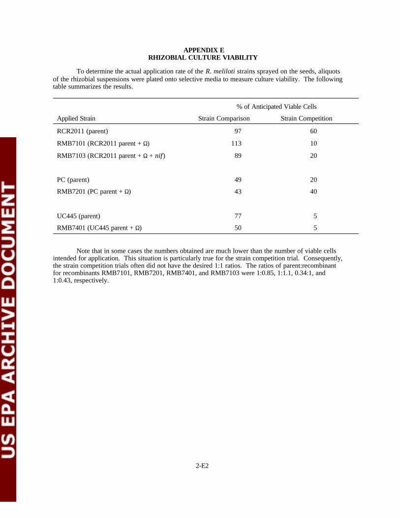
APPENDIX ERHIZOBIAL CULTURE VIABILITY
To determine the actual application rate of the R. meliloti strains sprayed on the seeds, aliquots of the rhizobial suspensions were plated onto selective media to measure culture viability. The following table summarizes the results.
% of Anticipated Viable Cells
Applied Strain Strain Comparison Strain Competition
RCR2011 (parent)
RMB7101 (RCR2011 parent + S)
RMB7103 (RCR2011 parent + S + nif)
PC (parent)
RMB7201 (PC parent + S)
UC445 (parent)
RMB7401 (UC445 parent + S)
97 60
113 10
89 20
49 20
43 40
77 5
50 5
Note that in some cases the numbers obtained are much lower than the number of viable cells intended for application. This situation is particularly true for the strain competition trial. Consequently, the strain competition trials often did not have the desired 1:1 ratios. The ratios of parent:recombinant for recombinants RMB7101, RMB7201, RMB7401, and RMB7103 were 1:0.85, 1:1.1, 0.34:1, and 1:0.43, respectively.
2-E2

APPENDIX F
ALFALFA YIELDS IN THE FIELD TESTS
2-F1
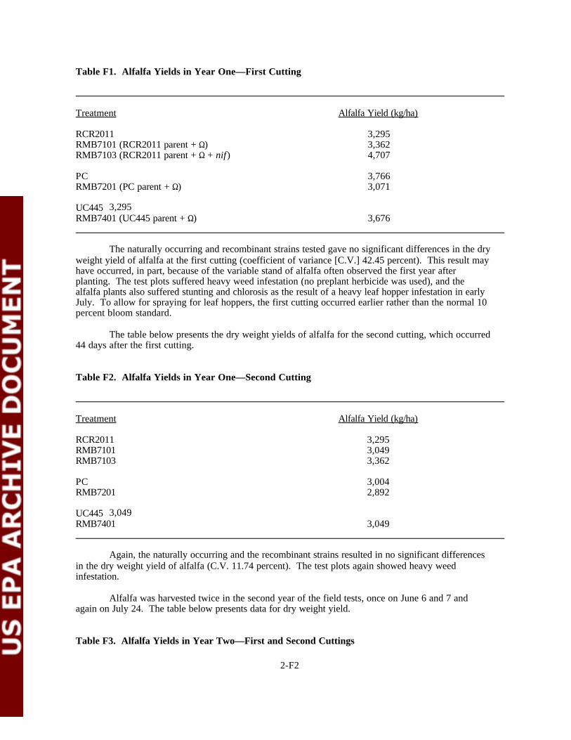
Table F1. Alfalfa Yields in Year One—First Cutting
Treatment
RCR2011RMB7101 (RCR2011 parent + S)RMB7103 (RCR2011 parent + S + nif)
PCRMB7201 (PC parent + S)
UC445 3,295RMB7401 (UC445 parent + S)
Alfalfa Yield (kg/ha)
3,295 3,362 4,707
3,766 3,071
3,676
The naturally occurring and recombinant strains tested gave no significant differences in the dry weight yield of alfalfa at the first cutting (coefficient of variance [C.V.] 42.45 percent). This result may have occurred, in part, because of the variable stand of alfalfa often observed the first year after planting. The test plots suffered heavy weed infestation (no preplant herbicide was used), and the alfalfa plants also suffered stunting and chlorosis as the result of a heavy leaf hopper infestation in early July. To allow for spraying for leaf hoppers, the first cutting occurred earlier rather than the normal 10 percent bloom standard.
The table below presents the dry weight yields of alfalfa for the second cutting, which occurred 44 days after the first cutting.
Table F2. Alfalfa Yields in Year One—Second Cutting
Treatment
RCR2011 RMB7101 RMB7103
PC RMB7201
UC445 3,049 RMB7401
Alfalfa Yield (kg/ha)
3,295 3,049 3,362
3,004 2,892
3,049
Again, the naturally occurring and the recombinant strains resulted in no significant differences in the dry weight yield of alfalfa (C.V. 11.74 percent). The test plots again showed heavy weed infestation.
Alfalfa was harvested twice in the second year of the field tests, once on June 6 and 7 and again on July 24. The table below presents data for dry weight yield.
Table F3. Alfalfa Yields in Year Two—First and Second Cuttings
2-F2

Treatment
RCR2011 RMB7101 RMB7103
PC RMB7201
UC445 4,304 RMB7401 C.V. (%)
Alfalfa Yield (kg/ha) 1st Cutting 2nd Cutting
4,304 6,052 4,102 6,232 4,416 6,590
4,281 6,254 4,506 6,590
6,209 4,438 6,276 11.50 6.95
The second year of the strain comparison test showed no significant differences in alfalfa dry weight yield with wild-type and recombinant R. meliloti strains. The second year's alfalfa growth lacked much of the variation seen in the first year. Consistent trends, however, were not evident.
The field data showed no conclusive trends toward either increased or decreased growth of alfalfa as compared with the parent strains. Therefore, the field tests indicate that the recombinant rhizobia posed little risk of decreasing alfalfa yields. The greenhouse data, although faulty, also indicated little potential for decreased growth of alfalfa from the GEMs.
2-F3

SECTION THREE
ECOLOGICAL RISK ASSESSMENT CASE STUDY:
EFFECTS OF RADIONUCLIDES IN THE COLUMBIA RIVER SYSTEM— A HISTORICAL ASSESSMENT

AUTHORS AND REVIEWERS
AUTHORS
Stephen L. FriantEnvironmental Science DepartmentBatelle Pacific Northwest LaboratoriesRichland, WA
Charles A. BrandtEnvironmental Science DepartmentBatelle Pacific Northwest LaboratoriesRichland, WA
REVIEWERS
Thomas Sibley (Lead Reviewer)Fisheries Research InstituteUniversity of WashingtonSeattle, WA
Gregory R. BiddingerExxon Biomedical Sciences, Inc.East Millstone, NJ
Joel S. Brown University of Illinois
at Chicago Chicago, IL
Herbert GroverBenchmark Environmental CorporationAlbuquerque, NM
Joseph E. LepoCenter for Environmental Diagnostics
and BioremediationUniversity of West FloridaGulf Breeze, FL
Frieda B. TaubSchool of FisheriesUniversity of WashingtonSeattle, WA
3-2

CONTENTS
ABSTRACT . . . . . . . . . . . . . . . . . . . . . . . . . . . . . . . . . . . . . . . . . . . . . . . . . . . . . . . . . . . . . . . 3-7
3.1. RISK ASSESSMENT APPROACH . . . . . . . . . . . . . . . . . . . . . . . . . . . . . . . . . . . . . . . . . . . 3-8
3.2. STATUTORY AND REGULATORY BACKGROUND . . . . . . . . . . . . . . . . . . . . . . . . . . . . . . 3-8
3.3. CASE STUDY DESCRIPTION . . . . . . . . . . . . . . . . . . . . . . . . . . . . . . . . . . . . . . . . . . . . . 3-10
3.3.1. Background Information and Objective . . . . . . . . . . . . . . . . . . . . . . . . . . . . . . . . . . 3-103.3.2. Problem Formulation . . . . . . . . . . . . . . . . . . . . . . . . . . . . . . . . . . . . . . . . . . . . . . . 3-12
3.3.2.1. Stressors . . . . . . . . . . . . . . . . . . . . . . . . . . . . . . . . . . . . . . . . . . . . . . 3-123.3.2.2. Biological Fate of Radionuclides . . . . . . . . . . . . . . . . . . . . . . . . . . . . . . . 3-143.3.2.3. Ecosystem Potentially at Risk . . . . . . . . . . . . . . . . . . . . . . . . . . . . . . . . 3-153.3.2.4. Endpoint Selection . . . . . . . . . . . . . . . . . . . . . . . . . . . . . . . . . . . . . . . . 3-153.3.2.5 Conceptual Model . . . . . . . . . . . . . . . . . . . . . . . . . . . . . . . . . . . . . . . . 3-15
3.3.3. Analysis: Characterization of Exposure . . . . . . . . . . . . . . . . . . . . . . . . . . . . . . . . . 3-17
3.3.3.1. Sample Location . . . . . . . . . . . . . . . . . . . . . . . . . . . . . . . . . . . . . . . . . 3-173.3.3.2. Data Analysis . . . . . . . . . . . . . . . . . . . . . . . . . . . . . . . . . . . . . . . . . . . 3-183.3.3.3. Exposure From Measured River Water Concentrations . . . . . . . . . . . . . . . 3-183.3.3.4. Calculation of Organism Dose . . . . . . . . . . . . . . . . . . . . . . . . . . . . . . . . 3-183.3.3.5. Dose From Water Exposure . . . . . . . . . . . . . . . . . . . . . . . . . . . . . . . . . 3-233.3.3.6. Dose From Measured Tissue Concentrations . . . . . . . . . . . . . . . . . . . . . 3-233.3.3.7. Dose From Measured Sediment Concentrations . . . . . . . . . . . . . . . . . . . . 3-27
3.3.4. Analysis: Characterization of Ecological Effects . . . . . . . . . . . . . . . . . . . . . . . . . . . 3-27
3.3.5. Risk Characterization . . . . . . . . . . . . . . . . . . . . . . . . . . . . . . . . . . . . . . . . . . . . . . 3-31
3.3.5.1. Acute Exposure to Ionizing Radiation . . . . . . . . . . . . . . . . . . . . . . . . . . 3-313.3.5.2. Chronic Exposure to Ionizing Radiation . . . . . . . . . . . . . . . . . . . . . . . . . 3-323.3.5.3. Uncertainty . . . . . . . . . . . . . . . . . . . . . . . . . . . . . . . . . . . . . . . . . . . . . 3-323.3.5.4. Conclusions . . . . . . . . . . . . . . . . . . . . . . . . . . . . . . . . . . . . . . . . . . . . 3-33
3.4. REFERENCES . . . . . . . . . . . . . . . . . . . . . . . . . . . . . . . . . . . . . . . . . . . . . . . . . . . . . . . . 3-36
3.5. ADDITIONAL READING . . . . . . . . . . . . . . . . . . . . . . . . . . . . . . . . . . . . . . . . . . . . . . . . 3-39
APPENDIX A—COLUMBIA RIVER FISH SPECIES AND FOOD WEB . . . . . . . . . . . . . . . . . . . . 3-A1
APPENDIX B—CRITR2 CODE CALCULATIONS ANDBIOACCUMULATION FACTORS . . . . . . . . . . . . . . . . . . . . . . . . . . . . . . . . . . . . . . 3
3-3
LIST OF FIGURES
Figure 3-1. Structure of assessment for effects of radionuclides . . . . . . . . . . . . . . . . . . . . . . . 3-9
Figure 3-2. Location of the Hanford Reach of the Columbia River . . . . . . . . . . . . . . . . . . . . . 3-11
Figure 3-3. Monthly concentrations for selected radionuclides in Columbia River grabsamples, 1963 . . . . . . . . . . . . . . . . . . . . . . . . . . . . . . . . . . . . . . . . . . . . . . . . . 3-20
Figure 3-4. Monthly concentrations for selected radionuclides in Columbia River grab samples, 1964 . . . . . . . . . . . . . . . . . . . . . . . . . . . . . . . . . . . . . . . . . . . . . . . . . 3-21
Figure 3-5. Ranges of sensitivities of aquatic organisms to acute radiation exposure . . . . . . . . . 3-29
Figure 3-6. Range of sensitivities of the early developmental stages of fish to acuteexposures . . . . . . . . . . . . . . . . . . . . . . . . . . . . . . . . . . . . . . . . . . . . . . . . . . . . 3-30
LIST OF TABLES
Table 3-1. Summary of Water Quality Data, 1957-1973 . . . . . . . . . . . . . . . . . . . . . . . . . . . . 3-12
Table 3-2. Water Sampling Matrix (1963-1964) . . . . . . . . . . . . . . . . . . . . . . . . . . . . . . . . . 3-17
Table 3-3. Maximum Grab Sample Water Exposure Concentrations for 1963-1964 Time Period . . . . . . . . . . . . . . . . . . . . . . . . . . . . . . . . . . . . . . . . . . . . . . . . . . . . . . . 3-20
Table 3-4. CRITR2 Code Calculation of Organism Dose From Water Exposure to Various Radionuclides . . . . . . . . . . . . . . . . . . . . . . . . . . . . . . . . . . . . . . . . . . . 3-22
Table 3-5. Calculated Dose Based on Tissue Concentration for Selected Organisms of theColumbia River . . . . . . . . . . . . . . . . . . . . . . . . . . . . . . . . . . . . . . . . . . . . . . . . 3-24
Table 3-6. Maximum Sediment Radionuclide Concentrations in the Hanford Reach and Dose to an Organism Living in the Sediments . . . . . . . . . . . . . . . . . . . . . . . . . . . 3-26
Table 3-7. Hazard Quotient for Early Development Stage of Fish and Adult Fish . . . . . . . . . . . 3-30
LIST OF COMMENT BOXES
Comments on Problem Formulation . . . . . . . . . . . . . . . . . . . . . . . . . . . . . . . . . . . . . . . . . . . . . . 3-17
Comments on Characterization of Exposure . . . . . . . . . . . . . . . . . . . . . . . . . . . . . . . . . . . . . . . . 3-27
Commands on Characterization of Ecological Effects . . . . . . . . . . . . . . . . . . . . . . . . . . . . . . . . . . 3-31
Comments on Risk Characterization . . . . . . . . . . . . . . . . . . . . . . . . . . . . . . . . . . . . . . . . . . . . . . 3-34
3-4

LIST OF ACRONYMS
BCF bioconcentration factor
CERCLA Comprehensive Environmental Response, Compensation, and Liability Act of 1980
DOE Department of Energy
HQ hazard quotient
NRDA Natural Resource Damage Assessment
PNL Pacific Northwest Laboratory
RM River Mile
USGS United States Geological Survey
3-5

ABSTRACT
In 1943, nuclear production activities began at the U.S. Department of Energy's (DOE) Hanford site in south-central Washington State. These activities continued for many years. During this time, the site discharged radioactive effluents into the Columbia River, which runs through the northern portion of the site and borders it on the east (the Hanford Reach). The DOE requested the Pacific Northwest Laboratory (PNL) to conduct an ecological risk assessment to determine whether the ecological risk assessment framework (EPA, 1992) used for hazardous chemicals is applicable to radionuclides as stressors. PNL conducted this ecological risk assessment using historical Hanford site monitoring data, which had been collected to characterize human dose. The data characterized exposure by measuring radioactivity in water, sediments, and biota. The data used in the current investigation were collected during 1963-1964, a period of peak production of nuclear material. During this time, the maximum number of eight reactors were operational.
PNL employed two approaches in assessing ecological risk to Columbia River organisms. The first approach used environmental exposure data (water concentrations for radionuclides) to calculate dose to a variety of aquatic organisms, including the most sensitive receptors (fish). The second approach made use of measured tissue concentrations of selected aquatic organisms to calculate organism internal dose.
PNL used dose to assess potential toxic effects and assess regulatory compliance. Risk characterization was developed by comparing dose levels in fish and other organisms found in the Columbia River to known effect concentrations through a hazard quotient for acute dose and possible developmental effects. The assessment endpoint was protection of fishes in the Columbia River, and the measurement endpoint was increases in mortality and sublethal effects. One of the most sensitive ecological receptors was the early developmental stage of chinook salmon.
The major conclusions of the study are:
# The ecological risk assessment paradigm is applicable to radionuclides as well as to hazardous chemicals, as evidenced from the exposure, effect, and risk characterization.
# The most sensitive life stage of fish (i.e., salmon embryo) did not appear to be at risk from radionuclide exposure in sediments or water.
# During peak production at Hanford, releases of radionuclides did not result in any measurable risk to the Columbia River ecosystem, as evidenced by indicator species and regulatory benchmarks.
# Dose rates to Columbia River animals during the study period did not exceed the DOE standard of 1 rad/d per DOE Order 5400.5 (DOE, 1989). Based on the computer code CRITR2, only crayfish and a plant-eating duck received a dose rate exceeding 1 rad/d. However, this risk assessment did not include ducks, and the actual calculation of dose to crayfish from whole organism counts gave values considerably less than both the modeled dose and 1 rad/d.
3-6

3.1. RISK ASSESSMENT APPROACH
The ecological risk assessment follows the sequence of the U.S. Environmental Protection Agency's Framework for Ecological Risk Assessment (EPA, 1992). This arrangement includes problem formulation, analysis, and risk characterization, respectively (figure 3-1).
Exposure of aquatic organisms to radioactivity can elicit a toxic response depending on the organism, level of dose, type of radionuclide, and habitat requirements of the exposed organism. In this study, the assessment endpoint was defined as the maintenance of important recreational and commercial fish populations in the Columbia River. The measurement endpoint from radioactive dose was toxicological response. This assessment did not consider elemental chemical toxicity of each radionuclide.
The major ecological components are benthic macroinvertebrates, zooplankton, phytoplankton, and fish of the Columbia River. Fish species in the Columbia River are important commercial, recreational, cultural, and regional assets.
Data analysis included exposure and effects characterization. Exposure characterization consisted of an assessment of radioactivity at several river stations downstream from the Hanford site. Measured river activity was used to calculate ionizing radiation dose from water to selected organisms using bioaccumulation factors and computer modeling. A second and more direct means of estimating dose to aquatic organisms used measured fish tissue concentrations. Available sampling data included sediments, water, and biota.
Characterization of effects to aquatic organisms entailed using available toxicity data and regulatory standards. The characterization was conducted at the individual level, qualitatively interpreted, and applied to the population level of ecological organization. Risk characterization was based on a hazard quotient (HQ), defined as the ratio of radionuclide organism dose (exposure or tissue value) to benchmark dose values.
3.2. STATUTORY AND REGULATORY BACKGROUND
Although federal regulations do not require quantitative ecological risk assessments, they can be used effectively to support regulatory requirements under nearly all of the major federal environmental statutes (e.g., the Comprehensive Environmental Response, Compensation, and Liability Act, CERCLA). Other potential applications include supporting compliance with federal Executive Orders and with policy directives of various government agencies (e.g., DOE Orders).
A number of federal statutes have promulgated risk-based and technology-based standards for the protection of ecological resources (e.g., water quality criteria under the Clean Water Act). However, only one standard has been published for the protection of ecological resources from exposure to radioactive materials. DOE Order 5400.5 (DOE, 1989) stipulates that the interim dose limit for native aquatic animal organisms "shall not exceed 1 rad per day from exposure to the radioactive material in liquid wastes discharged to natural waterways."
3-7


3.3. CASE STUDY DESCRIPTION
3.3.1. Background Information and Objective
It is generally assumed that human health risk standards for radionuclides protect wildlife sufficiently. However, under some circumstances the risk to wildlife from radionuclides may need to be considered, such as managing risks, developing cleanup strategies, and identifying injury under the Natural Resource Damage Assessment (NRDA) process. The objective of this case study is to evaluate the applicability of the ecological risk assessment paradigm for radionuclides as stressors in the Columbia River.
The Hanford site, an area of slightly more than 1,400 km2 (560 mi2), straddles the Columbia River just north of Richland, Washington. Three northwest-southeast-trending basalt ridges cross this broad, relatively level gravel plain. The semiarid climate supports various communities of shrubs—steppe and grassland.
The Columbia River extends 1,954 km (1,214 mi) from its origin in Columbia Lake in British Columbia to its mouth at Astoria, Oregon, making it the fourth-longest river in North America. Typical flow rates of the Columbia River at Priest Rapids Dam range from 2,800 to 3,400 cubic meters per second (cms), or 99,000 to 122,000 cubic feet per second (cfs) (Woodruff et al., 1991).
The Columbia River has eight primary uses:
1. River navigation through navigation locks from the Pacific Ocean to the Port of Benton in Richland.
2. Agricultural purposes, primarily irrigation. Approximately 6 percent of the Columbia Basin's water is diverted for agricultural use.
3. Nonagricultural irrigation. 4. Electric power generation, provided by the system of 11 dams along the Columbia River in
the United States. 5. Flood control, also provided by the dams. 6. Fish and wildlife habitat, especially for anadromous salmon. The Hanford Reach comprises
the last major salmon and steelhead spawning area within the Columbia River proper. The Columbia River also supports the vast majority of mesic terrestrial habitat in the semiarid Hanford Reach.
7. Water supplies to numerous municipalities and industries. 8. Recreational use.
The Hanford Reach of the Columbia River runs from Priest Rapids Dam to just north of the City of Richland and flows past the reactor areas of the Hanford site (figure 3-2). The average annual flow of the Columbia River in the Hanford Reach, based on 65 years of record, is about 3,400 cms (120,100 cfs) (DOE, 1988). Flows in the Hanford Reach vary widely, not only because of the annual flood flow but also because of daily regulation by the upstream power-producing Priest Rapids Dam. Flow rates during the late summer, fall, and winter may vary from a low of 1,100 cms (36,000 cfs) to as much as 4,800 cms (160,000 cfs) each day. During the spring runoff, peak flow rates from 4,800 to 20,000 cms (160,000 to 650,000 cfs) can occur.
3-9


The Washington State Department of Ecology classifies the Columbia River water quality as Class A (excellent) between Grand Coulee Dam and the mouth of the Columbia River (DOE, 1988). Table 3-1 shows water quality data between Priest Rapids Dam and Pasco, Washington, for the years 1957-1973. The dominant physical feature of the Columbia River through the Hanford Reach is the high flow rate, which is subject to large, diurnal water-level fluctuations that change the shoreline configuration and expose gravel substrate and periphyton to alternate periods of wetting and drying. The Reach has a low level of suspended sediment, 1 to 7 mg/L.
The river-bottom sediments from Priest Rapids Dam to several kilometers below the confluence of the Snake and Columbia Rivers are primarily mixed sands and gravels with some cobbles (maximum diameter . 20 cm). Coarser sediments predominate from Priest Rapids Dam through the reactor areas (DOE, 1988). The streambed near Richland consists of sand in deep channels and a mixture of sand, silt, and some clay in shallow areas (DOE, 1988). Most of the Hanford-produced cationic radionuclides are associated with suspended particulates and subsequent fine sediments (Beasly and Jennings, 1984).
Because of the many dams on the Columbia River, the only free-flowing U.S. section occurs between Priest Rapids Dam (River Mile [RM] 397) and McNary Reservoir (RM 351). The Priest Rapids Dam immediately upstream from the Hanford site regulates flow. No significant tributaries enter the stream in this section, which lies mostly within the Hanford site.
The main channel of the Hanford Reach is braided around the island reaches and submerged rock ledges and gravel bars, causing repeated pooling and channeling. The riverbed material is mobile and dependent on river velocities; it typically is composed of sand, gravel, and rocks up to 20 cm (8 in) in diameter. Small fractions of silts and clays are associated with the sands in areas of low-velocity deposition.
3.3.2. Problem Formulation
3.3.2.1. Stressors
The release of radionuclides from Hanford operations is one of several possible stressors to the ecosystems of the Columbia River. Other possible stressors include thermal discharges from Hanford reactors; varying river levels because of dams; the physical barrier to fish migration from the dams; and heavy agricultural, commercial, and recreational activities along the river. However, this assessment concerns only radionuclides as stressors of concern.
The cooling effluents of Hanford reactors contain over 60 radionuclides. Becker (1990) has reported that during the period of maximum reactor production (mid-1960s), the Hanford site discharged over 300,000 curies per year to the river. Radioactive decay influenced the relative abundance of different radionuclides in the river (Becker, 1990). In fact, many of the radionuclides discharged by the Hanford site have a short half-life and were not detected in the effluent discharge. Others could not be detected in the river after dilution. Becker (1990)
3-11

Table 3-1. Summary of Water Quality Data, 1957-1973 (DOE, 1988)
Color Ortho Location/ DOa Temperature Coliform (PT-COa Hardness Turbidity PO4-P NO3-N Statistic (mg/L) (°C) (MPNa/100 mL) pH units) (mg/L) (JTUa) (mg/L) (mg/L)
Below Priest Rapids (River Mile 395)
Minimum 9.5 1.8 0 6.5 0 55 0 0.01 0.02
Mean 11.9 11.4 131 7.7 5 69 3 0.08 0.10
Maximum 15.9 19.2 2,000 8.5 33 81 29 0.15 1.50
Pasco (River Mile 330)
Minimum 6.8 3.0 1 6.8 0 40 0 0.01 0.05
Mean 10.8 12.2 182 8.1 8 73 15 0.10 0.19
Maximum 14.3 22.0 4,800 8.6 68 90 140 0.02 0.37
aDO = Dissolved oxygen. JTU = Jackson turbidity units. MPN = Most probable number. PT-CO = Platinum-cobalt.
3-12

identified three radionuclides as being of concern because of their potential biological significance: phosphorus-32, chromium-51, and zinc-65. Together they account for over 90 percent of potential radiological dose to aquatic organisms. All are nuclear activation products that are activated as Columbia River water cools the reactor core. The potential for some radionuclides to bioaccumulate in aquatic food webs causes concern with respect to both the human exposure pathways and potential ecosystem effects.
Among radionuclides, phosphorus-32 and zinc-65 are potential stressors because of their biological importance and fate: they are essential elements for organism growth and are incorporated into the aquatic food web. One study conducted in the Hanford Reach from 1961 to 1968 noted a seasonal pattern of uptake by algae, with higher radioactivity in winter and lower in summer (Becker, 1990). This pattern reflects concentration and dilution phenomena from river flows.
Unlike phosphorus-32 and zinc-65, chromium-51 is not considered a major biological hazard. This radionuclide has a short half-life, low biological mobility (i.e., it has no known essential role in the physiology of organisms), and weak radiations. It does not accumulate to any extent in aquatic organisms and is transported with river-suspended particulate material with little dissolution (Becker, 1990). However, the risk assessment included it because it was a significant activation product.
The half-lives of the three radionuclides considered in the risk assessment are:
# Phosphorus-32: 14.2 days # Chromium-51: 27.8 days # Zinc-65: 245.0 days
Phosphorus-32 is a beta emitter (negatrons); chromium-51 emits gamma radiation and electrons; and zinc-65 is primarily a gamma emitter, but also emits positrons and electrons.
3.3.2.2. Biological Fate of Radionuclides
Phosphorus, including phosphorus-32, is a building block of various tissues and is a key element in many biochemical transformations, especially energy transduction (ATP, ADP, GTP, etc.). The element is comparatively scarce in the environment. Organisms can concentrate phosphorus, including phosphorus-32, to levels that greatly exceed the concentration in the ambient media. Phosphorus has a bioconcentration factor (BCF) of 24,000 for freshwater plants and 8,000 for freshwater animals (Becker, 1990).
Terrestrial plants take up little chromium-51 from soils, <0.5 percent (Becker, 1990). In aquatic systems, this element sorbs to particulate material and is transported along with it. Becker (1990) reported that in biological systems chromium-51 has an affinity for the blood of fish.
Organisms accumulate a measurable fraction of zinc-65. In aquatic systems, this radionuclide is transported through aquatic food webs. With chronic uptake, substantial tissue accumulation can occur. In the Pacific Ocean, Becker (1990) noted BCFs of up to 103 for algae and 105 for certain molluscs. The BCF for plankton in the Columbia River ranges from 300 to 19,000 (Cushing and Watson, 1966; Cushing, 1967a, b), with adsorption as the primary means of uptake. Because of its long half-life and biological mobility, zinc-65 can be transported through food webs.
3.3.2.3. Ecosystem Potentially at Risk
The Columbia River supports a diversity of aquatic and terrestrial wildlife. The major ecological components are benthic macroinvertebrates, zooplankton, phytoplankton, and fish. Although a detailed description of the wildlife exceeds the scope of this effort, appendix A lists the fish species and shows the generalized aquatic food web. This risk assessment focuses on the fish of the Columbia River because they are aquatic organisms sensitive to ionizing radiation and because the Columbia River
3-13

supports a wide variety of fish, including several species that are commercial, recreational, and cultural assets of the region.
3.3.2.4. Endpoint Selection
Exposure of aquatic organisms to radioactivity can elicit a toxic response depending on the dose level, the length of exposure, the particular species, and the life stage at the time of exposure. The magnitude of the response is proportional to radiological dose. In this study, the assessment endpoint was the health and condition of local populations of selected fish species that were of commercial, recreational, and cultural interest.
The risk assessment evaluated multiple measurement endpoints. They included literature investigations of adverse effects on fish, such as acute mortality and sublethal and developmental effects. Dose from ionizing radiation was evaluated in the maximally exposed individual fish and fish in early developmental stages during the study period. Because no net increase occurred in the concentration of elements, the assessment considered only toxicity resulting from ionizing radiation, not toxicity resulting from chemical characteristics.
3.3.2.5. Conceptual Model
Radionuclides in the Columbia River are partitioned between river water, sediment, and the aquatic food web. Organisms become exposed through direct contact with river water, through contact or ingestion of contaminated sediments, or through food web incorporation of radionuclides.
Two organism exposure pathways exist for ionizing radiation. In the external exposure pathway, an organism receives a dose from its external environment, such as ionizing radiation from the water. If the energy of the radiation is high enough, it may penetrate the organism's external tissue. In the internal exposure pathway, an organism receives a dose of ionizing radiation as a result of uptake of a radionuclide. Consequently, exposure occurs to internal organs and tissues. The significance of each exposure pathway depends on the aquatic fate of the radionuclide, its concentration, the energy of its radiation, and also on the pathway of bioaccumulation.
The level of organism dose from either external or internal exposure depends on the length of time an organism spends in the Hanford Reach feeding and breeding habitats, the degree of interaction with the sediments (i.e., living on or in the sediments), the discharged levels of radionuclides, and the river flows. Potential dose to aquatic organisms equals the sum of the total ionizing radiation dose from multiple radionuclides.
Possible exposure scenarios include organisms living near or in reactor effluent discharges, at various locations downriver of Hanford, and on or in contaminated sediments. A resident fish, such as whitefish, can spend its entire life in the Hanford Reach. The adult chinook salmon, on the other hand, is present only during selected periods of the year.
Generally, higher-level organisms such as fish have greater sensitivity to ionizing radiation than lower-level organisms such as algae and invertebrates (Frank, 1973). Consequently, fish can serve as indicators or benchmarks of the health of fish populations and the ecosystem. For fish, sensitivity varies with developmental stage, (i.e., adult fish being less sensitive then juveniles), amount of time required for various developmental stages, and number of fertilized eggs produced (Whicker and Shultz, 1982). Species fecundity factors into extrapolating individual organism effects to a population. For example, species with high fecundity rates most likely will not experience adverse effects to the same degree as species with low fecundity rates. In addition, the exposure of organisms to low-level ionizing radiation can promote injury repair mechanisms.
For Hanford, most of the available monitoring data for radionuclides were for river water activity and tissue concentrations of selected species of fish, including mountain whitefish (Prosopium
3-14

williamsoni). One of the most fished species in the Columbia River, mountain whitefish remains resident throughout the year, making it a useful biomonitor of radionuclide incorporation into the human food chain. The food chain accumulation of radionuclides by whitefish occurs in a three step process:
Water 6 Algae 6 Insects 6 Whitefish
Calculated dose to whitefish can be extrapolated to other fish species, such as adult chinook salmon that occur seasonally in the Hanford Reach of the Columbia River. In the risk assessment, whitefish served as an indicator or "generic" fish to develop a potential exposure/dose scenario. Where available, the risk assessment incorporated data for other fish species along with supportive or ecosystem descriptive data for phytoplankton, snails, and crayfish. Dose was estimated from exposure to measured radionuclides in the river to salmon embryos, identified as one of the most sensitive organisms to ionizing radiation.
Comments on Problem Formulation
Strengths of the case study include:
! This case study was well written and well organized. application of the EPA Risk Assessment Framework because discrete stressors are easily identified and measured and substantial data are available on their biological impacts. fit nicely into the risk assessment paradigm.
Limitations include:
! Because the Columbia River ecosystem has been affected by many other factors, radiation may have a relatively small impact on salmon. may be valid to restrict the risk assessment to a single stressor that does not reflect the "real world" situation, other stressors on salmon should be identified.
It is an ideal case for the
Assessment and measurement endpoints are identified and
Therefore, although it
! The authors should point out that data were developed for the specific case study, rather than for a full-ranging risk assessment that could consider other stressors. problem or risk to the ecosystem is negligible.
! The total biological community is not well characterized.
DOE and EPA need to know whether radionuclides are a major
3.3.3. Analysis: Characterization of Exposure
Making use of the 1963-1964 data for sediments, water, and biota, the exposure characterization employed two approaches to evaluate dose, which provided independent assessments of dose. The first approach evaluated river radioactivity at several stations downstream of the Hanford site. This approach then modeled organism dose using biological accumulation factors for several "generic" aquatic organisms from measured radionuclide water concentrations during the study period, 1963-1964. The second approach used measured radionuclide tissue concentrations to calculate dose to whitefish. Directly measured tissue activity has the advantage of considering all environmental pathways: water and food uptake, excretion, sediments, etc. However, this approach has the disadvantage of measuring selected radionuclides only in fish muscle tissue. As a result, the approach reflects the human pathway and places less emphasis on effects to the fish. For example, although organs and bones also accumulate radionuclides, they were not included in the dose calculation.
3-15

3.3.3.1. Sample Location
The initial exposure characterization was limited to the Richland Station (RM 344), although ultimately all available data from the Hanford Reach were reviewed and considered. The U.S. Geological Survey (USGS, 1966) indicated that the river is vertically and horizontally mixed at this point. This approach was used because of the potential for large spatial and temporal variability of radionuclide concentrations upstream. This variability resulted from the discharge of eight production reactors with individual production schedules. Once established, the relationship between exposure and potential effects can be applied to upstream locations.
3.3.3.2. Data Analysis
The risk assessment reviewed three data sets to characterize exposure: measured radionuclide river concentrations, measured sediment concentrations, and measured fish tissue concentrations. The data were collected during routine monitoring of radionuclide concentrations in the Columbia River system. River water was collected as composite, grab, or cumulative samples. The sampling scheme varied over the 2-year period (table 3-2). Figures 3-3 and 3-4 show the monthly water grab sample concentrations for selected radionuclides over the 2-year period. Water concentrations were generally highest during the winter and late fall and lowest in the spring and summer.
3.3.3.3. Exposure From Measured River Water Concentrations
Exposure concentrations were established by reviewing measured river activity data to determine the relationships among composite, grab, and continuous samples: that is, to see whether one form of sampling yielded consistently higher water concentrations than another. The results of this analysis showed that the highest river concentrations of radionuclides occurred in whole-water grab samples.
An upper-boundary exposure concentration was derived by using the maximum observed grab sample water concentration for the 2-year study period for each radionuclide shown in table 3-3. These concentrations were assumed to represent the maximum concentration for exposure of river organisms. If the effect characterization indicated a potential risk, then more typical exposure concentration scenarios could be developed.
The maximum sediment concentration measured for each radionuclide was used to calculate organism dose.
3-16

Dec
o
*
Nov
x
x
o
*
Oct
Table 3-2. Water Sampling Matrix (1963-1964) (Dirkes, 1992; Haushild et al., 1966; Nelson et al., 1964)
Frequencya
Station
x
x
x
o
*
Sep
x
x
o
*
Aug
x
x
x
o
*
*
o
o
Jul
x
x
x
o
*
*
o
o
Jun
x
x
o
*
*
o
o
May
x
x
x
o
*
o
o
Apr
x
x
o
*
o
o
Mar
x
x
o
*
o
o
Feb
xb
x
x
o
*
o
o
aTotals for 1963: Grab--159. Totals for 1964: Grab--149.
Comp--194. Cum --300.
bLegend: x--every 2 weeks. o--weekly. *--monthly.
Jan
x
x
o
*
o
o
Comp
Comp
Type
Grab
Grab
Grab
Grab
Cum
Cum
Location
Richland
Richland
Hanford
Hanford
1963
1964
3-17
x
x


Table 3-3. Maximum Grab Sample Water Exposure Concentrations for 1963-1964 Time Period (Dirkes, 1992; Nelson et al., 1964)
Radionuclide Concentration (pCi/L)
As-76 2,300
Co-60 120
Cr-51 25,000
Cu-64 10,000
I-131 34
Na-24 5,600
Np-239 5,600
P-32 630
RE+Y 1,400
Sr-90 2.6
Zn-65 1,800
(3-1)
(3-2)
3.3.3.4.
The internal total-body dose rate to an organism from water exposure for a number (N) of radionuclides is given as:
where Rc is the dose rate to total body of organism c (rad d-1), bi,c is the specific body burden of nuclide i in organism c (Bq kg-1), and Ei,c is the effective absorbed energy rate for nuclide i per unit activity in organism c (rad Ci-1 d-1):
Ei,c = ,i,cMeV dis-1 × 3.70E10 dis s-1 Ci-1
86,400 sd-1 × 1.602E-11 rad-1 MeV = 5.12E4 ,i,c
(where , is the effective absorbed energy for nuclide i in organism c).
For a primary organism:
where Ci,c is the concentration of nuclide i in the water to which organism c is exposed (Bq m-3) and Bi,c is the bioaccumulation factor for nuclide i and organism c (m3 kg-1).
Calculation of Organism Dose
Here the water concentration
3-20

(3-3)
already has been corrected for dilution and radioactive decay during transit from the point of release into the receiving water body to the region of the organism's habitat.
Combining equations 3-1 and 3-2 yields the dose rate in rad/d to the primary organism, as shown in equation 3-3 below. equations 3-1 and 3-2, except the radionuclide-specific BCF is not used and correction for decay and dilution is unnecessary.
For a secondary organism, such as an herbivore or carnivore, an expression can be written for a single radionuclide equating the change in body burden to the uptake and removal of the radionuclide.
3.3.3.5.
Table 3-4 shows the CRITR2 code calculations of organism dose from water exposure to various radionuclides. bioaccumulation factors used. Table 3-4 indicates internal dose, immersion or surface dose (external water dose), and sediment dose. Internal exposure gave the maximum dose. contributions, they were not considered in the risk characterization.
Table 3-4 summarizes dose for each organism. fish, crayfish, and ducks that eat plants and fish (DUCK-P and DUCK-F, respectively). ducks had the maximum dose rate, followed by plants, crayfish, fish, and fish-eating ducks. rates to the plant-eating duck and crayfish exceeded the 1 rad/d level. a dose rate of 0.42 rad/d.
The dose to salmon eggs was estimated from measured river water radionuclide activities (table 3-3). for developing plaice (Pleuronectes platessa) embryos with respect to various fission product radionuclides (Woodhead, 1970). from <1 to 10 as a function of the radionuclide. of 10 for all radionuclides shown in table 3-3. mm.
3.3.3.6.
Table 3-5 the Columbia River. (shell) at 0.39 rad/d and caddisfly at 0.38 rad/d. 0.73 rad/d. observed for whitefish during 1963-1964. highest body dose for the study period. concentrations and therefore underestimated whole-body burdens. adjusted these values to whole-body values. correction factors between whole body and muscle were 9:1 for phosphorus-32 and chromium-51 and 4:1 for zinc-65 (Poston and Strenge, 1989; U.S.
The calculation of internal dose from tissue concentration is the same as
Dose From Water Exposure
Appendix B provides a more detailed listing of CRITR2 code calculations and Water concentrations were maximum values for the 2-year period.
Since immersion and sediment doses made only minor
CRITR2 default organisms are generic plants, Plant-eating
The dose The maximally exposed fish had
Bioconcentration factors were estimated for salmon embryos from bioconcentration data reported
Concentration factors for day 4 of embryonic development ranged This assessment used a whole egg concentration factor
Dose calculations employed an overall egg diameter of 2 Dose to whole eggs was 0.00442 rad/d.
Dose From Measured Tissue Concentrations
lists calculated dose from measured tissue concentrations to selected organisms in Phytoplankton had the highest dose at 14 rad/d, followed by limpet hard parts
The maximally exposed fish dose was calculated to be For fish, table 3-5 concentrations used to calculate dose represent the maximum values
Dose was evaluated for other species, but whitefish had the Unfortunately, most of the fish data were muscle tissue
Consequently, the assessment Based on limited Hanford data and published literature, the
3-21
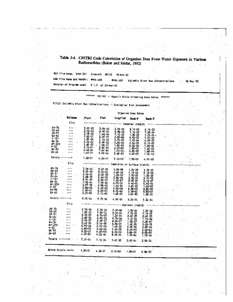


14.8 0.80
TotalP-32
23,000 0.21
20,700 1.7E-3 0.73
Calculated Dose Based on Tissue Concentration for Selected Organisms of the Columbia Rivera
La-140
4.4E-3
2.6E-3
4.0E-3
1.7E-3
1.8E-4
4.5E-4
5.900 0.021
Tissue Concentration (pCi/g wet weight)
113 9.7E-4
113 9.7E-4
73 4.2E-3
47 1.6E-3
12 1.2E-3
5 6.5E-4
14,000 0.70
3.1E-3
Zn-65
2,980 0.058
2,820 0.031
1,100 0.022
658 0.015
658 0.015
441 2.6E-3
811 5.1E-3
270 Dose, rad/d
102,000 13.1
Cu-64
8,560 0.29
2,230 0.076
4,500 0.076
2,230 0.35
3,320 0.025
383 0.028
48 0.044
291,000 6.8E-3
Mn-56
6,490 1.6E-4
1,700 2.2E-4
2,230 2.2E-4
7,480 1.2E-4
556 7.0E-5
617 2.1E-5
982 6.1E-5
59,500 5.2E-2
Cr-51
1,390 0.028
1,940 0.058
1,940 0.050
1,080 0.024
620 0.014
181 5.0E-3
536 0.035
aUsing minimum effective radius of 1.4 cm.
Na-24
1,414 Dose, rad/d
1,595 Dose, rad/d
1,595 Dose, rad/d
764 Dose, rad/d
644 Dose, rad/d
393 rad/d
136 Dose, rad/d
955 Dose, rad/d
Limpets (soft parts)
Clams (soft parts)
Fish (whitefish)
Limpets (shell)
Chironimids
Clam (shell)
Organism
Caddisfly
Table 3-5.
Plankton
Crayfish
3-24
0.38
0.15
0.17
0.39
0.065
0.036
0.085
0.73

Table 3-6. Maximum Sediment Radionuclide Concentrations in the Hanford Reach and Dose to an Organism Living in the Sediments (Dirkes, 1992; Haushild et al., 1966; Nelson et al., 1964)
Nuclide Concentration (pCi/Kg dry weight)a
Cr-51 13,000
Co-60 100
Sc-46 46
Zn-65 3,900
aTotal dose: Organism buried in sediment—0.16 rad/d. Organism on surface of sediment—0.08 rad/d.
Congress, Joint Committee on Atomic Energy, 1959). This correction introduces uncertainty into the effects characterization, but uncorrected muscle values could underestimate individual dose.
3.3.3.7. Dose From Measured Sediment Concentrations
Table 3-6 shows the calculated dose from exposure to radioactivity reported in sediments of the Columbia River. The calculated dose was quite small compared with other pathways.
Comments on Characterization of Exposure
Strengths of the case study include:
! The ability to evaluate the worst case (maximally exposed individual) at the most sensitive life stage is an efficient method of screening for population-level effects. collected on site.
Limitations include:
! Analysis also should consider potential uptake from food rather than only exposure or direct uptake from the water. suggest that activity in water cannot reliably predict exposure.
This study also benefits from the availability of long-term data sets
Large variance in BCF values
! In the computer model scenario, algae, crayfish, and fish were not growing or eating and did not accumulate a food chain dose. included ducks, they were not included in the ecological risk assessment because of limited data and limited ability to verify the model estimate.
Although the computer code
3.3.4. Analysis: Characterization of Ecological Effects
Characterization of effects was based on dose-response information for fish from available toxicity data and also on regulatory standards. Conducted at the individual level, the characterization was interpreted qualitatively and applied to the population level of ecological organization.
3-25

The general response of aquatic organisms to ionizing radiation occurs at both the cellular and biochemical levels. Environmental factors also can affect the level of response. An NCRP (1991) report, Effects of Ionizing Radiation on Aquatic Organisms, provided the basis for stressor-response relationships developed in this report. Figures 3-5 and 3-6 were adapted from the NCRP report and summarize the information on acute effects of ionizing radiation on aquatic organisms.
One would expect different fish species to accumulate different concentrations of radionuclides based on their feedings habits, age, length of time spent at the site, and other factors. Depending on the level of exposure, mortality can occur. The threshold level of radiation dose that can cause acute mortality occurs at approximately 100 rad (1 Gy) for amphibians and 1,000 rad (10 Gy) for crustaceans and fish (figure 3-5). Figure 3-5 summarizes the relationship between organism dose and response and also shows the range for LD50s. Under no circumstances did calculated dose to fish or other organisms exceed the boundary dose where acute effects would be observed. Dose calculations based on tissue concentrations for selected Columbia River organisms confirmed this finding. No aquatic animal organism used in the risk assessment exceeded the DOE dose limit of 1 rad/d.
Few studies have evaluated the effects of chronic exposure to ionizing radiation. However, it is known that the early developmental stages of chinook salmon are especially sensitive to ionizing radiation. NCRP (1991) reported that exposure to 5.1 rad/d (51 mGy/d) for up to 69 days produced no increase in mortality to chinook salmon embryos and alevins up to release as smolts. Hershberger et al. (1978) reported lower return of spawning adult chinook salmon after exposure of eggs and alevins at approximately 10 rad/d of gamma radiation. Gonadal development was retarded in chinook salmon on exposure to 10 rad/d delivered to embryos (Bonham and Donaldson, 1972). Other laboratory research (Erickson, 1973) found that an exposure of 0.4 rad/d (4.0 mGy/d) reduced courting activity for male Poecilia reticulata exposed as embryos. Chronic gamma radiation (190 days at an exposure of 18.5 rad/d) causes sterility in young adult Ameca splendens (Rackham and Woodhead, 1984).
Based on available literature, the dose used in DOE Order 5400.5 appears sufficiently conservative to protect most aquatic organisms. Consequently, unless future data indicate otherwise, this dose can be considered protective of populations and the ecosystem in general. To date, the sole qualifier is the work of Erickson (1973), who reported reduced male guppy courting activity when exposed to 0.4 rad/d. Little other information exists with regard to behavioral changes in fish exposed to ionizing radiation.
Figure 3-6 summarizes the effects of acute irradiation on development of fish. The threshold for developmental effects on fish occurs at approximately 5 rad (0.05 Gy), as observed for the one-cell-stage developing chinook salmon embryos. Radiosensitivity reportedly decreases
3-26


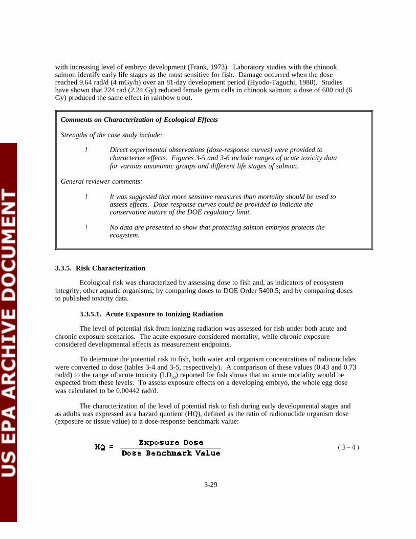
with increasing level of embryo development (Frank, 1973). Laboratory studies with the chinook salmon identify early life stages as the most sensitive for fish. Damage occurred when the dose reached 9.64 rad/d (4 mGy/h) over an 81-day development period (Hyodo-Taguchi, 1980). Studies have shown that 224 rad (2.24 Gy) reduced female germ cells in chinook salmon; a dose of 600 rad (6 Gy) produced the same effect in rainbow trout.
Comments on Characterization of Ecological Effects
Strengths of the case study include:
! Direct experimental observations (dose-response curves) were provided to characterize effects. Figures 3-5 and 3-6 include ranges of acute toxicity data for various taxonomic groups and different life stages of salmon.
General reviewer comments:
! It was suggested that more sensitive measures than mortality should be used to assess effects. Dose-response curves could be provided to indicate the conservative nature of the DOE regulatory limit.
! No data are presented to show that protecting salmon embryos protects the ecosystem.
(3-4)
3.3.5.
Ecological risk was characterized by assessing dose to fish and, as indicators of ecosystem integrity, other aquatic organisms; by comparing doses to DOE Order 5400.5; and by comparing doses to published toxicity data.
3.3.5.1.
The level of potential risk from ionizing radiation was assessed for fish under both acute and chronic exposure scenarios. considered developmental effects as measurement endpoints.
To determine the potential risk to fish, both water and organism concentrations of radionuclides were converted to dose (tables 3-4 and 3-5, respectively). rad/d) to the range of acute toxicity (LD50) reported for fish shows that no acute mortality would be expected from these levels. was calculated to be 0.00442 rad/d.
The characterization of the level of potential risk to fish during early developmental stages and as adults was expressed as a hazard quotient (HQ), defined as the ratio of radionuclide organism dose (exposure or tissue value) to a dose-response benchmark value:
Risk Characterization
Acute Exposure to Ionizing Radiation
The acute exposure considered mortality, while chronic exposure
A comparison of these values (0.43 and 0.73
To assess exposure effects on a developing embryo, the whole egg dose
3-29

If the HQ is equal to or greater than 1, the likelihood of an adverse effect or high risk exists. The characterization was completed for the maximally exposed individual for the study period. It was assumed that if risk to the individual was low, the population was not at risk.
The hazard quotients shown in table 3-7 for early developmental stages of fish and adults were compared with toxicity values and DOE Order 5400.5. The maximum hazard quotient was 0.73 for adult fish. Assuming that this was the maximally exposed individual, the likelihood of an adverse effect to an individual was low.
Table 3-7. Hazard Quotient for Early Development Stage of Fish and Adult Fish
Minimum Effect Maximum Exposure Level Hazard Quotient
Unfertilized ovum, One-cell stage 0.00442 0.96,a 0.4b 0.004,a 0.11b
Adult 0.73 1 0.73a,c
aBased on recommendation of the NCRP (1991).bBased on male courting activity in guppies (Erickson, 1973).cDOE Order 5400.5.
3.3.5.2. Chronic Exposure to Ionizing Radiation
Mortality from chronic exposure presented minimal risk to fish. Chronic exposure to 5.1 rad/d for up to 69 days did not produce any mortality to chinook salmon embryos or alevins (NCRP, 1991). Hershberger et al. (1978) reported lower return of spawning chinook salmon after exposure of eggs and alevins to 10 rad/d and effects on gonadal development in chinook salmon was reported to occur at 9.5 rad/d. Because the maximum dose rate to Columbia River adult fish and developing embryos was 0.73 and 0.00442 rad/d respectively, no chronic effects or mortality would be expected. Applying the behavior response noted for guppy embryo exposure (Erickson, 1973), the benchmark concentration would be 0.4 rad/d with an HQ of 0.1.
3.3.5.3. Uncertainty
Extrapolation of individual effects of radionuclides to populations and communities suffers from the same constraints as similar extrapolations for hazardous chemicals. The quantitative relationship between potential effects to fish or fish embryos and population and community response is not known. However, the effects data available for radionuclides showed that the single-cell stage in salmon is one of the more sensitive indicators of irradiation effects in fish and that protection of this stage of development should be protective of the population. Although specific data were not available for salmon embryo, data for embryo development of plaice was used to estimate dose.
The NCRP (1991) suggests that a "maximum dose rate 0.4 mGy/h (0.96 rad/d) would provide protection for endemic populations of aquatic organisms in environments receiving discharges of radioactive effluent." It further states, "adoption of a reference level of 0.4 mGy/h appears to represent a reasonable compromise based on current literature, i.e., considering both the nature of the effects observed at this dose rate and the limited amount of information on effects of radiation in natural populations, including interactions between ionizing radiation and ecological conditions." This value is also in agreement with DOE Order 5400.5.
Because whitefish are resident species in the Columbia River and can accumulate radionuclides throughout their life cycle, the assessment assumed that the whitefish tissue dose would be sufficiently
3-30

conservative to extrapolate dose levels to other adult fish, including salmon. Salmon, on the other hand, spend only a short period of time in the river and do not feed when present. In addition, during the spring and early fall when salmon are present, river concentrations of radionuclides were generally the lowest.
The risk characterization used the maximally exposed individual to calculate organism dose. The risk characterization assumed that if an organism dose is below any known effect level with some degree of certainty, then the likelihood of an adverse effect is minimal. (The assessment endpoint was maintenance of important recreational fish populations in the Columbia River measured by protection of fish populations and specifically salmon embryos.) Results indicate that this is a reasonable assumption. Fish appear to be a suitable choice of receptor for screening risk from ionizing radiation. In addition, a fish dose of less than 1 rad/d should be protective of the ecosystem in general. However, since CRITR2 indicate that ducks could have received a dose higher than 1 rad/d, further studies are warranted.
Another area of uncertainty in the risk assessment is the extrapolation of muscle tissue concentration to whole fish concentrations for radionuclides. The assumption that protection of the maximally exposed individual extrapolated to sensitive life stages constitutes an adequate measure of the assessment endpoint also is a source of uncertainty. Alternatively, the hazard quotient is a reasonable approach for radionuclides for baseline or screening assessments.
3.3.5.4. Conclusions
This study demonstrates that the ecological risk assessment paradigm is applicable to radioactive substances. However, stressor-response data were limited to acute exposures; few data addressed chronic sublethal exposures. Most endpoints used for hazardous chemicals are expected to be equally appropriate for radionuclides. This study uncovered only one benchmark that specifically addressed protecting aquatic organisms from exposure to radiation. DOE Order 5400.5 limits exposure to aquatic animals to 1 rad/d.
Risk characterization did not indicate any measurable risk to the most sensitive aquatic organism (early life stage of chinook salmon) from exposure to radionuclides in sediments or water in the Columbia River. During peak production at Hanford, releases of radionuclides to the river did not result in a dose to fish that would exceed those specified in DOE Order 5400.5.
Dose calculations for radionuclide exposure from water and tissue concentrations provide for two methods for assessing the potential risks. This study investigated both methods and found that both provided reasonable results for fish, algae, and crayfish. Areas of uncertainty included the relationship between muscle and whole fish concentrations, the lack of a strong data base for organism exposure to chronic radiation, and a quantitative measure of ecosystem-level response to radionuclides. During the study period, the major thrust of monitoring at Hanford was to protect human health. Few studies examined ecosystem structure and function. Another significant area of uncertainty was the use of adult whitefish tissue concentration as a surrogate for chinook salmon. The study located no data suggesting that salmon accumulate a higher dose than whitefish, which spend their whole lives in the Columbia River. Although using fish data tends to increase uncertainty, fish are particularly sensitive to ionizing radiation and should provide a reasonable level of protection for fish populations and communities (figures 3-5 and 3-6) and a screen or benchmark indicator of ecosystem-level effects.
3-31

Comments on Risk Characterization
Strengths of the case study include:
! The case study provides an opportunity to distinguish between screening assessments and more rigorous (realistic) assessments. The CRITR2 computer model is intended to provide a first pass that can be refined if there appear to be significant concerns.
Limitations include:
! The hazard quotient should be described in more detail by addressing the potential range of values, the establishment of confidence intervals, the degree of confidence that the value of 1.00 is safe, etc. This study uses the most sensitive individual to be conservative, but the selection of the most sensitive or highest exposed individual biases the assessment. The establishment of confidence bounds would result in a less biased measure of uncertainty.
! Many assumptions are chained together in this case study to obtain highly conservative assessments. A table should be developed that specifies these assumptions and the types of uncertainties they introduce.
! The focus on salmon limits an extrapolation to overall ecosystem effects.
3-32

Comments on Risk Characterization (continued)
General reviewer comments:
! This section should emphasize that risk to the salmon populations is based on an analysis of risk to the most sensitive individuals and that risk from chemical exposure or other stressors was not evaluated. Nevertheless, risk from radionuclides is addressed adequately.
! It would be helpful to have additional emphasis placed on estimating and using variability and confidence intervals. This could be the primary content for the section on uncertainty analysis.
3-33

3.4. REFERENCES
Baker, D.A.; Soldat, J.K. (1992) Methods for estimating doses to organisms from radioactive materials released into the aquatic environment. PNL-8150. Richland, WA: Pacific Northwest Laboratory.
Beasley, T.M.; Jennings, C.D. (1984) Inventories of 239, 240Pu, 241Am, 137Cs, and 60Co in Columbia River sediments from Hanford to the Columbia River Estuary. Environ. Sci. Technol. 18:201-212.
Becker, C.D. (1990) Aquatic bioenvironmental studies: the Hanford experience 1944-84. New York, NY: Elsevier Science Publishers.
Bonham, K.; Donaldson, L.R. (1972) Sex ratios and retardation of gonadal development in chronically gamma-irradiated chinook salmon smolts. Trans. Am. Fish. Soc. 101(3):428-434.
Cushing, C.E. (1967a) Periphyton productivity and radionuclide accumulation in the Columbia River, U.S.A. Hydrobiologia 24:121-139.
Cushing, C.E. (1967b) Concentration and transport of P-32 and Zn-65 by Columbia River plankton. Limnol. Oceanogr. 12:330-332.
Cushing, C.E.; Watson, D.G. (1966) Accumulation and transport of radionuclides by Columbia River biota. In: Guillon, A., ed. Disposal of radioactive wastes into seas, oceans and surface waters. Vienna, Austria: International Atomic Energy Agency, pp. 551-570.
Dirkes, R.L. (1992) Columbia River monitoring data compilation. WHC-SD-EN-DP-024, Rev. O. Prepared by Pacific Northwest Laboratory for Westinghouse Hanford Company, Richland, WA.
Erickson, R.C. (1973) Effects of chronic irradiation by tritiated water on Poecilia reticulata, the guppy. In: Radionuclides in ecosystems, vol. 2. Proceedings of the Third National Symposium on Radioecology. May 10-12, 1971, Oak Ridge, TN. Nelson, D.J., ed. Washington, DC: U.S. Atomic Energy Commission, pp. 1091-1099.
Frank, M.L. (1973) Sensitivity of carp (Cyprinus carpio) embryos to acute gamma radiation. In: Radionuclides in ecosystems, vol. 2. Proceedings of the Third National Symposium on Radioecology. May 10-12, 1971, Oak Ridge, TN. Nelson, D.J., ed. Washington, DC: U.S. Atomic Energy Commission, pp. 1106-1112.
Haushild, W.L.; Perkins, R.W.; Stevens, H.H.; Dempster, G.R.; Glenn, J.L. (1966) Radionuclide transport in the Pasco to Vancouver, Washington reach of the Columbia River, July 1962 to September 1963. U.S. Department of the Interior, Geological Survey. Portland, OR.
Hershberger, W.K.; Bonkham, K.; Donaldson, L.R. (1978) Chronic exposure of chinook salmon eggs and alevins to gamma irradiation: effects on their return to freshwater as adults. Trans. Am. Fish. Soc. 107(4):622-631.
Hyodo-Taguchi, Y. (1980) Effects of chronic g-irradiation on spermatogenesis in the fish (Oryzias latipes), with special reference to regeneration of testicular stem cells. In: Egami, N., ed. Radiation effects on aquatic organisms. Baltimore, MD: University Park Press, pp. 91-104.
National Council on Radiation Protection and Measurements. (1991) Effects of ionizing radiation on aquatic organisms. NCRP Report No. 109. Washington, DC.
3-34

Nelson, J.L.; Perkins, R.W.; Nielsen, J.M. (1964) Progress in studies of radionuclides in Columbia River sediments. HW-83614. Hanford Atomic Products Operation, General Electric Company, Richland, WA.
Poston, T.M.; Strenge, D.L. (1989) Estimation of sport fish harvest for risk and hazard assessment of environmental contaminants. Presented at Sixth National RCRA/Superfund Conference and Exhibition, Hazardous Wastes and Hazardous Materials '89. New Orleans, LA.
Rackham, B.D.; Woodhead, D.S. (1984) Effects of chronic (-irradiation on the gonads of adult Ameca splendens (Osteichthyes: Teleostei). Int. J. Radiat. Biol. 45(6):645-656.
U.S. Congress, Joint Committee on Atomic Energy. (1959) Hearings. vol. 2. 86th Cong., first session. Washington, DC: U.S. Government Printing Office.
U.S. Department of Energy. (1989) Order 5400.5: Radiation protection of the public and the environment.
U.S. Department of Energy. (1988) Hazardous waste management plan. Defense Waste Management, DOE.Rl-88-01, U.S. Department of Energy, Richland Operations Office, Richland, WA.
U.S. Environmental Protection Agency. (1992) Framework for ecological risk assessment. Washington, DC. EPA/630/R-92/001.
U.S. Geological Survey. (1966) Radionuclide transport of the Columbia River, Pasco to Vancouver, Washington Reach, July 1962 to September 1963. U.S. Geological Survey, Progress Report. Portland, OR.
Whicker, F.W; Schultz, V. (1982) Radioecology: nuclear energy and the environment, vol. 1. Boca Raton, FL: CRC Press.
Woodhead, D.S. (1970) The assessment of the radiation dose to developing fish embryos due to the accumulation of radioactivity by the egg. Radiat. Res. 43:582-597.
Woodruff, R.K.; Hanf, R.W.; Hefty, M.G.; Lundgren, R.E., eds. (1991) Hanford site environmental report for calendar year 1990. PNL-7930. Richland, WA: Pacific Northwest Laboratory.
3-35

3.5. ADDITIONAL READING
Anderson, L.L.; Harrison, F.L. (1986) Effects of radiation on aquatic organisms and radiobiological methodologies for effects assessment. U.S. EPA, Washington, DC. EPA 520/1-85-016.
Auerbach, S.I. (1971) Ecological considerations in siting nuclear power plants: the long-term biotic effects problem. Nuclear Safety 12(1):25-34.
Blaylock, B.G. (1969) The fecundity of a Gambusia affinis population exposed to chronic environmental radiation. Radiat. Res. 37:108-117.
Blaylock, B.G.; Trabalka, J.R. (1978) Evaluating the effects of ionizing radiation on aquatic organisms. In: Advances in radiation biology, vol. 7. Lett, J.T.; Alder, H., eds. New York, NY: Academic Press, pp. 103-152.
Dauble, D.D.; Watson, D.G. (1990) Spawning and abundance of fall chinook salmon (Oncorhynchus tashawytscha) in the Hanford Reach of the Columbia River, 1948-1988. PNL-7289. Richland, WA: Pacific Northwest Laboratory.
International Atomic Energy Agency. (1976) Effects of ionizing radiation on aquatic organisms and ecosystems. Technical Reports Series No. 172. Vienna, Austria: International Atomic Energy Agency.
National Research Council of Canada. (1983) Radioactivity in the Canadian aquatic environment. Pub. No. NRCC-19250. Ottawa, Canada.
Nelson, J.L.; Perkins, R.W.; Nielsen, J.M. (1964) Progress in studies of radionuclides in Columbia River sediments. HW-83614. Richland, WA: General Electric.
Newcombe, H.B. (1972) "Benefit" and "harm" from exposure of vertebrate sperm to low doses of ionizing radiation. Health Phys. 25(7):105-107.
Ophel, L.L.; Hoppenheit, M.; Ichikawa, R.; Klimov, A.G.; Kobayashi, S.; Nishiwaki, Y.; Saiki, M. (1976) Effects of ionizing radiations on aquatic organisms. In: Effects of ionizing radiation on aquatic organisms and ecosystems. Technical Report Series No. 172. Vienna, Austria: International Atomic Energy Agency, pp. 57-86.
Pearce, D.W.; Green, J.K., eds. (1965) Hanford radiological sciences research and development annual report for 1964. BNWL-36. Richland, WA: Pacific Northwest Laboratory.
Rice, T.R.; Baptist, J.P. (1974) Ecologic effects of radioactive emissions from nuclear power plants. In: Sagan, L.A., ed. Human and ecologic effects of nuclear power plants. Springfield, IL: Charles C. Thomas, Publisher, pp. 373-439.
Templeton, W.L.; Nakatani, R.E.; Held, E.E. (1971) Radiation effects. Radioactivity in the marine environment. Washington, DC: National Academy of Sciences, pp. 223-239.
Templeton, W.L.; Bernhard, M.; Blaylock, B.G.; Fisher, C.; Holden, M.J.; Klimov, A.G.; Metalli, P.; Mukerjee, R.; Ravera, O.; Sztanyik, L.; Van Hoeck, F. (1976) Effects of ionizing radiation on aquatic populations and ecosystems. Effects of ionizing radiation on aquatic organisms and ecosystems. Technical Report Series No. 172. Vienna, Austria: International Atomic Energy Agency, pp. 89-102.
3-36

Walden, S.J. (1973) Effects of tritiated water on the embryonic development of the three-spine stickleback Gasterosteus aculeatus linnaeus. In: Radionuclides in ecosystems, vol. 1. Proceedings of the Third National Symposium on Radioecology, May 10-12, 1971, Oak Ridge, TN. Nelson, D.J., ed. Washington, DC: U.S. Atomic Energy Commission, pp. 1087-1090.
Watson, D.G.; Cushing, C.E.; Coutant, C.C.; Templeton, W.L. (1970) Radioecological studies on the Columbia River, Part II. BNWL-1377-PT2. Richland, WA: Pacific Northwest Laboratory.
Wilson, R.H., ed. (1963) Evaluation of radiological conditions in the vicinity of Hanford April -June, 1963. HW-78395. Richland, WA: General Electric.
Wilson, R.H., ed. (1963) Evaluation of radiological conditions in the vicinity of Hanford July -September, 1963. HW-79652. Richland, WA: General Electric.
Wilson, R.H., ed. (1964) Evaluation of radiological conditions in the vicinity of Hanford for 1963. HW-80991. Richland, WA: General Electric.
Wilson, R.H., ed. (1965) Evaluation of radiological conditions in the vicinity of Hanford for 1964. BNWL-90. Richland, WA: Pacific Northwest Laboratory.
3-37

APPENDIX A
COLUMBIA RIVER FISH SPECIES AND FOOD WEB
3-A1

Table 3-A1. Fish Species in the Hanford Reach of the Columbia River
Common Name Scientific Name
White sturgeon
Bridgelip sucker
Largescale sucker
Mountain sucker
Pumpkinseed
Bluegill
Smallmouth bass
Largemouth bass
White crappie
Black crappie
American shad
Prickly sculpin
Mottled sculpin
Piute sculpin
Reticulate sculpin
Torrent sculpin
Chiselmouth
Carp
Peamouth
Northern squawfish
Longnose dace
Leopard dace
Speckled dace
Redside shiner
Tench
Burbot
Acipenser transmontanus
Catostomus columbianus
Catostomus macrocheilus
Catostomus platyrhynchus
Lepomis gibbosus
Lepomis macrochirus
Micropterus dolomieui
Micropterus salmoides
Pomoxis annularis
Pomoxis nigromaculatus
Alosa sapidissima
Cottus asper
Cottus bairdi
Cottus beldingi
Cottus perplexus
Cottus rotheus
Acrocheilus alutaceus
Cyprinus carpio
Mylocheilus caurinus
Ptychocheilus oregonensis
Rhinichthys cataractae
Rhinichthys falcatus
Rhinichthys osculus
Richardsonius balteatus
Tinca tinca
Lota lota
3-A2

Table 3-A1. Fish Species in the Hanford Reach of the Columbia River (continued)
Common Name Scientific Name
Threespine stickleback
Black bullhead
Yellow bullhead
Brown bullhead
Channel catfish
Yellow perch
Walleye
Sand roller
Pacific lamprey
River lamprey
Lake whitefish
Coho salmon
Sockeye salmon
Chinook salmon
Mountain whitefish
Cutthroat trout
Rainbow trout (steelhead)
Dolly Varden trout
Gasterosteus aculeatus
Ictalurus melas
Ictalurus natalis
Ictalurus nebulosus
Ictalurus punctatus
Perca flavescens
Stizostedion vitreum vitreum
Percopsis transmontana
Entosphenus tridentatus
Lampetra ayresi
Coregonus clupeaformis
Oncorhynchus kisutch
Oncorhynchus nerka
Oncorhynchus tshawytscha
Prosopium williamsoni
Oncorhynchus clarki
Oncorhynchus mykiss
Salvelinus malma
3-A3


APPENDIX B
CRITR2 CODE CALCULATIONS AND BIOACCUMULATION FACTORS
3-B1


SECTION FOUR
ECOLOGICAL RISK ASSESSMENT CASE STUDY:
EFFECTS OF PHYSICAL DISTURBANCE ON WATER QUALITY STATUS AND WATER QUALITY IMPROVEMENT FUNCTION OF URBAN WETLANDS

AUTHOR AND REVIEWERS
AUTHOR
Naomi DetenbeckEnvironmental Research Laboratory-DuluthU.S. Environmental Protection AgencyDuluth, MN
REVIEWERS
Richard Weigert (Lead Reviewer)Department of ZoologyUniversity of GeorgiaAthens, GA
Gregory R. BiddingerExxon Biomedical Sciences, Inc.East Millstone, NJ
Joel S. BrownDepartment of Biological ScienceUniversity of Illinois at ChicagoChicago, IL
Robert J. HuggettVirginia Institute of Marine ScienceThe College of William and MaryGloucester Point, VA
Richard E. PurdyEnvironmental Laboratory3-M CompanySt. Paul, MN
Freida B. TaubSchool of FisheriesUniversity of WashingtonSeattle, WA
4-2

CONTENTS
ABSTRACT . . . . . . . . . . . . . . . . . . . . . . . . . . . . . . . . . . . . . . . . . . . . . . . . . . . . . . . . . . . . . . . . 4-7
4.1. RISK ASSESSMENT APPROACH . . . . . . . . . . . . . . . . . . . . . . . . . . . . . . . . . . . . . . . . . . . . 4-8
4.2. STATUTORY AND REGULATORY BACKGROUND . . . . . . . . . . . . . . . . . . . . . . . . . . . . . . . 4-8
4.3. CASE STUDY DESCRIPTION . . . . . . . . . . . . . . . . . . . . . . . . . . . . . . . . . . . . . . . . . . . . . . 4-10
4.3.1. Background Information and Objective . . . . . . . . . . . . . . . . . . . . . . . . . . . . . . . . . . . 4-10
4.3.1.1. Study Area . . . . . . . . . . . . . . . . . . . . . . . . . . . . . . . . . . . . . . . . . . . . . . . 4-104.3.1.2. Site Selection . . . . . . . . . . . . . . . . . . . . . . . . . . . . . . . . . . . . . . . . . . . . . . 4-12
4.3.2. Problem Formulation . . . . . . . . . . . . . . . . . . . . . . . . . . . . . . . . . . . . . . . . . . . . . . . . 4-12
4.3.2.1. Stressor Characteristics . . . . . . . . . . . . . . . . . . . . . . . . . . . . . . . . . . . . . . 4-124.3.2.2. Ecosystem Potentially at Risk . . . . . . . . . . . . . . . . . . . . . . . . . . . . . . . . . . 4-174.3.2.3. Endpoint Selection . . . . . . . . . . . . . . . . . . . . . . . . . . . . . . . . . . . . . . . . . . 4-184.3.2.4. Conceptual Model . . . . . . . . . . . . . . . . . . . . . . . . . . . . . . . . . . . . . . . . . . 4-20
4.3.3. Analysis: Characterization of Exposure . . . . . . . . . . . . . . . . . . . . . . . . . . . . . . . . . . . . 4-24
4.3.3.1. Stressor Characterization . . . . . . . . . . . . . . . . . . . . . . . . . . . . . . . . . . . . . 4-244.3.3.2. Ecosystem Characterization . . . . . . . . . . . . . . . . . . . . . . . . . . . . . . . . . . . 4-244.3.3.3. Exposure Analysis . . . . . . . . . . . . . . . . . . . . . . . . . . . . . . . . . . . . . . . . . . 4-254.3.3.4. Exposure Profile . . . . . . . . . . . . . . . . . . . . . . . . . . . . . . . . . . . . . . . . . . . 4-28
4.3.4. Analysis: Characterization of Ecological Effects . . . . . . . . . . . . . . . . . . . . . . . . . . . . . . 4-29
4.3.4.1. Evaluation of Relevant Effects Data . . . . . . . . . . . . . . . . . . . . . . . . . . . . . . 4-294.3.4.2. Ecosystem Response Analyses . . . . . . . . . . . . . . . . . . . . . . . . . . . . . . . . . 4-324.3.4.3. Analyses Relating Measurement and Assessment Endpoints . . . . . . . . . . . . . 4-354.3.4.4. Stressor-Response Profile . . . . . . . . . . . . . . . . . . . . . . . . . . . . . . . . . . . . . 4-35
4.3.5. Risk Characterization . . . . . . . . . . . . . . . . . . . . . . . . . . . . . . . . . . . . . . . . . . . . . . . . 4-38
4.3.5.1. Risk Estimation . . . . . . . . . . . . . . . . . . . . . . . . . . . . . . . . . . . . . . . . . . . . 4-384.3.5.2. Uncertainty . . . . . . . . . . . . . . . . . . . . . . . . . . . . . . . . . . . . . . . . . . . . . . . 4-484.3.5.3. Risk Description: Summary and Interpretation of
Ecological Significance . . . . . . . . . . . . . . . . . . . . . . . . . . . . . . . . . . . . . . . 4-48
4.4. REFERENCES . . . . . . . . . . . . . . . . . . . . . . . . . . . . . . . . . . . . . . . . . . . . . . . . . . . . . . . . . . 4-54
4-3

LIST OF FIGURES
Figure 4-1. Structure of assessment for physical or hydrological impacts on wetland water quality status and function in the eight-county Minneapolis/St. Paul metropolitan area . . . . . . . . . . . . . . . . . . . . . . . . . . . . . . . . . . . . . . . . . . . . . . . . . . 4-9
Figure 4-2. Map of eight-county Minneapolis/St. Paul, Minnesota, metropolitan area . . . . . . . . . . . 4-11
Figure 4-3. Path analysis diagram of cause/effect relationships . . . . . . . . . . . . . . . . . . . . . . . . . . . 4-21
Figure 4-4. Frequency of disturbance regime by wetland type for study sites inMinneapolis/St. Paul metropolitan area . . . . . . . . . . . . . . . . . . . . . . . . . . . . . . . . . . . 4-26
Figure 4-5a. Cumulative frequency distribution of average mid-wetland turbidity values over the growing season. Predisturbance turbidity distribution (P) is compared to peak-disturbance distributions for wetlands in watersheds with (C) and without (NC) construction activity . . . . . . . . . . . . . . . . . . . . . . . . . . . . . . . . 4-40
Figure 4-5b. Cumulative frequency distribution of average mid-wetland turbidity values over the growing season. Predisturbance turbidity distribution (P) is compared to first-year postdisturbance distributions for wetlands inwatersheds with (C) and without (NC) construction activity . . . . . . . . . . . . . . . . . . . . 4-41
Figure 4-6. Regression line and 95 percent confidence interval for relationship between ln (construction/wetland area) and springtime ln (peak+postdisturbance pb/predisturbance pb) for urban wetlands affected by storm-wateradditions . . . . . . . . . . . . . . . . . . . . . . . . . . . . . . . . . . . . . . . . . . . . . . . . . . . . . . . . 4-43
Figure 4-7a. Isopleths for mid-wetland TP threshold values of 40 :g P/L or 107 :g P/L; predictions forspringtime mid-wetland TP, depth change cases . . . . . . . . . . . . . . . . . . . . . . . . . . . . 4-44
Figure 4-7b. Isopleths for mid-wetland TP threshold values of 40 :g P/L or 107 :g P/L; predictions forgrowing season mid-wetland TP, depth change cases, targetlevel of 40 :g P/L . . . . . . . . . . . . . . . . . . . . . . . . . . . . . . . . . . . . . . . . . . . . . . . . . . 4-45
Figure 4-7c. Isopleths for mid-wetland TP threshold values of 40 :g P/L or 107 :g P/L; predictions forgrowing season mid-wetland TP, depth change cases, targetlevel of 107 :g P/L . . . . . . . . . . . . . . . . . . . . . . . . . . . . . . . . . . . . . . . . . . . . . . . . . 4-46
Figure 4-7d. Isopleths for mid-wetland TP threshold values of 40 :g P/L or 107 :g P/L; predictions forgrowing season mid-wetland TP, storm-water cases . . . . . . . . . . . . . . . . . . . . . . . . . 4-47
Figure 4-8. Isopleths for spring mid-wetland color target levels of 113 PCU, 268 PCU, and 583 PCU, based on predicted response of median predisturbance values and combinations of two stressors, depth change and change in watershed/wetland area ratios . . . . . . . . . . . . . . . . . . . . . . . . . . . . . . . . . . . . . . . . . 4-49
4-4

LIST OF TABLES
Table 4-1. Characteristics of Wetland Disturbance Study Sites in the Minneapolis/St. Paul MetropolitanArea . . . . . . . . . . . . . . . . . . . . . . . . . . . . . . . . . . . . . . . . . . . . . . . . . . . . . . . . . . . . 4-13
Table 4-2. Summary of Wetland Disturbance Intensities for Study Sites in theMinneapolis/St. Paul Metropolitan Area . . . . . . . . . . . . . . . . . . . . . . . . . . . . . . . . . . . 4-15
Table 4-3. Endangered, Threatened, and Special Concern Species in the Upper MidwestThat Are Associated With Wetland Habitats . . . . . . . . . . . . . . . . . . . . . . . . . . . . . . . . 4-19
Table 4-4. State of Minnesota Water Quality Criteria for Surface Waters by DesignatedUse . . . . . . . . . . . . . . . . . . . . . . . . . . . . . . . . . . . . . . . . . . . . . . . . . . . . . . . . . . . . 4-31
Table 4-5. Water Quality Values Associated with Mean Light Requirements of 21.4 Percent Incident Radiation for Submerged Aquatic Vegetation in Northern Lakes . . . . . . . . . . . . . . . . . . . . . . . . . . . . . . . . . . . . . . . . . . . . . . . . . . . . . . . . . . . 4-31
Table 4-6. Summary of Results of MANOVAs Testing for Significant Difference in Water Quality Change Among Disturbance Classes for Each of Four Time Periods . . . . . . . . . . . . . . . . . . . . . . . . . . . . . . . . . . . . . . . . . . . . . . . . . . . . . . . . . . 4-33
Table 4-7. Equations Predicting Change in Mid-Wetland Water Quality as a Function of DisturbanceIntensity . . . . . . . . . . . . . . . . . . . . . . . . . . . . . . . . . . . . . . . . . . . . . . . . . . . . . . . . . 4-36
Table 4-8. Mean and Range of Growing Season Mid-Wetland Water Quality Values Priorto and Following Disturbance . . . . . . . . . . . . . . . . . . . . . . . . . . . . . . . . . . . . . . . . . . 4-39
Table 4-9. Uncertainties Affecting Measurement of Risk to Urban Wetland Water Quality Status and Water Quality Improvement Function Related to Physical orHydrologic Disturbance . . . . . . . . . . . . . . . . . . . . . . . . . . . . . . . . . . . . . . . . . . . . . . 4-50
Table 4-10. Summary of Risk to Urban Wetland Water Quality Status and Water Quality Improvement Function Assessed Against Loss or Conversion of WetlandHabitat . . . . . . . . . . . . . . . . . . . . . . . . . . . . . . . . . . . . . . . . . . . . . . . . . . . . . . . . . . 4-51
LIST OF COMMENT BOXES
Comments on Problem Formulation . . . . . . . . . . . . . . . . . . . . . . . . . . . . . . . . . . . . . . . . . . . . . . . . 4-22
Comments on Characterization of Exposure . . . . . . . . . . . . . . . . . . . . . . . . . . . . . . . . . . . . . . . . . . 4-28
Comments on Characterization of Ecological Effects . . . . . . . . . . . . . . . . . . . . . . . . . . . . . . . . . . . . 4-37
Comments on Risk Characterization . . . . . . . . . . . . . . . . . . . . . . . . . . . . . . . . . . . . . . . . . . . . . . . . 4-54
4-5

LIST OF ACRONYMS
DP dissolved phosphorus
DOC dissolved organic carbon
EPA Environmental Protection Agency
FTU formazin turbidity units
FWS Fish and Wildlife Service
MANOVA multivariate analysis of variance
MN DNR Minnesota Department of Natural Resources
MPCA Minnesota Pollution Control Agency
NTU nephelometric turbidity units
NWI National Wetland Inventory
NWP Nationwide Permit
PCU platinum cobalt unit
SRP soluble reactive phosphorus
TCMA Twin Cities metropolitan area
TDS total dissolved solids
TP total phosphorus
TSS total suspended solids
U.S. ACOE U.S. Army Corps of Engineers
4-6

ABSTRACT
This case study demonstrates an empirical approach to quantifying the regional risk to the water quality of wetlands and adjacent surface waters based on the frequency, type, and intensity of physical disturbances. The case study describes an investigation, which began in the fall of 1988, to determine the effects of physical and hydrological modifications on wetland water quality function in the eight-county Minneapolis/St. Paul metropolitan area. Investigators identified the incidence of potential stressors to wetland water quality function through surveys of the U.S. Army Corps of Engineers (U.S. ACOE) 404 permits under the Clean Water Act, state and county agencies, and local watershed management organizations.
The study addressed 33 wetland sites potentially affected by deposition of fill, dredging, impoundment, sedimentation, and storm-water or pumped ground-water inputs during the succeeding year. Stressor intensities were quantified as wetland fill area, percentage wetland filled, change in water depth due to dredging or impoundment, changes in the ratio of watershed to wetland area, changes in the ratio of impervious surface area (urban or residential land use) to wetland area, and the ratio of construction area (bare earth) in the watershed to wetland area. Assessment endpoints were potential water quality effects relative to wetland biota (reduced transparency, altered ionic strength, low dissolved oxygen/high ammonia stress, and lead toxicity) and potential water quality impacts on downstream surface waters (eutrophication, reduced transparency, nitrate/nitrite toxicity, and lead toxicity). Measurement endpoints were changes between pre- and postdisturbance conditions in the following mid-wetland water quality parameters: temperature, dissolved oxygen, conductivity, turbidity, orthophosphate, nitrate plus nitrite, ammonia, dissolved and total nitrogen, phosphorus, organic carbon, total and volatile suspended solids, and total extractable lead. Sampling was conducted for up to 1 year prior to disturbance, during the peak-disturbance period, and over a 1- to 2-year postdisturbance or recovery period.
Investigators used a multiple regression approach to quantify stressor-response relationships. Change in a water quality variable between pre- and postdisturbance or recovery periods was regressed against measurements of disturbance intensity. The y-intercept in these regression equations represented annual changes in water quality in the absence of disturbance (e.g., due to interannual climate variability), while the slope of the relationship represented the response to increasing intensities of disturbance.
Risk characterization required integrating cause-effect relationships identified through site-specific investigations with information on regional distributions of stressor type and intensity. One of the greatest uncertainties associated with evaluating risks to wetland water quality in the study area was estimating the true incidence or intensity of unregulated or incompletely regulated physical or hydrologic disturbances, especially with respect to small, isolated headwater wetlands. Estimates of ecological risk to aquatic biota in wetlands also were hampered by problems in extrapolating water quality standards derived primarily for different classes of surface waters to wetlands.
4-7

4.1. RISK ASSESSMENT APPROACH
This case study represents a regional risk assessment of the impacts of physical and hydrological disturbance on the water quality status and function of freshwater emergent wetlands in the eight-county Minneapolis/St. Paul metropolitan area. The study was not designed to fit the complete U.S. Environmental Protection Agency (EPA) ecological risk assessment framework (U.S. EPA, 1992). In particular, investigators could not fully identify or quantify stressor characteristics during the problem formulation phase because of a lack of good background information. Thus, problem formulation was refined in conjunction with the stressor characterization portion of the analysis phase.
The study analyzed wetland water quality status and function, i.e., ecosystem-level effects. Ecological impacts on specific wetland biota were not the focus of the initial research, but investigators were able to analyze ecological risks to wetland biota and biota of downstream surface waters by comparing study area data with state water quality criteria and critical effects levels derived from the literature for relevant wetland biota (U.S. EPA, 1986). Figure 4-1 provides a summary of the assessment approach used.
4.2. STATUTORY AND REGULATORY BACKGROUND
One of the goals of the Clean Water Act is to restore and maintain the chemical, physical, and biological integrity of the waters of the United States. A panel of wetland experts broadly defined wetland integrity as ". . . the persistence of physical, chemical, and biological conditions that sustain the long-term processes and structure of the regional wetland resource . . ." (Adamus, 1989). Similarly, the Emergency Wetlands Resources Act of 1986 promotes "the conservation of the wetlands of the nation in order to maintain the public benefits they provide." Wetland-related activities within EPA focus on assessing and protecting wetland processes associated with water quality, flood control, and habitat functions of wetlands (Leibowitz et al., 1992).
In practice, the only federal regulatory framework consistently applied to protect wetlands is the program established under Section 404 of the Clean Water Act, which controls the disposal of dredge or fill material in wetlands. Much of the wetland fill activity in urbanizing areas was covered under Nationwide Permit (NWP) 26, which authorizes wetland fill of up to 10 acres in isolated or headwater wetlands, with no predischarge notification required for fill of less than 1 acre. Subsequently, as part of the 401 certification process, all NWP 26 applications filed in the State of Minnesota must include a predischarge notification (U.S. ACOE, 1992).
In spite of the wide range of disturbances to which wetlands are subjected (Leslie and Clark 1990), the assessment of long-term impacts on inland wetlands has been restricted to the loss of wetland area through fill or drainage (Tiner, 1984). Urban wetlands in particular are exposed to a wide range of physical modifications and hydrologic disturbances—filling, draining, dredging, impoundment, and storm-water or pumped ground-water inputs—yet little research or synthesis of information has been done to assess risks to these systems.
4-8


4.3. CASE STUDY DESCRIPTION
4.3.1. Background Information and Objective
The antidegradation clause in the Clean Water Act requires the maintenance of wetland ecological integrity, while the Emergency Wetlands Resources Act promotes the conservation of public benefits (i.e., functions) of wetlands. A complete risk assessment of the impacts of physical or hydrologic disturbance on urban wetland status and function would require an examination of effects on wetland hydrologic functions (flood control, ground-water recharge), habitat functions, and water quality improvement functions.
Traditionally, the loss of wetland function has been monitored as a net change in wetland area (Dahl and Johnson, 1991). Minnesota's 1990 report to Congress under Section 305(b) of the Federal Water Pollution Control Act estimated that mitigation activities under the 404 permit program resulted in a statewide net loss of 61 acres of wetlands (of the 5.02 million acre total) during 1988-1989, with an additional 4,000 acres of wetlands restored or "enhanced" (MPCA, 1990). Similarly, a comparison of previous rates of wetland loss from drainage with recent rates shows a decrease. However, the loss of wetland function can occur through type conversions (with no loss of wetland area) as well as through degradation of existing conditions. Therefore, this risk assessment explicitly targets an information gap—the potential degradation of wetland water quality status and function due to common physical disturbances. Where possible, effects on wetland habitat (loss or conversion) are discussed, but quantification of these impacts was beyond the scope of this study.
The case study summarizes the results of a 3-year, $280,000 research project on the impacts on, and recovery of, mid-wetland water quality from physical or hydrologic disturbance in the eight-county Minneapolis/St. Paul metropolitan area. Stress-response curves derived from this study were supplemented with literature- and permit-based surveys of the incidence of physical or hydrologic disturbance activities in this region. Investigators also supplemented water quality criteria values with a literature review of tolerances of relevant wetland-dependent biota to measured water quality parameters. The Wetland Function Project (U.S. EPA Wetland Research Program) provided funding for the original research. At the time, the Wetland Function Project focused on wetland water quality and water quality functions; therefore, site investigations of potential habitat effects were limited to qualitative descriptions of dominant plant species or cover and to an assessment of changes in wetland type.
4.3.1.1. Study Area
The study area encompasses both the 7,330 km2 Minneapolis/St. Paul metropolitan area and adjacent Wright County (figure 4-2). The population of the region is over 2,000,000, with the heaviest densities in the central cities of Minneapolis and St. Paul. Land use is 27 percent urban, 43 percent agricultural, and 30 percent open space (Ayers et al., 1985). Urbanization is rapidly spreading into agricultural and open areas, with greatest population increases now occurring in Anoka and northern Dakota Counties.
4-10


Omernik (1986) defines the Twin Cities metropolitan area (TCMA) as part of the North Central Hardwood Forest ecoregion, with portions extending into the Western Cornbelt Plains. Topography consists of gently undulating, glaciated uplands dissected by the St. Croix, Minnesota, Rum, and Mississippi River valleys. The region is characterized by terminal moraines and glacial outwash with wetlands in areas of high water tables, in glacial kettle depressions, and along major rivers and associated tributaries (Ayers et al., 1985). Agricultural and urbanization pressures resulted in the filling or draining of many wetlands, and by 1969 only half of the presettlement wetland area remained (Anderson and Craig, 1984). Wetlands now constitute about 7.6 percent of the region (Owens and Meyer, 1978).
4.3.1.2. Site Selection
The study design limited the selection process to those wetlands that could be sampled before, during, and after disturbance within the two growing seasons of the original study time frame (September 1988 to October 1990). The lack of legal access eliminated only four of 53 wetlands identified as suitable for the project. Investigators also eliminated wetland disturbances adjacent to the St. Croix, Minnesota, and Mississippi Rivers because of the slight chance of observing a measurable impact to the riparian wetlands of these large, lotic systems. Impacts on water quality status and function of large riverine wetlands are better handled through cumulative impact assessments than site-specific or population studies (e.g., Gosselink and Lee, 1989; Osborne and Wiley, 1988).
Investigators identified 31 wetlands for the study by surveying wetland fill 404 permit notices and by requesting information on additional disturbance activities (dredging, impoundment, draining, storm-water inputs) from the Minnesota Pollution Control Agency (MPCA), Minnesota Department of Natural Resources (MN DNR), county (drainage) ditch commissioners, and watershed management organizations.
4.3.2. Problem Formulation
4.3.2.1. Stressor Characteristics
Disturbance activities identified through surveys of area resource managers included wetland fill (16), impoundment or dredging (9), and diversion of storm water or pumped ground water into wetlands (14; table 4-1). Construction activity in the watershed was quantified after the fact, when monitoring demonstrated that severe sedimentation problems existed at some sites. Investigators calculated physical or hydrologic disturbance intensities for each site based on field observations, 404 permit notices, and topographic maps combined with land-use maps derived by classifying aerial photos (1:9600) taken before and after disturbance activities (table 4-2).
In cases of dredging or impoundment, the disturbance was defined as a step change in water depth, based on field observations and design criteria contained in permit notices. Investigators used Circular 39 (Shaw and Fredine, 1956) definitions to classify pre- and postdisturbance wetland types. The difference in wetland types before and after disturbance was used as a measure of the intensity of dredging or impoundment. For example, a change from a type 3 shallow marsh to a type 5 wetland pond would have an intensity value of +2. Nonriparian
4-12

DRG, STRM, GR, ER IMP, DRN, FLL,
ER, FLL, STRM
ER, FLL, STRM
ER, FLL, DRG
STRM, DRG
Disturbanced
Characteristics of Wetland Disturbance Study Sites in the Minneapolis/St. Paul Metropolitan Area (adapted from
DRN, DRG
STRM, ER
ER, STRM
ER, STRM
ER, STRM
ER, STRM
ER, STRM
ER, FLL
ER, FLL
ER, FLL
ER, FLL
DRN
Surrounding Wetland Hyd. Classb Land Usec
AG (U/R)
AG (U/R)
UN (U/R)
AG (U/R)
UN (U/R)
UN, U/R
U/R
U/R
U/R
U/R
U/R
U/R
U/R
U/R
U/R
AG
AG
INT, INT, FL
INT, INT
INT, INT
INT, INT
IS (INT)
IS (INT)
IS (INT)
IS (INT)
IS (FL)
INT
INT
INT
INT
FL
IS
IS
IS
Wetland Type(s)a
2, 2/6, 3
2, 5, 7
3, 3/7
3 (4)
2 (5)
5 (4)
4, 4
2, 5
3
3
3
3
4
4
5
3
4
Watershed Area (ha)
Detenbeck et al., 1992)
2,656
1,336
8,864
188
20
31
40
76
19
42
42
5
8
Wetland 23: Hwy 3
Wetland 19: Hwy 3
Wetland 21: Hwy 3
Wetland 22: Hwy 3
Wetland 24: Hwy 3
Wetland 25: Hwy 3
Bass Lake Wetland
Bradshaw Marsh
Credit R. Marsh
Coon Cr. Ditch
Colonial Pond
Maplewood
JP-26W
LP-48
LP-31
JP-68
JP-26
Site
Table 4-1.
No.
2
3
21
22
23
24
25
26
27
28
29
1
4-13

ER, DRG, STRM
ER, DRG, GR
STRM, DRG
Disturbanced
FLL, STRM
ER, STRM
ER, STRM
FLL, DRG
FLL/DRG
FLL, IMP
IMP, FLL
ER, FLL
ER, FLL
ER, FLL
ER/FLL
Table 4-1. Characteristics of Wetland Disturbance Study Sites in the Minneapolis/St. Paul Metropolitan Area (continued)
aWetland type according to Circular 39 definitions; ( ) = Postdisturbance status. bWetland hydrologic class: IS = isolated from surface water inputs and outputs, INT = receiving intermittent inputs/outputs from adjacent surface waters, FL = receiving continuous surface water flow-through.
cPredominant surrounding land use: AG = agricultural, U/R = urban/residential, UN = undeveloped land. dDisturbance types: IMP = impoundment, DRN = drainage, FLL = fill, ER = erosion, STRM = storm water, DRG = dredging, GR = pumped ground water.
Surrounding Wetland Hyd. Classb Land Usec
UN (U/R)
UN (U/R)
UN (U/R)
UN (U/R)
UN (U/R)
U/R
UN
UN
UN
UN
UN
UN
UN
UN
IS (INT)
IS (INT)
IS (INT)
IS (INT)
IS (INT)
IS (INT)
IS (INT)
INT
INT
FL
FL
FL
FL
IS
Wetland Type(s)a
2/3, 3/6 (3/4)
2/3 (4/5)
3/4 (4)
1 (1,4)
6/7 (4)
4 (5)
5, 1
2/3
1/2
1/2
4
3
3
4
Watershed Area (ha)
16,000
10,000
1,236
217
220
14
19
13
16
21
40
9
Ramsey Co. Ditch x
Cedar Cr. N.E.
Cedar Cr. S.E.
Comma Lake
Moundsview
Albertsville
Trott Brook
Centerville
Minnehaha
Rice Cr.
JP-23
JP-24
JP-25
JP-5
SiteNo.
30
31
32
33
34
35
36
37
38
39
40
41
42
4-14

Table 4-2. Summary of Wetland Disturbance Intensities for Study Sites in the Minneapolis/St. Paul Metropolitan Area (adapted from Detenbeck et al., 1991a)a
Change in Change in Change in Fraction Wetland TypeWatershed: Urban: Residential: Construction: Fill Area Wetland (Depth) Change
No. Site Wetland Area Wetland Area Wetland Area Wetland Area (ha) Filled (1-5)
22 BASS:EW MW-4 0.26 0.06 0.05 0.14 0.17 0.01
22 BASS:EE MW-4 0.26 0.06 0.05 0.14 0.17 0.01
37 CEDAR MW-1/2 0.19 0 0 0 0.11 0.05
37 CEDAR DS 0.19 0 0 0 0.11 0.05
37 CEDAR MW-3 4.05 0 1.09 0 0.06 0.11
31 CENTERVILLE MW-4 -462.96 0 0 120.37 0 1
31 CENTERVILLE MW-5 -462.96 0 0 120.37 0 1
1 COLONIAL:NW MW-4 7.59 0.67 0.67 5.31 2 0.71
38 COMMA MW-4 0 0 0 0 0.01 0
23 COON MW-2 7.83 1.04 -0.35 2.26 0
23 COON MW-5 7.83 1.04 -0.35 2.26 0
23 COON DS 7.83 1.04 -0.35 2.26 0
33 RICE MW-2/3 1.41 0 0.9 0 0.69 0.18 0.5
33 RICE DS 1.41 0 0.9 0 0.69 0.18
35 JP-24 MW-3 25.67 0 1.33 22.33 0
40 JP-25 MW-2/3 65 0 4.5 57 0 2
34 JP-23 MW-4 0 0 -0.2 10.8 0
29 JP-26 MW-5 4 16 40 24 0 -1
29 JP-26W MW-4 4 16 40 24 0 0
4-15

Table 4-2. Summary of Wetland Disturbance Intensities for Study Sites in the Minneapolis/St. Paul Metropolitan Area (continued)
Change in Change in Change in Fraction Wetland Wetland TypeWatershed: Urban:Wetland Residential: Construction: Fill Area Filled (Depth) Change
No. Site Wetland Area Area Wetland Area Wetland Area (ha) (1-5)
32 JP-5 ML -30.09 -3.32 -7.52 0.92 0
32 JP-5:N MW-2/3 -30.09 -3.32 -7.52 0.92 0
32 JP-5:SE MW-3/4 -30.09 -3.32 -7.52 0.92 0 1
32 JP-5:SW MW-6/3 -30.09 -3.32 -7.52 0.92 0
28 JP-68 MW-3 -0.29 0 0 1.43 0
36 RAMSEY CO DITCH #4 MS 0.13 0 0.06 0.15 0.69 0.01 3
36 RAMSEY CO DITCH #4 DS 0.13 0 0.06 0.15 0.69 0.01
27 LP-31 ML 0 0.13 0.13 0 0
26 LP-48 MW-4 0 0.5 -0.5 0 0
39 MINNEHAHA MS 0.01 0 0 0 0.02 0
39 MINNEHAHA MW-5 0.01 0 0 0 0.02 0 0
25 MNDOT:NW MW-2 0 0.24 0.12 0.36 0
25 MNDOT:SW MW-5 0 0.24 0.12 0.36 0
41 MOUNDSVIEW MW-6/7 0.67 1.33 -0.07 0 0.53 0.09 2
30 ALBERTSVILLE MW-3/4 2.86 0.07 0.23 0 1.22 0.12 1
42 TROTT MW-1/2 0.01 0 0 0 0.23 0
42 TROTT DS 0.01 0 0 0 0.23 0
2 HWY3:WTLD 19 MW-3/2 1 0 0.33 1.67 0 0.00 1.5
2 HWY3:WTLD 21 MW-3/2 0.28 0 0 0.49 0.1 0.09
2 HWY3:WTLD 22 MW-3/5 0.13 0 0.01 0.59 0.15 0.05
2 HWY3:23E MW-3 7.7 0 0.74 2.46 0.53 0.3 1
2 HWY3:23EE MW-3 7.7 0 0.74 2.46 0.53 0.3 1
3 WHY3:24 MW-4 3.52 0 0.19 2.82 0.79 0.53 0
aNOTE: Changes in land use or watershed area are expressed as a change in the ratio of watershed area, urban area, or residential area to wetland area ratio. Construction activity isexpressed as the ratio of area of disturbed earth in the watershed to wetland area. Wetland depth change is expressed on a scale of 1-5 based on changes in wetland depths correspondingto types 1-5 according to Circular 39 definitions, where type 6 or 7 wetlands are assigned a depth of 2.
4-16

shrub-scrub (type 6) and woody (type 7) wetlands typically have water table levels equivalent to type 2 wet meadows and were assigned a hydrology factor of 2 on the intensity scale.
Investigators measured the intensity of fill disturbances as fill area, the percentage of wetland area filled, and the distance from the sampling point to the nearest area of wetland filled. Public notices published as part of the U.S. ACOE 404(c) permit program provided information on area of fill. Wetland areas were obtained from 404(c) permit notices, watershed districts, or National Wetland Inventory (NWI) maps. Distance from sampling point to nearest filled area was calculated from permit notice site maps, topographic maps, or NWI maps.
Storm-water inputs to a wetland are related to the degree of urbanization in the watershed. Increases in impervious surface area and point-source storm-sewer inputs increase the volume of storm water entering a wetland. To quantify the increase in urbanization, watersheds were gridded into 0.25- to 16-hectare cells on 1:25,000 U.S. Geological Survey topographic maps (depending on watershed size). Using this map, investigators identified the number of cells classified as urban or residential before and after disturbance, based on an examination of aerial photos (Detenbeck et al., 1991a). The change in the ratio of urban and residential area in the watershed to the area of each study-site wetland was used as one indicator of storm-water disturbance intensity. Because the creation of storm-sewer systems can involve connecting previously isolated watersheds, the change in watershed/wetland area was calculated as an additional index of hydrologic disturbance.
Investigators also used the gridded map to quantify erosion inputs. Construction zones with surfaces of freshly disturbed bare earth have the largest erosion potential. Therefore, the ratio of construction area in each watershed to postdisturbance wetland area was calculated for each wetland site, based on an examination of aerial photos.
Stressor impacts are determined not only by the incidence and intensity of physical or hydrologic disturbances but also by the frequency and duration of stressors, incidence of multiple stressors including increased chemical loadings from watershed development, and time since initial disturbance (recovery period). Ecosystem response also depends on tolerances of existing species, which may be related to prior disturbance history, including both anthropogenic and natural (climatic) disturbance regimes. Moderating factors include season, antecedent wetland type, vegetation, watershed conditions, and the use of best management practices (e.g., preservation of vegetated [upland] buffer strips).
4.3.2.2. Ecosystem Potentially at Risk
Wetlands in this area can be classified by either water depth or predominant vegetation type (e.g., Shaw and Fredine, 1956; Cowardin et al., 1979). Most of the freshwater wetland types identified by Cowardin occur in the study area (Owens and Myer, 1978; Werth et al., 1977), although bogs are extremely rare. Some calcareous fens occur in Dakota and Scott Counties in the southern part of the TCMA and contain plant species listed as endangered, threatened, or species of concern in Minnesota (Eggers and Reed, 1987). While wetland vegetation communities have been inventoried for the TCMA (Owens and Myer, 1978; Werth et al., 1977), few faunal inventories are available. A number of amphibians and reptiles are found in the study region, including eastern newts (Notophthalmus viridescens), tiger salamanders (Ambystoma tigrinum), leopard frogs (Rana pipiens), striped chorus frogs (Pseudacris triseriata), green frogs (Rana clamitans), wood frogs (Rana sylvatica), spring peepers (Hyla crucifer), snapping turtles (Chelydra serpentina), painted turtles (Chrysemys picta), and the smooth green snake (Opheodrys vernalis) (Niering, 1985). In all, 35 of the animal (27) or plant (8) species listed as endangered, threatened, or of special concern within Minnesota are associated with wetland habitats (MN DNR, 1984); 18 of these species have ranges that overlap with the study region (Niering, 1985; see table 4-3).
4-17

Table 4-3. Endangered, Threatened, and Special Concern Species in the Upper Midwest That Are Associated With Wetland Habitats (derived from MN DNR, 1984, and Niering, 1985)
Scientific Name Common Name
Podiceps auritus
Pelecanus erythroorhynchos
Botaurus lentiginosis
Buteo lineatus
Pandion haliaeteus
Grus canadensis
Rallus elegans
Coturnicops noveboracensis
Gallinula chloropus
Phalaropis tricolor
Sterna forsteri
Asio flammeus
Ammospiza caudacutus
Clemmys insculpta
Chelydra serpentina
Crotalus horridus
Acris crepitans
Rana catesbiana
Rana palustris
Clossiana frigga saga (Staudinger)
Epidemia dorca dorcas (W. Kirby)
Eribia disa mancinus (Doubleday and Hewitson)
Oeneis jutta ascerta (Masters and Sorensen)
Proclossiana eunomia dawsonii (Barnes and McDunnough)
Horned grebe
American white pelicanb
American bitterna,b
Red-shouldered hawka
Osprey
Sandhill crane
King raila
Yellow rail
Common moorhena
Wilson's phalarope
Forster's tern
Short-eared owla
Sharp-tailed sparrow
Wood turtlea
Snapping turtlea,b
Timber rattlesnake
Northern cricket frog
Bullfroga
Pickerel froga
Frigga fritillary
Dorcas copper
Disa alpine
Jutta arctic
Bog fritillary
4-18

Table 4-3. Endangered, Threatened, and Special Concern Species in the Upper Midwest That Are Associated With Wetland Habitats (continued)
Scientific Name Common Name
Notropis emilae (Hay)
Polyodon spathula (Walbaum)
Scaphirhynchus platorynchus (Rafinesque)
Arethusa bulbosa L.
Cephalanthus occidentalis L.
Decodon verticillatus (L.) Ell.
Hydrocotyle americana L.
Pinguicula vulgaris L.
Pugnose minnow
Paddlefisha
Shovelnose sturgeona
Orchidaceaea
Rubiaceaea
Lythraceae
Apiaceaea
Lenibulariaceaea
aOccurring within study region according to range maps in Niering (1985). bObserved at least once in study site(s).
Hydrologic classifications for wetlands in the study area include (a) isolated wetlands, with no inlets or outlets; (b) intermittent-flow wetlands, with inlets and outlets that flow only during snowmelt or major storm events; or (c) flow-through systems, with a fairly continuous movement of surface water in and out of the wetland. Distinct differences in water chemistry exist among these hydrologic wetland types in the TCMA, with higher nutrient, carbon, and conductivity levels in isolated wetlands; thus response may differ by wetland type (Detenbeck et al., 1991a). Therefore, impact analyses should consider initial (predisturbance) wetland water quality as a reference condition.
4.3.2.3. Endpoint Selection
Surface water inputs and outputs to wetlands often are intermittent and cannot be rigorously quantified without intensive instrumentation and monitoring (e.g., Brown, 1985). Thus, mid-wetland water quality variables were chosen as the best set of measurement endpoints to indicate wetland condition and potential inputs to downgradient ground water or downstream surface waters.
Measurement endpoints were chosen as indicators of four components of mid-wetland water quality (transparency, trophic status, potential heavy metals toxicity, and redox status) and three components of downstream or downgradient surface water or ground-water quality (transparency, eutrophication, and potential toxicity to humans [nitrate] or aquatic biota [lead]). Within wetlands, reduced transparency from high dissolved organic carbon (DOC) or suspended solids will limit the growth of submerged macrophytes (Chambers and Kalff, 1985). Sedimentation can inhibit germination from seedbank sources (Galinato, 1985), which may already be depleted by dredge and fill activities. Qualitative records of dominant vegetation and plant cover at study-site wetlands suggested that recovery of submerged aquatics was delayed by $2 years following initial impacts (Detenbeck et al., 1992). Regional or local declines in submerged aquatic communities elsewhere have been attributed to eutrophication and reduced water clarity (Dennison et al., 1993). Phosphorus often is the limiting nutrient to primary producers in metropolitan area lakes, which are already predominantly mesotrophic or eutrophic (Metropolitan Council, 1981); thus, any increased loading to downstream lakes could be
4-19

considered detrimental. Productivity of area wetlands can be either nitrogen- or phosphorus-limited; if it is nitrogen-limited, then increased nitrate loadings would also have an impact on wetlands.
Lead was chosen as a measurement endpoint because it is a common contaminant in urban environments. Lead levels are already elevated in metropolitan area lakes to levels exceeding water quality criteria (Metropolitan Council, 1981), and high lead levels are associated with urban storm- water runoff in this region (time-weighted annual average = 39 :g Pb/L; Johnston et al., 1990). Wetlands can efficiently retain particulate lead, thereby protecting downstream lakes but posing a potential risk to wetland biota (Detenbeck et al., 1991b).
Nitrate was chosen as a measurement endpoint because denitrification is an efficient and significant water quality improvement function associated with wetland ecosystems. A buildup of nitrate in urban wetlands would indicate a breakdown in normal wetland water quality function as well as a risk to users of downstream surface waters or ground water.
Measurement endpoints included changes in specific conductivity, temperature, dissolved oxygen, and ammonia because any of these might affect the suitability of wetland habitats. The analysis did not include measurements of sodium concentrations or ratios of monovalent to divalent cations, which would be expected to increase with an influx of road salt and could have deleterious effects on wetland phytoplankton or macrophyte vegetation (Wetzel, 1975). In particular, inputs of storm water to extremely dilute bogs or alkaline fens would be expected to effect ecologically significant changes in mid-wetland water quality (Rushton, 1991).
4.3.2.4. Conceptual Model
Elements of the conceptual model for this assessment are listed in figure 4-1, and the path diagram (figure 4-3) outlines the relationships between disturbance indices (stressors) and wetland water quality response. Construction activity is a potential source for sediment, phosphorus, and nitrate supplies in urban wetlands, while wetland fill area can serve as a source of sediment or phosphorus prior to revegetation. Construction activity also can increase loadings of dissolved
4-20


organic carbon by disrupting soil structure and promoting degradation of soil organic matter. A large fraction of lead in urban runoff is in particulate form (particulate toxicity), thus lead loadings should be related to sediment inputs. Impacts of nutrient, organic carbon, sediment, and lead inputs are inversely proportional to wetland area; i.e., the same loadings will have a larger impact on a small wetland than a large wetland. Internal loading of sediment and phosphorus may increase as wetlands become shallower and resuspension increases, although development of emergent vegetation in the shallow marsh zone and of submerged vegetation may limit resuspension.
Losses of sediment, particulate-associated contaminants (lead), and nutrients (phosphorus) are controlled by hydraulic retention time (flow-through) and the time required for particles to settle out of suspension (settling), which is a function of particle size and wetland depth (Walker, 1987). Flow-through rates are dependent on runoff (a function of watershed area, percentage of impervious area, and precipitation) relative to wetland volume (surface area × depth).
Within each wetland, transparency is a function of dissolved organic carbon (color), turbidity (suspended solids), and to some extent, chlorophyll a. Chlorophyll a probably plays a lesser role in reducing water clarity in wetlands than in lakes, because algal production in the water column becomes inhibited by light limitation from suspended solids and water color. (Shading by floating algal mats would be an exception.) High turbidity, color, and trophic status (high chlorophyll a) within wetlands potentially limit the development or recovery of submerged macrophytes by limiting the depths at which sufficient light is available for growth (Chambers and Kalff, 1985; Dennison et al., 1993).
Redox status within the water column and surficial sediments will be reflected by levels of dissolved oxygen and by the proportion of dissolved inorganic nitrogen as ammonia. Under low dissolved oxygen conditions, relative levels of nitrate will decrease because of denitrification occurring in anaerobic sediments and because of inhibition of nitrification (conversion of ammonia to nitrate).
Comments on Problem Formulation
Strengths of the case study include:
! General information on regional wetland types and species composition was summarized thoroughly.
4-22
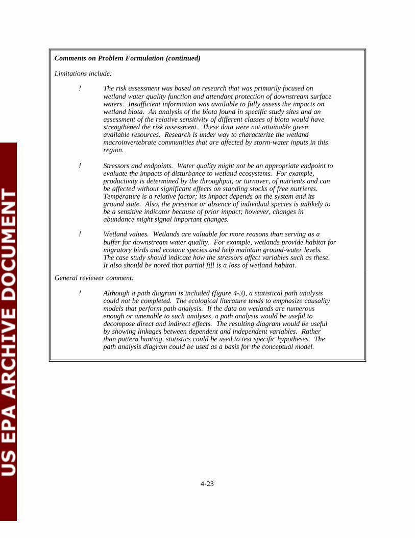
Comments on Problem Formulation (continued)
Limitations include:
! The risk assessment was based on research that was primarily focused on wetland water quality function and attendant protection of downstream surface waters. Insufficient information was available to fully assess the impacts on wetland biota. An analysis of the biota found in specific study sites and an assessment of the relative sensitivity of different classes of biota would have strengthened the risk assessment. These data were not attainable given available resources. Research is under way to characterize the wetland macroinvertebrate communities that are affected by storm-water inputs in this region.
! Stressors and endpoints. Water quality might not be an appropriate endpoint to evaluate the impacts of disturbance to wetland ecosystems. For example, productivity is determined by the throughput, or turnover, of nutrients and can be affected without significant effects on standing stocks of free nutrients. Temperature is a relative factor; its impact depends on the system and its ground state. Also, the presence or absence of individual species is unlikely to be a sensitive indicator because of prior impact; however, changes in abundance might signal important changes.
! Wetland values. Wetlands are valuable for more reasons than serving as a buffer for downstream water quality. For example, wetlands provide habitat for migratory birds and ecotone species and help maintain ground-water levels. The case study should indicate how the stressors affect variables such as these. It also should be noted that partial fill is a loss of wetland habitat.
General reviewer comment:
! Although a path diagram is included (figure 4-3), a statistical path analysis could not be completed. The ecological literature tends to emphasize causality models that perform path analysis. If the data on wetlands are numerous enough or amenable to such analyses, a path analysis would be useful to decompose direct and indirect effects. The resulting diagram would be useful by showing linkages between dependent and independent variables. Rather than pattern hunting, statistics could be used to test specific hypotheses. The path analysis diagram could be used as a basis for the conceptual model.
4-23
4.3.3. Analysis: Characterization of Exposure
4.3.3.1. Stressor Characterization
Among the study sites, dredging impacts ranged from minimal (no change in water depth class; e.g., Minnehaha site 39, type 5) to an increase in three depth units for site 36. In the latter case, a type 2 wetland was dredged to form a type 5 wetland pond. Impoundment in the absence of dredging was relatively rare, occurring at only two study sites, and resulted in a step change of only one unit in the scale of relative water depth (1-5).
Wetland fill area varied from 0.01 ha (Comma, site 38) to 2.0 ha (Colonial Pond, site 1), with percent wetland area filled ranging from less than 1 percent (Comma) to 71 percent (Colonial Pond). The greatest potential erosion impacts occurred at Centerville (site 31), with a ratio of 120 for construction zone to wetland area, indicating a high potential loading of sediment per unit surface area of wetland.
New storm-water inputs were common in urbanizing regions as the area of impervious surface increased and point-source storm sewers were built to divert storm water into wetlands. The potentially greatest storm-water impacts occurred at JP-26W (site 29), with an increase in the ratio of urban plus residential area to wetland area of 56. In two cases, ground water also was pumped into wetlands as a means to de-water adjacent construction sites. These inputs were temporary and sporadic and could not be quantified easily.
4.3.3.2. Ecosystem Characterization
Wetlands ranged in size from 0.01 ha to over 112 ha, and watersheds varied from 3.3 ha to 8,864 ha. Predominant land use in each watershed was classified as agricultural, urban or residential, or undeveloped or open space. Overall land use ranged from 0 to 92 percent agricultural, from 0 to 45 percent forested, from 0 to 48 percent urban, from 0 to 49 percent residential, from 1 to 58 percent water (lake plus marsh), from 0 to 70 percent construction area, and from 0 to 9 percent orchard in any given watershed. Average watershed slope varied from 1.4 percent for the Coon Creek watershed within the Anoka Sand Plain (site 23) to 13.2 percent for JP-25 (site 40) in the hilly terrain of Eagan. Soil erodability varied from an average K-factor of 0.16 (Coon Creek watershed, site 23) to an average K-factor of 0.33 in JP-68 (site 28) within Eagan.
Only a small proportion of the sites modified by physical or hydrological disturbance had buffers of undisturbed vegetation left surrounding the wetland. Typically, construction extended to the edge of or directly into the wetland. Only six wetlands had vegetated buffer zones left between the impact and the sampling point; these buffers ranged in width from 3 to 8 meters.
Effects of physical or hydrologic stressors will be moderated or exacerbated by climate, particularly the amount and temporal distribution of precipitation. Climate in the TCMA is continental, with mild, humid summers and relatively long, severe winters. Most rain comes in frontal storms or warm-weather convective storms, with May and June typically the wettest months and February the driest (Brown, 1984). Normal annual precipitation is 68.6 cm, including the water content of 111.8 cm average winter snowfall. Annual precipitation varied greatly during the study. In the drought year of 1989, annual precipitation was only 59.2 cm, while heavy summer rains brought the 1990 total to 83.9 cm (U.S. Weather Service, 1991).
Impacts on wetlands from physical and hydrologic disturbance depend in part on initial hydrologic and vegetation conditions at each site. Investigators classified the range of wetland types in the study area using the definitions in Circular 39 (Shaw and Fredine, 1956). Predominant vegetation in the wet meadows included reed canary grass (Phalaris arundinacea), smartweeds (Polygonum spp.), and stinging nettle (Urtica dioica). Cattail (Typha spp.) dominated both shallow and deep marshes, with sizable inclusions of softstem bulrush (Scirpus validus), giant reed grass (Phragmites australis), and
4-24

arrowhead (Sagittaria latifolia). Various pondweeds (Potamogeton spp.), coontail (Ceratophyllum demerusum), and water milfoil (Myriophyllum spp.) were common among submersed vegetation, with lotus (Nelumbo lutea), yellow water lily (Nuphar variegata), white water lily (Nymphaea odorata), and duckweed (Lemna spp.) floating on the surface of wetland ponds. Invasions of purple loosestrife (Lythrum salicaria) were found in scattered areas. Typical shrubs in type 6 wetlands included red osier dogwood (Cornus stolonifera), speckled alder (Alnus rugosa), and numerous willows (Salix spp.). Of the species noted, seven were rated as moderately tolerant to turbidity and pollution by Kadlec and Wentz (1974), while only one species (Potamogeton natans) was rated as relatively intolerant. Typha spp. and Phragmites australis, common at many of the sites, are considered to be invasive species that often appear in disturbed areas.
4.3.3.3. Exposure Analysis
Frequency of impacts due to physical or hydrologic disturbance to wetlands in the TCMA was quantified by two related survey approaches. First, information on all impending physical or hydrologic disturbances to wetlands in the TCMA for the period of fall 1988 to fall 1990 was requested from area resource managers (see above). Second, all individual and nationwide U.S. ACOE 404 permits requiring predischarge notification received in 1988 and 1989 by the St. Paul District U.S. ACOE Office were reviewed for information on factors related to permit success (Taylor et al., 1992).
The frequency of disturbance regimes at sampling stations was tabulated by Circular 39 wetland type (figure 4-4). Most sites received multiple impacts. Almost all study sites (79 percent) were potentially affected by sedimentation from construction activity immediately surrounding the wetland or from physical modifications to existing wetlands. Nearly two-thirds of the study sites were partially filled or affected by storm-water or pumped ground-water inputs. Added water inputs were most common for wetland pond or deep marsh systems, while water level changes due to dredging or impoundment were most common for shallow marsh or wet meadow systems.
A total of 114 fill permits were reviewed, of which 86 (75 percent) were approved. Investigators identified 30 (35 percent) approved permits for which additional disturbances at the wetland site were anticipated, either as part of a construction project, mitigation action, or water level manipulation for waterfowl management. Eighteen (60 percent) of the additional disturbances
4-25


involved dredging open water areas, five (17 percent) involved new storm-water inputs, four (13 percent) involved dredging channels, three (10 percent) involved impoundment but no dredging, and three (10 percent) involved wetland drainage (two cases of temporary drainage).
Most of the wetland sites identified in this study received more than one physical or hydrologic disturbance, and many sites obviously had been affected by past alterations. Without a longer term record, however, it was not possible to determine the frequency of disturbance to wetlands in the TCMA over time. The season during which the physical activity creating physical or hydrologic disturbances ends is probably the most critical aspect of timing that will affect wetland recovery. At 34 (72 percent) of the 47 mid-wetland stations monitored, the physical activity producing the wetland disturbance ended outside of the growing season, i.e., in the fall, over the winter, or during snowmelt.
It is clear that physical or hydrologic disturbances affect some wetlands in the TCMA more heavily than others. However, there is no evidence that fill permit success is significantly associated with wetland type, adjacency to large wetland complexes, adjacency to calcareous fens (which have special protection status in the state of Minnesota), or state-protected status (types 3, 4, and 5 wetlands; Taylor et al., 1992). Permits to fill wetlands immediately surrounded by industrial or commercial land or by open land (on the suburban fringe) are significantly more likely to be approved than those for wetlands immediately surrounded by residential, mixed residential, or agricultural land use (Taylor et al., 1992). Storm water-related disturbances to wetlands are prevalent in the Eagan area (northern Dakota County), which has a relatively steep topography and a rapid rate of growth through residential development (figure 4-1).
An exact percentage of the area of wetland resources in the TCMA affected annually by physical or hydrologic disturbance cannot be easily quantified until automated data are available from NWI map digitization. Wetlands of 10 to 500 acres in size were partially catalogued in 1967 by MN DNR for fish and wildlife management (MN DNR, 1967). According to their records, approximately 745 type 2, 3, 4, or 5 wetlands were found in the TCMA. No quantitative inventory of smaller wetlands is available. If 86 wetlands are partially filled in a 2-year period, 30 of which experience physical or hydrologic disturbances, this represents an incidence of approximately 11.5 percent of wetlands affected by partial fill and 4 percent of wetlands affected by additional physical or hydrologic disturbance over a 2-year period. This obviously is an overestimate, however, because many of the wetlands affected by fill and related disturbances are much smaller than 10 acres in size, and this fraction of the wetland resource has not been well quantified in the TCMA.
Total wetland losses in Minnesota resulting from 404 permits (individual, general, and nationwide) equaled approximately 1,196 acres out of a total of 5.02 million acres, or 0.024 percent per year in 1988-1989. During the same period, Minnesota also saw a gain due to mitigation activities of 1,135 acres, for a net loss rate of 0.0013 percent per year (MPCA, 1990). In comparison, wetland losses due to drainage in a 10-county area during 1974-1980 were estimated at 0.02 percent per year for wetland ponds, 0.6 percent per year for deep marshes, and 2.3 percent per year for shallow marshes (MPCA, 1990). Loss of specific wetland types as the result of conversions to other wetland types has not been quantified for this region of the country. Nationwide, 0.1 percent and 1.3 percent of forested palustrine wetland area (swamps) have been lost by conversion to nonvegetated wetlands (ponds) and marshes, respectively, while 0.2 percent of marshes has been lost to conversion to ponds (Dahl et al., 1991).
4.3.3.4. Exposure Profile
The most commonly recorded physical or hydrologic disturbances to wetlands in the TCMA are, in order of frequency, sedimentation from excessive erosion, wetland fill, deepening by dredging or impoundment, and storm-water impacts. Up to 11.5 percent of wetlands in the TCMA were permitted for partial or complete filling over a 2-year period, with up to 4 percent of all wetlands affected by additional physical or hydrologic disturbances. Wetlands on the suburban fringe or those surrounded by industrial or commercial land uses are most likely to be filled. Storm-water inputs are probably most common in areas of rapid residential growth and relatively steep topography, but the use of wetlands for
4-27
storm-water management is not well documented on a regional basis. Most disturbances to wetlands occur or terminate during a period outside of the growing season, thus maximizing potential recovery time.
Comments on Characterization of Exposure
Strengths of the case study include:
! Spatial and temporal variability in exposures is described.
! The causes of uncertainty in exposure estimates are documented.
Limitations include:
! A complete exposure profile for the TCMA wetlands would require that the potential resources affected be better quantified in terms of wetland number, area, and type. In addition, a more complete sample of physical and hydrologic disturbance frequency and intensity, particularly for partially regulated or nonregulated disturbances (drainage, impoundment, dredging, storm-water or pumped ground-water inputs) is needed.
! A more complete exposure profile also would include site-specific information on particular wetland populations and communities exposed to physical and hydrologic disturbance, as determined by the overlap of their temporal and spatial distributions. Some of this information will be available from an ongoing study of effects of storm-water and nonpoint-source pollution on wetland macroinvertebrate communities in the TCMA.
4.3.4. Analysis: Characterization of Ecological Effects
4.3.4.1. Evaluation of Relevant Effects Data
Investigators judged the relevance of the impacts of disturbance on wetland water quality on the basis of (1) the statistical significance of effects and (2) the potential ecological significance of effects. The statistical significance of changes in water quality was tested both as a verification of cause-and-effect relationships and as a means of comparing water quality values against a reference (predisturbance) condition. Comparisons against reference conditions are appropriate when water quality varies regionally as a function of landscape or climatic conditions or when there is a high level of uncertainty associated with the magnitude of critical effect levels. For example, reference conditions by ecoregion have been used in deriving regional lake water quality standards for the State of Minnesota (Heiskary and Wilson, 1990). Water quality criteria provide critical effect levels, but these often are derived based on tests of nonwetland species and under testing conditions (high dissolved oxygen, low dissolved organic carbon, circumneutral pH) that are atypical of wetlands (Hagley and Taylor, 1991).
The realism inherent in field-scale manipulations or observations is accompanied by spatial (geographic) variability among study sites as well as temporal (climatic) variability between pre- and postdisturbance periods. Analyses of predisturbance wetland water quality identified wetland type, hydrologic class, contact with sediment (pore water vs. surface water), season (snowmelt vs. growing season), and surrounding land use as factors with significant contributions to variability in wetland water quality variables (Detenbeck et al., 1991a). Thus, paired before-and-after comparisons were used to factor out spatial variability among sites. Predisturbance conditions at each site served as a reference against which peak- or postdisturbance conditions were compared using a parametric multivariate analysis of variance (MANOVA). A nonparametric Kruskal-Wallis test was used when data could not be
4-28

normalized with log transformations (Sokal and Rohlf, 1981). MANOVAs were used in place of paired t-tests to reduce the probability of Type II errors, which increases as the number of tests performed increases. Repeated analysis of variance measures by variable type would be an ideal test to use here to determine time to recovery because these tests would correct for possible carry-over effects (serial correlation), but the number of observations available without missing data for all of the time periods of interest was very low (n=8-9).
The disadvantage of a paired before-and-after comparison approach is that interannual climatic variability can bias changes between pre- and postdisturbance periods. Thus, only those water quality variables showing both (a) a significant change from predisturbance periods and (b) a significant difference in response among disturbance classes were considered to be affected by physical disturbances. Alternatively, one could employ paired before-and-after comparisons with sites distributed along a disturbance gradient, somewhat analogous to an analysis of covariance approach. This approach regresses the change in mid-wetland water quality at each site against indices of disturbance intensity. Thus the y-intercept represents the expected change in water quality due to interannual climate variability alone, while the slope of the regression represents the response to increasing disturbance intensity. A multiple regression approach can be used to factor out the effect of multiple disturbances as long as colinearity (correlation among dependent variables) is not a problem.
Evaluation of levels of water quality variables (or changes in water quality) associated with potential ecological effects was based on water quality criteria values (total lead, ammonia, total phosphorus, nitrate, dissolved oxygen, temperature, conductivity, and turbidity) or on critical effect levels derived from the literature (color, turbidity, total phosphorus, and conductivity). Individual states are still in the process of modifying narrative and numeric surface water quality criteria for application to wetlands. According to guidance provided to individual states by the EPA Office of Wetlands Protection, initial narrative and numeric water quality standards for wetlands should be developed or modified using existing information as much as possible, with a longer-term goal of developing biocriteria for wetlands (U.S. EPA, 1991). Relevant water quality standards associated with designated (protected) uses for surface waters in the State of Minnesota are listed in table 4-4.
4-29

Table 4-4. State of Minnesota Water Quality Criteria for Surface Waters by Designated Use (U.S. EPA, 1988c)
Water Quality State of MN a or Other Numeric Water Quality Criteria Variable Units
Total phosphorus :g P/L Recreation.b 40 :g P/L for North Central Hardwood Forest ecoregion
NO3 + NO2 mg N/L Consumption. >10 mg N/L
NH4 mg N/L For NH3-N. Fisheries & Recreation. A: >0.016 mg/L; B: >0.04 mg/L
Surficial dissolved mg/L Fisheries & Recreation. 2A: $7 mg/L at all times. 2B, 2C: $5 mg/L at all oxygen times
Surficial water temperature
deg C Fisheries & Recreation. A: no material increase, 30°C max. 8B, C: no increase in monthly avg. of max. daily temp. >1.7°C in lakes, 35°C max.
Total extractable lead :g/L 4-day average. >1.3, 3.2, or 7.7 :g/L at 50, 100, 200 mg CaCO3/L hardness
Specific conductivity :mhos/cm Agr. & Wildlife. A: >700 mg/L TDSc
Turbidity NTUd Fisheries & Recreation. A: >10; B, C: >25
aDepending on attainable use (Fisheries & Recreation or Agriculture & Wildlife). Class A = associated with salmonid fisheries, Class B = supporting cool- and warm-water sport or commercial fisheries and associated aquatic community, Class C = supporting indigenous fish and associated aquatic community.
bBased on attainable lake trophic state for North Central Hardwood Forest ecoregion. cApprox. 1,094 :mhos/cm. TDS = total dissolved solids. dNTU = nephelometric turbidity units.
Table 4-5. Water Quality Values Associated With Mean Light Requirements of 21.4 Percent Incident Radiation for Submerged Aquatic Vegetation in Northern Lakes (Chambers and Kalff, 1985)
Wetland Type
Depth Range, cm Kd, m-1
Secchi Depth, meters
Turbidity, FTUa
Color, PCU
Total P, : g/L
III 15-60 2.57 0.64 11.4 583 107
IV 60-120 1.28 1.29 5.2 268 N/Ab
V 120-240 0.64 2.58 2.2 113 N/Ab
aFTU = formazin turbidity units.bSecchi depths outside of range of observations used in deriving equation.
4-30

.
Changes in color, turbidity (suspended solids), and trophic state (total phosphorus [TP]) can be evaluated based on their effects on wetland transparency and on the potential for successful growth of submerged macrophyte communities. Relatively few data have been published on light requirements for submerged aquatic plants. Data have been compiled for sea grasses (Dennison et al., 1993) and for submerged macrophytes in the littoral zone of northern lakes (Chambers and Kalff, 1985). Chambers and Kalff report an average minimal light requirement for freshwater angiosperms in Canadian lakes corresponding to 21.4 ± 2.4 percent of surface light levels. Corresponding color, turbidity, and chlorophyll a levels, which would reduce light at the bottom of a type III, type IV, or type V wetland to 21.4 percent of surface illumination, can be calculated (table 4-5).
Calculations were based on the following relationships:
Equation 4-1 (Wetzel, 1975):
Kd = extinction coefficient = ln (I0/Iz) × 1/z = ln (1/0.214) × 1/zmax,m
where I0 = incident radiation, Iz = radiation at depth z
Secchi depth = 1.65/Kd (Dennison et al., 1993)
Equation 4-2 (Brezonik, 1978):
1/S.D. = 0.106 + 0.128 (turbidity, nephelometric turbidity units [NTU]) + 0.0025 (color, platinum cobalt units [PCU])
Equation 4-3:
log10(Secchi depth, cm) = 2.07 ! 0.13 log10(total P, :g/L)
(Derived from data for colored lakes with average depth <2.4 m, in Beaver and Crisman, 1991.)
Minnesota's standard of 40 :g P/L for TP in lakes within the North Central Hardwood Forest is lower than the estimated requirement of 107 :g P/L to maintain sensitive submerged aquatic macrophyte communities in type III wetlands. The lower standard is ecoregion based and is designed to minimize the frequency of nuisance algal blooms.
During predisturbance conditions, mean specific conductivity values for surface water (440 :mhos/cm) and ground water (610 :mhos/cm) were near the upper end of the range associated with freshwater vegetation in the glaciated prairie region. Stewart and Kantrud (1971) list a range of <40-500 :mhos/cm for normal climatic conditions and a range of <40-700 :mhos/cm for extreme (drought) conditions. Thus, 700 :mhos/cm was considered a threshold value for specific conductivity for these wetlands.
Investigators had to apply dissolved oxygen criteria derived for other surface waters to study area wetlands because of a lack of better literature values. These criteria, however, were probably overprotective since wetlands in the study area typically contain no fish or fish species extremely tolerant of low dissolved oxygen (e.g., common carp [Cyprinus carpio], fathead minnow [Pimephales promelas], and brook stickleback [Culaea inconstans]). However, investigators believed that the average level and diurnal fluctuations in both dissolved oxygen and temperature could be critical in determining acceptable spawning habitat or refugia for amphibians.
4-31

4.3.4.2. Ecosystem Response Analyses
Investigators could not use MANOVA to test categorical effects with the full complement of study sites because data matrices were complete for a subset of sites; the power of these tests was more limited than for regression analyses. However, MANOVAs did demonstrate a significant fivefold increase in soluble reactive phosphorus (SRP) and a threefold increase in dissolved phosphorus (DP) at the peak of storm-sewer disturbance activities (after storm sewers were connected and during watershed construction activity; table 4-6). Threefold increases in SRP and DP were still evident in storm water-impacted sites at 6 to 12 months and at 12 to 24 months following peak disturbance. Nitrate levels were strongly elevated, fortyfold in dredged or impounded sites and eightfold in storm water-impacted sites during the peak of disturbance activity, but no significant (categorical) increases were observed during subsequent time intervals (table 4-6). All increases were significant at a probability level (") of 0.05, some at a probability level of 0.001.
To assess further the long-term impacts of construction and residential development surrounding wetlands in urbanizing areas, nonparametric Kruskal-Wallis tests were used to compare different categories of wetlands. Wetlands in nondeveloping watersheds experienced declines in dissolved nitrogen between predisturbance and recovery periods, while those wetlands in developing watersheds experienced no change or a slight increase in dissolved nitrogen. Construction activity in the watershed was associated with increased ln (total suspended solids [TSS]) within wetlands in the second year following disturbance (Detenbeck et al., 1992).
Comparison of water quality changes among wetlands with or without vegetated buffers in watersheds with or without construction activity showed significant effects (p<0.05) only with respect to the initial impact period at the peak or immediately following disturbance. Wetlands without vegetated buffers in watersheds with construction activity had greater SRP levels than either wetlands associated with construction activity but surrounded by vegetated buffers or wetlands in watersheds without new construction activity. There was no significant difference between peak or predisturbance SRP for wetlands in watersheds without new construction activity and those surrounded by vegetated buffers. Nitrate levels followed the same pattern as SRP levels (Detenbeck et al., 1992).
DP was least in wetlands with no construction activity in the surrounding watershed but did not show significant differences between buffered and nonbuffered wetlands. Dissolved nitrogen and water color were greater in nonbuffered wetlands than in watersheds without construction activity. Longer-term effects of buffers were not detected for growing season averages of water quality variables in the first year following disturbance (p>0.05).
4-32

Table 4-6. Summary of Results of MANOVAs Testing for Significant Difference in Water Quality Change Among Disturbance Classes for Each of Four Time Periods
Average ln Ratio (post/pre)a
(geometric mean) (back-transformed 95% CI)
Time Variable Periodb N Depth Change Wetland Fill Storm Water
)ln soluble reactive phosphorus
)ln dissolved phosphorus
)ln nitrate
)ln dissolved phosphorus
)ln soluble reactive phosphorus
)ln dissolved phosphorus
)ln dissolved phosphorus
1 19 -0.038 -0.090 1.65c
(5.2) (1.7 - 16)
1 19 -0.37 -0.081 1.21d
(3.4) (1.6 - 7.2)
1 19 3.68d -0.30 2.02d
(39.6) (7.5)(10.4 - 151) (2.9 - 19.7)
3 16e 0.24 -0.32 1.15c
(3.2) (1.3 - 7.3)
4 14e 0.17 -0.44 1.09c
(3.0) (1.2 - 7.6)
4 14e 0.11 -0.48 1.15c
(3.2) (1.4 - 7.2)
4 21 0.16 -0.39 0.71c
(2.0) (1.1 - 4.8)
aDifferences in the change in water quality between disturbance classes were tested by Tukey's test to control for experimentwise error. Categories not significantly different from each other are indicated by a line. Only variables demonstrating a significant change in water quality and significant differences in response among disturbance regime categories are included here.
(Notes continued on next page)
4-33

b1 = Peak-disturbance vs. predisturbance.2 = 0-6 months postdisturbance vs. predisturbance.3 = 6-12 months postdisturbance vs. predisturbance.4 = 12-24 months postdisturbance vs. predisturbance.
cDifferent from zero: p<0.05.dDifferent from zero: p<0.01.eOnly data for which both dissolved and total constituents were available (surface water samples) were includedin the analysis.
4-34

4.3.4.3. Analyses Relating Measurement and Assessment Endpoints
The impact of physical or hydrologic disturbance on mid-wetland water quality depends on the ecological significance of the observed magnitude of change. In addition, potential impacts on biota of downstream surface waters must be considered. The impact of changes on water quality variables for which numeric water quality criteria exist or threshold values have been derived can be evaluated by assessing the incidence of criteria or threshold value exceedance.
4.3.4.4. Stressor-Response Profile
Investigators used stepwise multiple regression analysis to assess the effects of the intensity of physical or hydrologic disturbances on mid-wetland water quality. The change in water quality between pre- and postdisturbance time periods was the dependent variable. Although numerous statistically significant relationships were found, this case study reports on a subset focusing on water quality variables for which threshold values were derived or criteria were available (table 4-7). Equations were reported in greater detail by Detenbeck and colleagues in earlier reports (1991a, 1992).
Storm-water inputs, construction, dredging or impoundment, wetland fill, and increases in watershed area or area of urban or residential land use had a significant effect on mid-wetland water quality. Construction, particularly within the buffer zone surrounding wetlands, was correlated with increased concentrations of suspended solids, total lead, and nitrate in wetlands during the first year following disturbance. Increased urbanization relative to wetland area tended to increase total nutrient levels and the fraction of nutrients associated with particulate matter. Particulate nitrogen and phosphorus tended to increase as the area of wetland fill increased. Storm-water inputs (quantified as an increase in impervious surface area) tended to decrease dissolved nutrient levels in wetlands, probably by decreasing the water retention time of the wetlands (Detenbeck et al., 1992; Brown, 1985). When predisturbance mid-wetland water quality data were compared among sites, wetlands in isolated basins had significantly higher nutrient, dissolved organic carbon, and color values than did wetlands with intermittent or continuous flow. In effect, connecting previously isolated wetlands with a storm-water sewer network can flush nutrients downstream. Deepening wetlands by impoundment or dredging tended to lessen some
4-35

Table 4-7. Equations Predicting Change in Mid-Wetland Water Qualitya as a Function of Disturbance Intensity (adapted from Detenbeck et al., 1991a, 1992)
Independent Independent Time Period Disturbanc Dependent Variableb Variableb
Comparison n Adj. r2 e Regime Variable X1 X2 Equation
Spring,ln (post/pre) 6 0.70 Storm water TP URB/WTLD WSHD/WTLD Y = -1.4 + 0.20 X1 - 0.07 X2
Spring,ln (post/pre) 6 0.91 Storm water Color CONSTRN/WTLD WSHD/WTLD Y = -1.3 + 0.09 X1 - 0.055 X2
Spring,ln (post/pre) 5 0.80 Storm water Total extr. Pb ln CONSTRN/WTLD Y = -1.8 + 0.46 X1
ln (during/pre) 88 0.82 Fill SRP TYPEDIFF FILL Y = -1.8 - 3.7 X1 + 4.3 X2
ln (during/pre) 7 0.54 Fill Color TYPEDIFF Y = -0.3 - 1.0 X1
ln (post/pre) 9 0.78 Depth SRP WSHD/WTLD FILL/WTLD Y = 1.7 + 0.007 X1 - 12 X2change
ln (post/pre) 6 0.90 Depth TP CONSTRN/WTLD WSHD/WTLD Y = -0.6 + 0.08 X1 + 0.022 X2change
Spring,ln (post/pre) 7 0.91 Depth Color TYPEDIFF WSHD/WTLD Y = 0.6 -3.1 X1 + 0.0045 X2
change
Spring,ln (post/pre) 7 0.42 Depth TSS WSHD/WTLD Y = -0.2 + 0.008 X1
change
ln (recov/pre) 15 0.47 All SRP RES/WTLD Y = -0.3 + 0.16 X1
ln (recov/pre) 12 0.61 All TP U+R/WSHD WSHD/WTLD Y = -0.2 + 6 X1 - 0.2 X2
aGrowing season average unless otherwise stated.bAreas in hectares: WTLD = wetland area; WSHD = watershed area; FILL = hectare fill area; TYPEDIFF = change in wetland depth (1-5);RES = residential area in watershed; U+R = urban + residential area in watershed.
4-36

changes in mid-wetland water quality, probably by increasing retention time and sedimentation efficiency.
Regression analyses also were used to determine the effect of disturbance intensity on recovery during the second year following disturbance. By that time, neither area of wetland filled nor percentage of wetland filled nor change in wetland type (water depth) had a discernible effect on mid-wetland water quality. However, changes in watershed land use relative to either watershed area or wetland area produced long-term effects on wetland water quality. Increases in urban or residential land use were associated with increases in dissolved nutrients (SRP, DP, N, and DOC) and TP and decreases in surface dissolved oxygen. An increase in the percentage of watershed developed (percentage urban and residential) was associated with a long-term increase in TP and decrease in surface water temperature. Construction activity in the watershed was correlated with decreased SRP and increased levels of suspended solids. As relative watershed area (and flushing rate) increased, dissolved N and P and TP tended to decrease, offsetting some of the increase due to accelerated nutrient loading.
Comments on Characterization of Ecological Effects
Strengths of the case study include:
! A statistical analysis of ecosystem responses was conducted, allowing estimates of response along a gradient of disturbance as well as categorical response. Uncertainties due to Type I errors can be quantified.
Limitations include:
! Expected impacts due to water quality changes were derived in part from criteria developed for surface waters other than wetlands.
! Habitat impacts were not measured directly.
! Only static endpoints were used; ecological processes were not measured.
General reviewer comments:
! EPA is developing biocriteria to address ecological effects, but these criteria are not yet available for wetlands.
! Indices of abiotic ecological quality, e.g., habitat destruction, should be linked to biota.
4.3.5. Risk Characterization
4.3.5.1. Risk Estimation
Investigators did not detect significant changes in mid-wetland specific conductivity, temperature, dissolved oxygen, or ammonium levels between pre- and postdisturbance periods, nor were any significant differences in response noted among disturbance categories by MANOVA. Peak-, postdisturbance-, or recovery-period-specific conductivity levels exceeded the threshold value of 700 :mhos.cm-1 in three cases, and temperature levels exceeded the absolute criteria for Minnesota lakes (35°C) in one case (table 4-8).
4-37

Table 4-8. Mean and Range of Growing Season Mid-Wetland Water Quality Values Prior to and Following Disturbance
Water Quality Growing Season Growing Season Peak-Variable Units Predisturbance Mean (range) Disturbance Mean (range)a Postdisturbance Mean (range) Postdisturbance Mean (range)
Growing Season 1st Yr Growing Season 2nd Yr
Total :g P/L 593 (29-2,806) F 690 (110-1,712) 167 (25-766) 212 (25-904) phosphorus D 312 (42-2,426) 261 (36-2,733) 375 (46-1,639)
S 182 (32-511) 218 (23-996) 157 (40-559) M 132 (45-292) 159 (64-385) 272
NO3+NO2 mg N/L 0.43 (0.01-7.03) F 0.55 (0.03-1.41) 0.16 (0.01-0.90) 0.21 (0.01-0.99) D 0.19 (0.01-0.79) 0.13 (0.01-0.86) 0.07 (0.01-0.34) S 0.19 (0.01-1.25) 0.07 (0.01-0.31) 0.03 (0.01-0.06) M 0.09 (0.06-0.12) 0.17 (0.03-0.61) 0.01
NH4 mg N/L 0.32 (0.01-2.61) F 0.05 (0.01-0.13) 0.13 (0.01-1.93) 0.15 (0.01-0.98) D 0.11 (0.01-0.91) 0.14 (0.01-2.53) 0.17 (0.01-2.03) S 0.03 (0.01-0.05) 0.08 (0.01-0.60) 0.07 (0.01-0.15) M 0.38 (0.21-0.49) 0.92 (0.06-2.67) 0.05
Surficial mg/L 7.1 (1.2-15.4) F 9.1 (8.4-10.6) 9.0 (3.5-12.4) 7.9 (3.0-16.0) dissolved D 4.5 (0.6-8.8) 5.8 (0.6-14.6) 3.1 (0.6-7.5) oxygen S 9.5 (2.7-13.6) 7.6 (1.3-20) 7.4 (1.3-14.8)
M 6.8 (5.0-9.6) 4.9 (2.5-7.6) 12.0
Surficial ° C 16.6 (9.5-25.5) F 18.8 (14.5-24.0) 19.4 (8.0-29.5) 21.4 (7.0-34.0) water D 20.4 (14.0-29.3) 18.8 (8.0-28.0) 22.1 (12.0-29.0) temperature S 22.3 (16.2-36) 20.0 (11.0-29.0) 21.0 (12.0-33.0)
M 17.1 (10.8-21) 17.7 (13.0-25.0) 22.0
Total extractable lead :g/L 9 (surface) 34 (porewater)
Specific conductivity :mhos/cm 398 (107-928) F 133 (80-188) 300 (132-850) 283 (70-504) D 327 (164-759) 330 (153-688) 260 (162-404) S 239 (99-465) 216 (126-481) 206 (162-277) M 1120 (1,097-1,153) 758 (299-1,460) 283
Color PCU 150 (32-746) F 232 (34-601) 96 (40-226) 104 (38-260) D 140 (41-342) 150 (38-448) 131 (61-468) S 99 (19-343) 91 (26-305) 77 (44-135) M 48 (17-100) 82 (5-176) 170
Turbidity NTU 24 (2-98) F 282 (26-735) 27 (1-84) 15.2 (1-62) D 26 (3-127) 14 (1-279) 26 (3-128) S 34 (2-201) 19 (1-80) 12 (3-28) M 63 (15-133) 40 (3-123) 34
aF = partially filled, D = depth change (usually increase), S = storm-water or pumped ground-water inputs, M = multiple.
4-38
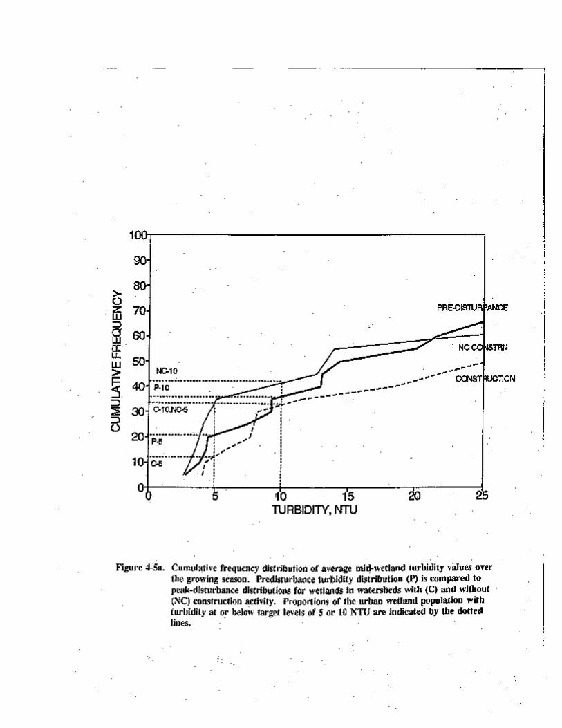


The change in surface water temperature (as evidenced by the upward shift in minimum, mean, and maximum values between pre- and postdisturbance conditions) was >1.7°C for most cases, but differences in temperature increase were not noted among disturbance classes. This level of temperature variability may be natural for shallow wetland systems that are less resistant to temperature than are lakes.
Surficial dissolved oxygen levels were occasionally below the lower limit criteria for Class B and C waters for both predisturbance conditions (7 percent) and postdisturbance conditions (23 percent; table 4-8). Under the range of pH values measured for similar wetlands in the metropolitan area (pH 6-8; Detenbeck et al., 1991a) and the temperature range observed for these wetlands (7-36°C), approximately 2 to 11 percent of total ammonia plus ammonium would be present in the toxic (un-ionized) form (Thurston et al., 1974). Levels of total ammonium in wetlands during the predisturbance period were high enough to exceed Minnesota's water quality criteria for Class B and C fisheries and recreation surface waters (0.04 mg NH3-N/L; U.S. EPA, 1988a) at approximately 60 percent of sites under the highest pH and temperature conditions observed. The proportion of sites at potential risk declined over the next 2 years to 5 to 15 percent following disturbance.
Mid-wetland nitrate levels increased significantly immediately following depth changes due to impoundment or dredging (39.6×) or immediately following storm-water inputs (7.5×). In no instance did nitrate levels exceed water quality criteria for drinking water standards; in general, nitrate levels were 1 to 3 orders of magnitude below the criteria of 10 mg N/L. However, if these wetlands are nitrogen-limited, a sevenfold to fortyfold increase in nitrate could be expected to stimulate productivity dramatically.
For water quality variables showing a significant categorical response to disturbance, the change in risk to wetland water quality or potential water quality function can be expressed as a frequency of criteria exceedance for pre- and postdisturbance populations. The majority of wetlands studied had predisturbance turbidity levels exceeding target levels for type III wetlands (64 percent >10 NTU) and type IV wetlands (21 percent >5 NTU; figure 4-5a). At the peak of disturbance, the frequency of sites exceeding target levels for type III wetlands decreased slightly for wetlands with no construction activity in the watershed (to 58 percent) and increased slightly for wetlands with construction activity in the watershed (to 66 percent; figure 4-5a). However, in the first year following disturbance, average turbidity levels exceeded target levels for type III wetlands for 37 percent of sites with no construction activity, and turbidity levels exceeded the target level of 10 NTU for 84 percent of sites exposed to construction activity (figure 4-5b).
4-41


Total extractable lead levels were quite high in the dry predisturbance period, possibly because of increased availability of lead following oxidation of lead sulfides or increased chelation by elevated dissolved organic carbon levels. The predisturbance average for surface water was 9 :g Pb/L, well above the criteria of 7.7 :g/L for chronic toxicity at a hardness level of 200 mg CaCO3/L. Maximum mid-wetland lead levels declined between the pre- and postdisturbance periods, possibly due to increased precipitation and a lowering of redox levels. However, the magnitude of the inter-annual decrease in total lead decreased as a function of construction activity in the period immediately following storm-water inputs (figure 4-6).
The level of construction activity in the watershed associated with exceedance of the water quality criteria for chronic toxicity was calculated as a function of initial lead levels. Figure 4-6 shows the level of the ln (construction/wetland area) ratio associated with exceedance of the criteria for chronic toxicity (3.2 :g/L at 100 mg/L CaCO3 hardness) corresponding to the 95th percentile, 75th percentile, and 50th percentile (median) values of predisturbance lead levels. Four of six sites had construction activity greater than that associated with criteria exceedance for the upper 5 percent of predisturbance values, three sites had levels associated with criteria exceedance for the upper 25 percent of predisturbance values, and two cases had construction activity (ln ratio >2.9, ratio >18.2) higher than that associated with exceedance for sites in the upper half of the predisturbance distribution. Similar predictions can be derived for other initial lead distributions. Predictions are based on mean response (ln [post/pre] Pb); the actual response is expected to fall within the 95 percent confidence interval for the regression.
Mid-wetland TP levels exceeded target levels derived to protect clarity of type III wetlands (107 ppb P) and criteria for Minnesota lakes in the North Central Hardwood Forest ecoregion (40 ppb P) in the majority of cases for predisturbance, peak-disturbance, postdisturbance, and recovery periods (70 to 80 percent >107 ppb P, 94 to 100 percent >40 ppb P). Based on results of regression analyses, potential increases in TP for storm water-impacted sites related to urbanization were offset by increased flushing rate related to increased watershed/wetland area ratios.
Investigators used regression equations for mid-wetland TP to predict stressor levels associated with criteria or threshold value exceedance for different percentiles of the population of predisturbance wetland conditions (figures 4-7a-d). For wetlands associated with the lower 50 percent of predisturbance TP levels, springtime TP levels were expected to exceed target levels of 40 ppb P and 107 ppb P for wetlands experiencing depth changes of <2.4 or <1.4 units, respectively (figure 4-7a). For the upper 75th percentile of sites, a target level of 40 ppb P could be achieved in cases of little or no construction activity (construction/wetland area <5) and a net decrease in watershed/wetland area (-13 to -30; figure 4-7b). The lower 50th percentile of cases were expected to remain below the target level of 107 ppb P only for cases of limited construction activity (ratio of 0 to 8) and no change or a decrease in watershed/wetland area (figure 4-7c). For wetlands affected by storm water, the lowest 50th percentile could achieve the target level of 40 ppb P following disturbance for increases in the urbanization ratio of up to 8, but only if relative watershed size (and flushing rate) was increased proportionately (figure 4-7d).
Color levels were elevated during predisturbance (drought) conditions corresponding to high dissolved organic carbon levels (Detenbeck et al., 1991a). However, only 2 percent of sites had color levels exceeding the target of 583 PCU for type III wetlands, approximately 20 percent
4-47


of wetlands had color >268 (target for type IV wetlands), and 50 percent had color >113 PCU (target for type V wetlands) during the predisturbance period. Color alone probably is not limiting submerged macrophyte production in these systems. Maximum color levels for wetlands in fill and storm-water disturbance categories decreased following disturbance activities but increased between peak-disturbance and recovery periods for dredge or impoundment cases in response to increased watershed/wetland area ratios. Isopleth plots showing combinations of depth change and change in watershed/wetland for which target color levels could be achieved show that color levels are relatively insensitive to changing watershed/wetland area ratios and that the lowest target level for color is achievable for the lower 50th percentile given a small increase in depth (figure 4-8).
4.3.5.2. Uncertainty
Sources of uncertainty in this risk assessment include both qualitative errors (e.g., errors in assumptions) and quantitative errors (e.g., measurement or prediction errors). Table 4-9 lists the main sources of uncertainty in each phase of the risk assessment, along with an estimate of the magnitude of uncertainties.
Information gaps related to quantifying the total wetland resource in TCMA and the true frequencies of physical or hydrologic disturbances to wetlands contributed to overestimation and underestimation, respectively, of the true incidence of anthropogenic disturbance. Information gaps on direct habitat loss or conversion rates and lack of (tested) water quality criteria specific to wetlands limited the investigators' ability to create a balanced assessment of impacts to the full wetland ecosystem as compared with impacts to downstream surface waters.
Sources of uncertainty in the empirical field study on impacts and recovery included the interaction of effects of climatic variability between pre- and postdisturbance periods with effects of anthropogenic physical or hydrologic disturbance. By using the paired comparison regression approach, investigators were able to factor out potential additive effects of climatic differences between years but were not necessarily able to factor out interactive (e.g., multiplicative) effects. The design of the study would have been improved by including information from paired comparisons of undisturbed reference sites. Finally, the risk assessment could be improved by a separate field validation of regression predictions based on a separate set of study sites.
4-49

Table 4-9. Uncertainties Affecting Measurement of Risk to Urban Wetland Water Quality Status and Water Quality Improvement Function Related to Physical or Hydrologic Disturbance
Phase of Risk Assessment Level/Measure of Uncertainty
Characterization of Exposure
Total area, number of wetlands in metropolitan area
Incidence of physical or hydrologic disturbances to metropolitan area wetlands over time
Intensity of physical disturbances to wetlands in metropolitan region
Conversion factors for wetlands in metropolitan region
Unknown certainty; no quantitative updated inventory available
Unknown, especially for unregulated activities
Range, distribution of measured values
Unknown extrapolation error from nationwide trend analysis
Characterization of Ecological Effects
Selection of threshold values or pertinent water quality criteria
Estimate of relative risk due to habitat loss vs. water quality degradation
Measurement extrapolations
Precision/accuracy of water quality measurements
Probability of Type I error in identifying significant changes in water quality
Stressor-response analysis
Unknown certainty: (a) surface water quality criteria derived for clearwater lakes and streams, not wetlands; (b) water quality threshold values to protect transparency based on relationships derived for colored lakes and macrophyte depth distributions for relatively clearwater lakes
Direct effects of habitat loss or conversion on threatened or endangered species not measured
Temperature and dissolved oxygen min./max. values not recorded
Loadings to downstream surface waters not directly measured
Relative error generally <10 percent
p #0.05
Type I error #0.05; uncertainty of predicted response indicated by regression r2 values, 95 percent confidence intervals
4-50

4.3.5.3. Risk Description: Summary and Interpretation of Ecological Significance
Table 4-10 compares the risk to urban wetland water quality and water quality improvement function from physical or hydrologic disturbance to potential loss or conversions of wetland habitat. While neither dredging nor impoundment activity (water-depth change) caused many significant long-term changes in mid-wetland water quality, these activities probably had the greatest effect on wetland habitat. Wetland habitat is permanently removed by wetland fill activity and severely modified by dredging operations. Although emergent vegetation began to recover at disturbed wetland sites within 1 year following disturbance, the recovery of submerged vegetation appeared to be delayed by more than 2 years, especially where organic substrates had been removed (Detenbeck et al., 1992). Similarly, storm-water additions create a significant long-term shift in hydrologic regime, which may affect vegetation succession patterns and spawning habitat for amphibians.
4-51

Table 4-10. Summary of Risk to Urban Wetland Water Quality Status and Water Quality Improvement Function Assessed Against Loss or Conversion of Wetland Habitat
Percentage of Percentage of Metropolitan Nature/Probability of Direct Metropolitan Area Wetlands Predicted Metropolitan Wetland Area Habitat Loss Through to Exceed Water Quality Criteria or Potential for Water
Activity Wetlands Affected a Affected Destruction or Conversion Threshold Values (%) Quality Recovery
Fill 5.75%/yr 0.024% Estimated mitigation of 94.9% 94-100% >40 :g P/L, Recovery of all water of losses statewide 70-80% >107 :g P/L quality parameters in <1 yr
(historical impacts)
Dredge/impoundment 4.8%/yr 100% type conversion for 94-100% >40 :g P/L, Incr. NO3 <1 yr dredged/impounded sites 70-80% >107 :g P/L Nationwide conversion rates: (historical impacts) 0.1% type 7 to 5 1.3% type 7 to 3, 4 0.2% type 3, 4 to 5
Storm water 1.0%/yr (new); cum. Permanent change in 94-100% >40 :g P/L, Incr. Pb, NO3 <1 yr; freq. approaching hydrologic regime 70-80% >107 :g P/L potential release of Pb 100% in some areas (historical impacts) during drought
Incr. turbidity >1 yr 33% of storm water-impacted sites had Incr. SRP, DP >2 yrs construction activity high enough to produce spring Pb levels >3.2 :g/L on average
Construction 4.5%/yr Type conversion due to 94-100% >40 :g P/L, Incr. TSS > 2 years siltation at rate of 3%/yr for 70-80% >107 :g P/L sites adjacent to construction (historical impacts) activity
84% >10 NTU in first year following construction
Drainage 0.3%/yr 100% habitat loss; historical losses reversing at rate # 0.08%/yr of current area through restoration
aBased on frequency of fill impacts and percentage of filled wetlands experiencing additional impacts.
4-52

4-53
Although the immediate effects of wetland fill on surface water quality are limited, the long-termcumulative effect of the loss or conversion of wetland area must be considered in determining risk toaquatic resources in this region. Earlier studies demonstrated a relationship between the extent ofwetlands and low total lead or high color in downstream lakes, and between proximal wetlands andlowered trophic status in downstream lakes, or lowered suspended solids, fecal coliform, nitrate, and flow-weighted NH4 or TP in streams of the TCMA region (Johnston et al., 1990; Detenbeck et al., 1991b,1993).
Given the high level of total extractable lead in wetlands during the predisturbance period, anyincrease in lead would be considered detrimental to both wetland biota and biota of downstream surfacewaters. However, in the absence of disturbance activity, average total lead levels were predicted todecrease by 84 percent due to interannual climatic variation alone to levels just above detection limits. There is a high degree of uncertainty as to the actual impact of total extractable lead in wetland systemsfor two reasons. Surface water quality criteria were derived under standard testing conditions of lowdissolved oxygen content, which may affect the availability of lead to biota. Second, much of the leadtrapped in wetlands is associated with particulate matter, so that sediment concentrations and the potentialfor bioaccumulation need to be assessed (Stockdale, 1991).
Long-term categorical impacts on mid-wetland water quality were observed in response toconstruction activity and storm-water inputs (increased total and volatile suspended solids) or in responseto residential development in the watershed (increased dissolved nitrogen). The proportion of wetlandswith turbidity greater than identified thresholds for protection of submerged macrophyte communitiesincreased over the first year following construction activity. The ecological significance of increaseddissolved nitrogen in these systems is unknown at this point but could be very important if this change isan indicator of disruption of nitrogen cycling (Detenbeck et al., 1992).
Changes in land use (residential and urban development) and watershed area relative to wetlandarea were associated with statistically significant impacts on nutrients and water color in the first andsecond years following disturbance. However, it is clear that the trophic status of these wetlands is highdue to prior loading. For fully or partially impounded wetlands, cumulative effects of wetlandeutrophication may occur over time as loadings continue, but longer term studies are needed to assessthese effects (Kadlec, 1985). Increased loadings of SRP or TP to wetlands converted from isolatedpotholes to components of storm water networks that experience intermittent or continuous flow probablycreate greater risks to downstream surface waters than to the wetlands themselves. The inverserelationship between watershed/wetland area and mid-wetland phosphorus concentrations for storm-water wetlands suggests that increased nutrient loads are being flushed downstream (Detenbeck et al.,1992). Given the high proportion of eutrophic and phosphorus-limited lakes in the TCMA, any additionalinputs of phosphorus to downstream lakes are likely to be detrimental to these systems (MetropolitanCouncil, 1981).
Best management practices, such as the use of vegetated buffers, were only partially protectiveof mid-wetland water quality. Storm water represents a point-source input and is not filtered by vegetatedzones surrounding wetlands. Vegetated buffers were associated with lower SRP and nitrate in wetlandswith construction activity in the surrounding watershed, but this moderating effect was only temporary.
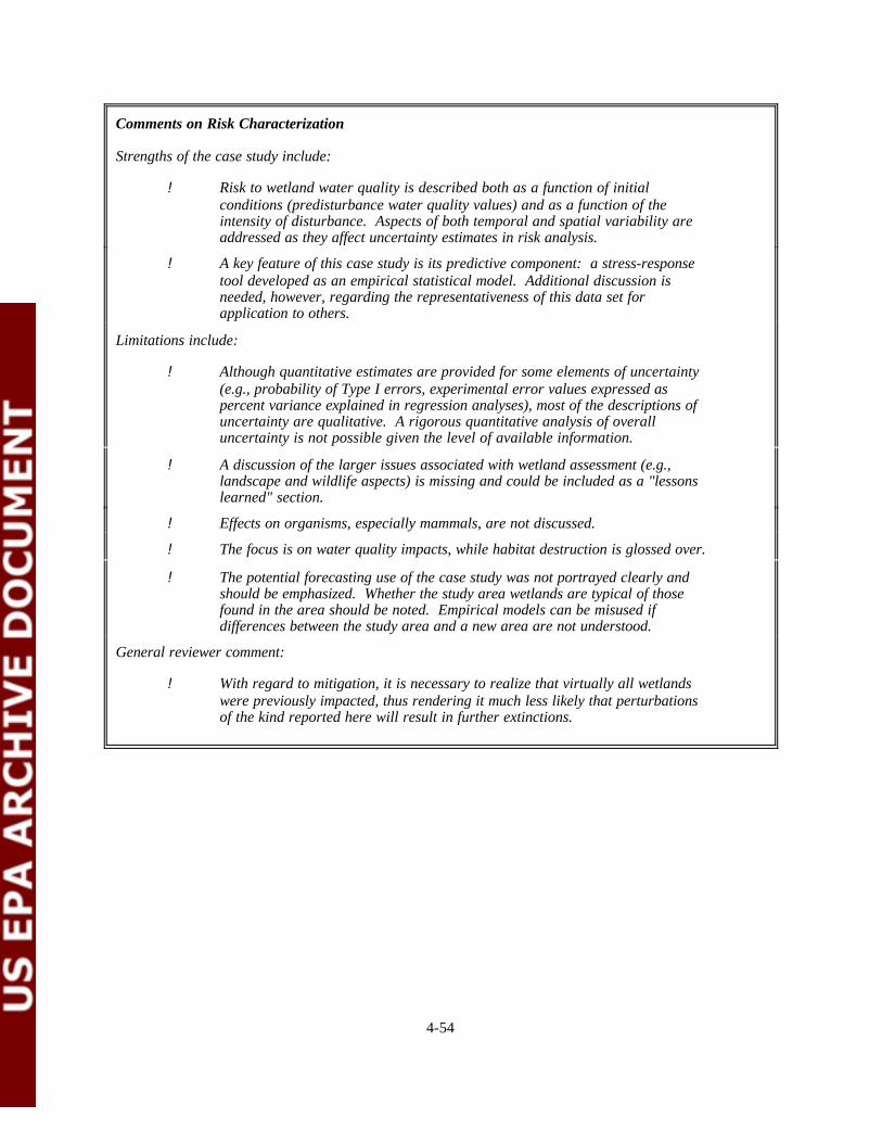
4-54
Comments on Risk Characterization
Strengths of the case study include:
! Risk to wetland water quality is described both as a function of initialconditions (predisturbance water quality values) and as a function of theintensity of disturbance. Aspects of both temporal and spatial variability areaddressed as they affect uncertainty estimates in risk analysis.
! A key feature of this case study is its predictive component: a stress-responsetool developed as an empirical statistical model. Additional discussion isneeded, however, regarding the representativeness of this data set forapplication to others.
Limitations include:
! Although quantitative estimates are provided for some elements of uncertainty(e.g., probability of Type I errors, experimental error values expressed aspercent variance explained in regression analyses), most of the descriptions ofuncertainty are qualitative. A rigorous quantitative analysis of overalluncertainty is not possible given the level of available information.
! A discussion of the larger issues associated with wetland assessment (e.g.,landscape and wildlife aspects) is missing and could be included as a "lessonslearned" section.
! Effects on organisms, especially mammals, are not discussed.
! The focus is on water quality impacts, while habitat destruction is glossed over.
! The potential forecasting use of the case study was not portrayed clearly andshould be emphasized. Whether the study area wetlands are typical of thosefound in the area should be noted. Empirical models can be misused ifdifferences between the study area and a new area are not understood.
General reviewer comment:
! With regard to mitigation, it is necessary to realize that virtually all wetlandswere previously impacted, thus rendering it much less likely that perturbationsof the kind reported here will result in further extinctions.

4.4. REFERENCES
Adamus, P. (1989) Wetlands and water quality: EPA's research and monitoring implementation plan for the years 1989-1994. Environmental Research Laboratory, Office of Research and Development, U.S. Environmental Protection Agency, Corvallis, OR.
Anderson, J.P.; Craig, W.J. (1984) Growing energy crops on Minnesota's wetlands: the land use perspective. Center for Urban and Regional Affairs, University of Minnesota, Minneapolis, MN.
Ayers, M.A.; Brown, R.G.; Oberts, G.L. (1985) Runoff and chemical loading in small watersheds in the Twin Cities metropolitan area, Minnesota. U.S. Geological Survey, Water Resources Investigation Report 85-4122, St. Paul, MN.
Beaver, J.R.; Crisman, T.L. (1991) Importance of latitude and organic color on phytoplankton productivity in Florida lakes. Can. J. Fish. Aquat. Sci. 48(7):1145-1150.
Brezonik, P.L. (1978) Effect of organic color and turbidity on Secchi disc transparency. J. Fish. Res. Board Can. 35:1410-1416.
Brown, R.G. (1984) Atmospheric deposition of selected chemicals and their effect on nonpointsource pollution in the Twin Cities metropolitan area, Minnesota. U.S. Geological Survey, Water Resources Investigation Report 83-4195, St. Paul, MN.
Brown, R.G. (1985) Effects of wetlands on quality of runoff entering lakes in the Twin Cities metropolitan area, Minnesota. U.S. Geological Survey, Water Resources Investigation Report 85-4170, St. Paul, MN.
Chambers, P.A.; Kalff, J. (1985) Depth distribution and biomass of submersed aquatic macrophyte communities in relation to Secchi depth. Can. J. Fish. Aquat. Sci. 42:701-709.
Cowardin, L.M.; Carter, V.; Golet, F.C.; LaRoe, E.T. (1979) Classification of wetlands and deepwater habitats of the United States. Biological Services Program, U.S. Fish and Wildlife Service. FWS/OBS-79-31.
Dahl, T.E.; Johnson, C.E. (1991) Status and trends of wetlands in the conterminous United States, mid-1970's to mid-1980's. U.S. Department of the Interior, Fish and Wildlife Service, Washington, DC.
Dennison, W.C.; Orth, R.J.; Moore, K.A.; Stevenson, J.C.; Carter, V.; Kollar, S.; Bergstrom, P.W.; Batiuk, R.A. (1993) Assessing water quality with submersed aquatic vegetation. Bioscience 43(2):86-94.
Detenbeck, N.E.; Johnston, C.A.; Taylor, D.L.; Lima, A.; Hagley, C.A.; Bamford, S. (1991a) Effects of disturbance on water quality functions of wetlands: final report to the U.S. EPA. Environmental Research Laboratory-Duluth. Natural Resources Research Institute, University of Minnesota and AScI Corporation, Duluth, MN.
Detenbeck, N.E.; Johnston, C.A.; Niemi, G.J. (1991b) Use of a geographic information system to assess the effect of wetlands on lake water quality in the Minneapolis/St. Paul metropolitan area. In: Proc. of the MN Lake Management Conference. Brainerd, MN, October 7-9, 1990, pp. 81-85.
Detenbeck, N.E.; Taylor, D.L.; Lima, A. (1992) Assessing recovery of freshwater wetland water quality from disturbance. Final report to U.S. EPA, Environmental Research Laboratory, Duluth, MN.
4-55
Detenbeck, N.E.; Johnston, C.A.; Niemi, G.J. (1993) Wetland effects on lake water quality in the Minneapolis/St. Paul metropolitan area. Landscape Ecol. 8:39-61.
Eggers, S.D.; Reed, D.M. (1987) Wetland plants and plant communities of Minnesota and Wisconsin. U.S. Army Corps of Engineers, St. Paul District.
Galinato, M. (1985) Seed germination studies of dominant wetland species of the Delta Marsh. M.S. thesis, Dept. of Botany, Iowa State University, Ames, IA.
Gosselink, J.G.; Lee, L.C. (1989) Cumulative impact assessment in bottomland hardwood forests. Wetlands, vol. 9 (special issue), 174 pp.
Hagley, C.A.; Taylor, D.L. (1991) An approach for evaluating numeric water quality criteria for wetlands protection. Report to the U.S. EPA, Environmental Research Laboratory, Duluth, MN.
Heiskary, S.A.; Wilson, C.B. (1990) Regional patterns in lake water quality in Minnesota. Lake Line 10(6):26-30.
Johnston, C.A.; Detenbeck, N.E.; Niemi, G.J. (1990) The cumulative effect of wetlands on stream water quality and quantity: a landscape approach. Biogeochemistry 10:105-141.
Kadlec, R.H. (1985) Aging phenomena in wastewater wetlands. In: Godfrey, P.J.; Kaynor, E.R.; Pelczarski, S.; Benforado, J., eds. Ecological considerations in wetlands treatment of municipal wastewaters. Chapter 23. New York, NY: Van Nostrand Reinhold Company.
Kadlec, J.A.; Wentz, W.A. (1974) State-of-the-art survey and evaluation of marsh plant establishment techniques: induced and natural. Volume I: Report of research. U.S. Army Corps of Engineers Waterways Experiment Station. Vicksburg, MS.
Leibowitz, S.; Preston, E.M.; Arnaut, L.Y.; Detenbeck, N.E.; Hagley, C.A.; Kentula, M.E.; Olson, R.K.; Sanville, W.D.; Sumner, R.R. (1992) Wetland research plan FY92-96: an integrated risk-based approach. U.S. EPA, Environmental Research Laboratory, Corvallis, OR. EPA/600/R-92/060.
Leslie, M.; Clark, E.H. II. (1990) Perspectives on wetlands loss and alterations. In: Bingham, G.; Clark, E.H. II; Haygood, L.V.; Leslie, M., eds. Issues in wetlands protection: background papers prepared for the National Wetlands Policy Forum. Chapter 1. Washington, DC: The Conservation Foundation.
Metropolitan Council. (1981) A 1980 study of the water quality of 60 lakes in the Twin Cities metropolitan area. Publication 01-81-047. Metropolitan Council, St. Paul, MN.
Minnesota Department of Natural Resources (MN DNR). (1967) Metropolitan lake inventory. Bulletin 45. Minnesota Dept. of Natural Resources, St. Paul, MN.
Minnesota Department of Natural Resources (MN DNR). (1984) Minnesota official list of endangered, threatened, and special concern plants and animals. Minnesota Dept. of Natural Resources, St. Paul, MN.
Minnesota Pollution Control Agency (MPCA). (1990) Minnesota water quality: water years 1988-1989. 1990 Report to Congress. Minnesota Pollution Control Agency, St. Paul, MN.
Niering, W.A. (1985) The Audubon Society nature guides: wetlands. New York, NY: Alfred A. Knopf, Inc.
4-56

Omernik, J.M. (1986) Ecoregions of the conterminous United States map (scale 1:7,500,000). U.S. Environmental Protection Agency, Environmental Research Laboratory, Corvallis, OR.
Osborne, L.L.; Wiley, M.J. (1988) Empirical relationships between land use/cover and stream water quality in an agricultural watershed. J. Environ. Mgmt. 26:9-27.
Owens, T.; Meyer, M. (1978) A wetlands survey of the Twin Cities 7-county metropolitan area-east half. IAFHE FSL Research Report 78-2. University of Minnesota, St. Paul, MN.
Rushton, B. (1991) Variation in field parameters in a native wetland used for storm water treatment. In: Rushton, B.; Cunningham, J.; Dye, C., eds. Statewide stormwater management workshop, October 2, 1991. Brooksville, FL: South Florida Water Management District, pp. 75-84.
Shaw, S.P.; Fredine, C.G. (1956) Wetlands of the United States. Circular 39. U.S. Dept. of the Interior, Fish and Wildlife Service. Washington, DC: U.S. Government Printing Office, 1971 (reissue).
Sokal, R.R.; Rohlf, F.J. (1981) Biometry: the principles and practice of statistics in biological research. 2nd ed. San Francisco, CA: W.H. Freeman and Company.
Stewart, R.E.; Kantrud, H.A. (1971) Classification of natural ponds and lakes in the glaciated prairie region. Resource Publication 92. U.S. Dept. of the Interior, Fish and Wildlife Service. 57 pp.
Stockdale, E.C. (1991) Freshwater wetlands, urban stormwater, and nonpoint source pollution control: a literature review and annotated bibliography. Washington State Department of Ecology.
Taylor, D.L.; Detenbeck, N.E.; Lima, A. (1992) Patterns of wetland disturbance in the Minneapolis-St. Paul metropolitan area: implications for policy makers. Unpublished manuscript.
Thurston, R.V.; Russo, R.C.; Emerson, K. (1974) Aqueous ammonia equilibrium calculations. Technical Report Number 74-1. Fisheries Bioassay Laboratory, Montana State University, Bozeman, MT. 18 pp.
Tiner, R.W., Jr. (1984) Wetlands of the United States: current status and recent trends. U.S. Dept. of the Interior, Fish and Wildlife Service, Washington, DC.
U.S. Army Corps of Engineers. (1992) Public Notice, 14 February 1992. U.S. Army Corps of Engineers, St. Paul District.
U.S. Environmental Protection Agency. (1986) Hazard evaluation division standard evaluation procedure: ecological risk assessment. Office of Pesticide Programs, Washington, DC. EPA-540/9-85-001.
U.S. Environmental Protection Agency. (1988a) Nitrogen-ammonia/nitrate/nitrite: water quality standards criteria summaries: a compilation of state/federal criteria. EPA 440/5-88/029.
U.S. Environmental Protection Agency. (1988b) State water quality standards summaries. Office of Water Regulations and Standards, Washington, DC. EPA 440/5-88/031.
U.S. Environmental Protection Agency. (1991) National guidance: water quality standards for wetlands. Office of Water Regulations and Standards, Office of Wetlands Protection, Washington, DC. EPA 440/S-90-011.
4-57

U.S. Environmental Protection Agency. (1992) Framework for ecological risk assessment. Risk Assessment Forum, Washington, DC. EPA/630/R-92/001.
U.S. Weather Service. (1991) Minneapolis-St. Paul Airport, MN. Personal communication.
Walker, W. (1987) Phosphorus removal by urban runoff detention basins. Lake and Reservoir Management 3:314-326.
Werth, J.; Meyer, M.; Brooks, K. (1977) A wetlands survey of the Twin Cities 7-county metropolitan area-west half. IAFHE RSL Research Report 77-10. University of Minnesota, St. Paul, MN.
Wetzel, R.G. (1975) Limnology. Philadelphia, PA: W.B. Saunders Company.
4-58

SECTION FIVE
ECOLOGICAL RISK ASSESSMENT CASE STUDY:
THE ROLE OF MONITORING IN ECOLOGICAL RISK ASSESSMENT: AN EMAP EXAMPLE

AUTHORS AND REVIEWERS
AUTHORS
John H. GentileEnvironmental Research Laboratory - NarragansettU.S. Environmental Protection AgencyNarragansett, RI
K. John ScottScience Applications International CorporationNarragansett, RI
John F. PaulEnvironmental Research Laboratory - NarragansettU.S. Environmental Protection AgencyNarragansett, RI
Rick A. LinthurstAtmospheric Research and Exposure Assessment LaboratoryU.S. Environmental Protection AgencyResearch Triangle Park, NC
REVIEWERS
Robert J. Huggett (Lead Reviewer)Virginia Institute of Marine ScienceThe College of William and MaryGloucester Point, VA
Gregory R. BiddingerExxon Biomedical Sciences, Inc.East Millstone, NJ
Joel S. BrownUniversity of Illinois at ChicagoChicago, IL
Richard E. Purdy Environmental Laboratory 3-M Company St. Paul, MN
Frieda B. Taub School of Fisheries University of Washington Seattle, WA
Richard Weigert Department of Zoology University of Georgia Athens, GA
5-2

CONTENTS
ABSTRACT . . . . . . . . . . . . . . . . . . . . . . . . . . . . . . . . . . . . . . . . . . . . . . . . . . . . . . . . . . . . . . . . 5-6
5.1. RISK ASSESSMENT APPROACH . . . . . . . . . . . . . . . . . . . . . . . . . . . . . . . . . . . . . . . . . . . . 5-8
5.2. STATUTORY AND REGULATORY BACKGROUND . . . . . . . . . . . . . . . . . . . . . . . . . . . . . . . . 5-8
5.3. CASE STUDY DESCRIPTION . . . . . . . . . . . . . . . . . . . . . . . . . . . . . . . . . . . . . . . . . . . . . . . 5-10
5.3.1. Problem Formulation . . . . . . . . . . . . . . . . . . . . . . . . . . . . . . . . . . . . . . . . . . . . . . . . 5-12
5.3.1.1. Background . . . . . . . . . . . . . . . . . . . . . . . . . . . . . . . . . . . . . . . . . . . . . . . 5-125.3.1.2. Site Description . . . . . . . . . . . . . . . . . . . . . . . . . . . . . . . . . . . . . . . . . . . . 5-125.3.1.3. Ecosystem Classification . . . . . . . . . . . . . . . . . . . . . . . . . . . . . . . . . . . . . . 5-135.3.1.4. Sampling Design . . . . . . . . . . . . . . . . . . . . . . . . . . . . . . . . . . . . . . . . . . . . 5-135.3.1.5. Ecological Indicators . . . . . . . . . . . . . . . . . . . . . . . . . . . . . . . . . . . . . . . . . 5-14
5.3.2. Conceptual Model Development . . . . . . . . . . . . . . . . . . . . . . . . . . . . . . . . . . . . . . . . . 5-17
5.3.2.1. Ecological Effects . . . . . . . . . . . . . . . . . . . . . . . . . . . . . . . . . . . . . . . . . . . 5-175.3.2.2. Exposure . . . . . . . . . . . . . . . . . . . . . . . . . . . . . . . . . . . . . . . . . . . . . . . . . 5-215.3.2.3. Exposure-Response Associations . . . . . . . . . . . . . . . . . . . . . . . . . . . . . . . . 5-245.3.2.4. Estuarine Class Conceptual Models . . . . . . . . . . . . . . . . . . . . . . . . . . . . . . . 5-265.3.2.5. Problem Formulation Summary . . . . . . . . . . . . . . . . . . . . . . . . . . . . . . . . . 5-28
5.3.3. EMAP and Regional Risk Assessments . . . . . . . . . . . . . . . . . . . . . . . . . . . . . . . . . . . . 5-30
5.3.3.1. Regional Risk Assessment: Problem Formulation . . . . . . . . . . . . . . . . . . . . . 5-315.3.3.2. Regional Risk Assessment: Analysis Phase . . . . . . . . . . . . . . . . . . . . . . . . . 5-315.3.3.3. Regional Risk Assessment: Risk Characterization . . . . . . . . . . . . . . . . . . . . . 5-32
5.4. REFERENCES . . . . . . . . . . . . . . . . . . . . . . . . . . . . . . . . . . . . . . . . . . . . . . . . . . . . . . . . . . 5-37
5-3

LIST OF FIGURES
Figure 5-1. Structure of assessment for EMAP Virginian Province . . . . . . . . . . . . . . . . . . . . . . . . . 5-9
Figure 5-2. EMAP Virginian Province base stations for 1990-1991. . . . . . . . . . . . . . . . . . . . . . . . . 5-11
Figure 5-3. Contribution of EMAP data to problem formulation . . . . . . . . . . . . . . . . . . . . . . . . . . . 5-18
Figure 5-4. Summary of Virginian Province response and exposure indicator values for the entireprovince, large tidal rivers, large estuaries, and small estuarine systemsfor 1990 and 1991 data, individually and combined . . . . . . . . . . . . . . . . . . . . . . . . . . . 5-22
Figure 5-5. EMAP estuaries indicator relationships, 1990 and 1991 base stations . . . . . . . . . . . . . . . 5-29
LIST OF TABLES
Table 5-1. Summary of EMAP Response and Exposure Indicator Data for 1990-1991 . . . . . . . . . . 5-19
Table 5-2. Indicator Associations: The Percent Area of Degraded Benthos Co-occurring With Low Dissolved Oxygen and Sediment Toxicity for EMAP Base Stationsfor 1990-1991. . . . . . . . . . . . . . . . . . . . . . . . . . . . . . . . . . . . . . . . . . . . . . . . . . . . . 5-25
COMMENT BOX
Comments on Problem Formulation, Conceptual ModelDevelopment, and Regional Risk Assessments . . . . . . . . . . . . . . . . . . . . . . . . . . . . . . . . . . . . . . . . . 5-33
5-4

7 LIST OF ACRONYMS
EMAP Environmental Monitoring and Assessment Program
EPA Environmental Protection Agency
ER-M Effects Range-Median
GIS geographic information system
HEP Harbor Estuary Program
NEP National Estuary Program
NOAA National Oceanic and Atmospheric Administration
NPDES National Pollution Discharge Elimination System
NRC National Research Council
NS&T National Status and Trends Program
ORD Office of Research and Development
OTA Office of Technology Assessment
R-EMAP Regional EMAP
5-5

ABSTRACT
Using data collected from the Environmental Monitoring and Assessment Program's (EMAP's) Near Coastal program in the Virginian Biogeographic Province during July through September 1990-1991, this paper describes the role and specific contributions of monitoring data in the ecological risk assessment process. This case study suggests that EMAP monitoring data can:
# contribute to the problem formulation phase of an ecological risk assessment;
# characterize areal and spatial extent of ecological resources;
# identify regional resources potentially at risk (e.g., degraded benthos); and
# provide initial information on the role of exposure and habitat characteristics.
EMAP data were collected using a systematic probability-based sampling design that facilitates detection of spatially distributed patterns but does not estimate intra-annual variability or short-term episodic events. The EMAP information was then used to develop a conceptual model that described the areal extent of ecological resources at risk, their spatial distribution, and associated exposure and habitat information. The assessment endpoint was benthic community integrity. Resource condition, measured using a province-wide benthic index, was operationally defined in terms of one or more anthropogenic stressors. Currently, resource condition does not discriminate anthropogenic from natural physical stress.
In this case study, large estuaries exhibited the lowest areal extent of degraded benthos, 16±7 percent; low dissolved oxygen was the exposure indicator most closely associated with degradation. In small estuarine systems, 24±10 percent of the area exhibited degraded benthic condition, nearly half (48 percent) of which was associated with sediment toxicity. For large tidal rivers, 41±24 percent of the sampled area was degraded, and 45 percent of this degradation co-occurred with low dissolved oxygen. Co-occurrence of degradation and low dissolved oxygen was confined to the mouths of the Potomac and Rappahannock Rivers. Although these associations imply neither causality nor direct anthropogenic stress, they could, along with other evidence, be used to direct further study. In this regard, on a province basis more than half of the area of degraded benthos was not associated with any of the exposure indicators discussed.
Data on spatial distribution indicated that degradation of benthic resources occurred mainly in the upper Chesapeake Bay, the oligo-mesohaline portions of the five tidal river systems (e.g., Hudson-Raritan), and the associated small bays. These bays are areas of intense demographic pressure and extensive urban development.
Although useful in identifying regional areas of concern, EMAP province-scale data are not sufficient for conducting a complete risk assessment at the regional scale. Where local monitoring data are too heterogeneous (relative to spatial, temporal, and ecological scales and methodologies) to be usable in regional ecological risk assessments, investigators may need to acquire additional data through:
# an appropriately scaled monitoring program employing a random sampling design, such as the Regional EMAP [R-EMAP] program in EPA Region II;
# selection of the appropriate response, exposure, and habitat indicators to characterize the spatial extent of ecological problems and associated exposures; and
# incorporation of extant data (e.g., National Oceanic and Atmospheric Administration's [NOAA's] National Status and Trends [NS&T] Program, National Estuary Program [NEP], states, etc.).
5-6

Monitoring data alone cannot establish the causal relationships necessary to develop a complete analysis of ecological risk. Therefore, ecological risk assessments should include laboratory exposure-response information (e.g., ecotoxicity), effects of multiple stressors, and measures of contaminant bioavailability to provide evidence for postulating potential causes of risk to the region or to specific watersheds. Risks to specific watersheds can be examined initially by using geographic information system (GIS) and landscape methods that describe the spatial relationships and distribution of response, exposure, and habitat indicators (stressor-specific, whenever possible). This information can then be overlaid with landscape information on anthropogenic stressors and hydrologic features (e.g., transport and fate) in the surrounding watershed. Establishing causal relationships between sources and effects provides the basis for instituting appropriate control strategies. Ongoing local compliance (e.g., National Pollution Discharge Elimination System [NPDES], states, municipalities) and watershed assessment (e.g., R-EMAP, EMAP, NS&T, NEP) monitoring programs can evaluate the effectiveness of the control strategy.
5-7

5.1. RISK ASSESSMENT APPROACH
The U.S. Environmental Protection Agency's (EPA's) implementation of a risk-based assessment, monitoring, and decision-making strategy requires the integration of the Office of Research and Development's (ORD's) ecological risk assessment framework (U.S. EPA, 1992); research, monitoring, and assessment programs under ORD's Environmental Monitoring and Assessment Program (EMAP); and ORD's ecological risk assessment research programs. Successfully implementing a risk-based approach for decision making for adoption throughout EPA requires the integration of these three programs. The framework and process for conducting ecological risk assessment must not be separated from monitoring programs responsible for data acquisition and verification nor from research programs responsible for developing the needed methods and models. The combination of these programs provides the template for all ecological risk research, irrespective of specific programmatic applications, while ensuring that EPA can respond directly to the full spectrum of ecological risk assessment needs.
This case study illustrates the roles and contributions of EMAP's Near Coastal Program to the ecological risk assessment process as described by EPA's Framework for Ecological Risk Assessment. The case study also examines the use of monitoring data to identify potential problems for estuarine resources and the potential use of biogeographic province-scale information in regional assessments. Since EMAP and other monitoring programs typically are not designed to generate all the information required for a complete ecological risk assessment, this paper focuses specifically on the use of monitoring data (e.g., EMAP Virginian Biogeographic Province data from 1990 to 1991) in the problem formulation stage of the risk assessment process (figure 5-1). The areal extent and spatial patterns of ecological resources for the Virginian Province identify specific regional areas potentially at risk. The case study uses the Hudson-Raritan estuary as an example to illustrate the types of information needed for a complete ecological risk assessment.
5.2. STATUTORY AND REGULATORY BACKGROUND
The EPA, U.S. Congress, and private environmental organizations have long recognized the need to improve our ability to document the condition of our environment and specifically our ecological resources (National Research Council [NRC], 1990). Federal, state, and local agencies; waste dischargers; and researchers all conduct marine environmental monitoring. Five federal agencies conduct environmental quality monitoring activities in the coastal ocean. Each agency's programs focus on different spatial scales, ranging from effluent discharges from individual sources (e.g., EPA's National Pollutant Discharge and Elimination System [NPDES] Program) to measuring far-field, long-term effects of discharges from multiple sources (e.g., the National Oceanic and Atmospheric Administration's [NOAA's] National Status and Trends [NS&T] program, EPA's National Estuary Program [NEP]). However, these programs do not, either individually or taken together, constitute a comprehensive national status and trends monitoring program focused on contributing information for identifying the potential risks to coastal environmental resources (NRC, 1990). Congressional hearings on the Monitoring Improvement Act in 1984 (U.S. House of Representatives, 1984) concluded that, despite considerable expenditures on monitoring, federal agencies could assess neither the status of ecological resources nor the overall progress toward legally mandated goals of mitigating or preventing adverse ecological effects. In 1988, the EPA Science Advisory Board (U.S. EPA, 1988), affirming the existence of major gaps in environmental data and recognizing the broad base of support for better environmental monitoring, recommended that EPA initiate a program to monitor ecological status and trends of the nation's ecological resources. EMAP is EPA's response to these recommendations. This case study illustrates EMAP's contribution to the risk-based assessment framework that is the cornerstone of EPA's decision-making process.
5.3. CASE STUDY DESCRIPTION
This case study describes the role and contribution of monitoring data in the ecological risk assessment process. The EMAP response, exposure, and habitat indicator data presented in this case
5-8


study were collected from the estuarine waters of the Virginian Biogeographic Province, which extends from Cape Cod, Massachusetts, to Cape Henry, Virginia, at the mouth of the Chesapeake Bay (figure 5-2).
Information from response, exposure, and habitat indicators constitutes the data acquisition component of ORD's Framework for Ecological Risk Assessment and contributes directly to the problem formulation stage of the risk assessment process. The monitoring data specifically contribute to the development of a conceptual model that delineates the spatial, temporal, and ecological boundaries of the problem; the specific ecosystems and ecological components potentially at risk; and the potential exposure pathways and co-occurrence with ecosystem attributes/resources of concern.
This case study analyzed data collected during 1990-1991 by determining the cumulative percent area (i.e., cumulative distribution function) for each ecological response and exposure indicator for the entire province and its component resource classes (large estuaries, small estuarine systems, and large tidal rivers). Because the EMAP sampling design is based upon a 4-year sampling cycle, the areal estimates based on 2 years of data reported in this case study for the response and exposure indicators must be viewed as examples of how the data can be used and should not be construed as the most complete or accurate reflection of the power of the EMAP sampling design. Since EMAP uses a probability-based design, the results from 2 years of sampling are likely representative of the remaining 2 years. However, the additional data will improve the estimates of central tendency, decrease uncertainty, and increase the power to detect change.
Analyses examined the associations between response and exposure indicators to explore the potential reasons for the observed changes in ecological condition. The areal extent of resource change that co-occurred with the exposure indicators was determined for the province as a whole and for each resource class. Information on exposure-response associations focused attention on specific regional areas, such as the Delaware Bay and the Hudson-Raritan estuary. For these areas, a full ecological risk assessment—a reiteration of problem formulation, the analysis of causal relationships, and the characterization of risks—can be conducted if the data warrant. Although these types of analyses are straightforward, their interpretation deserves discussion.
A typical assumption implicit in interpreting results such as these is that changes in resource status (e.g., degraded or subnominal condition) result from anthropogenic stress. One must view such interpretations with caution since these data are not designed to provide definitive information on causality or to separate anthropogenic from natural stressors. Rather they provide a "weight of evidence" approach, suggesting the direction for additional data acquisition and research. These data also are the basis for developing testable hypotheses to explain observations regarding the status of ecological resources. For example, low dissolved oxygen and physical alterations of habitats may not have anthropogenic origin in certain situations; therefore, they should not be associated with degradation, as defined by EMAP. For this reason, EMAP primarily seeks to determine the status of ecological resources. Although a useful and important part of the program, understanding the reasons for changes in status is secondary.
Although not explicitly part of this case study, a regional scale risk assessment could use both historical data (e.g., NEP, states, EPA Regions, academia) and new data (e.g., Regional-EMAP, EMAP) to characterize the magnitude and extent of the problem at the regional scale. In addition, changes in ecological resources can be coupled to specific stressors. Using geographic information system (GIS) and landscape methods, these stressors can be linked to potential sources associated with land-based activities. The overall effectiveness of control strategies applied to point and nonpoint sources could then be evaluated by both compliance (e.g., NPDES, states, dischargers) and long-term monitoring programs (e.g., R-EMAP, EMAP, states). This case study illustrates the application of a risk-based assessment and monitoring strategy that provides direct and indirect evidence for inferring causal associations between the observed ecological effects and specific stressors, thus enabling the manager to plan and evaluate remedial control strategy options.
5-10

5.3.1. Problem Formulation
5.3.1.1. Background
Problem formulation, the initial phase of the ecological risk assessment process, consists of the following components: stressor and ecological effects characterization, identification of ecosystems potentially at risk, selection of assessment and measurement endpoints, and development of a conceptual model (U.S. EPA, 1992). The conceptual model synthesizes the information in each of these components to describe the potential stressors and exposure pathways; their co-occurrence, direct and indirect links with specific ecosystems and assessment endpoints of concern; the spatial, temporal, and ecological boundaries of the risk assessment; and inferences as to potential causal associations between stressors and ecological effects. In this case study, the conceptual model describes (1) the areal extent of degraded benthic resources, (2) the areal extent of exposure to specific categories of stressors, (3) the relationship between the areal extent of degraded benthic resources and exposure to categories of stressors, (4) the relative importance of different stressors in each estuarine ecosystem, and (5) specific regional estuarine systems with degraded benthic resources that could become the subject of detailed regional risk assessments. The following sections describe the EMAP indicators and analyze and interpret data for 1990 and 1991 to provide information for the conceptual model.
5.3.1.2. Site Description
The data were collected from the estuarine waters of the Virginian Biogeographic Province, which extends from Cape Cod, Massachusetts, to Cape Henry, Virginia, at the mouth of the Chesapeake Bay. Covering approximately 23,573 km2, the province includes several large estuarine systems (e.g., Chesapeake Bay, Delaware Bay, and Long Island Sound) as well as a substantial number of small estuarine systems and large tidal rivers (Holland, 1990). Both the Labrador Current and the Gulf Stream affect the Virginian Province, which has a continental/subtropical climate. Estuarine resources vary widely in size, shape, and ecological characteristics. Many estuaries, like Chesapeake Bay, are large, continuously distributed resources that consist of expansive regions with a broad variety of habitat types. Other estuaries consist of relatively discrete resources composed predominantly of one habitat type. For sampling design purposes, the estuarine waters of the Virginian Province were classified into three categories: large estuarine systems, large tidal rivers, and small estuarine systems.
5.3.1.3. Ecosystem Classification
Large estuarine systems are defined as systems having surface areas greater than 260 km2 and aspect ratios (length/average width) less than 20. Application of these criteria to the Virginian Province resulted in the identification of 12 large estuarine systems with a total surface area of 16,096 km2, or 70 percent of the province's estuarine area. Large tidal rivers were defined as systems having surface areas greater than 260 km2 and aspect ratios greater than 20. These criteria resulted in the identification of five large tidal rivers—Hudson, Potomac, James, Delaware, and Rappahannock Rivers—with a total surface area of 2,840 km2, or 13 percent of the total province area. Small estuarine systems were defined as systems having surface areas less than 260 km2 but greater than or equal to 2.6 km2. Application of these criteria to the Virginian Province resulted in the identification of 137 small estuarine systems with a total surface area of 4,279 km2, or 17 percent of the province.
The classification process categorized estuaries into classes (strata) for which a common sampling design can be used. The process also ensured that selected components of estuarine resources were sampled sufficiently in different systems. Further, the classification process facilitated the synthesis and integration of data into assessments for evaluating the effectiveness of management actions (Holland, 1990).
5-12

5.3.1.4. Sampling Design
The EMAP sampling design provides unbiased estimates of the status and trends in indicators of ecological condition with known confidence. There are four essential features of the EMAP sampling design as applied to estuaries: regionalization, classification, statistical sampling, and index period. A regionalization scheme partitions the estuarine and coastal resources of the United States into geographical areas with similar ecological properties. The classification scheme defines certain populations of interest (e.g., large estuaries, small estuarine systems, etc.) within large geographical areas that are functionally similar and can be sampled using a common approach. The value of the EMAP sampling design is that it is both systematic in areal coverage yet probabilistic relative to the sampling strategy (Overton et al., 1991). This design, therefore, can determine areal extent (with confidence intervals) and the spatial patterns of response, exposure, and habitat indicators irrespective of the characteristics of their statistical distributions. The statistical sampling provides for the determination of unbiased estimates of the status and trends of the estuarine ecological resource classes. When fully implemented, EMAP will base its status assessments on data collected over a 4-year baseline (Holland, 1990). This multiyear cycle was chosen to dampen the year-to-year variability resulting from natural phenomena such as extremely dry or wet years and hurricanes. A consistent, probability-based sampling design is employed within each EMAP resource group to facilitate future integrated assessments among EMAP resource groups (e.g., estuaries, surface waters, forests).
Fully characterizing natural seasonal variability or assessing status for all seasons is beyond the scope of EMAP. Because intra-annual variability is thought generally to exceed interannual variability, an index period (July to September) was chosen to represent that portion of the year when the measured parameters are expected to show the maximum response to pollutant stress (Connell and Miller, 1984; Sprague, 1985; Mayer et al., 1989), dissolved oxygen concentrations are lowest (Holland et al., 1987; U.S. EPA, 1984; Officer et al., 1984), fauna and flora are most abundant, and within-season variability is expected to be minimal. This sampling design may fail to detect short-term, episodic events. However, persistent unexplained degradation identified by EMAP would certainly stimulate additional research in the area of concern. This approach is consistent with EMAP’s goals of determining the long-term status and trends of ecological resources, with the status and trends then being used as the basis for intensive site-specific research to understand the reasons for the observed problems.
Sampling sites in the large estuarine class were selected using a randomly placed systematic grid. The distance between the systematically spaced sampling points on the grid was approximately 18 km. The grid is an extension of the systematic grid proposed for use by all EMAP resource groups (Overton et al., 1991). For the Virginian Province, 54 sample sites were identified for the large estuaries for 1990, and 48 sites in 1991. Sampling sites were limited to waters >2 meters in depth; as a result of this limitation, investigators were unable to sample ~5 percent of the province area. In all cases, the entire large estuarine resource is sampled each year during the index period. A linear analogue of the above design was used for sampling site selection in the large tidal rivers. A systematic linear grid was used to define the spine of the five large tidal rivers in the Virginian Province. Randomly selected transects were placed along the spine of the river within sequential 25-km segments, starting at the mouth of the river and ending at the head of the tide. A total of 49 sample sites were selected for large tidal rivers in the Virginian Province in 1990 and 1991. The 137 small estuarine systems in the Virginian Province were randomly sampled from the entire list frame of small systems. They were ordered from north to south by combining adjacent estuaries into groups of four. One system was selected randomly from each group without replacement for each sampling year, yielding 62 sample sites for 1990 and 1991 in the Virginian Province. The location of the sample within each selected small system was randomly selected. Details of the design can be found in Holland (1990).
5.3.1.5. Ecological Indicators
5-13

EMAP defines and uses three types of ecological indicators: response, exposure, and habitat (Hunsaker and Carpenter, 1990). Ecological response indicators quantify the integrated response of ecological resources to individual or multiple stressors. Examples include measurements of the condition of individuals (e.g., frequency of tumors), populations (e.g., abundance, biomass), and communities (e.g., species composition, diversity). Because benthic communities play an important role in estuarine ecosystems (Holland et al., 1987, 1988; Rhoads et al., 1978; Pearson and Rosenberg, 1978; Sanders et al., 1980; Boesch and Rosenberg, 1981), this case study uses the condition of benthic assemblages as its only response indicator.
Characteristics of benthic assemblages have been used to measure and describe ecological status and trends of marine and estuarine environments for several decades (Sanders, 1956, 1960; Boesch, 1973; Pearson and Rosenberg, 1978; Holland et al., 1988). This literature has identified a diverse array of benthic assemblage attributes that can characterize ecological status and trends, including (1) measurements of biodiversity/species richness, (2) changes in species composition, (3) changes in the relative abundance or productivity of functional groups, (4) changes in relative abundance and productivity of "key" species, (5) changes in biomass, and (6) relative size of biota (Weisberg et al., 1993).
EMAP has operationally defined "degraded" or "subnominal" to classify the status of benthic resources. Three variables are used to characterize sites as degraded: sediment toxicity, sediment contaminants, and dissolved oxygen (Weisberg et al., 1993). Fifty-eight different attributes of benthic assemblages were evaluated and used to develop a "benthic index" to measure ecological status and trends in the Virginian Province. Of these, 28 benthic measurements differed significantly between degraded and reference sites and were candidates for the discriminant analyses that led to the development of a benthic index. While the operational definition of "degraded," as used by EMAP, assumes the presence of anthropogenic stress, alterations in benthic communities also can result from naturally occurring physical stresses and low dissolved oxygen. Since EMAP does not have an exposure indicator for eutrophication or physical stressors, the current benthic index may not always discriminate between natural and anthropogenic effects. This limitation suggests a need for additional exposure indicators. Finally, the term "degraded" also assumes some unique property or characteristic of benthic assemblages when, in fact, stressed communities reflect changes in successional status.
Using the 1990 data, five benthic measures (proportion of salinity-normalized expected number of species, number of amphipods, percent of total abundance as bivalves, number of capitellids, and average weight per individual polychaete) correctly differentiated reference sites from degraded sites with about 90 percent certainty (Weisberg et al., 1993). This version of the benthic index was specifically developed for the entire Virginian Province from 1990 data and may not be applicable outside the province or in other years. However, the important point is not the specific composition of the current index but rather the process of using discriminant analyses to identify combinations of candidate benthic measurements (measurement endpoints) that reliably distinguish between degraded and reference sites. This approach resulted in the development of a benthic index for 1991 data in the Louisianian Province that is analogous to the index for the Virginian Province (Summers et al., 1993).
Exposure indicators are physical, chemical, or biological measurements that quantify pollutant exposure, habitat degradation, or other causes of degraded ecological condition. Exposure indicators include direct measurements of contaminant or dissolved oxygen concentration in the water and sediments, contaminant concentrations in biological tissues, biomarkers, and acute toxicity of sediments. The Virginian Province study used three types of exposure indicators to infer changes observed in EMAP response indicators: metals and organic contaminant concentrations in sediments, sediment toxicity, and bottom dissolved oxygen. Clearly, these are not the only exposure indicators that are operative in estuarine systems and potentially responsible for ecological effects.
Metals and organic chemicals from freshwater inflows and from point and nonpoint sources concentrate in estuaries and accumulate in bottom sediments (Turekian, 1977; Forstner and Wittmann, 1981; Schubel and Carter, 1984; Nixon et al., 1986). These bottom sediments often are contaminated to the point that they represent a threat to humans and ecological components (Weaver, 1984; Office of
5-14

Technology Assessment [OTA], 1987; NRC, 1989). While the extent and magnitude of sediment contamination is only now becoming well described (NRC, 1989), it is a potentially important exposure indicator.
Whereas chemical measures of contaminant concentrations indicate the potential for ecological effects, sediment toxicity tests provide an indirect measure of contaminant bioavailability. A commonly used amphipod sediment toxicity test is well established and has been employed in a variety of monitoring and testing programs (Swartz, 1987, 1989; Chapman, 1988; Scott and Redmond, 1989; Scott et al., 1990).
Dissolved oxygen concentration is an important exposure indicator to both pelagic and benthic marine biota. Low dissolved oxygen is one of the more important factors contributing to fish and shellfish mortality in estuarine and coastal waters. Prolonged exposure to waters at less than 60 percent saturation can result in altered behavior, reduced growth, adverse reproductive effects, and mortality (Reish and Barnard, 1960; Vernberg, 1972). Excessive nutrient input can bring about low dissolved oxygen by stimulating phytoplankton blooms. Important as this indicator is to EMAP, its measurement presents special problems because of the wide diurnal and tidal fluctuations in concentrations. To address this problem, continuous and point sampling techniques currently are being evaluated (Holland, 1990).
Habitat indicators are physical, chemical, and biological measurements that provide information about the conditions (e.g., water depth, temperature, sediment characteristics, salinity) necessary to support ecological processes in the absence of pollutants. In estuaries, salinity and temperature are among the most dominant factors controlling the distribution of flora and fauna and the functioning of ecological processes (Remane and Schlieper, 1971). Sediment grain size has a role in regulating benthic community composition, while organic carbon affects the bioavailability of contaminants. Water depth itself can influence the temperature regime, salinity distribution, and dissolved oxygen concentration. These habitat variables are important for normalizing the responses of the response and exposure indicators and for defining subpopulations (e.g., fine vs. coarse-grained sediment, low vs. high salinity) for further analysis. In addition, these habitat indicators can be used to postclassify indicator data for a variety of analyses. For example, sediment toxicity data could be postclassified according to grain size or total organic carbon, both of which are known to affect contaminant bioavailability. Grain size also affects benthic assemblages in that benthos occupying sandy substrates are different from those dominated by silt-clay. EMAP's Virginian Province 1990 Demonstration Project Report presents discussions and examples of postclassification (Weisberg et al., 1993).
5.3.2. Conceptual Model Development
The goal of the problem formulation phase is the development of a conceptual model that identifies the potential relationships between valued ecosystem attributes (e.g., biotic integrity) and human or natural attributes, functions, or activities that are causes for concern (e.g., population density, deforestation, sea level rise, volcanic eruption). In the initial stages, problem formulation focuses on defining the two ends of a conceptual model: ecological responses in ecosystems potentially at risk and exposure to one or more stressors. The conceptual model identifies the potential exposure pathways by which stressors and ecosystem attributes may be connected to define the spatial, temporal, and ecological boundaries of the assessment and the ecosystems that are potentially at risk.
Figure 5-3 illustrates how monitoring data from the Virginian Province contributes to the components of problem formulation and the development of the conceptual model. As shown, the assessment endpoint is benthic community integrity; measurement endpoints include five specific benthic community metrics.
Analysis of areal extent for the status of each indicator represents only the area sampled during 1990-1991 and is not scaled to the total 4-year area. Presenting annual data provides a picture of year-to-year variability. In addition, unless otherwise noted, all data are presented as mean estimates within the bounds of the 95 percent confidence limits. Weisberg et al. (1993) provide details on these calculations.
5-15

5.3.2.1. Ecological Effects
This case study characterizes ecological effects by determining the areal distribution of degraded benthos using the assessment and measurement endpoints described above. Weisberg et al. (1993) describe the algorithm and rationale for calculating numerical values for the benthic index and the numerical cutpoint of <3.4 used to distinguish degraded from reference benthic condition. Cumulative distribution functions of benthic index values estimated the percent area of degraded benthos (Weisberg et al., 1993). Benthic index data from 1990 and 1991 were analyzed individually and then combined for the Virginian Province and for large estuaries, small estuarine systems, and tidal rivers (table 5-1).
# Virginian Province: The stations sampled in 1990 and 1991 represented 40 percent of the provincial area. Degraded benthic assemblages occurred in 19±6 percent of the province for the combined years and for each individual year (with slightly larger estimates of uncertainty).
# Large Estuaries: The stations sampled in 1990 and 1991 represented 40 percent of the large estuarine area. The study identified degraded benthic assemblages in 16±7 percent of the sampled area; there was little difference between years 1990 and 1991 (15±10 percent in 1990 vs. 17±10 percent in 1991).
# Small Estuaries: Thirty-nine percent of the area found in small estuarine systems was sampled in the 2 years. Of this area, 24±10 percent exhibited degraded benthos; again the difference between years was small (22±17 percent in 1990 vs. 25±16 percent in 1991).
# Large Tidal Rivers: The 2-year sampling accounted for 34 percent of the tidal river area in the province. Forty-one (±24) percent of the sampled area exhibited degraded benthos. The estimates of degraded condition showed large differences for the 2 years: 57±40 percent of the area in 1990 was degraded compared with 19±13 percent in 1991.
This case study used the benthic index to classify the areal extent of degraded benthic assemblages in the Virginian Province and its component resources classes. Figure 5-4 shows a pattern of increase in the percent area of degraded benthos across resource categories (1990-1991): 16 percent for the large estuaries, 24 percent for the small estuarine systems, and 41 percent for tidal rivers. Uncertainty estimates for areal extent of degraded benthos were within 6 percent for the province, 7 percent for large estuaries, 10 percent for small estuarine systems, and 24 percent for large tidal rivers.
5-16

Table 5-1. Summary of EMAP Response and Exposure Indicator Data for 1990-1991
Estuarine Classes
Province Large Small Tidal Indicators (23,573 km2) (16,889 km2) (4,875 km2) (2,602 km2)
Benthic index (1990-1991)
Number of stations
Sampled area (km2)
% Degraded area (B.I.<3.4)
Benthic index 1990
Number of stations
Sampled area (km2)
% Degraded area (B.I.<3.4)
Benthic index 1991
Number of stations
Sampled area (km2)
% Degraded area (B.I.<3.4)
206 96 61 49
9,546 6,720 1,927 899
19±6 16±7 24±10 41±24
105 48 32 25
4,931 3,360 1,050 521
19±9 15±10 22±17 57±40
101 48 29 24
4,615 3,360 877 378
19±8 17±10 25±16 19±13
Dissolved oxygen (1990-1991)
Number of stations 198 94 59 45
Sampled area (km2) 9,299 6,580 1,910 809
% Degraded area (D.O.<2.0 ppm) 6±4 5±4 <1.0 26±26
Dissolved oxygen (1990)
Number of stations 97 46 30 21
Sampled area (km2) 4,683 3,220 1,032 431
% Degraded area (D.O.<2.0 ppm) 7±6 6±7 <1.0 37±42
Dissolved oxygen (1991)
Number of stations 101 48 29 24
Sampled area (km2) 4,616 3,360 878 378
% Degraded area (D.O.<2.0 ppm) 4±4 4±5 1±2 15±27
5-17

Table 5-1. Summary of EMAP Response and Exposure Indicator Data for 1990-1991 (continued)
Estuarine Classes
Province Large Small Tidal Indicators (23,573 km2) (16,889 km2) (4,875 km2) (2,602 km2)
Sediment toxicity (1990-1991)
Number of stations 172 76 52 44
Sampled area (km2) 7,832 5,320 1,661 852
% Degraded area (<80% survival) 17±6 14±8 28±13 8±7
Sediment toxicity 1990
Number of stations 84 34 26 24
Sampled area (km2) 3,716 2,380 820 516
% Degraded area (<80% survival) 10±7 3±5 38±25 6±11
Sediment toxicity 1991
Number of stations 88 42 26 20
Sampled area (km2) 4,116 2,940 820 335
% Degraded area (<80% survival) 22±10 24±13 19±14 10±7
Sediment chemistry (1990-1991)
Number of stations
Sampled area (km2)
% Degraded area (>ERM)
Sediment chemistry (1990)
Number of stations
Sampled area (km2)
% Degraded area (>ERM)
Sediment chemistry (1991)
Number of stations
Sampled area (km2)
% Degraded area (>ERM)
202 96 59 47
9,450 6,720 1,861 869
7 4 16 13
104 48 332 24
4,908 3,360 1,050 498
8 4 23 5
98 48 27 23
4,542 3,360 811 371
6 4 8 24
5-18


Although the benthic index used in this case study appears to work well for distinguishing sites of differing environmental quality, other indices also may be effective. First, covariance among many of the candidate measurements was high, suggesting that several alternative combinations could produce comparable results. Second, index development was based on only 33 indicator testing sites that, although representative, did not represent all possible conditions. Third, the stepwise discriminate analysis may not have included important measurements of the benthic assemblage. Indicator development needs to be a flexible process: as other studies or the analysis of large data bases suggest increased confidence in selected measurements, they can be incorporated into the developing index through forced stepwise discriminate analysis.
5.3.2.2. Exposure
The case study characterized exposure by determining the areal distribution of each exposure indicator: low dissolved oxygen, sediment toxicity, and metals and organic contaminates in the sediments. Data for each exposure indicator, collected during the index period (July to September), were analyzed individually and then combined for the Virginian Province and for large estuaries, small estuarine systems, and large tidal rivers. Critical values were selected for each indicator: dissolved oxygen #2 ppm; sediment toxicity #80 percent control survival; and sediment chemistry values > Effects Range-Median (ER-M) (Long and Morgan, 1990). The case study did not include estimates of bioavailability based on total organic carbon and acid volatile sulfides or simultaneously extractable metals (Di Toro et al., 1991, 1992). Cumulative distribution functions were used to calculate the percent area for exposure indicator values. Note that it is not the intent of EMAP to characterize naturally occurring seasonal variability or to assess status for all seasons. Table 5-1 summarizes data for dissolved oxygen, sediment toxicity, and sediment chemistry for 1990 and 1991 individually and for 1990-1991 combined.
# Virginian Province: Bottom dissolved oxygen concentrations lower than 2.0 ppm occurred in 6+4 percent of the area of the province. The extent of area affected in 1990 was similar (7±6 percent) to that in 1991 (4±4 percent). Toxic sediments occurred in 17±6 percent of the estuarine area, and more estuarine area showed toxicity in 1991 (22±10 percent) than in 1990 (10±7 percent). Sediment contaminant concentrations exceeding the ER-M values of Long and Morgan (1990) were found in 7 percent of the estuarine area sampled over the 2 years; the extent of area exhibiting exceedances in each year was similar (8 percent in 1990, 6 percent in 1991).
# Large Estuaries: Low bottom dissolved oxygen occurred in 5±4 percent of the sampled area of large estuaries; the 2 years had similar estimates for affected area: 6±7 percent in 1990 and 4±5 percent in 1991. The amount of large estuarine area exhibiting toxic sediments was 14±8 percent. An eightfold difference occurred in the extent of toxic sediments between 1990 (3±5 percent) and 1991 (24±13 percent). The interannual difference in extent of sediment toxicity was not reflected in Long and Morgan exceedances in chemical concentrations. The 2-year and single-year estimates of area affected by contaminant exceedances were all 4 percent.
# Small Estuaries: For small estuaries, the area with low dissolved oxygen did not exceed 1 percent for the 2-year or either of the single-year samples. Conversely, toxic sediments were much more prevalent in small estuaries. Twenty-eight (±13) percent of the area exhibited toxic sediments over the 2 years. Nearly twice the sampled area was affected by toxic sediments in 1990 (38±25 percent) than in 1991 (19±14 percent). This pattern also was found for the extent of exceedances in contaminant concentrations, where 23 percent of the area in 1990 exhibited elevated contaminants compared with only 8 percent of the area in 1991. The estimate for the affected area in the 2-year composite was 16 percent.
5-20


# Large Tidal Rivers: Low dissolved oxygen was most widespread in the large tidal rivers with 26±26 percent of the area exhibiting dissolved oxygen concentrations <2 ppm. For 1990, the extent of area with low dissolved oxygen was over two times the value for 1991 (37±42 percent vs. 15±27 percent). Toxic sediments occurred in 8±7 percent of the tidal river area over the 2 years; the affected area in either year did not surpass 10 percent. In contrast to small estuaries, the 1991 value for the percent area having elevated contaminant concentrations exceeded the 1990 value: 24 percent for 1991, as compared with 4 percent for 1990. Overall, 13 percent of the tidal river area was degraded relative to this indicator.
The percent area of low dissolved oxygen (<2 ppm) ranged from 1 percent (13 km2) in the small estuarine systems to 4 to 6 percent (140 to 211 km2) in large estuaries and 15 to 37 percent (56 to 159 km2) for large tidal rivers. These data suggest that, based on percent area, low dissolved oxygen presents a greater problem in tidal rivers than in any other estuarine class (figure 5-4). However, when compared on the basis of absolute area, tidal rivers and large estuaries appear quite similar. In contrast, the percent area of sediment toxicity was consistently greater in small systems, 28 percent (465 km2), than in large estuaries, 14 percent (745 km2), or tidal rivers, 8 percent (68 km2). However, when compared on the basis of absolute area, the area of sediment toxicity was almost twice as extensive in large estuaries than in small systems. The sediment chemistry data for 1990-1991 indicate that the small estuarine systems are at the greatest risk. However, this type of degradation does not show consistent distribution between the 2 years (table 5-2). These data reinforce the need to use the entire 4-year data set to minimize uncertainty in the description of estuarine condition.
5.3.2.3. Exposure-Response Associations
An important aspect of the conceptual model is the development of qualitative and quantitative associations or co-occurrences between exposure information and ecological effects information. Such associations lead to the development of hypotheses that can explain the observed changes in ecological responses and that can direct analyses in subsequent phases of the framework and further research. Because of the uncertainty inherent in this stage of the risk assessment process (Layard and Silvers, 1989), these hypotheses may not indicate causality. In fact, a definitive statement of causality is not a prerequisite for a risk assessment (U.S. EPA, 1992). Four areas of interest involve associations of benthic degradation with (1) low dissolved oxygen, (2) sediment toxicity, (3) both of the exposure indicators, and (4) neither of the exposure indicators. A separate analysis compares the co-occurrence of degraded benthos with the percent area for one or more sediment contaminants exceeding the ER-M values of Long and Morgan (1990). Table 5-2 presents these analyses, conducted for the Virginian Pr ovince, large estuaries, small estuarine systems, and tidal rivers.
# Virginian Province: In the Virginian Province, 20 percent of the total area has degraded benthos. Of the 1,844 km2 with degraded benthic condition, 17 percent co-occurs with sediment toxicity, 21 percent co-occurs with low dissolved oxygen, <1 percent have both, and 62 percent is not associated with either toxicity or low dissolved oxygen. These data suggest that low dissolved oxygen and sediment toxicity are almost equally associated with the area of degraded benthos in the province and together co-occur with 40 percent of the degraded area. The remaining 60 percent of degraded benthos is not associated with either exposure indicator. The percent area of degraded benthos that co-occurred with ER-M exceedances was 16 percent for 1990-1991 combined, 24 percent for 1990, and 7 percent for 1991.
5-22

Percent
45
10
45
Tidal River
0
8
Indicator Associations: The Percent Area of Degraded Benthos Co-occurring With Low Dissolved Oxygen and
Area (km2)
aThe co-occurrence of sediment chemistry and degraded benthos was calculated separately from sediment toxicity (sedtox) and dissolved oxygen (D.O.).
158
159
35
285019777016
0
Percent
Small Estuaries
48
47
3
3
Area (km2)
Estuarine Classes
210
207
13
13
Percent
Large Estuaries
20
73
7
0
Sediment Toxicity for EMAP Base Stations for 1990-1991a
Area (km2)
210
770
70
0
Percent
Virginian Province Exposure Indicators
<1
21
17
62
Area (km2)
1,136
380
315
295 (>ER-M)
13
Neither D.O. nor sedtox
Sedtox <80% survival
Sediment chemistry
D.O. = <2.0 mg/L
D.O. + sedtox
Table 5-2.
5-23

# Large Estuaries: In large estuaries, 16 percent of the total area has degraded benthos: 7 percent co-occurs with sediment toxicity, 20 percent co-occurs with low dissolved oxygen, and there is no overlap in co-occurrence with both exposure indicators. These data indicate that 73 percent of the degraded benthos in large estuaries results from stressors other than sediment toxicity and low dissolved oxygen. Low dissolved oxygen did co-occur with degraded benthos in 20 percent of the area of large estuaries, principally in sections of Chesapeake Bay and Long Island Sound. The percent of degraded benthos that co-occurred with ER-M exceedances was 7 percent for 1990-1991.
# Small Estuaries: Small estuarine systems present a somewhat different picture, with 24 percent of their total area exhibiting degraded benthos. Forty-eight percent of the area with degraded benthos co-occurs with sediment toxicity, 3 percent co-occurs with low dissolved oxygen, 3 percent co-occurs with both, and 47 percent of the area with degraded benthos is not associated with either low dissolved oxygen or sediment toxicity. These data illustrate a stronger relationship between sediment toxicity and degraded benthos in small estuarine systems. The data also suggest that dissolved oxygen is a less important factor. The percent degraded benthos associated with ER-M exceedances was 50 percent for 1990-1991 combined, 67 percent for 1990, and 25 percent for 1991.
# Tidal Rivers: Tidal rivers have the highest areal extent of degraded benthos, 40 percent of the total class. In contrast to small estuaries, only 10 percent of the degraded benthic area co-occurs with sediment toxicity. However, 45 percent of the degraded benthos cooccurs with low dissolved oxygen, zero percent co-occurs with both exposure indicators, and the remaining 45 percent of the degraded benthic area in the tidal rivers is not associated with either exposure indicator. The percent degraded benthos for the tidal rivers associated with ER-M exceedances was 8 percent for 1990-1991 combined, 5 percent for 1990, and 20 percent for 1991.
The above approach represents one way of conducting analyses for associations. Other techniques are being explored (see Summers et al., 1993).
5.3.2.4. Estuarine Class Conceptual Models
In this case study, we have used only EMAP Virginian Province monitoring data for postulating potential risks for each estuarine class. Because only 2 years of data (1990 and 1991) are available, one must be cautious in their interpretation. The systematic, probabilistic sampling design includes 4 years of data collection to achieve complete coverage of the province and estuarine classes. Consequently, the areal estimates reported for both response and exposure indicators represent examples of how the data can be used and are not complete or accurate reflections of the power of the EMAP sampling design. However, even though designed around a 4-year sampling cycle, the estimates calculated from 2 years of data are representative of what would be expected for the whole province after 4 years of sampling. With additional years of data, the uncertainty will decrease, increasing the power to detect changes in areal extent.
In addition to being a monitoring program, EMAP is also a research program. Consequently, the choices of both response and exposure indicators must be viewed within the context of testable hypotheses. For example, data analyzed in this case study suggest that the algorithm used for the benthic index may require modification. However, since the benthic metrics (measurement endpoints) represent a consensus of what benthic ecologists deem important, variations in the index can be evaluated from the existing data bases. In fact, EMAP's indicator program is examining several other indices (Holland, 1990).
The exposure-response associations examined in this case study do not imply direct causality. For example, low dissolved oxygen and sediment toxicity are indicators of an aggregate of stressors from
5-24

potentially a variety of causes and sources. Likewise, the sediment chemistry values, which were not normalized for bioavailability, provide only circumstantial evidence for ecological effects. The indicators used in this case study were never intended to assign causality. Rather, they provide preliminary information from a weight-of-evidence perspective. In conjunction with knowledge of other system properties (e.g., grain size, organic carbon, etc.), information from a weight-of-evidence perspective can identify potential problems.
The following summarizes our understanding, to date, regarding the potential problems in the Virginian Province and its three estuarine classes.
# Virginian Province: The assessment endpoint used in these analyses, benthic integrity/condition, was represented using a benthic index metric designed to discriminate "degraded" sites from reference sites. The data from 1990-1991 indicated that approximately 19 percent of the benthic area of the province was degraded according to the criteria established for the benthic index. Data from exposure indicators show that 6 percent of the province area experienced dissolved oxygen values <2 ppm, while 15 percent of the province area had toxic sediments. Seventeen percent of the degraded benthic area co-occurred with sediment toxicity (<80 percent control survival), while 20 percent co-occurred with low dissolved oxygen and 62 percent of the degraded benthic area was not associated with either indicator.
# Large Estuaries: For the most part, large estuarine systems are the downstream repositories of the stressor inputs entering from both the large tidal rivers and small estuarine systems. Approximately 16 percent of the area of large estuaries in the Virginian Province (1990-1991) exhibited degraded benthos. Not unexpectedly, the magnitude of sediment toxicity co-occurring with degraded benthos was only 7 percent. Twenty percent of the area of degraded benthos co-occurred with low dissolved oxygen. This area was restricted to the main stem of the Chesapeake Bay north of the Potomac River. In no areas of degraded benthos did low dissolved oxygen and sediment toxicity co-occur.
# Small Estuaries: The areal extent of degraded benthic communities in small systems for 1990-1991 was 24 percent. Only 3 percent of the area of the small estuarine systems with degraded benthos experienced hypoxic stress. In contrast, of the 24 percent of small estuarine area experiencing degraded benthos, 48 percent co-occurred with sediment toxicity. Approximately 50 percent of the area of small estuarine systems experiencing degraded benthos also had one or more sediment contaminant values exceeding the ER-M. Thus, a close correspondence exists in the annual patterns of sediment toxicity and sediment chemistry (>ER-M) in the small estuarine systems.
# Tidal Rivers: Just under one-half of the estuarine area in the large tidal rivers (40 percent) had degraded benthos in 1990-1991. Toxicity and hypoxic stressors rarely cooccurred at stations in the Virginian Province, including those in the large tidal river systems. Only 10 percent of the area with degraded benthos co-occurred with sediment toxicity, which was restricted spatially to the oligohaline headwaters (<0.5 ppt) of the Rappahannock, Delaware, and Hudson Rivers. In contrast, areas of low dissolved oxygen (45 percent) occurred primarily in the lower, mesohaline portions of the Potomac and Rappahannock Rivers. These data support current understanding of sediment contaminant distributions in urbanized waterways and of existing dissolved oxygen problems in the main stem of Chesapeake Bay. However, none of the five tidal rivers in the Virginian Province have areas of co-occurrence of both sediment toxicity and low dissolved oxygen.
5.3.2.5. Problem Formulation Summary
5-25

Of the three estuarine classes examined in this case study, large estuarine systems exhibited the lowest percent area of degraded benthos (16±7 percent), followed by the small estuarine systems (24±10 percent) and the tidal rivers (41±24 percent). Although areal extent of degradation is important, the spatial pattern (geographic distribution) of resource degradation is particularly important for identifying specific regional ecosystems at risk (figure 5-5). These data clearly suggest that much of the degradation of benthic resources is closely associated with the five tidal river systems and their associated small estuaries. The co-occurrence of exposure information on sediment chemistry, sediment toxicity, and dissolved oxygen was used to formulate hypotheses to suggest possible explanations for the observed spatial patterns of degraded benthos. Co-occurrence of low dissolved oxygen can be postulated as an explanation for 20 percent of the degraded benthos in large systems, but only for 3 percent of the degraded benthos in small systems and for more than 45 percent of the degraded benthos in tidal rivers. Conversely, co-occurrence of sediment toxicity can explain only 7 percent of the degraded benthos in large systems, 10 percent in tidal rivers, and 48 percent in small estuaries.
In addition, since hypoxia and toxicity co-occur infrequently (<5 percent), one might expect them to represent differing system and source characteristics. For example, toxicity was more prevalent in the lower salinity portions of these systems (mesohaline and oligohaline) than was low dissolved oxygen, suggesting a potential association with urban point sources in the upper reaches of estuaries. Chemistry data on the exceedances of ER-M values for one or more chemical contaminants support this interpretation. Analysis of these data suggests that toxicity problems within small estuarine systems are localized in small tidal rivers and small embayments bordered by heavily industrialized urban areas.
Hypoxia can result from municipal discharges in portions of tidal river systems independent of industrial discharges or from nutrient enrichment in those small systems deeper and more open to larger embayments. Poorly flushed small systems with high carbon loads characteristic of sewage discharges would lead to high sediment oxygen demand and hypoxia. Nonpoint runoff from agricultural land bordering small estuaries and coastal lagoons also may result in nutrient enrichment, subsequent algal blooms, and hypoxia. However, numerous and extensive studies focus on explanations for the low dissolved oxygen in the large estuaries, especially in the main stem of the Chesapeake Bay.
The results from this case study indicate that, of the three exposure indicators, sediment contamination and toxicity are the primary risks in small estuarine systems while low dissolved oxygen presents the primary risk in large systems and, particularly, the tidal rivers. These exposure data do not identify specific contaminant stressors, nor do the data imply that these are the only stressors of concern. This conclusion is supported by the fact that more than 50 percent of the area of degraded benthos was not associated with any of the exposure indicators used in this case study. Other unmeasured contaminants could cause the observed toxicity. While it is not the intent of this case study to conduct an evaluation of the EMAP sampling design and indicator programs, the analysis of data used in this case study has resulted in several observations on its utility in the ecological risk assessment process (comment box).
5.3.3. EMAP and Regional Risk Assessments
The data presented above could lead to the formulation of several hypotheses regarding ecological condition at the provincial (biogeographic) scale and potential causes of degraded conditions. For example, some hypotheses might address the relative effects of contaminants in small estuarine systems versus those due to low dissolved oxygen in large tidal rivers. The provincial scale
5-26


of EMAP sampling does not allow for adequate testing of hypotheses associating environmental exposure with ecological effect. Thus, finer-scale regional studies are necessary to refine and focus EMAP-generated hypotheses in a way that will lead to the development of more definitive cause-effect data. In addition to evaluating EMAP hypotheses, these assessments also should lead to more informed management decisions at the regional level. The following section presents an example of such an assessment.
Having demonstrated the use of EMAP province-scale information in the problem formulation phase of the risk assessment process, the next step would examine how the hypotheses developed at the province scale can be used to assess the regional risks to specific estuarine areas. The data and analyses presented above have focused on two types of information: (1) the distribution of benthic resources over large biogeographic areas (i.e., the Virginian Province) and (2) the relationship of those benthic resources to specific categories of exposure indicators. EMAP uses this information for characterizing and comparing the status of resources across provinces and within classes of estuaries. However, ecological resource data at the province scale have limited regulatory value; such data are not readily coupled to political boundaries and a control strategy via specific categories of stressors and defensible causal inferences. To optimize regulatory applicability, province-scale data must be placed within the context of regional assessments; that is, integrated into a risk-based decision framework that identifies the potential causal relationships between ecological resources and specific stressors and links the relationships to land-based activities amenable to source control.
EMAP data can identify the status of estuarine resources (represented in this case study by benthic resources) and, more importantly, the spatial patterns and extent of resource degradation within the province. These province-scale patterns can identify the types, spatial extent, and possible reasons for problems within various regional settings. Figure 5-5 illustrates the spatial distribution of degraded benthos within the Virginian Province after 2 years of sampling and the use of province-scale data to identify potential areas for regional assessments. Degradation generally is focused in the upper Chesapeake Bay, within the five tidal river systems and their associated small bays. These are areas of intense demographic pressure, extensive urban development, and the source of anthropogenic stress. Considerable benthic degradation occurs throughout the Hudson, East, and Raritan Rivers. This degradation is associated with sediment toxicity and elevated sediment chemistry values (figure 5-5). Data suggest that EMAP information can help identify regional areas of degraded resources and provide preliminary associations with exposure type. The probabilistic nature of the EMAP design also permits a determination of the relative magnitude of degradation, thereby focusing attention on areas with potentially the greatest problems. Using the Hudson-Raritan estuary and watershed as an example, the following sections briefly describe one approach for conducting a regional assessment that uses the EMAP design, indicator, and assessment concepts.
5.3.3.1. Regional Risk Assessment: Problem Formulation
While useful in identifying regional problem areas, EMAP province-scale data are not collected in sufficient detail for conducting a complete regional risk assessment. Although extant local monitoring data are usually available, they often are heterogeneous relative to spatial, temporal, and ecological scale and methodologies (e.g., type of sampling gear, analytical methods, etc.). Within the Hudson-Raritan basin, decades of monitoring data are available from NOAA, states, and more recently the Harbor Estuary Program (HEP). However, each of these programs has its own problem-oriented objectives and sampling and analysis goals. This heterogeneity in objectives makes it difficult, if not impossible, to satisfy the information needs of problem formulation and fully characterize the type and spatial extent of the ecological problems at a regional scale.
The first step, then, in the regional risk assessment involves revisiting the problem formulation phase of the risk assessment process to characterize the spatial extent of degraded resources and associated measures of exposure. Data for this purpose can be acquired through (1) an appropriately scaled monitoring program employing a random sampling design (e.g., EPA Region II, R-EMAP); (2) selection of the appropriate response, exposure, and habitat indicators to characterize the spatial extent of
5-28

ecological problems and associated exposures; (3) the incorporation of extant data, where possible, into a probabilistic sampling design analogous to that used by EMAP; or (4) through a combination of all three approaches. The conduct of problem formulation at the regional scale will provide a detailed description and spatial representation of the types, magnitude, spatial distribution, and areal extent of ecological problems. These ecological effects can then be associated more closely with specific exposure and habitat indicators and stressors, leading to the development of one or more conceptual models for the region or specific watershed within the region. Currently, ORD, in cooperation with EPA Region II, is conducting a Regional-EMAP project in the Hudson-Raritan estuary to develop just such a series of conceptual models for various areas within the estuary.
5.3.3.2. Regional Risk Assessment: Analysis Phase
The analysis phase of the ecological risk assessment process involves the development of detailed models describing the spatial and temporal patterns of exposure and stressor-response models that illustrate the change in status of ecological response as a function of incremental changes in exposure. Monitoring programs may collect some types of data that are relevant to a detailed analysis of ecological risks; however, they do not normally collect the full spectrum of necessary data, nor do monitoring data provide the necessary uniform spatial coverage for the area of concern. Within a regional setting like the Hudson-Raritan, where sediment toxicity and contaminated sediments are known to be associated with degraded benthic resources, the risk assessor would likely synthesize extant data from the ORD research laboratories, Region II, HEP, NOAA, states, private sector, etc., to develop the causal relationships necessary to fully characterize the regional risks.
Extant data for this area can prove particularly important in identifying possible causes for observed resource degradation. For example, there is a history of PCB contamination in the Hudson River, dioxins in the Raritan River, petroleum contamination in the Arthur Kill River, and organic enrichment in Jamaica Bay. In addition, during the last several years NOAA has synthesized data on benthic community structure, sediment toxicity, and metal and organic contaminants in sediments and water in this area. Although not sampled probabilistically, these data help identify spatial patterns of problems and their potential causes in various sections of the estuary. A regional risk assessment can use these data, along with laboratory toxicity information and measures of contaminant bioavailability, to develop evidence needed for postulating causal inferences for the region as a whole or for a specific watershed. The causal relationships may be quantitative or inferential, relying on weight-of-evidence and professional judgment.
The contribution of the EMAP design to the Hudson-Raritan basin study, conducted by EPA Region II, will significantly strengthen inferences of risk within this watershed (National Governors Association, 1993). In addition, this R-EMAP project also will examine methods for incorporating extant data into the probabilistic EMAP design, further enhancing its utility. Most likely, monitoring data alone will prove insufficient for establishing the causal relationships necessary for developing a complete risk assessment. Nevertheless, the intent is to develop multiple, converging lines of evidence for linking observed ecological effects to one or more specific stressors or to stressor categories that are amenable to remediation. The extant data in the Hudson-Raritan basin suggest that different stressor-response relationships may emerge for different watersheds. This conclusion would lead to different source control management strategies for each watershed.
5.3.3.3. Regional Risk Assessment: Risk Characterization
The risk characterization phase of the framework describes three methods for integrating exposure and effects information into a statement of the likelihood of risk with associated uncertainties: point comparisons, distributional comparisons, and modeling. Depending on the type of data, any one or a combination of these approaches can be used with the types of monitoring data presented here. GIS and landscape methods can provide initial descriptions of risks to specific watersheds. These methods can describe the spatial relationships and distribution of response, exposure, and habitat indicators (stressorspecific whenever possible). These descriptions can then be overlaid with landscape information on
5-29

hydrologic features (e.g., transport and fate) in the surrounding watershed. Descriptive approaches, using GIS and landscape methods, can integrate field data describing the spatial extent, magnitude, and degree of association between response and exposure indicators. However, descriptive approaches do not establish functional exposure-response relationships. Establishment of functional relationships requires the decomposition of measurements of "aggregate exposure" (e.g., sediment toxicity-related bioeffects from multiple stressors) into specific stressors using diagnostic biomarkers, fractionation protocols, and laboratory ecotoxicity tests.
For example, overlays of response and exposure indicators indicate that there is a high degree of co-occurrence of benthic community degradation with sediment toxicity and specific sediment organic contaminants (e.g., dioxins and dibenzofurans) in the Raritan River. This example suggests the potential for a strong causal relationship between specific stressors and ecological effects. Literature data, additional in situ field testing along a gradient, or laboratory testing can evaluate the hypothesis. As a clearer picture of the specific stressors emerges, GIS and landscape methods can integrate (1) information on the spatial distribution of specific contaminants, (2) areas of degraded benthos, (3) information on the discharges from land-based activities, and (4) hydrologic information from the surrounding watersheds. Using available data and converging lines of evidence, a series of inferences can be developed regarding causal associations from response to exposure to stressors to sources. Supporting these initial inferences requires additional analyses such as site-specific studies on organism-residue relationships, contaminant "spiked" laboratory sediment-residue and toxicity analyses, and site-specific field studies using natural contaminant gradients. Together, these studies would focus on quantifying functional and causal relationships and the uncertainties associated with each phase of this process.
In summary, spatial models describing response-exposure-stressor-hydrologic relationships can be coupled with landscape models describing specific watershed activities that are sources of anthropogenic inputs. The establishment of the appropriate causal relationships between sources and effects provides the basis for the manager to institute appropriate control strategies. Existing local compliance (e.g., NPDES, states, municipalities) and watershed assessment (R-EMAP, EMAP, NS&T) monitoring programs can evaluate the effectiveness of the control strategy.
Comments on Problem Formulation, Conceptual Model Development, and Regional Risk Assessments
General reviewer comments:
! The case study's introduction and the background do a good job of setting the stage for the problem formulation and of explaining the benefits and limitations of the EMAP program. The authors refer to the use of EMAP in this fashion as a "weight-of-evidence" approach. Perhaps it would be more accurate to call it a screening approach, because "weight-of-evidence" has a toxicological interpretation that implies real knowledge of cause and effect for a stressor and organisms. In using the term "weight-of-evidence," EMAP is suggesting such a relationship.
5-30

Comments on Problem Formulation, Conceptual Model Development, and Regional Risk Assessments (continued)
! The percent co-occurrence of degraded benthos with low dissolved oxygen does not give the percent of degradation that can be attributed to low oxygen. stated, these co-occurrence data represent a contingency table that tests association. is associated with sediment toxicity, despite the fact that 14 percent of the estuaries have sediment toxicity. toxicity tends to be associated with undegraded benthos. respective figures are 20 percent and 5 percent; hence, low oxygen appears to be quite strongly associated with degraded benthos.
There are a number of ways of analyzing for associations in such data. can assume that samples are independent, then a log-linear model of frequency data might be appropriate. four levels: sediment toxicity, and ER-M exceedance. differences among riverine types in various conditions, associations of exposure measures with effect measures, and associations among the different exposures.
! The section on regional risk assessment refers to the association of degraded areas with areas of "intense demographic pressure, extensive urban development, and the source of anthropogenic stress." considered as part of the exposure characterization? further stratified by stressed areas within waterways and by stressed and unstressed waterways?
Authors' comments:
EMAP Sampling Design
Strengths of the case study include:
! Quantifies areal extent of indicator values. ! Describes the spatial patterns and distribution of ecological resources and
associated habitat and exposure indicators. ! Permits the estimation of uncertainties for indicator values. ! Quantifies postremediation changes in areal extent of resources and exposures. ! Scalable to regions and specific sites (e.g., bays, estuaries).
As
Consider the large estuaries where 7 percent of degraded benthos
The conclusion is (if significant) that sediment For oxygen, the
If one
In this case, sample size permitting, there could be riverine type, benthos condition (degraded vs. undegraded),
Such an analysis would determine
Should these be Could sampling data be
5-31

Comments on Problem Formulation (Continued)
Limitations include:
! Limiting sampling to index period (e.g., once per year) fails to address seasonality and episodic events.
! Sampling design currently does not capture local spatial scale and short-term temporal scale events.
! Incorporation of nonprobabilistic extant data with the EMAP’s probabilistic sampling design is currently not feasible and is a major limitation for risk assessment applications.
EMAP Indicators
Strengths of the case study include:
! Sites of exposure and habitat indicators are measured simultaneously with response indicator.
! Response indicator is hierarchical in design, with clear links between assessment endpoints, measurement endpoints, and metrics.
! Habitat indicators are directly related, facilitating the interpretation of response and exposure indicator information.
Limitations include:
! Currently, EMAP has no response or exposure indicators for nutrient or carbon enrichment (eutrophication).
! Response indicators have been developed and applied only for benthic resources.
! Exposure indicators for physical stressors are lacking. ! There is currently no systematic program for validating existing indicators. ! Accurate measures of bioavailability are needed for interpreting contaminant
exposure indicators. ! The benthic index metric, sediment toxicity, and bioavailability indicators
require evaluation, validation, and revision.
5-32

Comments on Problem Formulation (Continued)
General comment:
! A critically important element of the program, the research component of EMAP, has not received adequate emphasis. start at characterizing the status of resources in the Virginian Province, the EMAP indicator program will require revisions based on examination of 1990-1991 data. potentially revised to include ecologically relevant measures of habitat characteristics, successional status, or functional attributes. indicators, sediment toxicity and sediment chemistry, should be reexamined from the perspective of bioavailability, provided that the toxicity tests are an accurate surrogate for community exposure and that exposure is accurately coupled with biologically relevant measures of contaminant availability. Currently, the absence of quantitative functional relationships between response and exposure indicators limits their predictive value in ecological risk assessments. of-evidence approach to understanding the status and condition of ecological resources.
While representing an excellent
Specifically, the benthic index metric needs to be evaluated and
The exposure
However, these indicators can contribute to a qualitative weight-
5-33

5.4. REFERENCES
Boesch, D.F. (1973) Classification and community structure of macrobenthos in the Hampton Roads area, Virginia. Mar. Biol. 21:226-244.
Boesch, D.F.; Rosenberg, R. (1981) Response to stress in marine benthic communities. In: Barret, G.W.; Rosenberg, R., eds. Stress effects on natural ecosystems. New York, NY: John Wiley and Sons, pp. 179-200.
Chapman, P.M. (1988) Marine sediment toxicity tests. In: Lichtenberg, J.J.; Winter, F.A.; Weber, C.I.; Fredkin, L., eds. Chemical and biological characterization of sludges, sediments, dredge spoils, and drilling muds. STP 976. Philadelphia, PA: American Society for Testing and Materials, pp. 391-402.
Connell, D.W.; Miller, G.J. (1984) Chemistry and ecotoxicology of pollution. New York, NY: John Wiley and Sons.
Di Toro, D.M.; Mahony, J.D.; Hansen, D.J.; Scott, K.J.; Carlson, A.R.; Ankley, G.T. (1992) Acid volatile sulfide predicts the acute toxicity of cadmium and nickel in sediments. Envir. Sci. Tox. 9:96-101.
Di Toro, D.M.; Zarba, C.S.; Hansen, D.J.; Berry, W.J.; Swartz, R.C.; Cowan, C.E.; Pavlou, S.P.; Allen, H.E.; Thomas, N.A.; Paquin, P.R. (1991) Technical basis for establishing sediment quality criteria for nonionic organic chemicals using equilibrium partitioning. Environ. Toxicol. Chem. 10:1541-1583.
Forstner, U.; Wittmann, G.T.W. (1981) Metal pollution in the aquatic environment. New York, NY: Springer-Verlag.
Holland, A.F. (1990) Near coastal program plan for 1990: estuaries. U.S. Environmental Protection Agency, Environmental Research Laboratory, Office of Research and Development, Narragansett, RI. EPA/600/4-90-033.
Holland, A.F.; Shaughnessy, A.T.; Scott, L.C.; Dickens, V.A.; Ranasinghe, J.A.; Summers, J.K. (1988) Progress report: long-term benthic monitoring and assessment program for the Maryland portion of Chesapeake Bay (July 1986-October 1987). Prepared for Maryland Power Plant Research Program and Maryland Department of the Environment, Office of Environmental Programs. Columbia, MD: Versar, Inc., ESM Operations, PPRP-LTB/EST-88-1.
Holland, A.F.; Shaughnessy, A; Hiegel, M.H. (1987) Long-term variation in mesohaline Chesapeake Bay macrobenthos: spatial and temporal patterns. Estuaries 10:227-245.
Hunsaker, C.T.; Carpenter, D.E. (1990) Environmental Monitoring and Assessment Program ecological indicators. U.S. Environmental Protection Agency, Environmental Research Laboratory, Office of Research and Development, Washington, DC. EPA/600/3-90/060.
Layard, M.W.; Silvers, A. (1989) Epidemiology in environmental risk assessment. In: Paustenbach, D. J., ed. The risk assessment of environmental and human health hazards: a textbook of case studies. New York, NY: Wiley-Interscience.
Long, E.R.; Morgan, L.G. (1990) The potential for biological effects of sediment-sorbed contaminants tested in the National Status and Trends Program. National Oceanic and Atmospheric Administration, Seattle, WA. NOAA Technical Memorandum NOS OMA 52.
5-34

Mayer, F.L., Jr.; Marking, L.L.; Pedigo, L.E.; Brecken, J.A. (1989) Physiochemical factors affecting toxicity: pH, salinity, and temperature, part 1. Literature review. U.S Environmental Protection Agency, Gulf Breeze, FL. EPA/600/X-89/033.
National Governors Association. (1993) Environmental research and technical assistance report, winter 1993. National Governors Association, Washington, DC.
National Research Council. (1990) Managing troubled waters: the role of marine environmental monitoring. Washington, DC: National Academy Press.
National Research Council. (1989) Contaminated marine sediments—assessment and remediation. Washington, DC: National Academy Press.
Nixon, S.W.; Hunt, C.D.; Nowicki, B.L. (1986) The retention of nutrients (C, N, P), heavy metals (Mn, Cd, Pb, Cu), and petroleum hydrocarbons in Narragansett Bay. In: Lasserre, P.; Martin, J.M., eds. Biogeochemical processes at the land-sea boundary. New York, NY: Elsevier, pp. 99-122.
Office of Technology Assessment. (1987) Wastes in marine environments. Washington, DC. OTA-O-334.
Officer, C.B.; Biggs, R.B.; Taft, J.L.; Cronin, L.E.; Tyler, M.A.; Boynton, W.R. (1984) Chesapeake Bay anoxia: origin, development, and significance. Science 223:22-27.
Overton, W.S.; White, D.; Stevens, D.L. (1991) Design report of the Environmental Monitoring and Assessment Program. U.S. Environmental Protection Agency, Environmental Research Laboratory, Corvallis, OR. EPA/600/3-91/053.
Pearson, T.H.; Rosenberg, R. (1978) Macrobenthic succession in relation to organic enrichment and pollution of the marine environment. Oc. Mar. Biol. An. Rev. 16:229-311.
Reish, D.J.; Barnard, J.L. (1960) Field toxicity tests in marine water utilizing the annelid Capitella capitata (Fabricius). Pac. Natural. 1:1-8.
Remane, A.; Schlieper, C. (1971) Biology of brackish water. New York, NY: John Wiley and Sons.
Rhoads, D.C.; McCall, P.L.; Yingst, J.Y. (1978) Disturbance and production on the estuarine sea floor. Am. Sci. 66:577-586.
Sanders, H.L. (1956) Oceanography of Long Island Sound, 1952-1954. X: The biology of marine bottom communities. Bull. Binghamton Oceanogr. Coll. 15:345-414.
Sanders, H.L. (1960) Benthic studies in Buzzards Bay. 2I. The structure of the soft bottom community. Limnol. Oceanogr. 5:138-153.
Sanders, H.L.; Grassle, J.F.; Hampson, G.R.; Morse, L.S.; Garner-Price, S.; Jones, C.C. (1980) Anatomy of an oil spill: long-term effects from the grounding of the barge Florida off West Falmouth, Massachusetts. J. Mar. Res. 38:265-380.
Schubel, J.R.; Carter, H.H. (1984) The estuary as a filter for fine-grained suspended sediment. In: Kennedy, V.S., ed. The estuary as a filter. Orlando, FL: Academic Press, pp. 81-104.
Scott, K.J.; Redmond, M.S. (1989) The effects of a contaminated dredged material on laboratory populations of the tubiculous amphipod, Ampelisca abdita. In: Cowgill, U.M.; Williams, L.R., ed.
5-35

Aquatic toxicology and hazard assessment: 12th volume. STP 1027. Philadelphia, PA: American Society for Testing and Materials, pp. 289-303.
Scott, J.; Berry, W.; Cobb, D.; Keith, D.; Tracey, G.; Rubinstein, N. (1990) The application of the amphipod ten-day sediment toxicity test for dredged material evaluations. Environmental Research Laboratory-Narragansett Contribution No. 1181. Technical Report submitted to U.S. EPA Region 2, New York, NY.
Sprague, J.B. (1985) Factors that modify toxicity. In: Rand, G.M; Petrocelli, S.R., eds. Fundamentals of aquatic toxicology. New York, NY: Hemisphere Publication Corp.
Summers, J.K.; Macauley, J.M.; Heitmuller, P.T.; Engle, V.D.; Adams, A.M.; Brooks, G.T. (1993) Statistical summary: EMAP-estuaries Louisianian Province—1991. U.S. Environmental Protection Agency, Office of Research and Development, Washington, DC. EPA/620/R-93/007.
Swartz, R.C. (1987) Toxicological methods for determining the effects of contaminated sediment on marine organisms. In: Dickson, K.L.; Maki, A.W.; Brungs, W.A., eds. Fate and effects of sediment bound chemicals in aquatic systems. New York, NY: Pergamon Press, pp. 183-198.
Swartz, R.C. (1989) Marine sediment toxicity tests. In: Contaminated sediments—assessment and remediation. Washington, DC: National Academy Press, pp. 115-129.
Turekian, K.K. (1977) The fate of metals in the oceans. Geochem. Cosmochim. Acta 41:1139-1144.
U.S. Environmental Protection Agency. (1992) Framework for ecological risk assessment. U.S. Environmental Protection Agency, Risk Assessment Forum, Washington, DC. EPA/630/R-92/001.
U.S. Environmental Protection Agency. (1988) Future risk: research strategies of the 1990s. U.S. Environmental Protection Agency, Science Advisory Board, Washington, DC. SAB-EC-88-040.
U.S. Environmental Protection Agency. (1984) Chesapeake Bay: a framework for action. Prepared for the U.S. Congress by the Environmental Protection Agency, Region 3, Philadelphia, PA.
U.S. House of Representatives. (1984) Environmental monitoring and improvement act. Hearings before the Subcommittee on Natural Resources, Agricultural Research, and the Environment of the Committee on Science and Technology. March 28, 1984. Washington, DC: U.S. Government Printing Office.
Vernberg, F.S. (1972) Dissolved gases. In: Kinne, O., ed. Marine ecology. Vol. I, Part 3. New York, NY: Wiley-Interscience, pp. 1491-1526.
Weaver, G. (1984) PCB contamination in and around New Bedford, Mass. Envir. Sci. Tech. 18:22A-27A.
Weisberg, S.B.; Frithsen, J.B.; Holland, A.F.; Paul, J.F.; Scott, K.J.; Summers, J.K.; Wilson, H.T.; Heimbuch, D.G.; Gerritsen, J.; Schimmel, S.C.; Latimer, R.W. (1993) Virginian province demonstration project report, EMAP-estuaries: 1990. U.S. Environmental Protection Agency, Office of Research and Development, Washington, DC. EPA/620/R-93/006.
5-36