A Random-Key Genetic Algorithm for the GeneralizedTraveling Salesman Problem

Lawrence V. SnyderMark S. Daskin

Northwestern University

DRAFT January 18, 2001

Abstract

The Generalized Traveling Salesman Problem is a variation of the well-known Trav-eling Salesman Problem in which the set of nodes is divided into clusters; the objectiveis to find a minimum-cost tour passing through one node from each cluster. We presentan effective heuristic for this problem. The method combines a genetic algorithm (GA)with a local tour improvement heuristic. Solutions are encoded using random keys,which circumvent the feasibility problems encountered when using traditional GA en-codings. On a set of 41 standard test problems with up to 442 nodes, the heuristicfound solutions that were optimal in most cases and were within 1% of optimality inall but the largest problems, with computation times generally within 10 seconds forthe smaller problems and a few minutes for the larger ones. The heuristic outperformsall other heuristics published to date in both solution quality and computation time.

1 Introduction

1.1 The GTSP

The generalized traveling salesman problem (GTSP) is a variation of the well-

known traveling salesman problem in which not all nodes need to be visited by

the tour. In particular, the set V of nodes is partitioned into m sets, or clusters,

V1, . . . , Vm with V1 ∪ . . . ∪ Vm = V and Vi ∩ Vj = ∅ if i 6= j. The objective is to

find a minimum-length tour containing exactly one node from each set Vi.

1

The GTSP is NP-hard, since the TSP is a special case obtained by partitioning

V into |V | subsets, each containing one node. In this paper we present a heuristic

approach to solving the GTSP.

1.2 Random-Key Genetic Algorithms

We present a genetic algorithm (GA) that uses random keys to encode solutions.

The use of random keys is described in [1] and is useful for problems that require

permuations of the integers and for which traditional one- or two-point crossover

presents feasibility problems. The technique is best illustrated with an example.

Consider a 5-node TSP instance. Traditional GA encodings of TSP solutions

consist of a stream of integers representing the order in which nodes are to be

visited by the tour.1 But one-point crossover, for example, may result in chil-

dren with some nodes visited more than once and others not visited at all. For

example, the parents1 4 3 2 52 4 5 3 2

might produce the children1 4 3 3 22 4 5 2 5

In the random key method, we assign each gene a random number drawn

uniformly from [0, 1). To decode the chromosome, we visit the nodes in ascending

order of their genes. For example:Random key 0.42 0.06 0.38 0.48 0.81Decodes as 3 1 2 4 5

(Ties are broken arbitrarily.) Nodes that should be early in the tour tend to1That is, the solution 4 2 1 5 3 represents the tour 3 → 2 → 5 → 1 → 4, not the tour 4 → 2 → 1 → 5 → 3.

2

“evolve” genes closer to 0 and those that should come later tend to evolve genes

closer to 1. Standard crossover techniques will generate children that are guar-

anteed of being feasible.

The remainder of this paper is organized as follows: Section 2 presents a brief

literature review, focusing particularly on one recently published heuristic; sec-

tion 3 describes the algorithm in greater detail; section 4 provides computational

results; section 5 discusses some extensions to the algorithm considered here; and

section 6 summarizes our findings.

2 Literature Review

The earliest papers on the GTSP discuss the problem within the context of

particular applications ([8], [23], [25]). Laporte, Mercure, and Nobert [10], [11]

and Laporte and Nobert [12] began to study exact algorithms and some theo-

retical aspects of the problem. Since then, a few dozen papers related to the

GTSP have appeared in the literature. Fischetti, Gonzalez, and Toth [6] discuss

facet-defining inequalities for the GTSP polytope, and in a later paper [7] use

the polyhedral results to develop a branch-and-cut algorithm. Other exact algo-

rithms are presented in [17] (a Lagrangian-based branch-and-bound algorithm)

and [2] (a dynamic programming algorithm).

Applications of the GTSP are discussed in [9] and [16]. A few papers transform

other problems (in the case of [5], the clustered rural postman problem) into the

GTSP. Several papers ([4], [13], [15], [18]) present transformations of the GTSP

3

into standard TSP instances that can then be solved using TSP algorithms and

heuristics. Some of the resulting TSP instances have nearly the same number

of nodes as the original GTSP instances and have nice properties like symmetry

and the triangle inequality; others have many more nodes and are more irregular.

Some transformations of the GTSP into the TSP (e.g., that in [18]) have the

property that an optimal solution to the related TSP can be converted to an

optimal solution to the GTSP, but a (sub-optimal) feasible solution for the TSP

may not be feasible for the GTSP, reinforcing the necessity for good heuristics

for the GTSP itself.

A variety of descriptions of the GTSP are present in the literature. Some

papers assume symmetry or the triangle inequality; others do not. Some require

the subsets to form a strict partition of the node set; others allow them to overlap.

Most papers allow the tour to visit more than one node per cluster, but some

require that exactly one node per cluster be visited. (The two formulations

are equivalent if the distance matrix satisfies the triangle inequality.) Only two

papers ([12], [23]) handle fixed costs for including a particular node on the tour,

possibly because such fixed costs can be incorporated into the distance costs

via a simple transformation (although this transformation does not preserve the

triangle inequality).

Noon [16] proposed several heuristics for the GTSP, the most promising of

which is an adaptation of the well-known nearest-neighbor heuristic for the TSP.

Fischetti, Gonzalez, and Toth [7] propose similar adaptations of the farthest-

insertion, nearest-insertion, and cheapest-insertion heuristics, though they present

4

no computational results.

Renaud and Boctor [20] develop the most sophisticated heuristic published

to date, which they call GI3 (Generalized Initialization, Insertion, and Improve-

ment). GI3 is a generalization of the I3 heuristic proposed in [21]. It consists of

three phases. The first, Initialization, constructs an initial tour by choosing one

node from each cluster that is “close” to the other clusters, then greedily build-

ing a tour that passes through some, but not necessarily all, of the chosen nodes.

The second phase, Insertion, completes the tour by successively inserting nodes

from unvisited clusters in the cheapest possible manner between two consecutive

clusters on the tour, allowing the visited node to change for the adjacent clusters;

after each insertion, the heuristic performs a modification of the 3-opt improve-

ment method. The third phase, Improvement, uses modifications of 2-opt and

3-opt to improve the tour. The modifications, called G2-opt, G3-opt, and G-opt,

allow the visited nodes from each cluster to change as the tour is being re-ordered

by the 2-opt or 3-opt procedures.

3 The Algorithm

Our algorithm couples a GA much like that described in [1] with a local im-

provement heuristic. Throughout the rest of this paper, we will use the terms

“solution,” “individual,” and “chromosome” interchangeably to refer to either a

GTSP tour or its representation in the GA. Also, let N be the number of individ-

uals in the population maintained by the GA from generation to generation. (We

5

use N = 100.) We will describe the algorithm in the context of the symmetric

GTSP, in which the distance from node i to node j is the same as the distance

from j to i; however, the algorithm can be applied just as easily to problems with

asymmetric distance matrices.

3.1 Encoding and Decoding

Bean [1] suggests encoding the GTSP as follows: each set Vi has a gene consisting

of an integer part (drawn from {1, . . . , |Vi|}) and a fractional part (drawn from

[0, 1)). The integer part indicates which node from the cluster is included on the

tour, and the nodes are sorted by their fractional part as above to indicate the

order.

For example, consider a GTSP instance with V = {1, . . . , 20} and V1 =

{1, . . . , 5}, . . . , V4 = {16, . . . , 20}. The random key encoding

4.23 3.07 1.80 3.76

decodes as the tour 8 → 4 → 18 → 11: the integer parts of the genes decode

as, respectively, node 4, node 8 (the third node in V2), node 11 (the first node in

V3), and node 18 (the third node in V4), and the fractional parts, when sorted,

indicate that the clusters should be visited in the order 2 → 1 → 4 → 3.

The GA operators act directly on the random key encoding. When tour

improvements are made, the encoding must be adjusted to account for the new

solution (see section 3.4 below).

The population is always stored in order of objective value, from best to worst.

6

3.2 Initial Population

The initial population is created by generating N chromosomes, drawing the gene

for set Vi uniformly from [1, |Vi| + 1) (or, equivalently, adding an integer drawn

randomly from {1, . . . , |Vi|} to a real number drawn randomly from [0, 1)).

3.3 GA Operators

At each generation, 20% of the population comes directly from the previous

population via reproduction; 70% is spawned via crossover; and the remaining

10% is generated via immigration. We describe each of these operators next.

3.3.1 Reproduction

Our algorithm uses an elitist strategy of copying the best solutions in the popula-

tion to the next generation. This guarantees monotonic non-degradation of the

best solution from one generation to the next and ensures a constant supply of

good individuals for mating.

3.3.2 Crossover

We use parametrized uniform crossover [24] to generate offspring. First, two

parents are chosen at random from the old population. One child is generated

from the two parents, and it inherits each gene from parent 1 with probability

0.7 and from parent 2 with probability 0.3.

7

3.3.3 Immigration

A small number of new individuals are created in each generation using the

technique described in section 3.2. Like the more typical mutation operator, this

immigration phase helps ensure a diverse population.

3.4 Improvement Heuristics

Local improvement heuristics have been shown by various researchers to add a

great deal of power to GAs (see, for example, [14]). In our algorithm, every time

a new individual is created, either during crossover or immigration or during the

construction of the initial population, we make some attempt to improve the

solution using a 2-opt or a “swap” operation.

The well-known 2-opt heuristic attempts to find two edges of the tour that

can be removed and two edges that can be inserted to obtain a single tour with

lower cost. A 2-opt exchange “straightens” a tour that crosses itself.

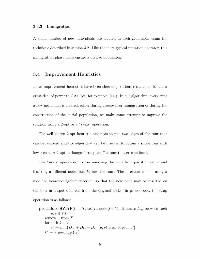
The “swap” operation involves removing the node from partition set Vi and

inserting a different node from Vi into the tour. The insertion is done using a

modified nearest-neighbor criterion, so that the new node may be inserted on

the tour in a spot different from the original node. In pseudocode, the swap

operation is as follows:

procedure SWAP(tour T , set Vi, node j ∈ Vi, distances Duv between eachu, v ∈ V )

remove j from Tfor each k ∈ Vi

ck ← min{Duk + Dkv −Duv|(u, v) is an edge in T}k∗ ← argmink∈Vi

{ck}

8

insert k∗ into T between the nodes u and v that attained the cost ck∗

Note that k∗ may be the same node as j, which allows the heuristic to move a

node to a different spot on the tour.

The 2-opt and swap operations are considered separately by our heuristic;

they are not integrated, as in the G2-opt, G3-opt, and G-opt methods used by

[20].

When an improvement is made to the solution, the encoding must be altered

to reflect the new tour. We do this by rearranging the fractional parts of the

genes to give rise to the new tour. When a swap is performed, we must also

adjust the integer part of the gene for the affected set.

To take a simple example, suppose we have the chromosome

1.1 1.3 1.4 1.7

for the sets Vi given in section 3.1; this represents the tour 1 → 6 → 11 →

16. Now suppose we perform a swap by replacing node 16 with node 17 and

repositioning it after node 1 so that the new tour is 1 → 17 → 6 → 11. The new

encoding is

1.1 1.4 1.7 2.3.

For each individual in the population, we store both the original (pre-improve-

ment) cost and the final cost after improvements have been made. When a new

individual is created, we compare its cost to the pre-improvement cost of the

individual at position p×N in the previous population, where p ∈ [0, 1] is a pa-

rameter of the algorithm. If the new solution is worse than the pre-improvement

9

cost of this individual we use level-I improvement: apply one 2-opt exchange

and one swap (assuming a profitable one can be found) and store the resulting

individual. If, on the other hand, the new solution is better, we use level-II

improvement: apply 2-opts until no profitable 2-opts can be found, then apply

swaps until no profitable swaps can be found, and repeat until no improvements

have been made in a given pass. In both cases, we use a “first-improving” strat-

egy in which the first improvement of a given type that improves the objective

value is implemented, rather than searching for the best such improvement before

choosing one.

This technique is designed to spend more time improving solutions that seem

promising in comparison to previous solutions and to spend less time on the

others. We use p = 0.05 in our implementation.

No improvement is done during the reproduction phase, since these solutions

have already been improved. During the construction of the initial population,

we first create and sort all of the individuals, and then apply level-II improvement

to the best p×N solutions and level-I improvement to the rest.

3.5 Population Management

Two issues are worth mentioning regarding how we maintain GA populations.

First, no duplicates are allowed in the population. Each time a new individ-

ual is created, it is compared to the individuals already in the population; if it

matches one of them, it is discarded and a new individual is created. Duplicate-

10

checking is performed after improvement, and individuals are considered identi-

cal if the decoded solutions are identical, not the genes. That is, chromosomes

2.14 4.25 3.50 2.68 and 2.07 4.73 3.81 2.99 are considered identical since they

represent the same tour.

Second, it is undesirable to allow multiple “reflections” and “rotations” of

a tour to co-exist in the population. That is, if 1 → 6 → 11 → 16 is in the

population, we would not want 6 → 11 → 16 → 1 or 16 → 11 → 6 → 1 in the

population. There are two reasons for this. One is that such quasi-duplicates

appear to add diversity to the population but in fact do not, and so should be

avoided just as duplicates are.

The second reason is that crossover between two such individuals will result

in offspring whose genetic information is “watered down” and may lead to slower

convergence of the GA. In the course of the GA, nodes that should be at the

beginning of the tour tend to evolve fractional parts of the gene that are close

to 0; others evolve fractions close to 1. For this process to work, we need a firm

notion of “the beginning of the tour”—that is, we can’t allow reflections and

rotations.

To avoid rotations, we artificially set the fractional part of the gene for V1 to

0, ensuring that set 1 will be at the beginning of the tour. To avoid reflections,

we must choose between the two orderings of a given tour that begin at set 1.

The node from V1 has two neighbors; we require the lower-indexed neighbor to

appear in slot 2 on the tour (and the higher-indexed neighbor to appear in slot

m). These rules ensure that each tour is stored in a unique manner and that

11

quasi-duplicates are eliminiated.

3.6 Termination Criteria

The algorithm terminates when 250 iterations have been executed, or when 10

consecutive iterations have failed to improve the best-known solution. (These

numbers are parameters that may easily be changed.)

4 Computational Results

Fischetti, Gonzalez, and Toth [7] describe a branch-and-cut algorithm to solve

the GTSP. In their paper, they derive test problems by applying a partitioning

method to 46 standard TSP instances from the TSPLIB library [19]. They pro-

vide optimal objective values for each of the problems, and since the partitioning

method is deterministic and is described in enough detail to reproduce their test

problems, we were able to apply our heuristic to the same problems and compare

the results.

We tested our algorithm on all of the problems disussed in [7] except the five

problems that use great-circle (geographical) distances. The problems we tested

have between 48 and 442 nodes; m is set to dn/5e in each case, where n is the

number of nodes and m is the number of clusters. Most of the problems use

Euclidean distances, but a few have explicit distance matrices given,2 and one2The explicit distance matrices do not satisfy the triangle inequality. Nevertheless, the optimal solutions

to the GTSP for these problems contain exactly one node per set, allowing us to use the results from [7].

12

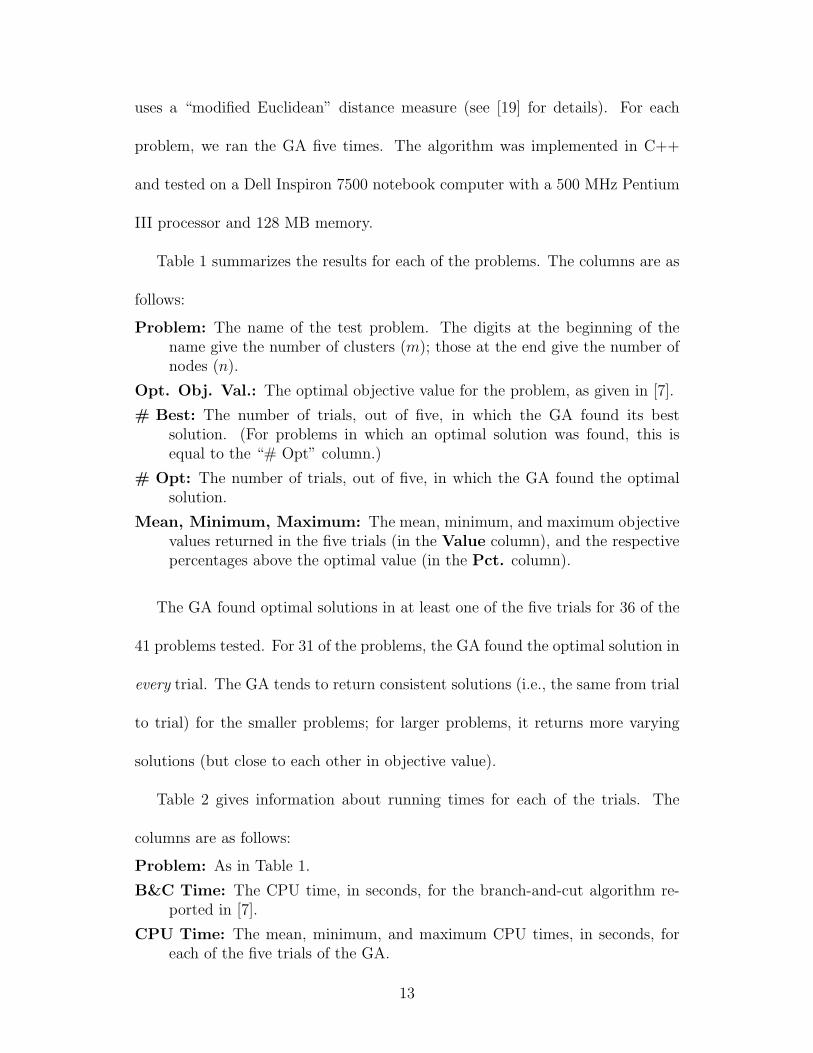
uses a “modified Euclidean” distance measure (see [19] for details). For each

problem, we ran the GA five times. The algorithm was implemented in C++

and tested on a Dell Inspiron 7500 notebook computer with a 500 MHz Pentium

III processor and 128 MB memory.

Table 1 summarizes the results for each of the problems. The columns are as

follows:

Problem: The name of the test problem. The digits at the beginning of thename give the number of clusters (m); those at the end give the number ofnodes (n).

Opt. Obj. Val.: The optimal objective value for the problem, as given in [7].

# Best: The number of trials, out of five, in which the GA found its bestsolution. (For problems in which an optimal solution was found, this isequal to the “# Opt” column.)

# Opt: The number of trials, out of five, in which the GA found the optimalsolution.

Mean, Minimum, Maximum: The mean, minimum, and maximum objectivevalues returned in the five trials (in the Value column), and the respectivepercentages above the optimal value (in the Pct. column).

The GA found optimal solutions in at least one of the five trials for 36 of the

41 problems tested. For 31 of the problems, the GA found the optimal solution in

every trial. The GA tends to return consistent solutions (i.e., the same from trial

to trial) for the smaller problems; for larger problems, it returns more varying

solutions (but close to each other in objective value).

Table 2 gives information about running times for each of the trials. The

columns are as follows:

Problem: As in Table 1.

B&C Time: The CPU time, in seconds, for the branch-and-cut algorithm re-ported in [7].

CPU Time: The mean, minimum, and maximum CPU times, in seconds, foreach of the five trials of the GA.

13

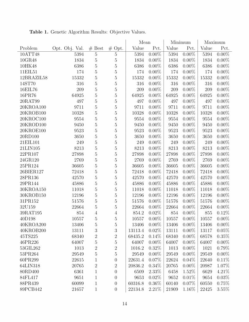
Table 1. Genetic Algorithm Results: Objective Values.

Mean Minimum MaximumProblem Opt. Obj. Val. # Best # Opt. Value Pct. Value Pct. Value Pct.10ATT48 5394 5 5 5394 0.00% 5394 0.00% 5394 0.00%10GR48 1834 5 5 1834 0.00% 1834 0.00% 1834 0.00%10HK48 6386 5 5 6386 0.00% 6386 0.00% 6386 0.00%11EIL51 174 5 5 174 0.00% 174 0.00% 174 0.00%12BRAZIL58 15332 5 5 15332 0.00% 15332 0.00% 15332 0.00%14ST70 316 5 5 316 0.00% 316 0.00% 316 0.00%16EIL76 209 5 5 209 0.00% 209 0.00% 209 0.00%16PR76 64925 5 5 64925 0.00% 64925 0.00% 64925 0.00%20RAT99 497 5 5 497 0.00% 497 0.00% 497 0.00%20KROA100 9711 5 5 9711 0.00% 9711 0.00% 9711 0.00%20KROB100 10328 5 5 10328 0.00% 10328 0.00% 10328 0.00%20KROC100 9554 5 5 9554 0.00% 9554 0.00% 9554 0.00%20KROD100 9450 5 5 9450 0.00% 9450 0.00% 9450 0.00%20KROE100 9523 5 5 9523 0.00% 9523 0.00% 9523 0.00%20RD100 3650 5 5 3650 0.00% 3650 0.00% 3650 0.00%21EIL101 249 5 5 249 0.00% 249 0.00% 249 0.00%21LIN105 8213 5 5 8213 0.00% 8213 0.00% 8213 0.00%22PR107 27898 5 5 27898 0.00% 27898 0.00% 27898 0.00%24GR120 2769 5 5 2769 0.00% 2769 0.00% 2769 0.00%25PR124 36605 5 5 36605 0.00% 36605 0.00% 36605 0.00%26BIER127 72418 5 5 72418 0.00% 72418 0.00% 72418 0.00%28PR136 42570 5 5 42570 0.00% 42570 0.00% 42570 0.00%29PR144 45886 5 5 45886 0.00% 45886 0.00% 45886 0.00%30KROA150 11018 5 5 11018 0.00% 11018 0.00% 11018 0.00%30KROB150 12196 5 5 12196 0.00% 12196 0.00% 12196 0.00%31PR152 51576 5 5 51576 0.00% 51576 0.00% 51576 0.00%32U159 22664 5 5 22664 0.00% 22664 0.00% 22664 0.00%39RAT195 854 4 4 854.2 0.02% 854 0.00% 855 0.12%40D198 10557 5 5 10557 0.00% 10557 0.00% 10557 0.00%40KROA200 13406 5 5 13406 0.00% 13406 0.00% 13406 0.00%40KROB200 13111 3 3 13113.4 0.02% 13111 0.00% 13117 0.05%45TS225 68340 2 2 68435.2 0.14% 68340 0.00% 68578 0.35%46PR226 64007 5 5 64007 0.00% 64007 0.00% 64007 0.00%53GIL262 1013 2 2 1016.2 0.32% 1013 0.00% 1021 0.79%53PR264 29549 5 5 29549 0.00% 29549 0.00% 29549 0.00%60PR299 22615 1 0 22631.4 0.07% 22624 0.04% 22640 0.11%64LIN318 20765 2 2 20836.2 0.34% 20765 0.00% 20987 1.07%80RD400 6361 1 0 6509 2.33% 6458 1.52% 6629 4.21%84FL417 9651 1 0 9653 0.02% 9652 0.01% 9654 0.03%88PR439 60099 1 0 60316.8 0.36% 60140 0.07% 60550 0.75%89PCB442 21657 1 0 22134.8 2.21% 21909 1.16% 22425 3.55%

14

# Iterations: The mea, minimum, and maximum number of iterations beforethe GA terminated.

# Impr. Iter.: The mean, minimum, and maximum number of iterations dur-ing which the GA found a new solution better than the current best solution.

The branch-and-cut times are provided only for reference; no direct compar-

ison is possible since the two algorithms were developed and run on different

machines. Nevertheless, it is clear that the running times of the GA are compet-

itive with the branch-and-cut times for smaller problems, and much shorter for

the larger problems. Furthermore, the GA generally found its best solution in

the first few iterations and spent most of the iterations waiting to terminate.

Note that the GA seems to perform equally well for problems with modi-

fied Euclidean distances (10ATT48), and explicit distances (10GR48, 10HK48,

12BRAZIL5, and 24GR120) as it does for those with Euclidean distances. We

were unable to test problems with non-geographic clusters (for example, in which

nodes are grouped randomly) since no optimal objective values have been pub-

lished for such problems.

In general, the bulk of the running time (well over 95% for the larger problems)

is spent in the improvement heuristic, suggesting that a more efficient improve-

ment method (such as Renaud and Boctor’s G2-opt or G3-opt) may improve the

speed of the GA even more.

For the sake of comparison, Table 3 compares the performance of the GA

heuristic with that of two others on the same TSPLIB problems. The first is

the GI3 heuristic proposed by Renaud and Boctor [20]; the second is Noon’s

generalized nearest neighbor heuristic [16] combined with the improvement phase

15

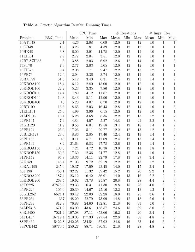
Table 2. Genetic Algorithm Results: Running Times.

CPU Time # Iterations # Impr. Iter.Problem B&C Time Mean Min Max Mean Min Max Mean Min Max10ATT48 2.1 4.26 2.08 6.09 12.0 12 12 1.0 1 110GR48 1.9 3.25 1.81 4.39 12.0 12 12 1.0 1 110HK48 3.8 6.00 2.91 14.78 12.0 12 12 1.0 1 111EIL51 2.9 2.77 2.04 3.51 12.0 12 12 1.0 1 112BRAZIL58 3 3.88 2.03 6.92 12.6 12 14 1.6 1 314ST70 7.3 2.77 2.03 5.05 12.0 12 12 1.0 1 116EIL76 9.4 2.08 1.71 2.47 12.2 12 13 1.2 1 216PR76 12.9 2.94 2.36 3.74 12.0 12 12 1.0 1 120RAT99 51.5 5.12 3.40 6.31 12.4 12 13 1.4 1 220KROA100 18.4 6.12 2.80 15.00 12.0 12 12 1.0 1 120KROB100 22.2 5.23 3.35 7.86 12.0 12 12 1.0 1 120KROC100 14.4 7.89 4.12 11.87 12.0 12 12 1.0 1 120KROD100 14.3 8.43 5.11 12.96 12.0 12 12 1.0 1 120KROE100 13 5.20 4.07 6.70 12.0 12 12 1.0 1 120RD100 16.6 8.65 2.03 16.43 12.8 12 14 1.6 1 321EIL101 25.6 4.99 3.96 6.15 12.0 12 12 1.0 1 121LIN105 16.4 5.28 3.68 8.35 12.2 12 13 1.2 1 222PR107 7.4 4.84 4.07 5.27 14.8 12 22 2.2 1 324GR120 41.9 9.56 6.04 12.58 13.4 12 18 1.4 1 225PR124 25.9 17.23 5.11 29.77 12.2 12 13 1.2 1 226BIER127 23.6 8.86 2.85 17.46 12.4 12 13 1.4 1 228PR136 43 10.11 5.71 17.69 12.4 12 13 1.4 1 229PR144 8.2 21.64 9.83 47.78 12.6 12 14 1.4 1 230KROA150 100.3 7.24 4.72 10.38 13.0 12 14 1.8 1 230KROB150 60.6 17.30 12.36 24.77 12.8 12 14 1.6 1 231PR152 94.8 18.36 14.11 22.79 17.8 13 27 3.4 2 532U159 146.4 21.03 9.72 32.19 12.2 12 13 1.2 1 239RAT195 245.9 19.37 17.09 23.45 14.0 12 15 2.4 1 340D198 763.1 32.27 11.32 59.42 15.2 12 20 2.2 1 440KROA200 187.4 23.12 16.42 36.91 14.0 13 16 2.2 2 340KROB200 268.5 19.62 13.78 25.87 20.8 13 28 4.4 2 645TS225 37875.9 29.33 16.31 41.30 18.8 15 28 4.0 3 546PR226 106.9 20.39 14.67 25.16 12.2 12 13 1.2 1 253GIL262 6624.1 33.42 22.03 52.28 18.0 13 25 3.6 1 753PR264 337 48.29 22.79 73.99 14.8 12 18 2.6 1 560PR299 812.8 76.88 24.60 132.81 21.8 16 33 5.0 3 664LIN318 1671.9 83.90 43.61 158.57 24.6 15 39 5.0 3 880RD400 7021.4 197.08 87.11 353.66 16.2 12 20 3.4 1 584FL417 16719.4 210.05 177.30 277.54 22.8 15 38 4.8 2 888PR439 5422.8 342.25 234.54 457.92 24.6 16 33 4.6 3 689PCB442 58770.5 250.27 88.71 486.91 21.8 14 28 4.8 2 8

16

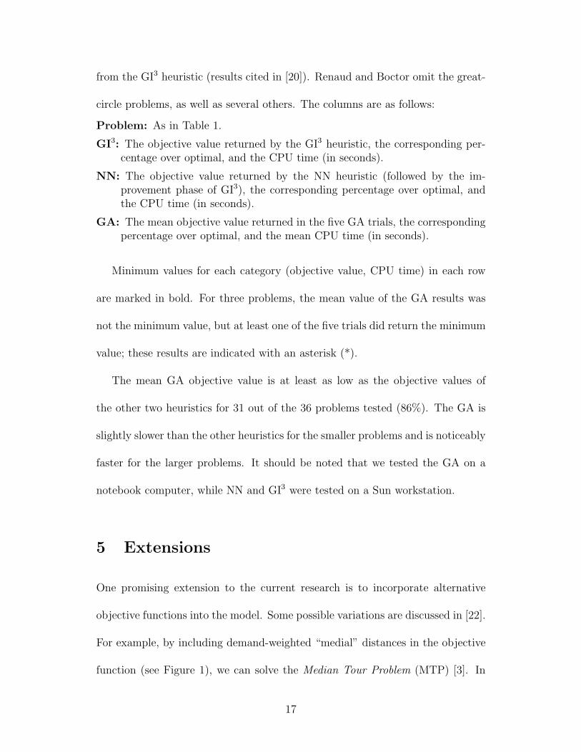
from the GI3 heuristic (results cited in [20]). Renaud and Boctor omit the great-

circle problems, as well as several others. The columns are as follows:

Problem: As in Table 1.

GI3: The objective value returned by the GI3 heuristic, the corresponding per-centage over optimal, and the CPU time (in seconds).

NN: The objective value returned by the NN heuristic (followed by the im-provement phase of GI3), the corresponding percentage over optimal, andthe CPU time (in seconds).

GA: The mean objective value returned in the five GA trials, the correspondingpercentage over optimal, and the mean CPU time (in seconds).

Minimum values for each category (objective value, CPU time) in each row

are marked in bold. For three problems, the mean value of the GA results was

not the minimum value, but at least one of the five trials did return the minimum

value; these results are indicated with an asterisk (*).

The mean GA objective value is at least as low as the objective values of

the other two heuristics for 31 out of the 36 problems tested (86%). The GA is

slightly slower than the other heuristics for the smaller problems and is noticeably

faster for the larger problems. It should be noted that we tested the GA on a

notebook computer, while NN and GI3 were tested on a Sun workstation.

5 Extensions

One promising extension to the current research is to incorporate alternative

objective functions into the model. Some possible variations are discussed in [22].

For example, by including demand-weighted “medial” distances in the objective

function (see Figure 1), we can solve the Median Tour Problem (MTP) [3]. In

17

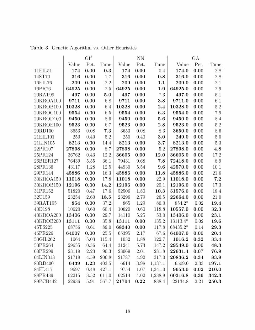
Table 3. Genetic Algorithm vs. Other Heuristics.

GI3 NN GAValue Pct. Time Value Pct. Time Value Pct. Time

11EIL51 174 0.00 0.3 174 0.00 0.4 174.0 0.00 2.814ST70 316 0.00 1.7 316 0.00 0.8 316.0 0.00 2.816EIL76 209 0.00 2.2 209 0.00 1.1 209.0 0.00 2.116PR76 64925 0.00 2.5 64925 0.00 1.9 64925.0 0.00 2.920RAT99 497 0.00 5.0 497 0.00 7.3 497.0 0.00 5.120KROA100 9711 0.00 6.8 9711 0.00 3.8 9711.0 0.00 6.120KROB100 10328 0.00 6.4 10328 0.00 2.4 10328.0 0.00 5.220KROC100 9554 0.00 6.5 9554 0.00 6.3 9554.0 0.00 7.920KROD100 9450 0.00 8.6 9450 0.00 5.6 9450.0 0.00 8.420KROE100 9523 0.00 6.7 9523 0.00 2.8 9523.0 0.00 5.220RD100 3653 0.08 7.3 3653 0.08 8.3 3650.0 0.00 8.621EIL101 250 0.40 5.2 250 0.40 3.0 249.0 0.00 5.021LIN105 8213 0.00 14.4 8213 0.00 3.7 8213.0 0.00 5.322PR107 27898 0.00 8.7 27898 0.00 5.2 27898.0 0.00 4.825PR124 36762 0.43 12.2 36605 0.00 12.0 36605.0 0.00 17.226BIER127 76439 5.55 36.1 79431 9.68 7.8 72418.0 0.00 8.928PR136 43117 1.28 12.5 44930 5.54 9.6 42570.0 0.00 10.129PR144 45886 0.00 16.3 45886 0.00 11.8 45886.0 0.00 21.630KROA150 11018 0.00 17.8 11018 0.00 22.9 11018.0 0.00 7.230KROB150 12196 0.00 14.2 12196 0.00 20.1 12196.0 0.00 17.331PR152 51820 0.47 17.6 52506 1.80 10.3 51576.0 0.00 18.432U159 23254 2.60 18.5 23296 2.79 26.5 22664.0 0.00 21.039RAT195 854 0.00 37.2 865 1.29 86.0 854.2* 0.02 19.440D198 10620 0.60 60.4 10620 0.60 118.8 10557.0 0.00 32.340KROA200 13406 0.00 29.7 14110 5.25 53.0 13406.0 0.00 23.140KROB200 13111 0.00 35.8 13111 0.00 135.2 13113.4* 0.02 19.645TS225 68756 0.61 89.0 68340 0.00 117.8 68435.2* 0.14 29.346PR226 64007 0.00 25.5 65395 2.17 67.6 64007.0 0.00 20.453GIL262 1064 5.03 115.4 1032 1.88 122.7 1016.2 0.32 33.453PR264 29655 0.36 64.4 31241 5.73 147.2 29549.0 0.00 48.360PR299 23119 2.23 90.3 23069 2.01 281.8 22631.4 0.07 76.964LIN318 21719 4.59 206.8 21787 4.92 317.0 20836.2 0.34 83.980RD400 6439 1.23 403.5 6614 3.98 1,137.1 6509.0 2.33 197.184FL417 9697 0.48 427.1 9754 1.07 1,341.0 9653.0 0.02 210.088PR439 62215 3.52 611.0 62514 4.02 1,238.9 60316.8 0.36 342.389PCB442 22936 5.91 567.7 21704 0.22 838.4 22134.8 2.21 250.3

18

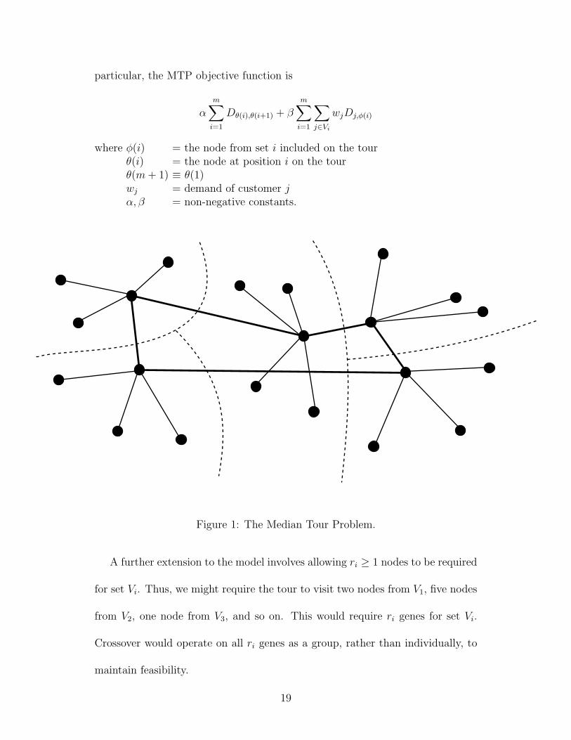
particular, the MTP objective function is

αm

∑

i=1

Dθ(i),θ(i+1) + βm

∑

i=1

∑

j∈Vi

wjDj,φ(i)

where φ(i) = the node from set i included on the tourθ(i) = the node at position i on the tourθ(m + 1) ≡ θ(1)wj = demand of customer jα, β = non-negative constants.

Figure 1: The Median Tour Problem.

A further extension to the model involves allowing ri ≥ 1 nodes to be required

for set Vi. Thus, we might require the tour to visit two nodes from V1, five nodes

from V2, one node from V3, and so on. This would require ri genes for set Vi.

Crossover would operate on all ri genes as a group, rather than individually, to

maintain feasibility.

19

In addition, we could incorporate a fixed cost for including a customer on the

tour, although, as mentioned earlier, this can also be accomplished through a

transformation of the distance matrix. With the variations mentioned so far, we

could, through a suitable choice of parameters, model a wide range of location,

routing, and location/routing problems, including the TSP, MTP, and P -median

problems. (To obtain the P -median problem, we set α = 0, m = 1 [all nodes in

the same cluster], and r1 = P .)

Another appealing extension is to allow the tour to include more than the

required number of nodes in each cluster. (If the triangle inequality does not

hold, it may be advantageous to visit more than the required number.) This

would capture the more general form of the GTSP and would, with the extensions

mentioned above, allow an even richer variety of problems, including the fixed-

charge facility location problem (again, set α = 0, m = 1). It would, however,

require a more complicated encoding scheme and GA operators, since the number

of genes would vary from generation to generation as the number of open facilities

changes from one solution to the next.

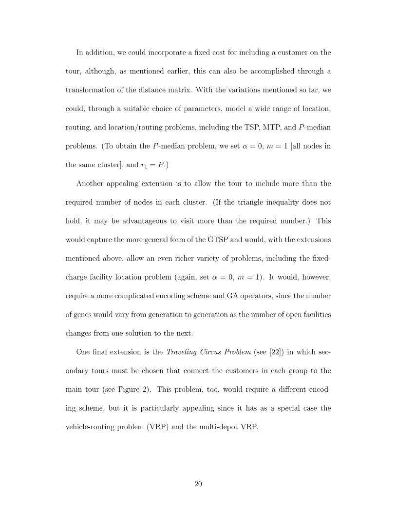
One final extension is the Traveling Circus Problem (see [22]) in which sec-

ondary tours must be chosen that connect the customers in each group to the

main tour (see Figure 2). This problem, too, would require a different encod-

ing scheme, but it is particularly appealing since it has as a special case the

vehicle-routing problem (VRP) and the multi-depot VRP.

20

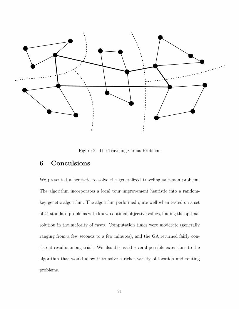
Figure 2: The Traveling Circus Problem.

6 Conculsions

We presented a heuristic to solve the generalized traveling salesman problem.

The algorithm incorporates a local tour improvement heuristic into a random-

key genetic algorithm. The algorithm performed quite well when tested on a set

of 41 standard problems with known optimal objective values, finding the optimal

solution in the majority of cases. Computation times were moderate (generally

ranging from a few seconds to a few minutes), and the GA returned fairly con-

sistent results among trials. We also discussed several possible extensions to the

algorithm that would allow it to solve a richer variety of location and routing

problems.

21

References

[1] Bean, J. C. 1994. Genetic Algorithms and Random Keys for Sequencing and

Optimization. ORSA J. Comput. 6, 154–160.

[2] Chentsov, A. G., and L. N. Korotayeva. 1997. The Dynamic Programming

Method in the Generalized Traveling Salesman Problem. Math. Comput.

Model. 25, 93–105.

[3] Current, J. R., and D. A. Schilling. 1994. The Median Tour and Maximal

Covering Tour Problems: Formulations and Heuristics. Eur. J. Opnl. Res.

73, 114–126.

[4] Dimitrijevic, V, and Z. Saric. 1997. An Efficient Transformation of the Gen-

eralized Traveling Salesman Problem into the Traveling Salesman Problem

on Digraphs. Inform. Sci. 102, 105–110.

[5] Dror, M., and A. Langevin. 1997. A Generalized Traveling Salesman Problem

Approach to the Directed Clustered Rural Postman Problem. Transp. Sci.

31, 187–192.

[6] Fischetti, M., J. J. S. Gonzalez and P. Toth. 1995. The Symmetrical Gener-

alized Traveling Salesman Polytope. Networks. 26, 113–123.

[7] Fischetti, M., J. J. S. Gonzalez, and P. Toth. 1997. A Branch-and-Cut Al-

gorithm for the Symmetric Generalized Traveling Salesman Problem. Opns.

Res. 45, 378–394.

22

[8] Henry-Labordere, A. L. 1969. The Record Balancing Problem: A Dynamic

Programming Solution of a Generalized Traveling Salesman Problem. RIRO.

B-2, 43–49.

[9] Laporte, G., A. Asef-Vaziri and C. Sriskandarajah. 1996. Some Applications

of the Generalized Travelling Salesman Problem. J. Opnl. Res. Soc. 47,

1461–1467.

[10] Laporte, G., H. Mercure and Y. Nobert. 1985. Finding the Shortest Hamil-

tonian Circuit through n Clusters: A Lagrangean Approach. Congressus

Numerantium. 48, 277–290.

[11] Laporte, G., H. Mercure and Y. Nobert. 1987. Generalized Traveling Sales-

man Problem through n Sets of Nodes: The Asymmetrical Case. Discr.

Appl. Math. 18, 185–197.

[12] Laporte, G., and Y. Nobert. 1983. Generalized Traveling Salesman Problem

through n Sets of Nodes: An Integer Programming Approach. INFOR. 21,

61–75.

[13] Laporte, G., and F. Semet. 1999. Computational Evaluation of a Transfor-

mation Procedure for the Symmetric Generalized Traveling Salesman Prob-

lem. INFOR. 37, 114–120.

[14] Levine, D. 1996. Application of a Hybrid Genetic Algorithm to Airline Crew

Scheduling. Comput. Opns. Res. 23, 547–558.

[15] Lien, Y. N., E. Ma, and B. W. S. Wah. 1993. Transformation of the Gen-

eralized Traveling-Salesman Problem into the Standard Traveling-Salesman

23

Problem. Inform. Sci. 74, 177–189.

[16] Noon, C. E. 1988. The Generalized Traveling Salesman Problem. Unpub-

lished Dissertation, Department of Industrial and Operations Engineering,

The University of Michigan, Ann Arbor.

[17] Noon, C. E., and J. C. Bean. 1991. A Lagrangian Based Approach for the

Asymmetric Generalized Traveling Salesman Problem. Opns. Res. 39, 623–

632.

[18] Noon, C. E., and J. C. Bean. 1993 An Efficient Transformation of the Gen-

eralized Traveling Salesman Problem. INFOR. 31, 39–44.

[19] Reinelt, G. 1991. TSPLIB—A Traveling Salesman Problem Library. ORSA

J. Comput. 3, 376–384.

[20] Renaud, J., and F. F. Boctor. 1998. An Efficient Composite Heuristic for

the Symmetric Generalized Traveling Salesman Problem. Eur. J. Opnl. Res.

108, 571–584.

[21] Renaud, J., F. F. Boctor, and G. Laporte. 1996. A Fast Composite Heuristic

for the Symmetric Traveling Salesman Problem. INFORMS J. Comput. 4,

134–143.

[22] ReVelle, C. S., and G. Laporte. 1996. The Plant Location Problem: New

Models and Research Prospects. Opns. Res. 44, 864–874.

[23] Saskena, J. P. 1970. Mathematical Model of Scheduling Clients Through

Welfare Agencies. J. Canadian Oper. Res. Soc. 8, 185–200.

24

[24] Spears, W. M., and K. A. DeJong. 1991. On the Virtues of Paremeterized

Uniform Crossover. Proceedings of the Fourth International Conference on

Genetic Algorithms. 230–236.

[25] Srivastava, S. S., S. Kumar, R. C. Garg and P. Sen. 1969. Generalized Trav-

eling Salesman Problem Through n Sets of Nodes. J. Canadian Oper. Res.

Soc. 97–101.

25