A Radio-Frequency Tool for Planning Wireless

Sensor Networks

Gerardo Di Martino, Antonio Iodice, Daniele Riccio, Giuseppe Ruello

Department of Electric Engineering and Information Technology,

Università degli Studi di Napoli Federico II

Naples, Italy

gerardo.dimartino@unina.it ; iodice@unina.it ; daniele.riccio@unina.it ; ruello@unina.it

Abstract— We present a software tool able to help planning

and deployment of wireless sensor networks (WSN) in an outdoor

environment. The tool is based on a ray-tracing algorithm for the

evaluation of electromagnetic propagation in a built-up area, and

on additional software modules that use the output of the

electromagnetic solver to generate nodes’ connectivity matrix, to

compute individual nodes' coverage areas, and to identify the

best locations where gateways can be placed. The presented tool

is able to deal with the radio-frequency propagation issues

involved in WSN planning and deployment, and it is conceived as

a part of an overall WSN deployment, planning, and

commissioning & maintenance tool that is being developed in the

framework of a European project.

Keywords—Wireless sensor networks; electromagnetic wave

propagation.

I. INTRODUCTION

Wireless sensor networks (WSN) are employed in a wide range of applications, and have been the subject of considerable research. However, in spite of that, large scale application of this technology is still limited by technical complexity and cost issues. In particular, among other issues, the planning phase is very expensive, because it requires that connectivity, coverage, cost, network longevity, and service quality are all considered. In addition, predicting WSN performance before its real deployment is very challenging, so that costly trial-and-error procedures are usually employed.

In this framework, simulation tools may be very helpful to WSN designers. In fact, currently many wireless network simulation tools are publicly available, among which, for instance, OMNeT++ [1], TOSSIM [2]. However, all of them rely on very simple, heuristic propagation models that do not account for the detailed description of the surrounding environment and obstacles. On the other hand, electromagnetic propagation prediction tools accounting for complex outdoor environment do exist, see for instance [3]-[6]. However, they are tailored for radio and television broadcasting or cellular telephony systems, or Wi-Fi, and have not been employed in the framework of WSN planning.

In this work we present a software tool able to help planning and deployment of WSN in a complex outdoor

environment. The core of the tool is an electromagnetic solver that employs a ray-tracing algorithm for the evaluation of electromagnetic propagation in a built-up area. It is substantially based on the methods described in [5]-[6], with some modifications to tailor it to the WSN case and to adapt the format of input and output to more widespread standards. This electromagnetic solver allows computation of the electromagnetic field in a built-up area, when the three-dimensional (3-D) topography (terrain height profile and buildings) of the considered city area is prescribed, as well as the radiating sources (locations, input power and antenna radiation diagram of WSN nodes). The solver considers both reflected and diffracted rays, although a “fast mode” only considering reflected rays may be also selected. The output of the solver is the electromagnetic field intensity on a 3-D grid in the considered area: it can be directly displayed to the WSN designer, or it can be provided as an input to additional software modules that use it to generate nodes’ connectivity matrix, to compute individual node’s coverage areas, and to identify the best locations where gateways can be placed, according to different WSN planning scenarios, as described in the next sections.

The presented tool is able to deal with the radio-frequency (RF) propagation issues involved in WSN planning and deployment, so that in the following we will refer to it as "RF tool". However, it is conceived as a part of an overall WSN deployment, planning, and commissioning & maintenance (DPCM) tool that is being developed in the framework of a European project [7]. In particular, the RF tool is directly interfaced with a Graphic User Interface (GUI) and with a network simulator, which takes care about protocols, data throughput, etc.

II. RF TOOL DESCRIPTION

The proposed RF tool is composed of an electromagnetic solver and of three additional modules, namely a "connectivity matrix" module, a "coverage" module, and a "gateway positioning" module.

A. Electromagnetic solver

The electromagnetic solver input is a digital description of the scene and of the transmitting antenna. The scene

This work has been supported by the ARTEMIS Joint Undertaking (EU) and by the Italian Ministry of University and Scientific Research, within the

WSN - DPCM project.

description is provided by a file in kml (Keyhole Markup Language) format describing the buildings, and a raster file describing the terrain topography (Digital Terrain Model, DTM). The format employed for the buildings' description makes it very easy to get built up area geometrical information even when it is not possible, or not economical, to obtain it from local authorities. In fact, kml files describing buildings can be obtained from Google Map or Google Earth images, or also from aerial photography by using the algorithm of [8]. However, accuracy of scene description certainly affects the solver prediction results. Buildings' walls and terrain relative permittivity and conductivity can be also stored to account for the electromagnetic properties. However, this information is seldom available, and default values can be selected according to the area typology (historical area, residential area, business district). Antenna description is provided by means of its position and pointing, radiated power, polarization and radiation diagram.

Our solver is based on a 3D space analysis similar to that of [5]-[6]. A ray-tracing algorithm is employed that considers direct, reflected and diffracted rays. Reflections are treated by using Geometrical Optics (GO), whereas diffraction is evaluated by using the Uniform Theory of Diffraction (UTD). Since most of the computational load is due to diffracted rays, the user can optionally select a "fast mode" that only considers direct and reflected rays.

The solver output is a 3-D map of the field levels produced by the transmitting antenna in the considered area. In fact, the electromagnetic field is computed on regular 2-D grids ("layers") placed on surfaces at different fixed heights above the ground (or above the roof, if the grid point is in correspondence of a building). This output is stored in a geotiff format file, and can be displayed by the GUI and/or passed to the additional software modules.

B. Connectivity matrix module

This module takes N simulated field maps produced by the electromagnetic solver and extracts the field values radiated by each antenna (node) at the locations of all other antennas (nodes). A "connectivity matrix" is then obtained, which is stored in a json (JavaScript Object Notation) file. If desired, and if a receiver field threshold level is defined, this matrix can be immediately translated into a binary matrix whose non-zero elements can be displayed by the GUI as arcs connecting corresponding nodes (see Section IV).

C. Coverage module

This simple module, by using the field map relative to a transmitting node, produced by the electromagnetic solver, and given a receiver threshold, computes the coverage area of the considered node, stored as the list of output grid points for which the field level is higher than the receiver threshold. The coverage area can be displayed by the GUI.

D. Gateway positioning module

Inputs of this module are N simulated field maps produced by the electromagnetic solver (one for each transmitting node) and a gateway receiver threshold. First of all, the module finds

the grid points, if any, for which all the N field levels are higher than the threshold. These are "candidate points" for the gateway positioning. Among these points, the module determines the best gateway position by using one of the following criteria, selectable by the user.

"Median" criterion: the grid point such that the median value of the N field levels is the highest is chosen.

"90%" criterion: for each grid point, the field value exceeded by the 90% of the N field levels is computed; the grid point such that this value is the highest is chosen.

"Minimum" criterion: the grid point such that the minimum of the N field levels is the highest is chosen.

If no candidate point is found, the set of N nodes is split into different subsets (clusters) such that for each subset at least one candidate point is present. For each cluster of nodes, the best gateway position is determined as described above.

III. RF TOOL USAGE

The proposed RF tool may be employed according to three different "functionality modes", which we call "standard", "coverage", and "gateway" modes.

A. Standard mode

This functionality mode can be selected if no strict constraint on motes' positions is imposed by the application, and a mesh topology is used.

Given the 3-D description of the scene, and, possibly, additional information (for instance, what quantity, and where, must be measured by the sensors), the user provides a first guess of the motes positions; he also selects a propagation model among the available ones (fast, with high speed and low accuracy, or standard, with low speed and high accuracy), based on the number of motes. The RF tool (calling solver and connectivity matrix modules) computes the field levels provided by each mote's transmitter in the whole scene and, from these, the output connectivity matrix, see Section II.B. This matrix may be considered by the user to iteratively refine motes' positions and run the RF tool until he/she is satisfied; then the matrix is passed by the RF tool to the network simulator, which verifies that all is in good shape from the viewpoint of data throughput, conflicts, and so on. If necessary, the whole procedure may be iterated.

B. Coverage mode

This functionality mode should be selected if the positions of (few) gateways, or sink nodes, are constrained by, for instance, power availability requirements, and a large number of motes disseminated in the area must be connected with at least one gateway (for instance, think of a large open parking area).

Given the 3-D description of the scene, and given the constraints on the positions of gateways, the user places the (few) gateways (using the GUI) and selects a propagation model among the available ones (see above). In this case, the

standard, high accuracy model can be used. The RF tool (calling solver and coverage modules) computes the field levels provided by each gateway's transmitter in the whole scene and, from these, and from motes' receiver field threshold level, it produces a map of coverage area for each gateway. The motes can be now safely placed in any point belonging to at least one coverage area, and (using solver and connectivity matrix modules) a field level for each mote is computed by the RF tool, along with the connectivity matrix. This matrix may be considered by the user to iteratively refine gateways' positions or transmitted power (if possible at all) and run the RF tool until he/she is satisfied; then the matrix is passed by the RF tool to the "network simulator", which verifies that all is in good shape from the viewpoint of data throughput, conflicts, and so on. If necessary, the whole procedure may be iterated.

C. Gateway mode

This functionality mode should be selected if the positions of motes are constrained by the application (for instance, measurement points are fixed by the object to be measured), and these motes must be connected to one or more gateways or sink nodes, the positions of which are not constrained. However, more in general a similar procedure can be followed if simply one has to add a node, placed in a free position, to an existing network.

Given the 3-D description of the scene, and given the constraints on the positions of motes, the user places the motes (using the GUI) and selects a propagation model among the available ones (see above). The RF tool (solver module) computes the field levels provided by each mote's transmitter in the whole scene. If the gateway's receiver field threshold level is known, the RF tool (gateway module) can verify how many gateways are needed to connect all motes and can suggest the "best" (see section II.D) positions for these gateways. The gateways can be now placed in suggested positions, and a field level for each mote is computed by the RF tool (solver module). Again, a connectivity matrix is therefore generated (connectivity matrix module), and is passed by the RF tool to the "network simulator", which verifies that all is in good shape from the viewpoint of data throughput, conflicts, and so on. If necessary, the whole procedure may be iterated.

TABLE I. SIMULATION RUN PARAMETERS

Parameter Value

Output grid horizontal resolution 5.0 m

Propagation model Standard (GO+UTD)

Nodes' height above ground 1.5 m

Frequency 2.405 GHz

Antenna type Omnidirectional

Antenna transmitted power 1 mW

Receiver threshold 90 dBm

Fig. 1. Google map image of an area in the suburbs of Naples, Italy, with superimposed input building description and WSN nodes' locations.

IV. EXAMPLES

We here consider some examples to illustrate the RF tool capabilities and usage. Let us first consider the standard functionality mode, and suppose that we have to monitor the area shown in Fig. 1. Nine sensor nodes are initially "virtually" placed by using the GUI. The main input parameters are listed in Table I. By using the solver and connectivity matrix modules, the connectivity matrix of Fig.2 is obtained.

Node1 Node2 Node3 Node4 Node5 Node6 Node7 Node8 Node9

Node1 - -72,59 -95,53 -70,59 -97,35 -97,02 -81,36 -86,67 -120,9

Node2 -72,59 - -113,5 -100,9 -74,74 -78,83 -89,31 -114,0 -91,6

Node3 -95,53 -113,5 - -77,49 -74,05 *** -80,01 -94,71 -103,9

Node4 -70,59 -100,9 -77,49 - -93,27 -102,3 *** -113,9 ***

Node5 -97,35 -74,74 -74,05 -93,27 - *** -69,77 -122,1 -109,2

Node6 -97,02 -78,83 *** -102,3 *** - *** *** ***

Node7 -81,36 -89,31 -80,01 *** -69,77 *** - -79,89 ***

Node 8 -86,67 -114,0 -94,71 -113,9 -122,1 *** -79,89 - ***

Node 9 -120,9 -91,68 -103,9 *** -109,2 *** *** *** -

Fig. 2. Connectivity matrix for the scenario of Fig.1. Field levels are expressed in dBm. Asterisks indicate negligible field.

(a) (b)

Fig. 3. Connectivity maps for the scenario of Fig. 1 with 9 (a) and 10 (b) nodes.

Corresponding map is reported in Fig. 3a, where it is evident that node 9 is not connected with the rest of the network. However, by adding a node at a proper position, and using again the RF tool, the connectivity map of Fig. 3b is obtained, in which it is evident that the entire network is connected.

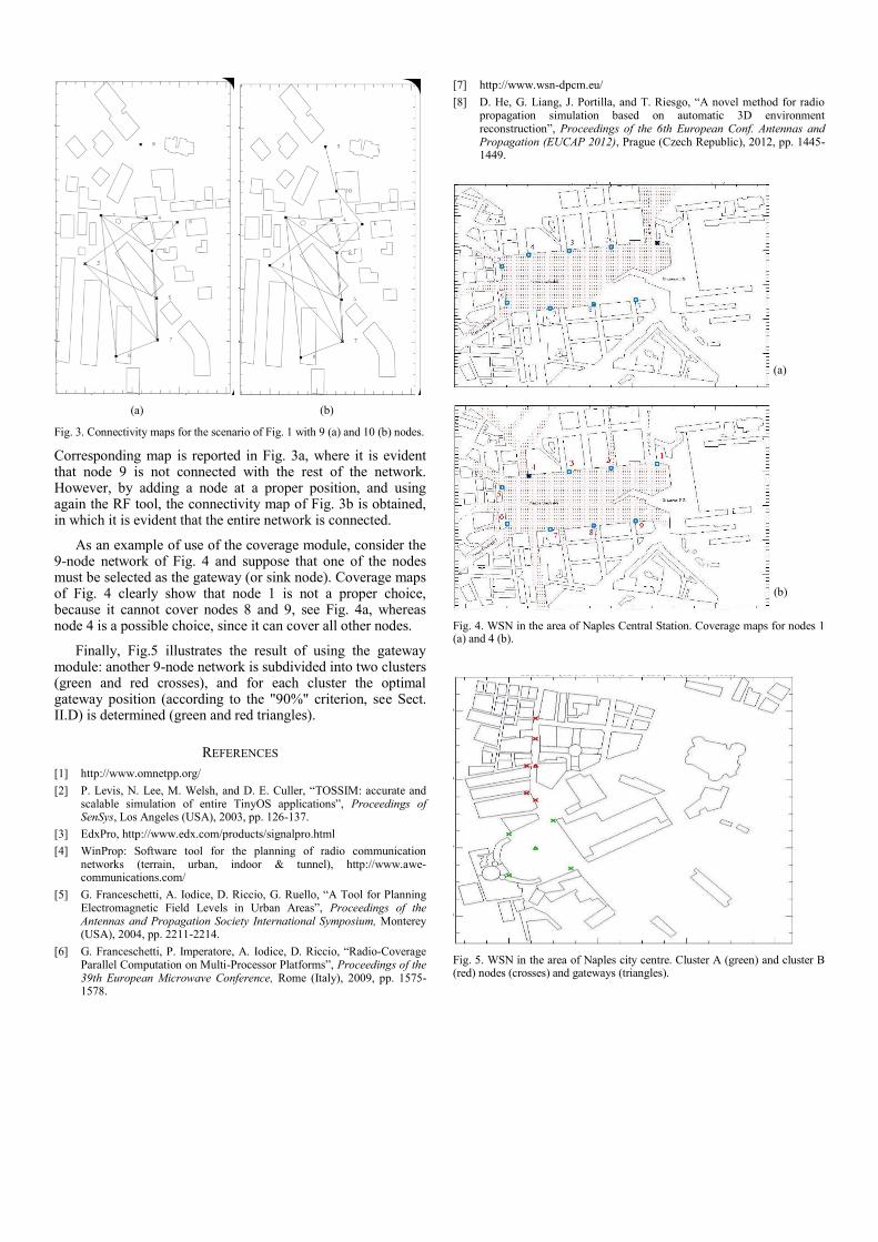
As an example of use of the coverage module, consider the 9-node network of Fig. 4 and suppose that one of the nodes must be selected as the gateway (or sink node). Coverage maps of Fig. 4 clearly show that node 1 is not a proper choice, because it cannot cover nodes 8 and 9, see Fig. 4a, whereas node 4 is a possible choice, since it can cover all other nodes.

Finally, Fig.5 illustrates the result of using the gateway module: another 9-node network is subdivided into two clusters (green and red crosses), and for each cluster the optimal gateway position (according to the "90%" criterion, see Sect. II.D) is determined (green and red triangles).

REFERENCES

[1] http://www.omnetpp.org/

[2] P. Levis, N. Lee, M. Welsh, and D. E. Culler, “TOSSIM: accurate and scalable simulation of entire TinyOS applications”, Proceedings of SenSys, Los Angeles (USA), 2003, pp. 126-137.

[3] EdxPro, http://www.edx.com/products/signalpro.html

[4] WinProp: Software tool for the planning of radio communication networks (terrain, urban, indoor & tunnel), http://www.awe-communications.com/

[5] G. Franceschetti, A. Iodice, D. Riccio, G. Ruello, “A Tool for Planning Electromagnetic Field Levels in Urban Areas”, Proceedings of the Antennas and Propagation Society International Symposium, Monterey (USA), 2004, pp. 2211-2214.

[6] G. Franceschetti, P. Imperatore, A. Iodice, D. Riccio, “Radio-Coverage Parallel Computation on Multi-Processor Platforms”, Proceedings of the 39th European Microwave Conference, Rome (Italy), 2009, pp. 1575-1578.

[7] http://www.wsn-dpcm.eu/

[8] D. He, G. Liang, J. Portilla, and T. Riesgo, “A novel method for radio propagation simulation based on automatic 3D environment reconstruction”, Proceedings of the 6th European Conf. Antennas and Propagation (EUCAP 2012), Prague (Czech Republic), 2012, pp. 1445-1449.

(a)

(b)

Fig. 4. WSN in the area of Naples Central Station. Coverage maps for nodes 1 (a) and 4 (b).

Fig. 5. WSN in the area of Naples city centre. Cluster A (green) and cluster B (red) nodes (crosses) and gateways (triangles).