Quarks and Leptons, An Introductory Course in Modern Particle Physics - Hazlen Martin
Upload
nguyendieuCategory
view
215download
1
A Radically Modern Approach to
Introductory Physics — Volume 1
David J. RaymondPhysics Department
New Mexico TechSocorro, NM 87801
July 2, 2008

ii
Copyright c©1998, 2000, 2001, 2003, 2004,2006 David J. Raymond
Permission is granted to copy, distribute and/or modify this document underthe terms of the GNU Free Documentation License, Version 1.1 or any laterversion published by the Free Software Foundation; with no Invariant Sec-tions, no Front-Cover Texts and no Back-Cover Texts. A copy of the licenseis included in the section entitled ”GNU Free Documentation License”.

Contents
Preface to April 2006 Edition ix
1 Waves in One Dimension 1
1.1 Transverse and Longitudinal Waves . . . . . . . . . . . . . . . 11.2 Sine Waves . . . . . . . . . . . . . . . . . . . . . . . . . . . . 21.3 Types of Waves . . . . . . . . . . . . . . . . . . . . . . . . . . 4
1.3.1 Ocean Surface Waves . . . . . . . . . . . . . . . . . . . 41.3.2 Sound Waves . . . . . . . . . . . . . . . . . . . . . . . 61.3.3 Light . . . . . . . . . . . . . . . . . . . . . . . . . . . . 7
1.4 Superposition Principle . . . . . . . . . . . . . . . . . . . . . . 71.5 Beats . . . . . . . . . . . . . . . . . . . . . . . . . . . . . . . . 131.6 Interferometers . . . . . . . . . . . . . . . . . . . . . . . . . . 14
1.6.1 The Michelson Interferometer . . . . . . . . . . . . . . 141.7 Thin Films . . . . . . . . . . . . . . . . . . . . . . . . . . . . 161.8 Math Tutorial — Derivatives . . . . . . . . . . . . . . . . . . . 171.9 Group Velocity . . . . . . . . . . . . . . . . . . . . . . . . . . 19
1.9.1 Derivation of Group Velocity Formula . . . . . . . . . . 191.9.2 Examples . . . . . . . . . . . . . . . . . . . . . . . . . 20
1.10 Problems . . . . . . . . . . . . . . . . . . . . . . . . . . . . . . 24
2 Waves in Two and Three Dimensions 29
2.1 Math Tutorial — Vectors . . . . . . . . . . . . . . . . . . . . . 292.2 Plane Waves . . . . . . . . . . . . . . . . . . . . . . . . . . . . 352.3 Superposition of Plane Waves . . . . . . . . . . . . . . . . . . 36
2.3.1 Two Waves of Identical Wavelength . . . . . . . . . . . 382.3.2 Two Waves of Differing Wavelength . . . . . . . . . . . 392.3.3 Many Waves with the Same Wavelength . . . . . . . . 44
2.4 Diffraction Through a Single Slit . . . . . . . . . . . . . . . . 46
iii
iv CONTENTS
2.5 Two Slits . . . . . . . . . . . . . . . . . . . . . . . . . . . . . 482.6 Diffraction Gratings . . . . . . . . . . . . . . . . . . . . . . . . 492.7 Problems . . . . . . . . . . . . . . . . . . . . . . . . . . . . . . 51
3 Geometrical Optics 57
3.1 Reflection and Refraction . . . . . . . . . . . . . . . . . . . . . 573.2 Total Internal Reflection . . . . . . . . . . . . . . . . . . . . . 603.3 Anisotropic Media . . . . . . . . . . . . . . . . . . . . . . . . 603.4 Thin Lens Formula and Optical Instruments . . . . . . . . . . 613.5 Fermat’s Principle . . . . . . . . . . . . . . . . . . . . . . . . 663.6 Problems . . . . . . . . . . . . . . . . . . . . . . . . . . . . . . 70
4 Kinematics of Special Relativity 73
4.1 Galilean Spacetime Thinking . . . . . . . . . . . . . . . . . . . 744.2 Spacetime Thinking in Special Relativity . . . . . . . . . . . . 764.3 Postulates of Special Relativity . . . . . . . . . . . . . . . . . 78
4.3.1 Simultaneity . . . . . . . . . . . . . . . . . . . . . . . . 794.3.2 Spacetime Pythagorean Theorem . . . . . . . . . . . . 82
4.4 Time Dilation . . . . . . . . . . . . . . . . . . . . . . . . . . . 834.5 Lorentz Contraction . . . . . . . . . . . . . . . . . . . . . . . 854.6 Twin Paradox . . . . . . . . . . . . . . . . . . . . . . . . . . . 864.7 Problems . . . . . . . . . . . . . . . . . . . . . . . . . . . . . . 87
5 Applications of Special Relativity 91
5.1 Waves in Spacetime . . . . . . . . . . . . . . . . . . . . . . . . 915.2 Math Tutorial – Four-Vectors . . . . . . . . . . . . . . . . . . 925.3 Principle of Relativity Applied . . . . . . . . . . . . . . . . . . 945.4 Characteristics of Relativistic Waves . . . . . . . . . . . . . . 965.5 The Doppler Effect . . . . . . . . . . . . . . . . . . . . . . . . 975.6 Addition of Velocities . . . . . . . . . . . . . . . . . . . . . . . 985.7 Problems . . . . . . . . . . . . . . . . . . . . . . . . . . . . . . 100
6 Acceleration and General Relativity 103
6.1 Acceleration . . . . . . . . . . . . . . . . . . . . . . . . . . . . 1036.2 Circular Motion . . . . . . . . . . . . . . . . . . . . . . . . . . 1056.3 Acceleration in Special Relativity . . . . . . . . . . . . . . . . 1066.4 Acceleration, Force, and Mass . . . . . . . . . . . . . . . . . . 1086.5 Accelerated Reference Frames . . . . . . . . . . . . . . . . . . 110

CONTENTS v
6.6 Gravitational Red Shift . . . . . . . . . . . . . . . . . . . . . . 1136.7 Event Horizons . . . . . . . . . . . . . . . . . . . . . . . . . . 1156.8 Problems . . . . . . . . . . . . . . . . . . . . . . . . . . . . . . 115
7 Matter Waves 119
7.1 Bragg’s Law . . . . . . . . . . . . . . . . . . . . . . . . . . . . 1197.2 X-Ray Diffraction Techniques . . . . . . . . . . . . . . . . . . 121
7.2.1 Single Crystal . . . . . . . . . . . . . . . . . . . . . . . 1217.2.2 Powder Target . . . . . . . . . . . . . . . . . . . . . . 121
7.3 Meaning of Quantum Wave Function . . . . . . . . . . . . . . 1237.4 Sense and Nonsense in Quantum Mechanics . . . . . . . . . . 1247.5 Mass, Momentum, and Energy . . . . . . . . . . . . . . . . . . 126
7.5.1 Planck, Einstein, and de Broglie . . . . . . . . . . . . . 1267.5.2 Wave and Particle Quantities . . . . . . . . . . . . . . 1287.5.3 Non-Relativistic Limits . . . . . . . . . . . . . . . . . . 1297.5.4 An Experimental Test . . . . . . . . . . . . . . . . . . 130
7.6 Heisenberg Uncertainty Principle . . . . . . . . . . . . . . . . 1307.7 Problems . . . . . . . . . . . . . . . . . . . . . . . . . . . . . . 132
8 Geometrical Optics and Newton’s Laws 135
8.1 Fundamental Principles of Dynamics . . . . . . . . . . . . . . 1358.1.1 Pre-Newtonian Dynamics . . . . . . . . . . . . . . . . 1368.1.2 Newtonian Dynamics . . . . . . . . . . . . . . . . . . . 1368.1.3 Quantum Dynamics . . . . . . . . . . . . . . . . . . . 137
8.2 Potential Energy . . . . . . . . . . . . . . . . . . . . . . . . . 1378.2.1 Gravity as a Conservative Force . . . . . . . . . . . . . 139
8.3 Work and Power . . . . . . . . . . . . . . . . . . . . . . . . . 1398.4 Mechanics and Geometrical Optics . . . . . . . . . . . . . . . 1418.5 Math Tutorial – Partial Derivatives . . . . . . . . . . . . . . . 1438.6 Motion in Two and Three Dimensions . . . . . . . . . . . . . 1448.7 Kinetic and Potential Momentum . . . . . . . . . . . . . . . . 1488.8 Problems . . . . . . . . . . . . . . . . . . . . . . . . . . . . . . 148
9 Symmetry and Bound States 153
9.1 Math Tutorial — Complex Waves . . . . . . . . . . . . . . . . 1549.2 Symmetry and Quantum Mechanics . . . . . . . . . . . . . . . 157
9.2.1 Free Particle . . . . . . . . . . . . . . . . . . . . . . . . 1579.2.2 Symmetry and Definiteness . . . . . . . . . . . . . . . 157

vi CONTENTS
9.2.3 Compatible Variables . . . . . . . . . . . . . . . . . . . 160
9.2.4 Compatibility and Conservation . . . . . . . . . . . . . 160
9.2.5 New Symmetries and Variables . . . . . . . . . . . . . 161
9.3 Confined Matter Waves . . . . . . . . . . . . . . . . . . . . . . 161
9.3.1 Particle in a Box . . . . . . . . . . . . . . . . . . . . . 161
9.3.2 Barrier Penetration . . . . . . . . . . . . . . . . . . . . 164
9.3.3 Orbital Angular Momentum . . . . . . . . . . . . . . . 166
9.3.4 Spin Angular Momentum . . . . . . . . . . . . . . . . 168
9.4 Problems . . . . . . . . . . . . . . . . . . . . . . . . . . . . . . 169
10 Dynamics of Multiple Particles 173
10.1 Momentum and Newton’s Second Law . . . . . . . . . . . . . 173
10.2 Newton’s Third Law . . . . . . . . . . . . . . . . . . . . . . . 174
10.3 Conservation of Momentum . . . . . . . . . . . . . . . . . . . 175
10.4 Collisions . . . . . . . . . . . . . . . . . . . . . . . . . . . . . 175
10.4.1 Elastic Collisions . . . . . . . . . . . . . . . . . . . . . 176
10.4.2 Inelastic Collisions . . . . . . . . . . . . . . . . . . . . 178
10.5 Rockets and Conveyor Belts . . . . . . . . . . . . . . . . . . . 180
10.6 Problems . . . . . . . . . . . . . . . . . . . . . . . . . . . . . . 183
11 Rotational Dynamics 189
11.1 Math Tutorial — Cross Product . . . . . . . . . . . . . . . . . 189
11.2 Torque and Angular Momentum . . . . . . . . . . . . . . . . . 191
11.3 Two Particles . . . . . . . . . . . . . . . . . . . . . . . . . . . 194
11.4 The Uneven Dumbbell . . . . . . . . . . . . . . . . . . . . . . 196
11.5 Many Particles . . . . . . . . . . . . . . . . . . . . . . . . . . 197
11.6 Rigid Bodies . . . . . . . . . . . . . . . . . . . . . . . . . . . . 198
11.7 Statics . . . . . . . . . . . . . . . . . . . . . . . . . . . . . . . 198
11.8 Problems . . . . . . . . . . . . . . . . . . . . . . . . . . . . . . 200
12 Harmonic Oscillator 205
12.1 Energy Analysis . . . . . . . . . . . . . . . . . . . . . . . . . . 205
12.2 Analysis Using Newton’s Laws . . . . . . . . . . . . . . . . . . 207
12.3 Forced Oscillator . . . . . . . . . . . . . . . . . . . . . . . . . 208
12.4 Quantum Mechanical Harmonic Oscillator . . . . . . . . . . . 210
12.5 Problems . . . . . . . . . . . . . . . . . . . . . . . . . . . . . . 211

CONTENTS vii
A Constants 213
A.1 Constants of Nature . . . . . . . . . . . . . . . . . . . . . . . 213A.2 Properties of Stable Particles . . . . . . . . . . . . . . . . . . 213A.3 Properties of Solar System Objects . . . . . . . . . . . . . . . 214A.4 Miscellaneous Conversions . . . . . . . . . . . . . . . . . . . . 214
B GNU Free Documentation License 215
B.1 Applicability and Definitions . . . . . . . . . . . . . . . . . . . 216B.2 Verbatim Copying . . . . . . . . . . . . . . . . . . . . . . . . . 217B.3 Copying in Quantity . . . . . . . . . . . . . . . . . . . . . . . 217B.4 Modifications . . . . . . . . . . . . . . . . . . . . . . . . . . . 218B.5 Combining Documents . . . . . . . . . . . . . . . . . . . . . . 221B.6 Collections of Documents . . . . . . . . . . . . . . . . . . . . . 221B.7 Aggregation With Independent Works . . . . . . . . . . . . . 221B.8 Translation . . . . . . . . . . . . . . . . . . . . . . . . . . . . 222B.9 Termination . . . . . . . . . . . . . . . . . . . . . . . . . . . . 222B.10 Future Revisions of This License . . . . . . . . . . . . . . . . . 223
C History 225

viii CONTENTS

Preface to April 2006 Edition
This text has developed out of an alternate beginning physics course at NewMexico Tech designed for those students with a strong interest in physics.The course includes students intending to major in physics, but is not limitedto them. The idea for a “radically modern” course arose out of frustrationwith the standard two-semester treatment. It is basically impossible to in-corporate a significant amount of “modern physics” (meaning post-19th cen-tury!) in that format. Furthermore, the standard course would seem to bespecifically designed to discourage any but the most intrepid students fromcontinuing their studies in this area — students don’t go into physics to learnabout balls rolling down inclined planes — they are (rightly) interested inquarks and black holes and quantum computing, and at this stage they arelargely unable to make the connection between such mundane topics and theexciting things that they have read about in popular books and magazines.
It would, of course, be easy to pander to students — teach them superfi-cially about the things they find interesting, while skipping the “hard stuff”.However, I am convinced that they would ultimately find such an approachas unsatisfying as would the educated physicist.
The idea for this course came from reading Louis de Broglie’s NobelPrize address.1 De Broglie’s work is a masterpiece based on the principles ofoptics and special relativity, which qualitatively foresees the path taken bySchrodinger and others in the development of quantum mechanics. It thusdawned on me that perhaps optics and waves together with relativity couldform a better foundation for all of physics than does classical mechanics.
Whether this is so or not is still a matter of debate, but it is indisputablethat such a path is much more fascinating to most college freshmen interestedin pursing studies in physics — especially those who have been through the
1Reprinted in: Boorse, H. A., and L. Motz, 1966: The world of the atom. Basic Books,New York, 1873 pp.
ix

x PREFACE TO APRIL 2006 EDITION
usual high school treatment of classical mechanics. I am also convinced thatthe development of physics in these terms, though not historical, is at leastas rigorous and coherent as the classical approach.
The course is tightly structured, and it contains little or nothing that canbe omitted. However, it is designed to fit into the usual one year slot typicallyallocated to introductory physics. In broad outline form, the structure is asfollows:
• Optics and waves occur first on the menu. The idea of group velocity iscentral to the entire course, and is introduced in the first chapter. Thisis a difficult topic, but repeated reviews through the year cause it toeventually sink in. Interference and diffraction are done in a reasonablyconventional manner. Geometrical optics is introduced, not only forits practical importance, but also because classical mechanics is laterintroduced as the geometrical optics limit of quantum mechanics.
• Relativity is treated totally in terms of space-time diagrams — theLorentz transformations seem to me to be quite confusing to studentsat this level (“Does gamma go upstairs or downstairs?”), and all desiredresults can be obtained by using the “space-time Pythagorean theorem”instead, with much better effect.
• Relativity plus waves leads to a dispersion relation for free matterwaves. Optics in a region of variable refractive index provides a power-ful analogy for the quantum mechanics of a particle subject to potentialenergy. The group velocity of waves is equated to the particle velocity,leading to the classical limit and Newton’s equations. The basic topicsof classical mechanics are then done in a more or less conventional,though abbreviated fashion.
• Gravity is treated conventionally, except that Gauss’s law is introducedfor the gravitational field. This is useful in and of itself, but also pro-vides a preview of its deployment in electromagnetism. The repetitionis useful pedagogically.
• Electromagnetism is treated in a highly unconventional way, thoughthe endpoint is Maxwell’s equations in their usual integral form. Theseemingly simple question of how potential energy can be extended tothe relativistic context gives rise to the idea of potential momentum.

xi
The potential energy and potential momentum together form a four-vector which is closely related to the scalar and vector potential ofelectromagnetism. The Aharonov-Bohm effect is easily explained usingthe idea of potential momentum in one dimension, while extension tothree dimensions results in an extension of Snell’s law valid for matterwaves, from which the Lorentz force law is derived.
• The generation of electromagnetic fields comes from Coulomb’s law plusrelativity, with the scalar and vector potential being used to produce amuch more straightforward treatment than is possible with electric andmagnetic fields. Electromagnetic radiation is a lot simpler in terms ofthe potential fields as well.
• Resistors, capacitors, and inductors are treated for their practical value,but also because their consideration leads to an understanding of energyin electromagnetic fields.
• At this point the book shifts to a more qualitative treatment of atoms,atomic nuclei, the standard model of elementary particles, and tech-niques for observing the very small. Ideas from optics, waves, andrelativity reappear here.
• The final section of the course deals with heat and statistical mechanics.Only at this point do non-conservative forces appear in the contextof classical mechanics. Counting as a way to compute the entropyis introduced, and is applied to the Einstein model of a collection ofharmonic oscillators (conceptualized as a “brick”), and in a limited wayto an ideal gas. The second law of thermodynamics follows. The bookends with a fairly conventional treatment of heat engines.
A few words about how I have taught the course at New Mexico Tech arein order. As with our standard course, each week contains three lecture hoursand a two-hour recitation. The book contains little in the way of examplesof the type normally provided by a conventional physics text, and the styleof writing is quite terse. Furthermore, the problems are few in number andgenerally quite challenging — there aren’t many “plug-in” problems. Therecitation is the key to making the course accessible to the students. I gener-ally have small groups of students working on assigned homework problemsduring recitation while I wander around giving hints. After all groups have

xii PREFACE TO APRIL 2006 EDITION
completed their work, a representative from each group explains their prob-lem to the class. The students are then required to write up the problems ontheir own and hand them in at a later date. In addition, reading summariesare required, with questions about material in the text which gave difficul-ties. Many lectures are taken up answering these questions. Students tendto do the summaries, as their lowest test grade is dropped if they completea reasonable fraction of them. The summaries and the associated questionshave been quite helpful to me in indicating parts of the text which needclarification.
I freely acknowledge stealing ideas from Edwin Taylor, Archibald Wheeler,Thomas Moore, Robert Mills, Bruce Sherwood, and many other creativephysicists, and I owe a great debt to them. My colleagues Alan Blyth andDavid Westpfahl were brave enough to teach this course at various stages ofits development, and I welcome the feedback I have received from them. Fi-nally, my humble thanks go out to the students who have enthusiastically (oron occasion unenthusiastically) responded to this course. It is much, muchbetter as a result of their input.
There is still a fair bit to do in improving the text at this point, such asrewriting various sections and adding an index . . . Input is welcome, errorswill be corrected, and suggestions for changes will be considered to the extentthat time and energy allow.
Finally, a word about the copyright, which is actually the GNU “copy-left”. The intention is to make the text freely available for downloading,modification (while maintaining proper attribution), and printing in as manycopies as is needed, for commercial or non-commercial use. I solicit com-ments, corrections, and additions, though I will be the ultimate judge as towhether to add them to my version of the text. You may of course do whatyou please to your version, provided you stay within the limitations of thecopyright!David J. RaymondNew Mexico TechSocorro, NM, [email protected]

Chapter 1
Waves in One Dimension
The wave is a universal phenomenon which occurs in a multitude of physicalcontexts. The purpose of this section is to describe the kinematics of waves, i.e., to provide tools for describing the form and motion of all waves irrespectiveof their underlying physical mechanisms.
Many examples of waves are well known to you. You undoubtably knowabout ocean waves and have probably played with a stretched slinky toy,producing undulations which move rapidly along the slinky. Other examplesof waves are sound, vibrations in solids, and light.
In this chapter we learn first about the basic properties of waves andintroduce a special type of wave called the sine wave. Examples of wavesseen in the real world are presented. We then learn about the superpositionprinciple, which allows us to construct complex wave patterns by superim-posing sine waves. Using these ideas, we discuss the related ideas of beatsand interferometry. Finally, The ideas of wave packets and group velocityare introduced.
1.1 Transverse and Longitudinal Waves
With the exception of light, waves are undulations in some material medium.For instance, ocean waves are (nearly) vertical undulations in the position ofwater parcels. The oscillations in neighboring parcels are phased such that apattern moves across the ocean surface. Waves on a slinky are either trans-
verse, in that the motion of the material of the slinky is perpendicular to theorientation of the slinky, or they are longitudinal, with material motion in the
1

2 CHAPTER 1. WAVES IN ONE DIMENSION
Transverse wave
Longitudinal wave
Figure 1.1: Example of displacements in transverse and longitudinal waves.The wave motion is to the right as indicated by the large arrows. The smallarrows indicate the displacements at a particular instant.
direction of the stretched slinky. (See figure 1.1.) Some media support onlylongitudinal waves, others support only transverse waves, while yet otherssupport both types. Deep ocean waves are purely transverse, while soundwaves are purely longitudinal.
1.2 Sine Waves
A particularly simple kind of wave, the sine wave, is illustrated in figure 1.2.This has the mathematical form
h(x) = h0 sin(2πx/λ), (1.1)
where h is the displacement (which can be either longitudinal or transverse),h0 is the maximum displacement, sometimes called the amplitude of the wave,and λ is the wavelength. The oscillatory behavior of the wave is assumed tocarry on to infinity in both positive and negative x directions. Notice thatthe wavelength is the distance through which the sine function completesone full cycle. The crest and the trough of a wave are the locations of themaximum and minimum displacements, as seen in figure 1.2.
So far we have only considered a sine wave as it appears at a particulartime. All interesting waves move with time. The movement of a sine wave
1.2. SINE WAVES 3
x
h 0
hλ
crest
trough
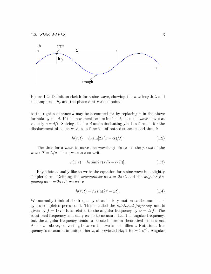
Figure 1.2: Definition sketch for a sine wave, showing the wavelength λ andthe amplitude h0 and the phase φ at various points.
to the right a distance d may be accounted for by replacing x in the aboveformula by x− d. If this movement occurs in time t, then the wave moves atvelocity c = d/t. Solving this for d and substituting yields a formula for thedisplacement of a sine wave as a function of both distance x and time t:
h(x, t) = h0 sin[2π(x− ct)/λ]. (1.2)
The time for a wave to move one wavelength is called the period of thewave: T = λ/c. Thus, we can also write
h(x, t) = h0 sin[2π(x/λ− t/T )]. (1.3)
Physicists actually like to write the equation for a sine wave in a slightlysimpler form. Defining the wavenumber as k = 2π/λ and the angular fre-
quency as ω = 2π/T , we write
h(x, t) = h0 sin(kx− ωt). (1.4)
We normally think of the frequency of oscillatory motion as the number ofcycles completed per second. This is called the rotational frequency, and isgiven by f = 1/T . It is related to the angular frequency by ω = 2πf . Therotational frequency is usually easier to measure than the angular frequency,but the angular frequency tends to be used more in theoretical discussions.As shown above, converting between the two is not difficult. Rotational fre-quency is measured in units of hertz, abbreviated Hz; 1 Hz = 1 s−1. Angular

4 CHAPTER 1. WAVES IN ONE DIMENSION
frequency also has the dimensions of inverse time, e. g., inverse seconds, butthe term “hertz” is generally reserved only for rotational frequency.
The argument of the sine function is by definition an angle. We refer tothis angle as the phase of the wave, φ = kx−ωt. The difference in the phaseof a wave at fixed time over a distance of one wavelength is 2π, as is thedifference in phase at fixed position over a time interval of one wave period.
Since angles are dimensionless, we normally don’t include this in the unitsfor frequency. However, it sometimes clarifies things to refer to the dimen-sions of rotational frequency as “rotations per second” or angular frequencyas “radians per second”.
As previously noted, we call h0, the maximum displacement of the wave,the amplitude. Often we are interested in the intensity of a wave, which isdefined as the square of the amplitude, I = h2
0.
The wave speed we have defined above, c = λ/T , is actually called thephase speed. Since λ = 2π/k and T = 2π/ω, we can write the phase speedin terms of the angular frequency and the wavenumber:
c =ω
k(phase speed). (1.5)
1.3 Types of Waves
In order to make the above material more concrete, we now examine thecharacteristics of various types of waves which may be observed in the realworld.
1.3.1 Ocean Surface Waves
These waves are manifested as undulations of the ocean surface as seen infigure 1.3. The speed of ocean waves is given by the formula
c =
(
g tanh(kH)
k
)1/2
, (1.6)
where g = 9.8 m s−2 is a constant related to the strength of the Earth’sgravity, H is the depth of the ocean, and the hyperbolic tangent is defined

1.3. TYPES OF WAVES 5
H
Figure 1.3: Wave on an ocean of depth H . The wave is moving to the rightand the particles of water at the surface move up and down as shown by thesmall vertical arrows.
as1
tanh(x) =exp(x) − exp(−x)
exp(x) + exp(−x). (1.7)
As figure 1.4 shows, for |x| ≪ 1, we can approximate the hyperbolictangent by tanh(x) ≈ x, while for |x| ≫ 1 it is +1 for x > 0 and −1 forx < 0. This leads to two limits: Since x = kH , the shallow water limit,which occurs when kH ≪ 1, yields a wave speed of
c ≈ (gH)1/2, (shallow water waves), (1.8)
while the deep water limit, which occurs when kH ≫ 1, yields
c ≈ (g/k)1/2, (deep water waves). (1.9)
Notice that the speed of shallow water waves depends only on the depthof the water and on g. In other words, all shallow water waves move atthe same speed. On the other hand, deep water waves of longer wavelength(and hence smaller wavenumber) move more rapidly than those with shorterwavelength. Waves for which the wave speed varies with wavelength arecalled dispersive. Thus, deep water waves are dispersive, while shallow waterwaves are non-dispersive.
For water waves with wavelengths of a few centimeters or less, surfacetension becomes important to the dynamics of the waves. In the deep water
1The notation exp(x) is just another way of writing the exponential function ex. We
prefer this way because it is prettier when the function argument is complicated.

6 CHAPTER 1. WAVES IN ONE DIMENSION
-1.00
-0.50
0.00
0.50
-4.00 -2.00 0.00 2.00tanh(x) vs x
Figure 1.4: Plot of the function tanh(x). The dashed line shows our approx-imation tanh(x) ≈ x for |x| ≪ 1.
case the wave speed at short wavelengths is actually given by the formula
c = (g/k + Ak)1/2 (1.10)
where the constant A is related to an effect called surface tension. For anair-water interface near room temperature, A ≈ 74 cm3 s−2.
1.3.2 Sound Waves
Sound is a longitudinal compression-expansion wave in a gas. The wavespeed is
c = (γRTabs)1/2 (1.11)
where γ and R are constants and Tabs is the absolute temperature. Theabsolute temperature is measured in Kelvins and is numerically given by
Tabs = TC + 273◦ (1.12)
where TC is the temperature in Celsius degrees. The angular frequency ofsound waves is thus given by
ω = ck = (γRTabs)1/2k. (1.13)
The speed of sound in air at normal temperatures is about 340 m s−1.

1.4. SUPERPOSITION PRINCIPLE 7
1.3.3 Light
Light moves in a vacuum at a speed of cvac = 3 × 10⁸ m s−1. In transparentmaterials it moves at a speed less than cvac by a factor n which is called therefractive index of the material:
c = cvac/n. (1.14)
Often the refractive index takes the form
n2 ≈ 1 +A
1 − (k/kR)2, (1.15)
where k is the wavenumber and kR and A are positive constants characteristicof the material. The angular frequency of light in a transparent medium isthus
ω = kc = kcvac/n. (1.16)
1.4 Superposition Principle
It is found empirically that as long as the amplitudes of waves in most mediaare small, two waves in the same physical location don’t interact with eachother. Thus, for example, two waves moving in the opposite direction simplypass through each other without their shapes or amplitudes being changed.When collocated, the total wave displacement is just the sum of the displace-ments of the individual waves. This is called the superposition principle. Atsufficiently large amplitude the superposition principle often breaks down —interacting waves may scatter off of each other, lose amplitude, or changetheir form.
Interference is a consequence of the superposition principle. When two ormore waves are superimposed, the net wave displacement is just the algebraicsum of the displacements of the individual waves. Since these displacementscan be positive or negative, the net displacement can either be greater or lessthan the individual wave displacements. The former case is called construc-
tive interference, while the latter is called destructive interference.Let us see what happens when we superimpose two sine waves with dif-
ferent wavenumbers. Figure 1.5 shows the superposition of two waves withwavenumbers k1 = 4 and k2 = 5. Notice that the result is a wave with aboutthe same wavelength as the two initial waves, but which varies in amplitude

8 CHAPTER 1. WAVES IN ONE DIMENSION
-1.00
-0.50
0.00
0.50
-10.0 -5.0 0.0 5.0sine functions vs x
-2.00
-1.00
0.00
1.00
-10.0 -5.0 0.0 5.0sum of functions vs x
k1, k2 = 4.000000 5.000000
Figure 1.5: Superposition (lower panel) of two sine waves (shown individuallyin the upper panel) with equal amplitudes and wavenumbers k1 = 4 andk2 = 5.
depending on whether the two sine waves are in or out of phase. When thewaves are in phase, constructive interference is occurring, while destructiveinterference occurs where the waves are out of phase.
What happens when the wavenumbers of the two sine waves are changed?Figure 1.6 shows the result when k1 = 10 and k2 = 11. Notice that thoughthe wavelength of the resultant wave is decreased, the locations where theamplitude is maximum have the same separation in x as in figure 1.5.
If we superimpose waves with k1 = 10 and k2 = 12, as is shown in figure1.7, we see that the x spacing of the regions of maximum amplitude hasdecreased by a factor of two. Thus, while the wavenumber of the resultantwave seems to be related to something like the average of the wavenumbersof the component waves, the spacing between regions of maximum waveamplitude appears to go inversely with the difference of the wavenumbers ofthe component waves. In other words, if k1 and k2 are close together, theamplitude maxima are far apart and vice versa.
We can symbolically represent the sine waves that make up figures 1.5,1.6, and 1.7 by a plot such as that shown in figure 1.8. The amplitudes andwavenumbers of each of the sine waves are indicated by vertical lines in this

1.4. SUPERPOSITION PRINCIPLE 9
-1.00
-0.50
0.00
0.50
-10.0 -5.0 0.0 5.0sine functions vs x
-2.00
-1.00
0.00
1.00
-10.0 -5.0 0.0 5.0sum of functions vs x
k1, k2 = 10.000000 11.000000
Figure 1.6: Superposition of two sine waves with equal amplitudes andwavenumbers k1 = 10 and k2 = 11.
-1.00
-0.50
0.00
0.50
-10.0 -5.0 0.0 5.0sine functions vs x
-2.00
-1.00
0.00
1.00
-10.0 -5.0 0.0 5.0sum of functions vs x
k1, k2 = 10.000000 12.000000
Figure 1.7: Superposition of two sine waves with equal amplitudes andwavenumbers k1 = 10 and k2 = 12.

10 CHAPTER 1. WAVES IN ONE DIMENSION
∆k ∆k
k 1 k 2
k 0
ampl
itude
wavenumber
2 waves
Figure 1.8: Representation of the wavenumbers and amplitudes of two su-perimposed sine waves.
figure.
The regions of large wave amplitude are called wave packets. Wave pack-ets will play a central role in what is to follow, so it is important that weacquire a good understanding of them. The wave packets produced by onlytwo sine waves are not well separated along the x-axis. However, if we super-impose many waves, we can produce an isolated wave packet. For example,figure 1.9 shows the results of superimposing 20 sine waves with wavenumbersk = 0.4m, m = 1, 2, . . . , 20, where the amplitudes of the waves are largestfor wavenumbers near k = 4. In particular, we assume that the amplitudeof each sine wave is proportional to exp[−(k − k0)
2/∆k2], where k0 = 4 and∆k = 1. The amplitudes of each of the sine waves making up the wave packetin figure 1.9 are shown schematically in figure 1.10.
The quantity ∆k controls the distribution of the sine waves being super-imposed — only those waves with a wavenumber k within approximately ∆kof the central wavenumber k0 of the wave packet, i. e., for 3 ≤ k ≤ 5 inthis case, contribute significantly to the sum. If ∆k is changed to 2, so thatwavenumbers in the range 2 ≤ k ≤ 6 contribute significantly, the wavepacketbecomes narrower, as is shown in figures 1.11 and 1.12. ∆k is called thewavenumber spread of the wave packet, and it evidently plays a role similarto the difference in wavenumbers in the superposition of two sine waves —the larger the wavenumber spread, the smaller the physical size of the wavepacket. Furthermore, the wavenumber of the oscillations within the wavepacket is given approximately by the central wavenumber.

1.4. SUPERPOSITION PRINCIPLE 11
-5.00
-2.50
0.00
2.50
-10.0 -5.0 0.0 5.0displacement vs x
k0 = 4.000000; dk = 1.000000; nwaves = 20
Figure 1.9: Superposition of twenty sine waves with k0 = 4 and ∆k = 1.
k 0
∆k
ampl
itude
0 4wavenumber8 12 16 20
Figure 1.10: Representation of the wavenumbers and amplitudes of 20 su-perimposed sine waves with k0 = 4 and ∆k = 1.

12 CHAPTER 1. WAVES IN ONE DIMENSION
-10.0
-5.0
0.0
5.0
-10.0 -5.0 0.0 5.0displacement vs x
k0 = 4.000000; dk = 2.000000; nwaves = 20
Figure 1.11: Superposition of twenty sine waves with k0 = 4 and ∆k = 2.
k 0
∆k
ampl
itude
0 4wavenumber8 12 16 20
Figure 1.12: Representation of the wavenumbers and amplitudes of 20 su-perimposed sine waves with k0 = 4 and ∆k = 2.
1.5. BEATS 13
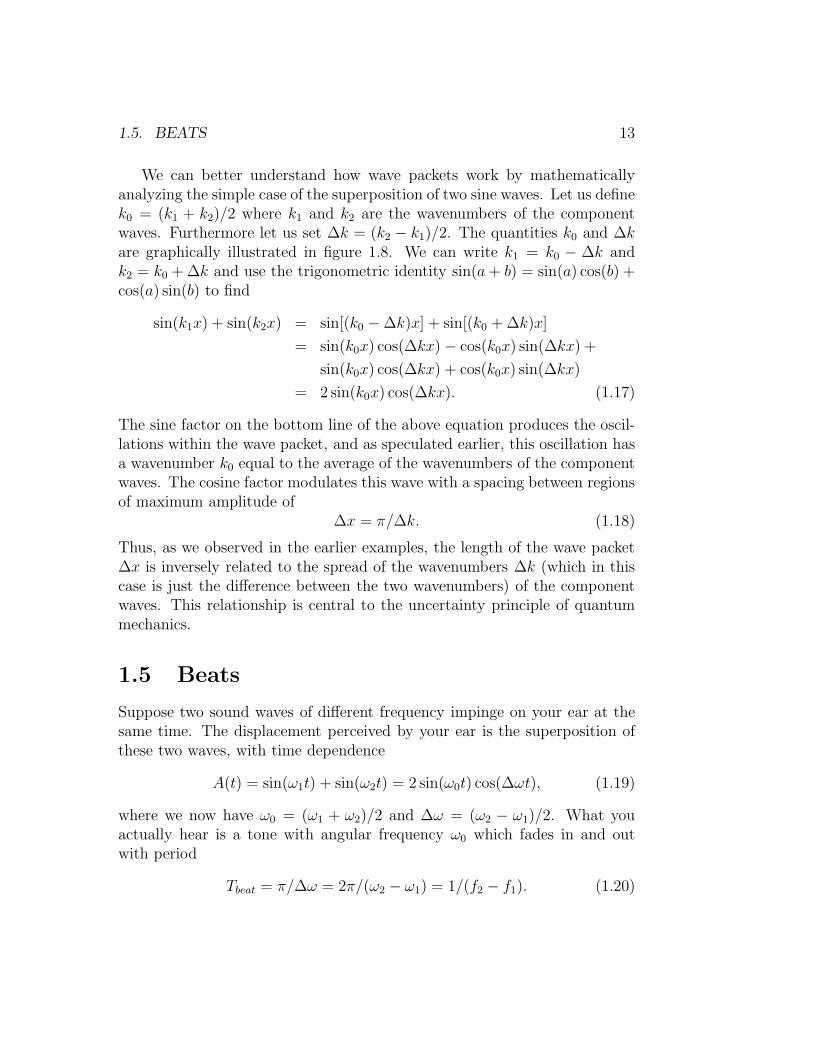
We can better understand how wave packets work by mathematicallyanalyzing the simple case of the superposition of two sine waves. Let us definek0 = (k1 + k2)/2 where k1 and k2 are the wavenumbers of the componentwaves. Furthermore let us set ∆k = (k2 − k1)/2. The quantities k0 and ∆kare graphically illustrated in figure 1.8. We can write k1 = k0 − ∆k andk2 = k0 + ∆k and use the trigonometric identity sin(a+ b) = sin(a) cos(b) +cos(a) sin(b) to find
sin(k1x) + sin(k2x) = sin[(k0 − ∆k)x] + sin[(k0 + ∆k)x]
= sin(k0x) cos(∆kx) − cos(k0x) sin(∆kx) +
sin(k0x) cos(∆kx) + cos(k0x) sin(∆kx)
= 2 sin(k0x) cos(∆kx). (1.17)
The sine factor on the bottom line of the above equation produces the oscil-lations within the wave packet, and as speculated earlier, this oscillation hasa wavenumber k0 equal to the average of the wavenumbers of the componentwaves. The cosine factor modulates this wave with a spacing between regionsof maximum amplitude of
∆x = π/∆k. (1.18)
Thus, as we observed in the earlier examples, the length of the wave packet∆x is inversely related to the spread of the wavenumbers ∆k (which in thiscase is just the difference between the two wavenumbers) of the componentwaves. This relationship is central to the uncertainty principle of quantummechanics.
1.5 Beats
Suppose two sound waves of different frequency impinge on your ear at thesame time. The displacement perceived by your ear is the superposition ofthese two waves, with time dependence
A(t) = sin(ω1t) + sin(ω2t) = 2 sin(ω0t) cos(∆ωt), (1.19)
where we now have ω0 = (ω1 + ω2)/2 and ∆ω = (ω2 − ω1)/2. What youactually hear is a tone with angular frequency ω0 which fades in and outwith period
Tbeat = π/∆ω = 2π/(ω2 − ω1) = 1/(f2 − f1). (1.20)

14 CHAPTER 1. WAVES IN ONE DIMENSION
The beat frequency is simply
fbeat = 1/Tbeat = f2 − f1. (1.21)
Note how beats are the time analog of wave packets — the mathematicsare the same except that frequency replaces wavenumber and time replacesspace.
1.6 Interferometers
An interferometer is a device which splits a beam of light into two sub-beams, shifts the phase of one sub-beam with respect to the other, andthen superimposes the sub-beams so that they interfere constructively ordestructively, depending on the magnitude of the phase shift between them.In this section we study the Michelson interferometer and interferometriceffects in thin films.
1.6.1 The Michelson Interferometer
The American physicist Albert Michelson invented the optical interferome-ter illustrated in figure 1.13. The incoming beam is split into two beams bythe half-silvered mirror. Each sub-beam reflects off of another mirror whichreturns it to the half-silvered mirror, where the two sub-beams recombine asshown. One of the reflecting mirrors is movable by a sensitive micrometerdevice, allowing the path length of the corresponding sub-beam, and hencethe phase relationship between the two sub-beams, to be altered. As figure1.13 shows, the difference in path length between the two sub-beams is 2xbecause the horizontal sub-beam traverses the path twice. Thus, construc-tive interference occurs when this path difference is an integral number ofwavelengths, i. e.,
2x = mλ, m = 0,±1,±2, . . . (Michelson interferometer) (1.22)
where λ is the wavelength of the light and m is an integer. Note that m isthe number of wavelengths that fits evenly into the distance 2x.

1.6. INTERFEROMETERS 15
d
d + x
Michelson interferometer
half-silvered mirror
movable mirror
fixed mirror
Figure 1.13: Sketch of a Michelson interferometer.
d
n > 1
A
n = 1
B
C
incident wave fronts
Figure 1.14: Plane light wave normally incident on a transparent thin filmof thickness d and index of refraction n > 1. Partial reflection occurs atthe front surface of the film, resulting in beam A, and at the rear surface,resulting in beam B. Much of the wave passes completely through the film,as with C.

16 CHAPTER 1. WAVES IN ONE DIMENSION
1.7 Thin Films
One of the most revealing examples of interference occurs when light interactswith a thin film of transparent material such as a soap bubble. Figure 1.14shows how a plane wave normally incident on the film is partially reflectedby the front and rear surfaces. The waves reflected off the front and rearsurfaces of the film interfere with each other. The interference can be eitherconstructive or destructive depending on the phase difference between thetwo reflected waves.
If the wavelength of the incoming wave is λ, one would naively expectconstructive interference to occur between the A and B beams if 2d were anintegral multiple of λ.
Two factors complicate this picture. First, the wavelength inside the filmis not λ, but λ/n, where n is the index of refraction of the film. Constructiveinterference would then occur if 2d = mλ/n. Second, it turns out thatan additional phase shift of half a wavelength occurs upon reflection whenthe wave is incident on material with a higher index of refraction than themedium in which the incident beam is immersed. This phase shift doesn’toccur when light is reflected from a region with lower index of refraction thanfelt by the incident beam. Thus beam B doesn’t acquire any additional phaseshift upon reflection. As a consequence, constructive interference actuallyoccurs when
2d = (m+ 1/2)λ/n, m = 0, 1, 2, . . . (constructive interference) (1.23)
while destructive interference results when
2d = mλ/n, m = 0, 1, 2, . . . (destructive interference). (1.24)
When we look at a soap bubble, we see bands of colors reflected back froma light source. What is the origin of these bands? Light from ordinary sourcesis generally a mixture of wavelengths ranging from roughly λ = 4.5×10⁻⁷ m(violet light) to λ = 6.5 × 10⁻⁷ m (red light). In between violet and redwe also have blue, green, and yellow light, in that order. Because of thedifferent wavelengths associated with different colors, it is clear that for amixed light source we will have some colors interfering constructively whileothers interfere destructively. Those undergoing constructive interferencewill be visible in reflection, while those undergoing destructive interferencewill not.

1.8. MATH TUTORIAL — DERIVATIVES 17
tangent tocurve at point A
∆y
∆y
x∆
x∆
x
y
slope = /
y = y(x)
A
B
Figure 1.15: Estimation of the derivative, which is the slope of the tangentline. When point B approaches point A, the slope of the line AB approachesthe slope of the tangent to the curve at point A.
Another factor enters as well. If the light is not normally incident onthe film, the difference in the distances traveled between beams reflected offof the front and rear faces of the film will not be just twice the thicknessof the film. To understand this case quantitatively, we need the conceptof refraction, which will be developed later in the context of geometricaloptics. However, it should be clear that different wavelengths will undergoconstructive interference for different angles of incidence of the incominglight. Different portions of the thin film will in general be viewed at differentangles, and will therefore exhibit different colors under reflection, resultingin the colorful patterns normally seen in soap bubbles.
1.8 Math Tutorial — Derivatives
This section provides a quick introduction to the idea of the derivative. Oftenwe are interested in the slope of a line tangent to a function y(x) at somevalue of x. This slope is called the derivative and is denoted dy/dx. Sincea tangent line to the function can be defined at any point x, the derivative

18 CHAPTER 1. WAVES IN ONE DIMENSION
itself is a function of x:
g(x) =dy(x)
dx. (1.25)
As figure 1.15 illustrates, the slope of the tangent line at some point onthe function may be approximated by the slope of a line connecting twopoints, A and B, set a finite distance apart on the curve:
dy
dx≈
∆y
∆x. (1.26)
As B is moved closer to A, the approximation becomes better. In the limitwhen B moves infinitely close to A, it is exact.
Derivatives of some common functions are now given. In each case a is aconstant.
dxa
dx= axa−1 (1.27)
d
dxexp(ax) = a exp(ax) (1.28)
d
dxlog(ax) =
1
x(1.29)
d
dxsin(ax) = a cos(ax) (1.30)
d
dxcos(ax) = −a sin(ax) (1.31)
daf(x)
dx= a
df(x)
dx(1.32)
d
dx[f(x) + g(x)] =
df(x)
dx+dg(x)
dx(1.33)
d
dxf(x)g(x) =
df(x)
dxg(x) + f(x)
dg(x)
dx(product rule) (1.34)
d
dxf(y) =
df
dy
dy
dx(chain rule) (1.35)
The product and chain rules are used to compute the derivatives of com-plex functions. For instance,
d
dx(sin(x) cos(x)) =
d sin(x)
dxcos(x) + sin(x)
d cos(x)
dx= cos2(x) − sin2(x)
andd
dxlog(sin(x)) =
1
sin(x)
d sin(x)
dx=
cos(x)
sin(x).

1.9. GROUP VELOCITY 19
1.9 Group Velocity
We now ask the following question: How fast do wave packets move? Sur-prisingly, we often find that wave packets move at a speed very different fromthe phase speed, c = ω/k, of the wave composing the wave packet.
We shall find that the speed of motion of wave packets, referred to as thegroup velocity, is given by
u =dω
dk
∣
∣
∣
∣
∣
k=k0
(group velocity). (1.36)
The derivative of ω(k) with respect to k is first computed and then evaluatedat k = k0, the central wavenumber of the wave packet of interest.
The relationship between the angular frequency and the wavenumber fora wave, ω = ω(k), depends on the type of wave being considered. Whateverthis relationship turns out to be in a particular case, it is called the dispersion
relation for the type of wave in question.
As an example of a group velocity calculation, suppose we want to find thevelocity of deep ocean wave packets for a central wavelength of λ0 = 60 m.This corresponds to a central wavenumber of k0 = 2π/λ0 ≈ 0.1 m−1. Thephase speed of deep ocean waves is c = (g/k)1/2. However, since c ≡ ω/k,we find the frequency of deep ocean waves to be ω = (gk)1/2. The groupvelocity is therefore u ≡ dω/dk = (g/k)1/2/2 = c/2. For the specified centralwavenumber, we find that u ≈ (9.8 m s−2/0.1 m−1)1/2/2 ≈ 5 m s−1. Bycontrast, the phase speed of deep ocean waves with this wavelength is c ≈10 m s−1.
Dispersive waves are waves in which the phase speed varies with wavenum-ber. It is easy to show that dispersive waves have unequal phase and groupvelocities, while these velocities are equal for non-dispersive waves.
1.9.1 Derivation of Group Velocity Formula
We now derive equation (1.36). It is easiest to do this for the simplestwave packets, namely those constructed out of the superposition of just twosine waves. We will proceed by adding two waves with full space and timedependence:
A = sin(k1x− ω1t) + sin(k2x− ω2t) (1.37)

20 CHAPTER 1. WAVES IN ONE DIMENSION
After algebraic and trigonometric manipulations familiar from earlier sec-tions, we find
A = 2 sin(k0x− ω0t) cos(∆kx− ∆ωt), (1.38)
where as before we have k0 = (k1+k2)/2, ω0 = (ω1+ω2)/2, ∆k = (k2−k1)/2,and ∆ω = (ω2−ω1)/2. Again think of this as a sine wave of frequency ω0 andwavenumber k0 modulated by a cosine function. In this case the modulationpattern moves with a speed so as to keep the argument of the cosine functionconstant:
∆kx− ∆ωt = const. (1.39)
Differentiating this with respect to t while holding ∆k and ∆ω constantyields
u ≡dx
dt=
∆ω
∆k. (1.40)
In the limit in which the deltas become very small, this reduces to the deriva-tive
u =dω
dk, (1.41)
which is the desired result.
1.9.2 Examples
We now illustrate some examples of phase speed and group velocity by show-ing the displacement resulting from the superposition of two sine waves, asgiven by equation (1.38), in the x-t plane. This is an example of a spacetimediagram, of which we will see many examples latter on.
Figure 1.16 shows a non-dispersive case in which the phase speed equalsthe group velocity. The regions with vertical and horizontal hatching (shortvertical or horizontal lines) indicate where the wave displacement is large andpositive or large and negative. Large displacements indicate the location ofwave packets. The positions of waves and wave packets at any given time maytherefore be determined by drawing a horizontal line across the graph at thedesired time and examining the variations in wave displacement along thisline. The crests of the waves are indicated by regions of short vertical lines.Notice that as time increases, the crests move to the right. This correspondsto the motion of the waves within the wave packets. Note also that the wavepackets, i. e., the broad regions of large positive and negative amplitudes,move to the right with increasing time as well.

1.9. GROUP VELOCITY 21
0.00
2.00
4.00
6.00
8.00
-10.0 -5.0 0.0 5.0time vs x
k_mean = 4.500000; delta_k = 0.500000
omega_mean = 4.500000; delta_omega = 0.500000
phase speed = 1.000000; group velocity = 1.000000
Figure 1.16: Net displacement of the sum of two traveling sine waves plottedin the x− t plane. The short vertical lines indicate where the displacement islarge and positive, while the short horizontal lines indicate where it is largeand negative. One wave has k = 4 and ω = 4, while the other has k = 5and ω = 5. Thus, ∆k = 5 − 4 = 1 and ∆ω = 5 − 4 = 1 and we haveu = ∆ω/∆k = 1. Notice that the phase speed for the first sine wave isc1 = 4/4 = 1 and for the second wave is c2 = 5/5 = 1. Thus, c1 = c2 = u inthis case.

22 CHAPTER 1. WAVES IN ONE DIMENSION
0.00
2.00
4.00
6.00
8.00
-10.0 -5.0 0.0 5.0time vs x
k_mean = 5.000000; delta_k = 0.500000
omega_mean = 5.000000; delta_omega = 1.000000
phase speed = 1.000000; group velocity = 2.000000
Figure 1.17: Net displacement of the sum of two traveling sine waves plottedin the x-t plane. One wave has k = 4.5 and ω = 4, while the other hask = 5.5 and ω = 6. In this case ∆k = 5.5−4.5 = 1 while ∆ω = 6−4 = 2, sothe group velocity is u = ∆ω/∆k = 2/1 = 2. However, the phase speeds forthe two waves are c1 = 4/4.5 = 0.889 and c2 = 6/5.5 = 1.091. The averageof the two phase speeds is about 0.989, so the group velocity is about twicethe average phase speed in this case.
Since velocity is distance moved ∆x divided by elapsed time ∆t, theslope of a line in figure 1.16, ∆t/∆x, is one over the velocity of whateverthat line represents. The slopes of lines representing crests (the slanted lines,not the short horizontal and vertical lines) are the same as the slopes oflines representing wave packets in this case, which indicates that the twomove at the same velocity. Since the speed of movement of wave crests isthe phase speed and the speed of movement of wave packets is the groupvelocity, the two velocities are equal and the non-dispersive nature of thiscase is confirmed.
Figure 1.17 shows a dispersive wave in which the group velocity is twicethe phase speed, while figure 1.18 shows a case in which the group velocity isactually opposite in sign to the phase speed. See if you can confirm that thephase and group velocities seen in each figure correspond to the values forthese quantities calculated from the specified frequencies and wavenumbers.

1.9. GROUP VELOCITY 23
0.00
2.00
4.00
6.00
8.00
-10.0 -5.0 0.0 5.0time vs x
k_mean = 4.500000; delta_k = 0.500000
omega_mean = 4.500000; delta_omega = -0.500000
phase speed = 1.000000; group velocity = -1.000000
Figure 1.18: Net displacement of the sum of two traveling sine waves plottedin the x-t plane. One wave has k = 4 and ω = 5, while the other has k = 5and ω = 4. Can you figure out the group velocity and the average phasespeed in this case? Do these velocities match the apparent phase and groupspeeds in the figure?

24 CHAPTER 1. WAVES IN ONE DIMENSION
1.10 Problems
1. Measure your pulse rate. Compute the ordinary frequency of your heartbeat in cycles per second. Compute the angular frequency in radiansper second. Compute the period.
2. An important wavelength for radio waves in radio astronomy is 21 cm.(This comes from neutral hydrogen.) Compute the wavenumber of thiswave. Compute the ordinary and angular frequencies. (The speed oflight is 3 × 10⁸ m s−1.)
3. Sketch the resultant wave obtained from superimposing the waves A =sin(2x) and B = sin(3x). By using the trigonometric identity given inequation (1.17), obtain a formula for A+ B in terms of sin(5x/2) andcos(x/2). Does the wave obtained from sketching this formula agreewith your earlier sketch?
4. Two sine waves with wavelengths λ1 and λ2 are superimposed, makingwave packets of length L. If we wish to make L larger, should we makeλ1 and λ2 closer together or farther apart? Explain your reasoning.
5. By examining figure 1.9 versus figure 1.10 and then figure 1.11 versusfigure 1.12, determine whether equation (1.18) works at least in anapproximate sense for isolated wave packets.
6. The frequencies of the chromatic scale in music are given by
fi = f02i/12, i = 0, 1, 2, . . . , 11, (1.42)
where f0 is a constant equal to the frequency of the lowest note in thescale.
(a) Compute f1 through f11 if f0 = 440 Hz (the “A” note).
(b) Using the above results, what is the beat frequency between the“A” (i = 0) and “B” (i = 2) notes? (The frequencies are givenhere in cycles per second rather than radians per second.)
(c) Which pair of the above frequencies f0 − f11 yields the smallestbeat frequency? Explain your reasoning.

1.10. PROBLEMS 25
microwavesource
microwavedetector
Figure 1.19: Sketch of a police radar.
7. Large ships in general cannot move faster than the phase speed ofsurface waves with a wavelength equal to twice the ship’s length. Thisis because most of the propulsive force goes into making big wavesunder these conditions rather than accelerating the ship.
(a) How fast can a 300 m long ship move in very deep water?
(b) As the ship moves into shallow water, does its maximum speedincrease or decrease? Explain.
8. Given the formula for refractive index of light quoted in this section, forwhat range of k does the phase speed of light in a transparent materialtake on real values which exceed the speed of light in a vacuum?
9. A police radar works by splitting a beam of microwaves, part of whichis reflected back to the radar from your car where it is made to interferewith the other part which travels a fixed path, as shown in figure 1.19.
(a) If the wavelength of the microwaves is λ, how far do you have totravel in your car for the interference between the two beams togo from constructive to destructive to constructive?
(b) If you are traveling toward the radar at speed v = 30 m s−1, usethe above result to determine the number of times per secondconstructive interference peaks will occur. Assume that λ = 3 cm.
10. Suppose you know the wavelength of light passing through a Michelsoninterferometer with high accuracy. Describe how you could use theinterferometer to measure the length of a small piece of material.

26 CHAPTER 1. WAVES IN ONE DIMENSION
partially reflecting surfacesd
Figure 1.20: Sketch of a Fabry-Perot interferometer.
11. A Fabry-Perot interferometer (see figure 1.20) consists of two parallelhalf-silvered mirrors placed a distance d from each other as shown. Thebeam passing straight through interferes with the beam which reflectsonce off of both of the mirrored surfaces as shown. For wavelength λ,what values of d result in constructive interference?
12. A Fabry-Perot interferometer has spacing d = 2 cm between the glassplates, causing the direct and doubly reflected beams to interfere (seefigure 1.20). As air is pumped out of the gap between the plates,the beams go through 23 cycles of constructive-destructive-constructiveinterference. If the wavelength of the light in the interfering beams is5× 10−7 m, determine the index of refraction of the air initially in theinterferometer.
13. Measurements on a certain kind of wave reveal that the angular fre-quency of the wave varies with wavenumber as shown in the followingtable:
ω (s−1) k (m−1)5 120 245 380 4125 5
(a) Compute the phase speed of the wave for k = 3 m−1 and fork = 4 m−1.
(b) Estimate the group velocity for k = 3.5 m−1 using a finite differ-ence approximation to the derivative.

1.10. PROBLEMS 27
A
B
D
k
ω
C E
Figure 1.21: Sketch of a weird dispersion relation.
14. Suppose some type of wave has the (admittedly weird) dispersion rela-tion shown in figure 1.21.
(a) For what values of k is the phase speed of the wave positive?
(b) For what values of k is the group velocity positive?
15. Compute the group velocity for shallow water waves. Compare it withthe phase speed of shallow water waves. (Hint: You first need to derivea formula for ω(k) from c(k).)
16. Repeat the above problem for deep water waves.
17. Repeat for sound waves. What does this case have in common withshallow water waves?

28 CHAPTER 1. WAVES IN ONE DIMENSION
Chapter 2
Waves in Two and Three
Dimensions
In this chapter we extend the ideas of the previous chapter to the case ofwaves in more than one dimension. The extension of the sine wave to higherdimensions is the plane wave. Wave packets in two and three dimensionsarise when plane waves moving in different directions are superimposed.
Diffraction results from the disruption of a wave which is impingent uponan object. Those parts of the wave front hitting the object are scattered,modified, or destroyed. The resulting diffraction pattern comes from thesubsequent interference of the various pieces of the modified wave. A knowl-edge of diffraction is necessary to understand the behavior and limitations ofoptical instruments such as telescopes.
Diffraction and interference in two and three dimensions can be manipu-lated to produce useful devices such as the diffraction grating.
2.1 Math Tutorial — Vectors
Before we can proceed further we need to explore the idea of a vector. Avector is a quantity which expresses both magnitude and direction. Graph-ically we represent a vector as an arrow. In typeset notation a vector isrepresented by a boldface character, while in handwriting an arrow is drawnover the character representing the vector.
Figure 2.1 shows some examples of displacement vectors, i. e., vectorswhich represent the displacement of one object from another, and introduces
29

30 CHAPTER 2. WAVES IN TWO AND THREE DIMENSIONS
A y
C y
B y
A x B xC x
xMary
A
BC
George
Pauly
Figure 2.1: Displacement vectors in a plane. Vector A represents the dis-placement of George from Mary, while vector B represents the displacementof Paul from George. Vector C represents the displacement of Paul fromMary and C = A + B. The quantities Ax, Ay, etc., represent the Cartesiancomponents of the vectors.
2.1. MATH TUTORIAL — VECTORS 31
x
y
θA
A = A cos
A = A sin y
x
θ
θ
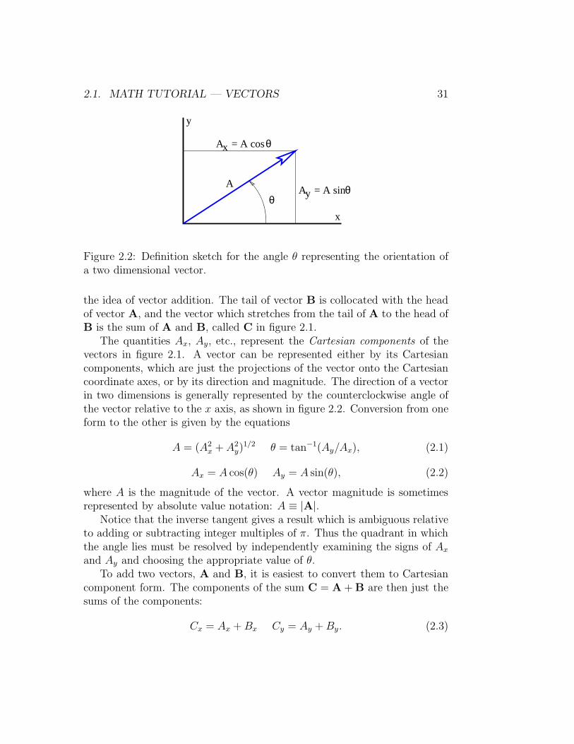
Figure 2.2: Definition sketch for the angle θ representing the orientation ofa two dimensional vector.
the idea of vector addition. The tail of vector B is collocated with the headof vector A, and the vector which stretches from the tail of A to the head ofB is the sum of A and B, called C in figure 2.1.
The quantities Ax, Ay, etc., represent the Cartesian components of thevectors in figure 2.1. A vector can be represented either by its Cartesiancomponents, which are just the projections of the vector onto the Cartesiancoordinate axes, or by its direction and magnitude. The direction of a vectorin two dimensions is generally represented by the counterclockwise angle ofthe vector relative to the x axis, as shown in figure 2.2. Conversion from oneform to the other is given by the equations
A = (A2
x + A2
y)1/2 θ = tan−1(Ay/Ax), (2.1)
Ax = A cos(θ) Ay = A sin(θ), (2.2)
where A is the magnitude of the vector. A vector magnitude is sometimesrepresented by absolute value notation: A ≡ |A|.
Notice that the inverse tangent gives a result which is ambiguous relativeto adding or subtracting integer multiples of π. Thus the quadrant in whichthe angle lies must be resolved by independently examining the signs of Ax
and Ay and choosing the appropriate value of θ.To add two vectors, A and B, it is easiest to convert them to Cartesian
component form. The components of the sum C = A + B are then just thesums of the components:
Cx = Ax +Bx Cy = Ay +By. (2.3)

32 CHAPTER 2. WAVES IN TWO AND THREE DIMENSIONS
AB
θ
Ax
y
x
Figure 2.3: Definition sketch for dot product.
Subtraction of vectors is done similarly, e. g., if A = C −B, then
Ax = Cx − Bx Ay = Cy − By. (2.4)
A unit vector is a vector of unit length. One can always construct aunit vector from an ordinary vector by dividing the vector by its length:n = A/|A|. This division operation is carried out by dividing each of thevector components by the number in the denominator. Alternatively, if thevector is expressed in terms of length and direction, the magnitude of thevector is divided by the denominator and the direction is unchanged.
Unit vectors can be used to define a Cartesian coordinate system. Conven-tionally, i, j, and k indicate the x, y, and z axes of such a system. Note that i,j, and k are mutually perpendicular. Any vector can be represented in termsof unit vectors and its Cartesian components: A = Axi+Ayj+Azk. An alter-nate way to represent a vector is as a list of components: A = (Ax, Ay, Az).We tend to use the latter representation since it is somewhat more economicalnotation.
There are two ways to multiply two vectors, yielding respectively whatare known as the dot product and the cross product. The cross product yieldsanother vector while the dot product yields a number. Here we will discussonly the dot product.
Given vectors A and B, the dot product of the two is defined as
A · B ≡ |A||B| cos θ, (2.5)
where θ is the angle between the two vectors. An alternate expression forthe dot product exists in terms of the Cartesian components of the vectors:
A ·B = AxBx + AyBy. (2.6)

2.1. MATH TUTORIAL — VECTORS 33
θ
x
x’
yy’
RY’
Y
X’
X
ab
Figure 2.4: Definition figure for rotated coordinate system. The vector R hascomponents X and Y in the unprimed coordinate system and componentsX ′ and Y ′ in the primed coordinate system.
It is easy to show that this is equivalent to the cosine form of the dot productwhen the x axis lies along one of the vectors, as in figure 2.3. Notice inparticular that Ax = |A| cos θ, while Bx = |B| and By = 0. Thus, A · B =|A| cos θ|B| in this case, which is identical to the form given in equation (2.5).
All that remains to be proven for equation (2.6) to hold in general is toshow that it yields the same answer regardless of how the Cartesian coor-dinate system is oriented relative to the vectors. To do this, we must showthat AxBx + AyBy = A′
xB′
x + A′
yB′
y, where the primes indicate componentsin a coordinate system rotated from the original coordinate system.
Figure 2.4 shows the vector R resolved in two coordinate systems rotatedwith respect to each other. From this figure it is clear that X ′ = a + b.Focusing on the shaded triangles, we see that a = X cos θ and b = Y sin θ.Thus, we find X ′ = X cos θ + Y sin θ. Similar reasoning shows that Y ′ =−X sin θ + Y cos θ. Substituting these and using the trigonometric identitycos2 θ + sin2 θ = 1 results in
A′
xB′
x + A′
yB′
y = (Ax cos θ + Ay sin θ)(Bx cos θ +By sin θ)
+ (−Ax sin θ + Ay cos θ)(−Bx sin θ +By cos θ)
= AxBx + AyBy (2.7)

34 CHAPTER 2. WAVES IN TWO AND THREE DIMENSIONS
wave fronts
λ|k|
wave vector
Figure 2.5: Definition sketch for a plane sine wave in two dimensions. Thewave fronts are constant phase surfaces separated by one wavelength. Thewave vector is normal to the wave fronts and its length is the wavenumber.
thus proving the complete equivalence of the two forms of the dot productas given by equations (2.5) and (2.6). (Multiply out the above expression toverify this.)
A numerical quantity which doesn’t depend on which coordinate systemis being used is called a scalar. The dot product of two vectors is a scalar.However, the components of a vector, taken individually, are not scalars,since the components change as the coordinate system changes. Since thelaws of physics cannot depend on the choice of coordinate system being used,we insist that physical laws be expressed in terms of scalars and vectors, butnot in terms of the components of vectors.
In three dimensions the cosine form of the dot product remains the same,while the component form is
A · B = AxBx + AyBy + AzBz. (2.8)

2.2. PLANE WAVES 35
2.2 Plane Waves
A plane wave in two or three dimensions is like a sine wave in one dimensionexcept that crests and troughs aren’t points, but form lines (2-D) or planes(3-D) perpendicular to the direction of wave propagation. Figure 2.5 showsa plane sine wave in two dimensions. The large arrow is a vector calledthe wave vector, which defines (1) the direction of wave propagation by itsorientation perpendicular to the wave fronts, and (2) the wavenumber by itslength. We can think of a wave front as a line along the crest of the wave.The equation for the displacement associated with a plane sine wave in threedimensions at some instant in time is
A(x, y, z) = sin(k · x) = sin(kxx+ kyy + kzz). (2.9)
Since wave fronts are lines or surfaces of constant phase, the equation defininga wave front is simply k · x = const.
In the two dimensional case we simply set kz = 0. Therefore, a wavefront,or line of constant phase φ in two dimensions is defined by the equation
k · x = kxx+ kyy = φ (two dimensions). (2.10)
This can be easily solved for y to obtain the slope and intercept of thewavefront in two dimensions.
As for one dimensional waves, the time evolution of the wave is obtainedby adding a term −ωt to the phase of the wave. In three dimensions thewave displacement as a function of both space and time is given by
A(x, y, z, t) = sin(kxx+ kyy + kzz − ωt). (2.11)
The frequency depends in general on all three components of the wave vector.The form of this function, ω = ω(kx, ky, kz), which as in the one dimensionalcase is called the dispersion relation, contains information about the physicalbehavior of the wave.
Some examples of dispersion relations for waves in two dimensions are asfollows:
• Light waves in a vacuum in two dimensions obey
ω = c(k2
x + k2
y)1/2 (light), (2.12)
where c is the speed of light in a vacuum.

36 CHAPTER 2. WAVES IN TWO AND THREE DIMENSIONS
• Deep water ocean waves in two dimensions obey
ω = g1/2(k2
x + k2
y)1/4 (ocean waves), (2.13)
where g is the strength of the Earth’s gravitational field as before.
• Certain kinds of atmospheric waves confined to a vertical x − z planecalled gravity waves (not to be confused with the gravitational wavesof general relativity)1 obey
ω =Nkx
kz
(gravity waves), (2.14)
where N is a constant with the dimensions of inverse time called theBrunt-Vaisala frequency.
Contour plots of these dispersion relations are plotted in the upper pan-els of figure 2.6. These plots are to be interpreted like topographic maps,where the lines represent contours of constant elevation. In the case of fig-ure 2.6, constant values of frequency are represented instead. For simplicity,the actual values of frequency are not labeled on the contour plots, but arerepresented in the graphs in the lower panels. This is possible because fre-quency depends only on wave vector magnitude (k2
x + k2y)
1/2 for the first twoexamples, and only on wave vector direction θ for the third.
2.3 Superposition of Plane Waves
We now study wave packets in two dimensions by asking what the super-position of two plane sine waves looks like. If the two waves have differentwavenumbers, but their wave vectors point in the same direction, the re-sults are identical to those presented in the previous chapter, except thatthe wave packets are indefinitely elongated without change in form in thedirection perpendicular to the wave vector. The wave packets produced inthis case march along in the direction of the wave vectors and thus appear toa stationary observer like a series of passing pulses with broad lateral extent.
1Gravity waves in the atmosphere are vertical or slantwise oscillations of air parcelsproduced by buoyancy forces which push parcels back toward their original elevation aftera vertical displacement.

2.3. SUPERPOSITION OF PLANE WAVES 37
(k + k )x y2 2 1/2
(k + k )x y2 2 1/2
k x k x
k z
k x
k y k y
θ
ωωω
θ
−π/2 π/2
Light waves (2−D) Deep ocean waves Gravity waves
Figure 2.6: Contour plots of the dispersion relations for three kinds of wavesin two dimensions. In the upper panels the curves show lines or contoursalong which the frequency ω takes on constant values. Contours ar drawnfor equally spaced values of ω. For light and ocean waves the frequencydepends only on the magnitude of the wave vector, whereas for gravity wavesit depends only on the wave vector’s direction, as defined by the angle θ inthe upper right panel. These dependences for each wave type are illustratedin the lower panels.

38 CHAPTER 2. WAVES IN TWO AND THREE DIMENSIONS
Superimposing two plane waves which have the same frequency resultsin a stationary wave packet through which the individual wave fronts pass.This wave packet is also elongated indefinitely in some direction, but thedirection of elongation depends on the dispersion relation for the waves beingconsidered. One can think of such wave packets as steady beams, whichguide the individual phase waves in some direction, but don’t themselveschange with time. By superimposing multiple plane waves, all with the samefrequency, one can actually produce a single stationary beam, just as onecan produce an isolated pulse by superimposing multiple waves with wavevectors pointing in the same direction.
2.3.1 Two Waves of Identical Wavelength
If the frequency of a wave depends on the magnitude of the wave vector,but not on its direction, the wave’s dispersion relation is called isotropic. Inthe isotropic case two waves have the same frequency only if the lengths oftheir wave vectors, and hence their wavelengths, are the same. The first twoexamples in figure 2.6 satisfy this condition. In this section we investigatethe beams produced by superimposing isotropic waves of the same frequency.
We superimpose two plane waves with wave vectors k1 = (−∆kx, ky)and k2 = (∆kx, ky). The lengths of the wave vectors in both cases arek1 = k2 = (∆k2
x + k2y)
1/2:
A = sin(−∆kxx+ kyy − ωt) + sin(∆kxx+ kyy − ωt). (2.15)
If ∆kx ≪ ky, then both waves are moving approximately in the y direction.An example of such waves would be two light waves with the same frequenciesmoving in slightly different directions.
Applying the trigonometric identity for the sine of the sum of two angles(as we have done previously), equation (2.15) can be reduced to
A = 2 sin(kyy − ωt) cos(∆kxx). (2.16)
This is in the form of a sine wave moving in the y direction with phase speedcphase = ω/ky and wavenumber ky, modulated in the x direction by a cosinefunction. The distance w between regions of destructive interference in the xdirection tells us the width of the resulting beams, and is given by ∆kxw = π,so that
w = π/∆kx. (2.17)

2.3. SUPERPOSITION OF PLANE WAVES 39
ky
kx∆
λ
2y
x
α
w
Figure 2.7: Wave fronts and wave vectors of two plane waves with the samewavelength but oriented in different directions. The vertical bands showregions of constructive interference where wave fronts coincide. The verticalregions in between the bars have destructive interference, and hence definethe lateral boundaries of the beams produced by the superposition. Thecomponents ∆kx and ky of one of the wave vectors are shown.
Thus, the smaller ∆kx, the greater is the beam diameter. This behavior isillustrated in figure 2.7.
Figure 2.8 shows an example of the beams produced by superposition oftwo plane waves of equal wavelength oriented as in figure 2.7. It is easy toshow that the transverse width of the resulting wave packet satisfies equation(2.17).
2.3.2 Two Waves of Differing Wavelength
In the third example of figure 2.6, the frequency of the wave depends onlyon the direction of the wave vector, independent of its magnitude, which isjust the reverse of the case for an isotropic dispersion relation. In this casedifferent plane waves with the same frequency have wave vectors which pointin the same direction, but have different lengths.
More generally, one might have waves for which the frequency dependson both the direction and magnitude of the wave vector. In this case, twodifferent plane waves with the same frequency would typically have wavevectors which differed both in direction and magnitude. Such an example is

40 CHAPTER 2. WAVES IN TWO AND THREE DIMENSIONS
0.0
10.0
20.0
30.0
-30.0 -20.0 -10.0 0.0 10.0 20.0y vs x
(k_x1, k_x2, k_y1, k_y2) = (-0.10, 0.10, 1.00, 1.00)
Figure 2.8: Example of beams produced by two plane waves with the samewavelength moving in different directions. The wave vectors of the two wavesare k = (±0.1, 1.0). Regions of positive displacement are illustrated byvertical hatching, while negative displacement has horizontal hatching.

2.3. SUPERPOSITION OF PLANE WAVES 41
1 2
k0
k1k2
k−∆k∆
y
xw
λ λ
Figure 2.9: Wave fronts and wave vectors (k1 and k2) of two plane waves withdifferent wavelengths oriented in different directions. The slanted bands showregions of constructive interference where wave fronts coincide. The slantedregions in between the bars have destructive interference, and as previously,define the lateral limits of the beams produced by the superposition. Thequantities k0 and ∆k are also shown.
illustrated in figures 2.9 and 2.10. We now investigate the superposition ofnon-isotropic waves with the same frequency.
Mathematically, we can represent the superposition of these two waves asa generalization of equation (2.15):
A = sin[−∆kxx+ (ky + ∆ky)y− ωt] + sin[∆kxx+ (ky −∆ky)y−ωt]. (2.18)
In this equation we have given the first wave vector a y component ky + ∆ky
while the second wave vector has ky − ∆ky. As a result, the first wavehas overall wavenumber k1 = [∆k2
x + (ky + ∆ky)2]1/2 while the second has
k2 = [∆k2x + (ky − ∆ky)
2]1/2, so that k1 6= k2. Using the usual trigonometricidentity, we write equation (2.18) as
A = 2 sin(kyy − ωt) cos(−∆kxx+ ∆kyy). (2.19)
To see what this equation implies, notice that constructive interference be-tween the two waves occurs when −∆kxx + ∆kyy = mπ, where m is aninteger. Solving this equation for y yields y = (∆kx/∆ky)x + mπ/∆ky,which corresponds to lines with slope ∆kx/∆ky. These lines turn out to
42 CHAPTER 2. WAVES IN TWO AND THREE DIMENSIONS
0.0
10.0
20.0
30.0
-30.0 -20.0 -10.0 0.0 10.0 20.0y vs x
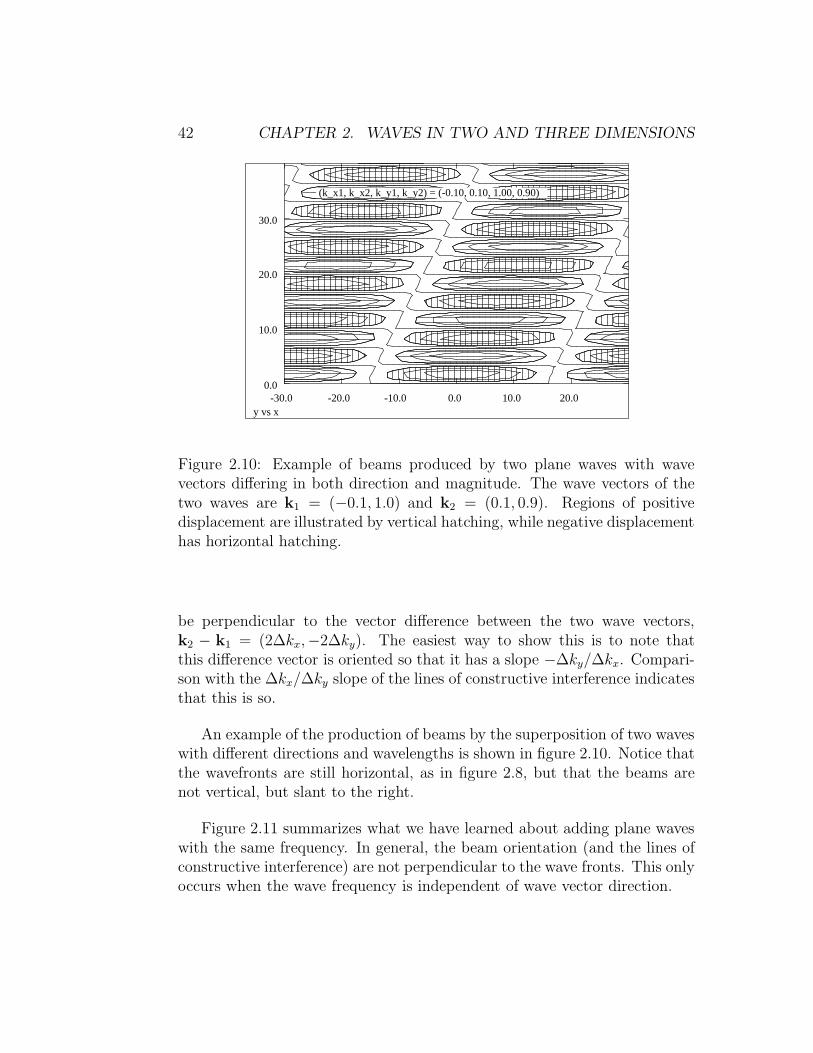
(k_x1, k_x2, k_y1, k_y2) = (-0.10, 0.10, 1.00, 0.90)
Figure 2.10: Example of beams produced by two plane waves with wavevectors differing in both direction and magnitude. The wave vectors of thetwo waves are k1 = (−0.1, 1.0) and k2 = (0.1, 0.9). Regions of positivedisplacement are illustrated by vertical hatching, while negative displacementhas horizontal hatching.
be perpendicular to the vector difference between the two wave vectors,k2 − k1 = (2∆kx,−2∆ky). The easiest way to show this is to note thatthis difference vector is oriented so that it has a slope −∆ky/∆kx. Compari-son with the ∆kx/∆ky slope of the lines of constructive interference indicatesthat this is so.
An example of the production of beams by the superposition of two waveswith different directions and wavelengths is shown in figure 2.10. Notice thatthe wavefronts are still horizontal, as in figure 2.8, but that the beams arenot vertical, but slant to the right.
Figure 2.11 summarizes what we have learned about adding plane waveswith the same frequency. In general, the beam orientation (and the lines ofconstructive interference) are not perpendicular to the wave fronts. This onlyoccurs when the wave frequency is independent of wave vector direction.

2.3. SUPERPOSITION OF PLANE WAVES 43
orientation ofbeam
orientation ofwave fronts
∆k−
∆k
ky
kx
k1
k2
k0
const.frequencycurve
Figure 2.11: Illustration of factors entering the addition of two plane waveswith the same frequency. The wave fronts are perpendicular to the vector av-erage of the two wave vectors, k0 = (k1+k2)/2, while the lines of constructiveinterference, which define the beam orientation, are oriented perpendicularto the difference between these two vectors, k2 − k1.
44 CHAPTER 2. WAVES IN TWO AND THREE DIMENSIONS
y
kx
k α
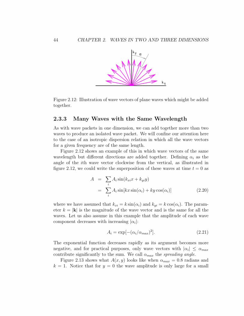
Figure 2.12: Illustration of wave vectors of plane waves which might be addedtogether.
2.3.3 Many Waves with the Same Wavelength
As with wave packets in one dimension, we can add together more than twowaves to produce an isolated wave packet. We will confine our attention hereto the case of an isotropic dispersion relation in which all the wave vectorsfor a given frequency are of the same length.
Figure 2.12 shows an example of this in which wave vectors of the samewavelength but different directions are added together. Defining αi as theangle of the ith wave vector clockwise from the vertical, as illustrated infigure 2.12, we could write the superposition of these waves at time t = 0 as
A =∑
i
Ai sin(kxix+ kyiy)
=∑
i
Ai sin[kx sin(αi) + ky cos(αi)] (2.20)
where we have assumed that kxi = k sin(αi) and kyi = k cos(αi). The param-eter k = |k| is the magnitude of the wave vector and is the same for all thewaves. Let us also assume in this example that the amplitude of each wavecomponent decreases with increasing |αi|:
Ai = exp[−(αi/αmax)2]. (2.21)
The exponential function decreases rapidly as its argument becomes morenegative, and for practical purposes, only wave vectors with |αi| ≤ αmax
contribute significantly to the sum. We call αmax the spreading angle.Figure 2.13 shows what A(x, y) looks like when αmax = 0.8 radians and
k = 1. Notice that for y = 0 the wave amplitude is only large for a small

2.3. SUPERPOSITION OF PLANE WAVES 45
0.0
10.0
20.0
30.0
-30.0 -20.0 -10.0 0.0 10.0 20.0y vs x
Half-angle of diffraction = 0.800000
Wavenumber = 1
Figure 2.13: Plot of the displacement field A(x, y) from equation (2.20) forαmax = 0.8 and k = 1.
0.0
10.0
20.0
30.0
-30.0 -20.0 -10.0 0.0 10.0 20.0y vs x
Half-angle of diffraction = 0.200000
Wavenumber = 1
Figure 2.14: Plot of the displacement field A(x, y) from equation (2.20) forαmax = 0.2 and k = 1.

46 CHAPTER 2. WAVES IN TWO AND THREE DIMENSIONS
region in the range −4 < x < 4. However, for y > 0 the wave spreads into abroad semicircular pattern.
Figure 2.14 shows the computed pattern of A(x, y) when the spreadingangle αmax = 0.2 radians. The wave amplitude is large for a much broaderrange of x at y = 0 in this case, roughly −12 < x < 12. On the other hand,the subsequent spread of the wave is much smaller than in the case of figure2.13.
We conclude that a superposition of plane waves with wave vectors spreadnarrowly about a central wave vector which points in the y direction (as infigure 2.14) produces a beam which is initially broad in x but for which thebreadth increases only slightly with increasing y. However, a superpositionof plane waves with wave vectors spread more broadly (as in figure 2.13)produces a beam which is initially narrow in x but which rapidly increasesin width as y increases.
The relationship between the spreading angle αmax and the initial breadthof the beam is made more understandable by comparison with the results forthe two-wave superposition discussed at the beginning of this section. Asindicated by equation (2.17), large values of kx, and hence α, are associatedwith small wave packet dimensions in the x direction and vice versa. Thesuperposition of two waves doesn’t capture the subsequent spread of thebeam which occurs when many waves are superimposed, but it does lead toa rough quantitative relationship between αmax (which is just tan−1(kx/ky) inthe two wave case) and the initial breadth of the beam. If we invoke the smallangle approximation for α = αmax so that αmax = tan−1(kx/ky) ≈ kx/ky ≈kx/k, then kx ≈ kαmax and equation (2.17) can be written w = π/kx ≈π/(kαmax) = λ/(2αmax). Thus, we can find the approximate spreading anglefrom the wavelength of the wave λ and the initial breadth of the beam w:
αmax ≈ λ/(2w) (single slit spreading angle). (2.22)
2.4 Diffraction Through a Single Slit
How does all of this apply to the passage of waves through a slit? Imagine aplane wave of wavelength λ impingent on a barrier with a slit. The barriertransforms the plane wave with infinite extent in the lateral direction into abeam with initial transverse dimensions equal to the width of the slit. Thesubsequent development of the beam is illustrated in figures 2.13 and 2.14,

2.5. TWO SLITS 47
narrow slitbroad spreading
broad slitnarrow spreading
Figure 2.15: Schematic behavior when a plane wave impinges on a narrowslit and a broad slit.
and schematically in figure 2.15. In particular, if the slit width is comparableto the wavelength, the beam spreads broadly as in figure 2.13. If the slit widthis large compared to the wavelength, the beam doesn’t spread as much, asfigure 2.14 illustrates. Equation (2.22) gives us an approximate quantitativeresult for the spreading angle if w is interpreted as the width of the slit.
One use of the above equation is in determining the maximum angu-lar resolution of optical instruments such as telescopes. The primary lensor mirror can be thought of as a rather large “slit”. Light from a distantpoint source is essentially in the form of a plane wave when it arrives at thetelescope. However, the light passed by the telescope is no longer a planewave, but is a beam with a tendency to spread. The spreading angle αmax
is given by equation (2.22), and the telescope cannot resolve objects withan angular separation less than αmax. Replacing w with the diameter of thelens or mirror in equation (2.22) thus yields the telescope’s angular resolu-tion. For instance, a moderate sized telescope with aperture 1 m observingred light with λ ≈ 6 × 10⁻⁷ m has a maximum angular resolution of about3 × 10−7 radians.

48 CHAPTER 2. WAVES IN TWO AND THREE DIMENSIONS
slit A
slit B
���������������������������
���������������������������
L 1
L 2
L 0
d sin θ
d
L θ
z
incidentwave front
m = −1
m = +1
m = 0
m = +1.5
m = +0.5
m = −0.5
m = −1.5
Figure 2.16: Definition sketch for the double slit. Light passing through slitB travels an extra distance to the screen equal to d sin θ compared to lightpassing through slit A.
2.5 Two Slits
Let us now imagine a plane sine wave normally impingent on a screen withtwo narrow slits spaced by a distance d, as shown in figure 2.16. Since theslits are narrow relative to the wavelength of the wave impingent on them,the spreading angle of the beams is large and the diffraction pattern fromeach slit individually is a cylindrical wave spreading out in all directions, asillustrated in figure 2.13. The cylindrical waves from the two slits interfere,resulting in oscillations in wave intensity at the screen on the right side offigure 2.16.
Constructive interference occurs when the difference in the paths traveledby the two waves from their originating slits to the screen, L2 − L1, is aninteger multiple m of the wavelength λ: L2 − L1 = mλ. If L0 ≫ d, the linesL1 and L2 are nearly parallel, which means that the narrow end of the darktriangle in figure 2.16 has an opening angle of θ. Thus, the path differencebetween the beams from the two slits is L2−L1 = d sin θ. Substitution of thisinto the above equation shows that constructive interference occurs when
d sin θ = mλ, m = 0,±1,±2, . . . (two slit interference). (2.23)
Destructive interference occurs when m is an integer plus 1/2. The integer

2.6. DIFFRACTION GRATINGS 49
-1.00
-0.50
0.00
0.50
-20.0 -10.0 0.0 10.0amplitude vs d*k*sin(theta)
0.00
0.25
0.50
0.75
-20.0 -10.0 0.0 10.0intensity vs d*k*sin(theta)
Number of grating lines = 2Wave packet envelope
Intensity
Figure 2.17: Amplitude and intensity of interference pattern from a diffrac-tion grating with 2 slits.
m is called the interference order and is the number of wavelengths by whichthe two paths differ.
2.6 Diffraction Gratings
Since the angular spacing ∆θ of interference peaks in the two slit case dependson the wavelength of the incident wave, the two slit system can be used as acrude device to distinguish between the wavelengths of different componentsof a non-sinusoidal wave impingent on the slits. However, if more slits areadded, maintaining a uniform spacing d between slits, we obtain a moresophisticated device for distinguishing beam components. This is called adiffraction grating.
Figures 2.17-2.19 show the amplitude and intensity of the diffraction pat-tern for gratings with 2, 4, and 16 slits respectively. Notice how the interfer-ence peaks remain in the same place but increase in sharpness as the numberof slits increases.
The width of the peaks is actually related to the overall width of thegrating, w = nd, where n is the number of slits. Thinking of this width asthe dimension of large single slit, the single slit equation, αmax = λ/(2w),

50 CHAPTER 2. WAVES IN TWO AND THREE DIMENSIONS
-2.00
-1.00
0.00
1.00
-20.0 -10.0 0.0 10.0amplitude vs d*k*sin(theta)
0.00
1.00
2.00
3.00
-20.0 -10.0 0.0 10.0intensity vs d*k*sin(theta)
Number of grating lines = 4Wave packet envelope
Intensity
Figure 2.18: Amplitude and intensity of interference pattern from a diffrac-tion grating with 4 slits.
-8.00
-4.00
0.00
4.00
-20.0 -10.0 0.0 10.0amplitude vs d*k*sin(theta)
0.0
16.0
32.0
48.0
-20.0 -10.0 0.0 10.0intensity vs d*k*sin(theta)
Number of grating lines = 16Wave packet envelope
Intensity
Figure 2.19: Amplitude and intensity of interference pattern from a diffrac-tion grating with 16 slits.

2.7. PROBLEMS 51
tells us the angular width of the peaks.Whereas the angular width of the interference peaks is governed by the
single slit equation, their angular positions are governed by the two slit equa-tion. Let us assume for simplicity that |θ| ≪ 1 so that we can make the smallangle approximation to the two slit equation, mλ = d sin θ ≈ dθ, and askthe following question: How different do two wavelengths have to be in orderthat the interference peaks from the two waves not overlap? In order forthe peaks to be distinguishable, they should be separated in θ by an angle∆θ = m∆λ/d, which is greater than the angular width of each peak, αmax:
∆θ > αmax. (2.24)
Substituting in the above expressions for ∆θ and αmax and solving for ∆λ, weget ∆λ > λ/(2mn), where n = w/d is the number of slits in the diffractiongrating. Thus, the fractional difference between wavelengths which can bedistinguished by a diffraction grating depends solely on the interference orderm and the number of slits n in the grating:
∆λ
λ>
1
2mn. (2.25)
2.7 Problems
1. Point A is at the origin. Point B is 3 m distant from A at 30◦ coun-terclockwise from the x axis. Point C is 2 m from point A at 100◦
counterclockwise from the x axis.
(a) Obtain the Cartesian components of the vector D1 which goesfrom A to B and the vector D2 which goes from A to C.
(b) Find the Cartesian components of the vector D3 which goes fromB to C.
(c) Find the direction and magnitude of D3.
2. For the vectors in the previous problem, find D1 · D2 using both thecosine form of the dot product and the Cartesian form. Check to seeif the two answers are the same.
3. Show graphically or otherwise that |A + B| 6= |A| + |B| except whenthe vectors A and B are parallel.

52 CHAPTER 2. WAVES IN TWO AND THREE DIMENSIONS
/4π
λ
y
x
k
Figure 2.20: Sketch of wave moving at 45◦ to the x-axis.
4. A wave in the x-y plane is defined by h = h0 sin(k · x) where k =(1, 2) cm−1.
(a) On a piece of graph paper draw x and y axes and then plot a linepassing through the origin which is parallel to the vector k.
(b) On the same graph plot the line defined by k · x = kxx + kyy =0, k · x = π, and k · x = 2π. Check to see if these lines areperpendicular to k.
5. A plane wave in two dimensions in the x−y plane moves in the direction45◦ counterclockwise from the x-axis as shown in figure 2.20. Determinehow fast the intersection between a wavefront and the x-axis movesto the right in terms of the phase speed c and wavelength λ of thewave. Hint: What is the distance between wavefronts along the x-axiscompared to the wavelength?
6. Two deep plane ocean waves with the same frequency ω are movingapproximately to the east. However, one wave is oriented a small angleβ north of east and the other is oriented β south of east.
(a) Determine the orientation of lines of constructive interference be-tween these two waves.
(b) Determine the spacing between lines of constructive interference.

2.7. PROBLEMS 53
ky
k x
kckb
ka
ω = 4
ω = 8
ω = 12
1 2-1
1
-1
Figure 2.21: Graphical representation of the dispersion relation for shallowwater waves in a river flowing in the x direction. Units of frequency are hertz,units of wavenumber are inverse meters.
7. An example of waves with a dispersion relation in which the frequencyis a function of both wave vector magnitude and direction is showngraphically in figure 2.21.
(a) What is the phase speed of the waves for each of the three wavevectors? Hint: You may wish to obtain the length of each wavevector graphically.
(b) For each of the wave vectors, what is the orientation of the wavefronts?
(c) For each of the illustrated wave vectors, sketch two other wave vec-tors whose average value is approximately the illustrated vector,and whose tips lie on the same frequency contour line. Deter-mine the orientation of lines of constructive interference producedby the superimposing pairs of plane waves for which each of thevector pairs are the wave vectors.
8. Two gravity waves have the same frequency, but slightly different wave-

54 CHAPTER 2. WAVES IN TWO AND THREE DIMENSIONS
lengths.
(a) If one wave has an orientation angle θ = π/4 radians, what is theorientation angle of the other? (See figure 2.6.)
(b) Determine the orientation of lines of constructive interference be-tween these two waves.
9. A plane wave impinges on a single slit, spreading out a half-angle αafter the slit. If the whole apparatus is submerged in a liquid withindex of refraction n = 1.5, how does the spreading angle of the lightchange? (Hint: Recall that the index of refraction in a transparentmedium is the ratio of the speed of light in a vacuum to the speedin the medium. Furthermore, when light goes from a vacuum to atransparent medium, the light frequency doesn’t change. Therefore,how does the wavelength of the light change?)
10. Determine the diameter of the telescope needed to resolve a planet2× 108 km from a star which is 6 light years from the earth. (Assumeblue light which has a wavelength λ ≈ 4 × 10⁻⁷ m = 400 nm. Also,don’t worry about the great difference in brightness between the twofor the purposes of this problem.)
11. A laser beam from a laser on the earth is bounced back to the earthby a corner reflector on the moon.
(a) Engineers find that the returned signal is stronger if the laser beamis initially spread out by the beam expander shown in figure 2.22.Explain why this is so.
(b) The beam has a diameter of 1 m leaving the earth. How broad isit when it reaches the moon, which is 4 × 10⁵ km away? Assumethe wavelength of the light to be 5 × 10⁻⁷ m.
(c) How broad would the laser beam be at the moon if it weren’tinitially passed through the beam expander? Assume its initialdiameter to be 1 cm.
12. Suppose that a plane wave hits two slits in a barrier at an angle, suchthat the phase of the wave at one slit lags the phase at the other slit byhalf a wavelength. How does the resulting interference pattern changefrom the case in which there is no lag?

2.7. PROBLEMS 55
1 m
laserbeam spreader
Figure 2.22: Sketch of a beam expander for a laser.
13. Suppose that a thin piece of glass of index of refraction n = 1.33 isplaced in front of one slit of a two slit diffraction setup.
(a) How thick does the glass have to be to slow down the incomingwave so that it lags the wave going through the other slit by aphase difference of π? Take the wavelength of the light to beλ = 6 × 10⁻⁷ m.
(b) For the above situation, describe qualitatively how the diffractionpattern changes from the case in which there is no glass in frontof one of the slits. Explain your results.
14. A light source produces two wavelengths, λ1 = 400 nm (blue) andλ2 = 600 nm (red).
(a) Qualitatively sketch the two slit diffraction pattern from this source.Sketch the pattern for each wavelength separately.
(b) Qualitatively sketch the 16 slit diffraction pattern from this source,where the slit spacing is the same as in the two slit case.
15. A light source produces two wavelengths, λ1 = 631 nm and λ2 =635 nm. What is the minimum number of slits needed in a gratingspectrometer to resolve the two wavelengths? (Assume that you arelooking at the first order diffraction peak.) Sketch the diffraction peakfrom each wavelength and indicate how narrow the peaks must be toresolve them.
56 CHAPTER 2. WAVES IN TWO AND THREE DIMENSIONS

Chapter 3
Geometrical Optics
As was shown previously, when a plane wave is impingent on an aperturewhich has dimensions much greater than the wavelength of the wave, diffrac-tion effects are minimal and a segment of the plane wave passes through theaperture essentially unaltered. This plane wave segment can be thought ofas a wave packet, called a beam or ray, consisting of a superposition of wavevectors very close in direction and magnitude to the central wave vector ofthe wave packet. In most cases the ray simply moves in the direction de-fined by the central wave vector, i. e., normal to the orientation of the wavefronts. However, this is not true when the medium through which the lightpropagates is optically anisotropic, i. e., light traveling in different directionsmoves at different phase speeds. An example of such a medium is a calcitecrystal. In the anisotropic case, the orientation of the ray can be determinedonce the dispersion relation for the waves in question is known, by using thetechniques developed in the previous chapter.
If light moves through some apparatus in which all apertures are muchgreater in dimension than the wavelength of light, then we can use the aboverule to follow rays of light through the apparatus. This is called the geomet-
rical optics approximation.
3.1 Reflection and Refraction
Most of what we need to know about geometrical optics can be summarizedin two rules, the laws of reflection and refraction. These rules may both beinferred by considering what happens when a plane wave segment impinges on
57

58 CHAPTER 3. GEOMETRICAL OPTICS
mirror
θR
θI
Figure 3.1: Sketch showing the reflection of a wave from a plane mirror. Thelaw of reflection states that θI = θR.
a flat surface. If the surface is polished metal, the wave is reflected, whereasif the surface is an interface between two transparent media with differingindices of refraction, the wave is partially reflected and partially refracted.Reflection means that the wave is turned back into the half-space from whichit came, while refraction means that it passes through the interface, acquiringa different direction of motion from that which it had before reaching theinterface.
Figure 3.1 shows the wave vector and wave front of a wave being reflectedfrom a plane mirror. The angles of incidence, θI , and reflection, θR, aredefined to be the angles between the incoming and outgoing wave vectorsrespectively and the line normal to the mirror. The law of reflection statesthat θR = θI . This is a consequence of the need for the incoming and outgoingwave fronts to be in phase with each other all along the mirror surface. Thisplus the equality of the incoming and outgoing wavelengths is sufficient toinsure the above result.
Refraction, as illustrated in figure 3.2, is slightly more complicated. SincenR > nI , the speed of light in the right-hand medium is less than in the left-hand medium. (Recall that the speed of light in a medium with refractiveindex n is cmedium = cvac/n.) The frequency of the wave packet doesn’tchange as it passes through the interface, so the wavelength of the light on

3.1. REFLECTION AND REFRACTION 59
A
B D
C
θI
θ R
n = n n = nI R
Figure 3.2: Sketch showing the refraction of a wave from an interface betweentwo dielectric media with n2 > n1.
the right side is less than the wavelength on the left side.
Let us examine the triangle ABC in figure 3.2. The side AC is equal tothe side BC times sin(θI). However, AC is also equal to 2λI , or twice thewavelength of the wave to the left of the interface. Similar reasoning showsthat 2λR, twice the wavelength to the right of the interface, equals BC timessin(θR). Since the interval BC is common to both triangles, we easily seethat
λI
λR=
sin(θI)
sin(θR). (3.1)
Since λI = cIT = cvacT/nI and λR = cRT = cvacT/nR where cI and cR arethe wave speeds to the left and right of the interface, cvac is the speed of lightin a vacuum, and T is the (common) period, we can easily recast the aboveequation in the form
nI sin(θI) = nR sin(θR). (3.2)
This is called Snell’s law, and it governs how a ray of light bends as it passesthrough a discontinuity in the index of refraction. The angle θI is called theincident angle and θR is called the refracted angle. Notice that these anglesare measured from the normal to the surface, not the tangent.

60 CHAPTER 3. GEOMETRICAL OPTICS
3.2 Total Internal Reflection
When light passes from a medium of lesser index of refraction to one withgreater index of refraction, Snell’s law indicates that the ray bends toward
the normal to the interface. The reverse occurs when the passage is in theother direction. In this latter circumstance a special situation arises whenSnell’s law predicts a value for the sine of the refracted angle greater thanone. This is physically untenable. What actually happens is that the incidentwave is reflected from the interface. This phenomenon is called total internal
reflection. The minimum incident angle for which total internal reflectionoccurs is obtained by substituting θR = π/2 into equation (3.2), resulting in
sin(θI) = nR/nI (total internal reflection). (3.3)
3.3 Anisotropic Media
Notice that Snell’s law makes the implicit assumption that rays of light movein the direction of the light’s wave vector, i. e., normal to the wave fronts.As the analysis in the previous chapter makes clear, this is valid only whenthe optical medium is isotropic, i. e., the wave frequency depends only onthe magnitude of the wave vector, not on its direction.
Certain kinds of crystals, such as those made of calcite, are not isotropic— the speed of light in such crystals, and hence the wave frequency, dependson the orientation of the wave vector. As an example, the angular frequencyin an isotropic medium might take the form
ω =
[
c21(kx + ky)
2
2+c22(kx − ky)
2
2
]1/2
, (3.4)
where c1 is the speed of light for waves in which ky = kx, and c2 is its speedwhen ky = −kx.
Figure 3.3 shows an example in which a ray hits a calcite crystal orientedso that constant frequency contours are as specified in equation (3.4). Thewave vector is oriented normal to the surface of the crystal, so that wavefronts are parallel to this surface. Upon entering the crystal, the wave frontorientation must stay the same to preserve phase continuity at the surface.However, due to the anisotropy of the dispersion relation for light in the

3.4. THIN LENS FORMULA AND OPTICAL INSTRUMENTS 61
ω = const.
direction ofray
k
Dispersion relation for crystal
crystal
k x
ky
Figure 3.3: The right panel shows the fate of a light ray normally incident onthe face of a properly cut calcite crystal. The anisotropic dispersion relationwhich gives rise to this behavior is shown in the left panel.
crystal, the ray direction changes as shown in the right panel. This behavioris clearly inconsistent with the usual version of Snell’s law!
It is possible to extend Snell’s law to the anisotropic case. However, wewill not present this here. The following discussions of optical instrumentswill always assume that isotropic optical media are used.
3.4 Thin Lens Formula and Optical Instru-
ments
Given the laws of reflection and refraction, one can see in principle how thepassage of light through an optical instrument could be traced. For each ofa number of initial rays, the change in the direction of the ray at each mirrorsurface or refractive index interface can be calculated. Between these points,the ray traces out a straight line.
Though simple in conception, this procedure can be quite complex inpractice. However, the procedure simplifies if a number of approximations,collectively called the thin lens approximation, are valid. We begin with thecalculation of the bending of a ray of light as it passes through a prism, asillustrated in figure 3.4.
The pieces of information needed to find θ, the angle through which the

62 CHAPTER 3. GEOMETRICAL OPTICS
α
θθ
θ
θ θ
3
4
21
Figure 3.4: Bending of a ray of light as it passes through a prism.
ray is deflected are as follows: The geometry of the triangle defined by theentry and exit points of the ray and the upper vertex of the prism leads to
α+ (π/2 − θ2) + (π/2 − θ3) = π, (3.5)
which simplifies toα = θ2 + θ3. (3.6)
Snell’s law at the entrance and exit points of the ray tell us that
n =sin(θ1)
sin(θ2)n =
sin(θ4)
sin(θ3), (3.7)
where n is the index of refraction of the prism. (The index of refraction ofthe surroundings is assumed to be unity.) One can also infer that
θ = θ1 + θ4 − α. (3.8)
This comes from the fact that the the sum of the internal angles of the shadedquadrangle in figure 3.4 is (π/2 − θ1) + α + (π/2 − θ4) + (π + θ) = 2π.
Combining equations (3.6), (3.7), and (3.8) allows the ray deflection θto be determined in terms of θ1 and α, but the resulting expression is verymessy. However, great simplification occurs if the following conditions aremet:
• The angle α≪ 1.
• The angles θ1 ≪ 1 and θ4 ≪ 1.

3.4. THIN LENS FORMULA AND OPTICAL INSTRUMENTS 63
θ
α
d do i
o ir
Figure 3.5: Light ray undergoing deflection through an angle θ by a lens.The angle α is the angle between the tangents to the entry and exit pointsof the ray on the lens.
With these approximations it is easy to show that
θ = α(n− 1) (small angles). (3.9)
Generally speaking, lenses and mirrors in optical instruments have curvedrather than flat surfaces. However, we can still use the laws for reflection andrefraction by plane surfaces as long as the segment of the surface on whichthe wave packet impinges is not curved very much on the scale of the wavepacket dimensions. This condition is easy to satisfy with light impinging onordinary optical instruments. In this case, the deflection of a ray of light isgiven by equation (3.9) if α is defined as the intersection of the tangent linesto the entry and exit points of the ray, as illustrated in figure 3.5.
A positive lens is thicker in the center than at the edges. The angle αbetween the tangent lines to the two surfaces of the lens at a distance rfrom the central axis takes the form α = Cr, where C is a constant. Thedeflection angle of a beam hitting the lens a distance r from the center istherefore θ = Cr(n− 1), as indicated in figure 3.5. The angles o and i sumto the deflection angle: o + i = θ = Cr(n − 1). However, to the extentthat the small angle approximation holds, o = r/do and i = r/di where do isthe distance to the object and di is the distance to the image of the object.Putting these equations together and cancelling the r results in the thin lens

64 CHAPTER 3. GEOMETRICAL OPTICS
d d
S
S
o i
o
i
Figure 3.6: A positive lens producing an image on the right of the arrow onthe left.
formula:1
do
+1
di
= C(n− 1) ≡1
f. (3.10)
The quantity f is called the focal length of the lens. Notice that f = di if theobject is very far from the lens, i. e., if do is extremely large.
Figure 3.6 shows how a positive lens makes an image. The image isproduced by all of the light from each point on the object falling on a corre-sponding point in the image. If the arrow on the left is an illuminated object,an image of the arrow will appear at right if the light coming from the lensis allowed to fall on a piece of paper or a ground glass screen. The size ofthe object So and the size of the image Si are related by simple geometry tothe distances of the object and the image from the lens:
Si
So=di
do. (3.11)
Notice that a positive lens inverts the image.An image will be produced to the right of the lens only if do > f . If
do < f , the lens is unable to converge the rays from the image to a point,as is seen in figure 3.7. However, in this case the backward extension ofthe rays converge at a point called a virtual image, which in the case of apositive lens is always farther away from the lens than the object. The thinlens formula still applies if the distance from the lens to the image is takento be negative. The image is called virtual because it does not appear on aground glass screen placed at this point. Unlike the real image seen in figure3.6, the virtual image is not inverted.

3.4. THIN LENS FORMULA AND OPTICAL INSTRUMENTS 65
dd
io
objectvirtual image
Figure 3.7: Production of a virtual image by a positive lens.
objectvirtual image
dd
oi
Figure 3.8: Production of a virtual image by a negative lens.

66 CHAPTER 3. GEOMETRICAL OPTICS
dod i
object image
Figure 3.9: Production of a real image by a concave mirror.
A negative lens is thinner in the center than at the edges and producesonly virtual images. As seen in figure 3.8, the virtual image produced by anegative lens is closer to the lens than is the object. Again, the thin lensformula is still valid, but both the distance from the image to the lens andthe focal length must be taken as negative. Only the distance to the objectremains positive.
Curved mirrors also produce images in a manner similar to a lens, asshown in figure 3.9. A concave mirror, as seen in this figure, works in analogyto a positive lens, producing a real or a virtual image depending on whetherthe object is farther from or closer to the mirror than the mirror’s focallength. A convex mirror acts like a negative lens, always producing a virtualimage. The thin lens formula works in both cases as long as the angles aresmall.
3.5 Fermat’s Principle
An alternate approach to geometrical optics can be developed from Fermat’sprinciple. This principle states (in it’s simplest form) that light waves of agiven frequency traverse the path between two points which takes the leasttime. The most obvious example of this is the passage of light througha homogeneous medium in which the speed of light doesn’t change withposition. In this case shortest time is equivalent to the shortest distancebetween the points, which, as we all know, is a straight line. Thus, Fermat’sprinciple is consistent with light traveling in a straight line in a homogeneous

3.5. FERMAT’S PRINCIPLE 67
h1
w
y
w-y
h 2
B
A
θI
θR
Figure 3.10: Definition sketch for deriving the law of reflection from Fermat’sprinciple. θI is the angle of incidence and θR the angle of reflection as in figure3.1.
medium.Fermat’s principle can also be used to derive the laws of reflection and
refraction. For instance, figure 3.10 shows a candidate ray for reflection inwhich the angles of incidence and reflection are not equal. The time requiredfor the light to go from point A to point B is
t = [{h2
1+ y2}1/2 + {h2
2+ (w − y)2}1/2]/c (3.12)
where c is the speed of light. We find the minimum time by differentiating twith respect to y and setting the result to zero, with the result that
y
{h21 + y2}1/2
=w − y
{h22 + (w − y)2}1/2
. (3.13)
However, we note that the left side of this equation is simply sin θI , while theright side is sin θR, so that the minimum time condition reduces to sin θI =sin θR or θI = θR, which is the law of reflection.
A similar analysis may be done to derive Snell’s law of refraction. Thespeed of light in a medium with refractive index n is c/n, where c is its speedin a vacuum. Thus, the time required for light to go some distance in such a

68 CHAPTER 3. GEOMETRICAL OPTICS
h 1
y
w-y
A
θI
w
B
θR
h 2
n > 1
Figure 3.11: Definition sketch for deriving Snell’s law of refraction from Fer-mat’s principle. The shaded area has index of refraction n > 1.
medium is n times the time light takes to go the same distance in a vacuum.Referring to figure 3.11, the time required for light to go from A to B becomes
t = [{h2
1+ y2}1/2 + n{h2
2+ (w − y)2}1/2]/c. (3.14)
This results in the condition
sin θI = n sin θR (3.15)
where θR is now the refracted angle. We recognize this result as Snell’s law.Notice that the reflection case illustrates a point about Fermat’s principle:
The minimum time may actually be a local rather than a global minimum —after all, in figure 3.10, the global minimum distance from A to B is still justa straight line between the two points! In fact, light starting from point Awill reach point B by both routes — the direct route and the reflected route.
It turns out that trajectories allowed by Fermat’s principle don’t strictlyhave to be minimum time trajectories. They can also be maximum timetrajectories, as illustrated in figure 3.12. In this case light emitted at pointO can be reflected back to point O from four points on the mirror, A, B, C,and D. The trajectories O-A-O and O-C-O are minimum time trajectorieswhile O-B-O and O-D-O are maximum time trajectories.

3.5. FERMAT’S PRINCIPLE 69
O
A
C
D B
Figure 3.12: Ellipsoidal mirror showing minimum and maximum time raysfrom the center of the ellipsoid to the mirror surface and back again.
O I
Figure 3.13: Ray trajectories from a point O being focused to another pointI by a lens.

70 CHAPTER 3. GEOMETRICAL OPTICS
n n n1 2 3
θ1
θ2θ2
θ3
Figure 3.14: Refraction through multiple parallel layers with different refrac-tive indices.
Figure 3.13 illustrates a rather peculiar situation. Notice that all the raysfrom point O which intercept the lens end up at point I. This would seemto contradict Fermat’s principle, in that only the minimum (or maximum)time trajectories should occur. However, a calculation shows that all theillustrated trajectories in this particular case take the same time. Thus, thelight cannot choose one trajectory over another using Fermat’s principle andall of the trajectories are equally favored. Note that this inference appliesnot to just any set of trajectories, but only those going from one focal pointto another.
3.6 Problems
1. The index of refraction varies as shown in figure 3.14:
(a) Given θ1, use Snell’s law to find θ2.
(b) Given θ2, use Snell’s law to find θ3.
(c) From the above results, find θ3, given θ1. Do n2 or θ2 matter?
2. A 45◦-45◦-90◦ prism is used to totally reflect light through 90◦ as shownin figure 3.15. What is the minimum index of refraction of the prismneeded for this to work?
3. Show graphically which way the wave vector must point inside thecalcite crystal of figure 3.3 for a light ray to be horizontally oriented.Sketch the orientation of the wave fronts in this case.

3.6. PROBLEMS 71
Figure 3.15: Refraction through a 45◦-45◦-90◦ prism.
x
y
Figure 3.16: Focusing of parallel rays by a parabolic mirror.
n > 1n = 1 n = 1
Figure 3.17: Refraction through a wedge-shaped prism.

72 CHAPTER 3. GEOMETRICAL OPTICS
4. The human eye is a lens which focuses images on a screen called theretina. Suppose that the normal focal length of this lens is 4 cm andthat this focuses images from far away objects on the retina. Let usassume that the eye is able to focus on nearby objects by changing theshape of the lens, and thus its focal length. If an object is 20 cm fromthe eye, what must the altered focal length of the eye be in order forthe image of this object to be in focus on the retina?
5. Show that a concave mirror that focuses incoming rays parallel to theoptical axis of the mirror to a point on the optical axis, as illustrated infigure 3.16, is parabolic in shape. Hint: Since rays following differentpaths all move from the distant source to the focal point of the mirror,Fermat’s principle implies that all of these rays take the same time todo so (why is this?), and therefore all traverse the same distance.
6. Use Fermat’s principle to explain qualitatively why a ray of light followsthe solid rather than the dashed line through the wedge of glass shownin figure 3.17.
7. Test your knowledge of Fermat’s principle by using equation (3.14) toderive Snell’s law.

Chapter 4
Kinematics of Special
Relativity
Albert Einstein invented the special and general theories of relativity earlyin the 20th century, though many other people contributed to the intellec-tual climate which made these discoveries possible. The special theory ofrelativity arose out of a conflict between the ideas of mechanics as developedby Galileo and Newton, and the ideas of electromagnetism. For this reasonrelativity is often discussed after electromagnetism is developed. However,special relativity is actually a generally valid extension to the Galilean worldview which is needed when objects move at very high speeds, and it is onlycoincidentally related to electromagnetism. For this reason we discuss rela-tivity before electromagnetism.
The only fact from electromagnetism that we need is introduced now:There is a maximum speed at which objects can travel. This is coincidentallyequal to the speed of light in a vacuum, c = 3 × 10⁸ m s−1. Furthermore, ameasurement of the speed of a particular light beam yields the same answerregardless of the speed of the light source or the speed at which the measuringinstrument is moving.
This rather bizarre experimental result is in contrast to what occurs inGalilean relativity. If two cars pass a pedestrian standing on a curb, oneat 20 m s−1 and the other at 50 m s−1, the faster car appears to be movingat 30 m s−1 relative to the slower car. However, if a light beam moving at3× 108 m s−1 passes an interstellar spaceship moving at 2× 10⁸ m s−1, thenthe light beam appears to be moving at 3 × 10⁸ m s−1 to occupants of thespaceship, not 1 × 10⁸ m s−1. Furthermore, if the spaceship beams a light
73
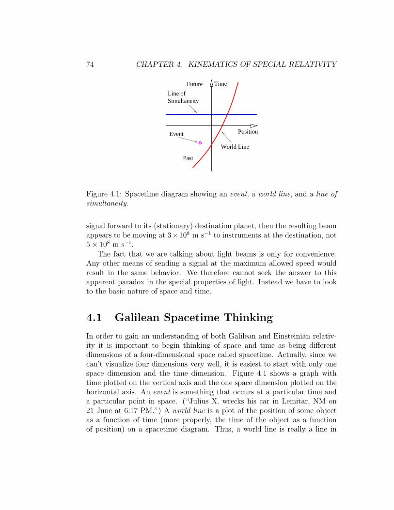
74 CHAPTER 4. KINEMATICS OF SPECIAL RELATIVITY
World Line
Time
Past
PositionEvent
SimultaneityLine of
Future
Figure 4.1: Spacetime diagram showing an event, a world line, and a line of
simultaneity.
signal forward to its (stationary) destination planet, then the resulting beamappears to be moving at 3×10⁸ m s−1 to instruments at the destination, not5 × 108 m s−1.
The fact that we are talking about light beams is only for convenience.Any other means of sending a signal at the maximum allowed speed wouldresult in the same behavior. We therefore cannot seek the answer to thisapparent paradox in the special properties of light. Instead we have to lookto the basic nature of space and time.
4.1 Galilean Spacetime Thinking
In order to gain an understanding of both Galilean and Einsteinian relativ-ity it is important to begin thinking of space and time as being differentdimensions of a four-dimensional space called spacetime. Actually, since wecan’t visualize four dimensions very well, it is easiest to start with only onespace dimension and the time dimension. Figure 4.1 shows a graph withtime plotted on the vertical axis and the one space dimension plotted on thehorizontal axis. An event is something that occurs at a particular time anda particular point in space. (“Julius X. wrecks his car in Lemitar, NM on21 June at 6:17 PM.”) A world line is a plot of the position of some objectas a function of time (more properly, the time of the object as a functionof position) on a spacetime diagram. Thus, a world line is really a line in
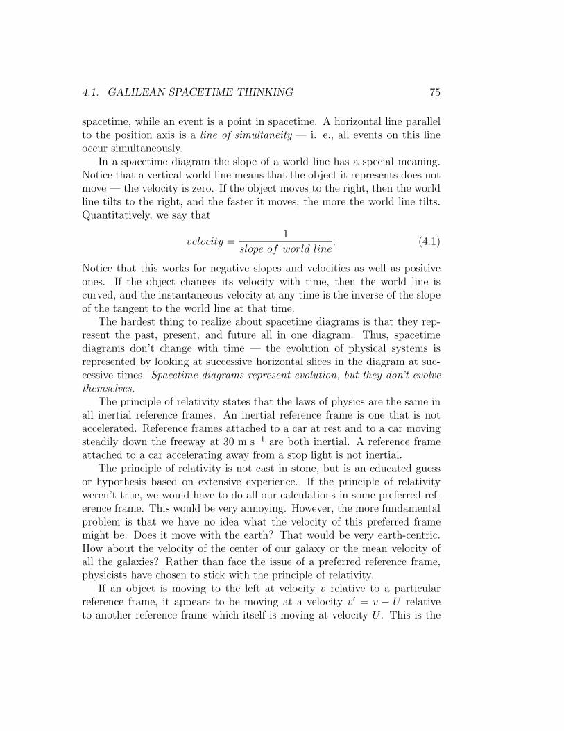
4.1. GALILEAN SPACETIME THINKING 75
spacetime, while an event is a point in spacetime. A horizontal line parallelto the position axis is a line of simultaneity — i. e., all events on this lineoccur simultaneously.
In a spacetime diagram the slope of a world line has a special meaning.Notice that a vertical world line means that the object it represents does notmove — the velocity is zero. If the object moves to the right, then the worldline tilts to the right, and the faster it moves, the more the world line tilts.Quantitatively, we say that
velocity =1
slope of world line. (4.1)
Notice that this works for negative slopes and velocities as well as positiveones. If the object changes its velocity with time, then the world line iscurved, and the instantaneous velocity at any time is the inverse of the slopeof the tangent to the world line at that time.
The hardest thing to realize about spacetime diagrams is that they rep-resent the past, present, and future all in one diagram. Thus, spacetimediagrams don’t change with time — the evolution of physical systems isrepresented by looking at successive horizontal slices in the diagram at suc-cessive times. Spacetime diagrams represent evolution, but they don’t evolve
themselves.
The principle of relativity states that the laws of physics are the same inall inertial reference frames. An inertial reference frame is one that is notaccelerated. Reference frames attached to a car at rest and to a car movingsteadily down the freeway at 30 m s−1 are both inertial. A reference frameattached to a car accelerating away from a stop light is not inertial.
The principle of relativity is not cast in stone, but is an educated guessor hypothesis based on extensive experience. If the principle of relativityweren’t true, we would have to do all our calculations in some preferred ref-erence frame. This would be very annoying. However, the more fundamentalproblem is that we have no idea what the velocity of this preferred framemight be. Does it move with the earth? That would be very earth-centric.How about the velocity of the center of our galaxy or the mean velocity ofall the galaxies? Rather than face the issue of a preferred reference frame,physicists have chosen to stick with the principle of relativity.
If an object is moving to the left at velocity v relative to a particularreference frame, it appears to be moving at a velocity v′ = v − U relativeto another reference frame which itself is moving at velocity U . This is the

76 CHAPTER 4. KINEMATICS OF SPECIAL RELATIVITY
x, x’
t t’
world line of objectmoving at speed v
primed coordsys movingatspeed U
x, x’
t’t
world line of objectmoving at speedv’ = v - U
unprimed coordsys moving atspeed -U
Figure 4.2: The left panel shows the world line in the unprimed referenceframe, while the right panel shows it in the primed frame, which moves tothe right at speed U relative to the unprimed frame. (The “prime” is just alabel that allows us to distinguish the axes corresponding to the two referenceframes.)
Galilean velocity transformation law, and it is based in everyday experience— i. e., if you are traveling 30 m s−1 down the freeway and another carpasses you doing 40 m s−1, then the other car moves past you at 10 m s−1
relative to your car. Figure 4.2 shows how the world line of an object isrepresented differently in the unprimed (x, t) and primed (x′, t′) referenceframes.
4.2 Spacetime Thinking in Special Relativity
In special relativity we find that space and time “mix” in a way that theydon’t in Galilean relativity. This suggests that space and time are differentaspects of the same “thing”, which we call spacetime.
If time and position are simply different dimensions of the same abstractspace, then they should have the same units. The easiest way to arrangethis is to multiply time by the maximum speed, c, resulting in the kind ofspacetime diagram shown in figure 4.3. Notice that world lines of light haveslope ±1 when the time axis is scaled this way. Furthermore, the relationship
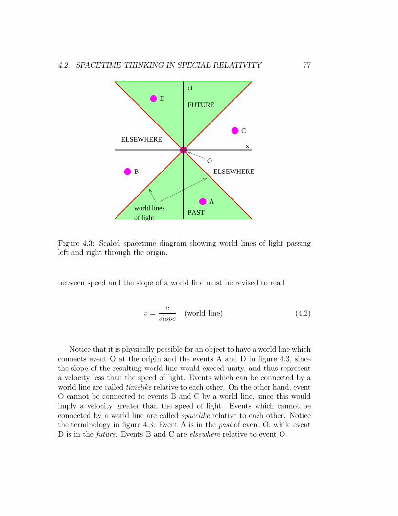
4.2. SPACETIME THINKING IN SPECIAL RELATIVITY 77
ct
x
world linesof light
C
A
B
D
O
FUTURE
PAST
ELSEWHERE
ELSEWHERE
Figure 4.3: Scaled spacetime diagram showing world lines of light passingleft and right through the origin.
between speed and the slope of a world line must be revised to read
v =c
slope(world line). (4.2)
Notice that it is physically possible for an object to have a world line whichconnects event O at the origin and the events A and D in figure 4.3, sincethe slope of the resulting world line would exceed unity, and thus representa velocity less than the speed of light. Events which can be connected by aworld line are called timelike relative to each other. On the other hand, eventO cannot be connected to events B and C by a world line, since this wouldimply a velocity greater than the speed of light. Events which cannot beconnected by a world line are called spacelike relative to each other. Noticethe terminology in figure 4.3: Event A is in the past of event O, while eventD is in the future. Events B and C are elsewhere relative to event O.

78 CHAPTER 4. KINEMATICS OF SPECIAL RELATIVITY
ct
x
A
C
X
IcT
B
Figure 4.4: Triangle for Pythagorean theorem in spacetime.
4.3 Postulates of Special Relativity
As we learned previously, the principle of relativity states that the laws ofphysics are the same in all inertial reference frames. The principle of relativityapplies to Einsteinian relativity just as it applies to Galilean relativity.
Notice that the constancy of the speed of light in all reference framesis consistent with the principle of relativity. However, as noted above, it isinconsistent with our notions as to how velocities add, or alternatively, howwe think the world should look from reference frames moving at differentspeeds. We have called the classical way of understanding the view fromdifferent reference frames Galilean relativity. The new way that reconcilesthe behavior of objects moving at very high speeds is called Einsteinian
relativity. Einstein’s great contribution was to discover the laws that tell ushow the world looks from reference frames moving at high speeds relative toeach other. These laws constitute a geometry of spacetime, and from themall of special relativity can be derived.
All of the observed facts about spacetime can be derived from two pos-tulates:
• Whether two events are simultaneous depends on the reference framefrom which they are viewed.
• Spacetime obeys a modified Pythagorean theorem, which gives the dis-

4.3. POSTULATES OF SPECIAL RELATIVITY 79
x
ct ct’
x’
B
C
X
cT
E D
A
Figure 4.5: Sketch of coordinate axes for a moving reference frame, x′, ct′.The meanings of the events A-E are discussed in the text. The lines tiltedat ±45◦ are the world lines of light passing through the origin.
tance, I, in spacetime as
I2 = X2 − c2T 2, (4.3)
where X, T , and I are defined in figure 4.4.
Let us discuss these postulates in turn.
4.3.1 Simultaneity
The classical way of thinking about simultaneity is so ingrained in our every-day habits that we have a great deal of difficulty adjusting to what specialrelativity has to say about this subject. Indeed, understanding how relativitychanges this concept is the single most difficult part of the theory — onceyou understand this, you are well on your way to mastering relativity!
Before tackling simultaneity, let us first think about collocation. Twoevents (such as A and E in figure 4.5) are collocated if they have the same

80 CHAPTER 4. KINEMATICS OF SPECIAL RELATIVITY
x value. However, collocation is a concept that depends on reference frame.For instance, George is driving from Boston to Washington. Just as he passesNew York he sneezes (event A in figure 4.5). As he drives by Baltimore, hesneezes again (event D). In the reference frame of the earth, these two sneezesare not collocated, since they are separated by many kilometers. However, inthe reference frame of George’s car, they occur in the same place — assumingthat George hasn’t left the driver’s seat!
Notice that any two events separated by a timelike interval are collocatedin some reference frame. The speed of the reference frame is given by equation(4.2), where the slope is simply the slope of the world line connecting thetwo events.
Classically, if two events are simultaneous, we consider them to be simul-taneous in all reference frames. For instance, if two clocks, one in New Yorkand one in Los Angeles, strike the hour at the same time in the earth refer-ence frame, then classically these events also appear to be simultaneous toinstruments in the space shuttle as it flies over the United States. However,if the space shuttle is moving from west to east, i. e., from Los Angeles to-ward New York, careful measurements will show that the clock in New Yorkstrikes the hour before the clock in Los Angeles!
Just as collocation depends on one’s reference frame, this result showsthat simultaneity also depends on reference frame. Figure 4.5 shows howthis works. In figure 4.5 events A and B are simultaneous in the rest orunprimed reference frame. However, in the primed reference frame, events Aand C are simultaneous, and event B occurs at an earlier time. If A and Bcorrespond to the clocks striking in Los Angeles and New York respectively,then it is clear that B must occur at an earlier time in the primed frame ifindeed A and C are simultaneous in that frame.
The tilted line passing through events A and C in figure 4.5 is called theline of simultaneity for the primed reference frame. Its slope is related to thespeed, U , of the reference frame by
slope = U/c (line of simultaneity). (4.4)
Notice that this is the inverse of the slope of the world line attached to theprimed reference frame. There is thus a symmetry between the world lineand the line of simultaneity of a moving reference frame — as the referenceframe moves faster to the right, these two lines close like the blades of a pairof scissors on the 45◦ line.

4.3. POSTULATES OF SPECIAL RELATIVITY 81
x
ctct
x
A B
A
B
O1 O2 O1 O2S S
Stationary source and observers Moving source and observers
X X
Figure 4.6: World lines of two observers (O1, O2) and a pulsed light source(S) equidistant between them. In the left frame the observers and the sourceare all stationary. In the right frame they are all moving to the right at halfthe speed of light. The dashed lines show pulses of light emitted simultane-ously to the left and the right.
In Galilean relativity it is fairly obvious what we mean by two events beingsimultaneous — it all boils down to coordinating portable clocks which aresitting next to each other, and then moving them to the desired locations.Two events separated in space are simultaneous if they occur at the sametime on clocks located near each event, assuming that the clocks have beencoordinated in the above manner.
In Einsteinian relativity this doesn’t work, because the very act of movingthe clocks changes the rate at which the clocks run. Thus, it is more difficultto determine whether two distant events are simultaneous.
An alternate way of experimentally determining simultaneity is shown infigure 4.6. Since we know from observation that light travels at the samespeed in all reference frames, the pulses of light emitted by the light sourcesin figure 4.6 will reach the two equidistant observers simultaneously in bothcases. The line passing through these two events, A and B, defines a line ofsimultaneity for both stationary and moving observers. For the stationaryobservers this line is horizontal, as in Galilean relativity. For the movingobservers the light has to travel farther in the rest frame to reach the observerreceding from the light source, and it therefore takes longer in this frame.Thus, event B in the right panel of figure 4.6 occurs later than event A in

82 CHAPTER 4. KINEMATICS OF SPECIAL RELATIVITY
the stationary reference frame and the line of simultaneity is tilted. We seethat the postulate that light moves at the same speed in all reference framesleads inevitably to the dependence of simultaneity on reference frame.
4.3.2 Spacetime Pythagorean Theorem
The Pythagorean theorem of spacetime differs from the usual Pythagoreantheorem in two ways. First, the vertical side of the triangle is multiplied by c.This is a trivial scale factor that gives time the same units as space. Second,the right side of equation (4.3) has a minus sign rather than a plus sign. Thishighlights a fundamental difference between spacetime and the ordinary xyzspace in which we live. Spacetime is said to have a non-Euclidean geometry— in other words, the normal rules of geometry that we learn in high schooldon’t always work for spacetime!
The main consequence of the minus sign in equation (4.3) is that I2 canbe negative and therefore I can be imaginary. Furthermore, in the specialcase where X = ±cT , we actually have I = 0 even though X, T 6= 0 — i.e., the “distance” between two well-separated events can be zero. Clearly,spacetime has some weird properties!
The quantity I is usually called an interval in spacetime. Generally speak-ing, if I2 is positive, the interval is called spacelike, while for a negative I2,the interval is called timelike.
A concept related to the spacetime interval is the proper time τ . Theproper time between the two events A and C in figure 4.4 is defined by theequation
τ 2 = T 2 −X2/c2. (4.5)
Notice that I and τ are related by
τ 2 = −I2/c2, (4.6)
so the spacetime interval and the proper time are not independent concepts.However, I has the dimensions of length and is real when the events definingthe interval are spacelike relative to each other, whereas τ has the dimen-sions of time and is real when the events are timelike relative to each other.Both equation (4.3) and equation (4.5) express the spacetime Pythagoreantheorem.
If two events defining the end points of an interval have the same t value,then the interval is the ordinary space distance between the two events. On

4.4. TIME DILATION 83
ct
x’
x
ct’ ct ct’
x’
x
A A
View fromstationaryframe
View fromco-movingframe
BC B
CX
cT’cT’ cT
X
cT
Figure 4.7: Two views of the relationship between three events, A, B, and C.The left panel shows the view from the unprimed reference frame, in which Aand C are collocated, while the right panel shows the view from the primedframe, in which A and B are collocated.
the other hand, if they have the same x value, then the proper time is justthe time interval between the events. If the interval between two events isspacelike, but the events are not simultaneous in the initial reference frame,they can always be made simultaneous by choosing a reference frame inwhich the events lie on the same line of simultaneity. Thus, the meaning ofthe interval in that case is just the distance between the events in the newreference frame. Similarly, for events separated by a timelike interval, theproper time is just the time between two events in a reference frame in whichthe two events are collocated.
4.4 Time Dilation
Stationary and moving clocks run at different rates in relativity. This isillustrated in figure 4.7. The triangle ABC in the left panel of figure 4.7can be used to illustrate this point. Suppose that the line passing throughthe events A and C in this figure is the world line of a stationary observer.At zero time another observer moving with velocity V passes the stationaryobserver. The moving observer’s world line passes through events A and B.

84 CHAPTER 4. KINEMATICS OF SPECIAL RELATIVITY
We assume that events B and C are simultaneous in the rest frame, soABC is a right triangle. Application of the spacetime Pythagorean theoremthus yields
c2T ′2 = c2T 2 −X2. (4.7)
Since the second observer is moving at velocity V , the slope of his world lineis
c
V=cT
X, (4.8)
where the right side of the above equation is the slope calculated as the riseof the world line cT over the run X between events A and B. Eliminating Xbetween the above two equations results in a relationship between T and T ′:
T ′ = T (1 − V 2/c2)1/2 ≡ T/γ, (4.9)
where
γ =1
(1 − V 2/c2)1/2. (4.10)
The quantity γ occurs so often in relativistic calculations that we give it thisspecial name. Note by its definition that γ ≥ 1.
Equation (4.9) tells us that the time elapsed for the moving observer isless than that for the stationary observer, which means that the clock of themoving observer runs more slowly. This is called the time dilation effect.
Let us view this situation from the reference frame of the moving observer.In this frame the moving observer becomes stationary and the stationaryobserver moves in the opposite direction, as illustrated in the right panel offigure 4.7. By symmetric arguments, one infers that the clock of the initiallystationary observer who is now moving to the left runs more slowly in thisreference frame than the clock of the initially moving observer. One mightconclude that this contradicts the previous results. However, examinationof the right panel of figure 4.7 shows that this is not so. The interval cT isstill greater than the interval cT ′, because such intervals are relativisticallyinvariant quantities. However, events B and C are no longer simultaneous,so one cannot use these results to infer anything about the rate at whichthe two clocks run in this frame. Thus, the relative nature of the concept ofsimultaneity saves us from an incipient paradox, and we see that the relativerates at which clocks run depends on the reference frame in which these ratesare observed.

4.5. LORENTZ CONTRACTION 85
ct’
x’
x
A
ct ct ct’
A
cT’X
cT’
B
Co-movingframe
Stationaryframe
C
x’
xB
C
X’
X’
X
Figure 4.8: Definition sketch for understanding the Lorentz contraction. Theparallel lines represent the world lines of the front and the rear of a movingobject. The left panel shows a reference frame moving with the object, whilethe right panel shows a stationary reference frame.
4.5 Lorentz Contraction
A similar argument can be made to show how the postulates of relativityresult in the Lorentz contraction. Figure 4.8 compares the length X ′ of amoving object measured in its own reference frame (left panel) with its lengthX as measured in a stationary reference frame (right panel). The lengthof a moving object is measured by simultaneously measuring the positionsof the front and the rear of the object and subtracting these two numbers.Events A and C correspond to these position measurements for the stationaryreference frame since they are respectively on the rear and front world linesof the object. Thus, the interval AC, which is equal to X, is the length ofthe object as measured in the stationary frame.
In the left panel, X is the hypotenuse of a right triangle. Therefore, bythe Pythagorean theorem of spacetime, we have
X = I = (X ′2 − c2T ′2)1/2. (4.11)
Now, the line passing through A and C in the left panel is the line of si-multaneity of the stationary reference frame. The slope of this line is −V/c,where V is the speed of the object relative to the stationary reference frame.

86 CHAPTER 4. KINEMATICS OF SPECIAL RELATIVITY
x
ct
world lineof stationarytwin
world line oftravelingtwin
O
A
B
C
Figure 4.9: Definition sketch for the twin paradox. The vertical line is theworld line of the twin that stays at home, while the traveling twin has thecurved world line to the right. The slanted lines between the world linesare lines of simultaneity at various times for the traveling twin. The heavylines of simultaneity bound the period during which the traveling twin isdecelerating to a stop and accelerating toward home.
Geometrically in figure 4.8, the slope of this line is −cT ′/X ′, so we find byequating these two expressions for the slope that
T ′ = V X ′/c2. (4.12)
Finally, eliminating T ′ between (4.11) and (4.12) results in
X = X ′(1 − V 2/c2)1/2 = X ′/γ. (4.13)
This says that the length of a moving object as measured in a stationaryreference frame (X) is less than the actual length of the object as measuredin its own reference frame (X ′). This apparent reduction in length is calledthe Lorentz contraction.
4.6 Twin Paradox
An interesting application of time dilation is the so-called twin paradox, whichturns out not to be a paradox at all. Two twins are initially the same age.

4.7. PROBLEMS 87
One twin travels to a distant star on an interstellar spaceship which movesat speed V , which is close to the speed of light. Upon reaching the star, thetraveling twin immediately turns around and heads home. When reachinghome, the traveling twin has aged less than the twin that stayed home. Thisis easily explained by the time dilation effect, which shows that the propertime elapsed along the world line of the traveling twin is (1−V 2/c2)1/2 timesthe proper time elapsed along the world line of the other twin.
The “paradox” part of the twin paradox arises from making the symmetricargument in which one assumes the reference frame of the traveling twin to bestationary. The frame of the earth-bound twin must then travel in the senseopposite that of the erstwhile traveling twin, which means that the earth-bound twin must age less rather than more. This substitution is justified onthe basis of the principle of relativity, which states that the laws of physicsmust be the same in all inertial reference frames.
However, the above argument is fallacious, because the reference frame ofthe traveling twin is not inertial throughout the entire trip, since at variouspoints the spaceship has to accelerate and decelerate. Thus, the principle ofrelativity cannot be used to assert the equivalence of the traveler’s referenceframe to the stationary frame.
Of particular importance is the period of deceleration and accelerationnear the distant star. During this interval, the line of simulaneity of thetraveling twin rotates, as illustrated in figure 4.9, such that the twin stayingat home rapidly ages in the reference frame of the traveler. Thus, eventhough the acceleration of the traveling twin may occupy only a negligiblesegment of the twin’s world line, the overall effect is not negligible. In fact,the shorter and more intense the period of acceleration, the more rapidly theearth-bound twin ages in the traveling frame during this interval!
4.7 Problems
1. Sketch your personal world line on a spacetime diagram for the last24 hours, labeling by time and location special events such as meals,physics classes, etc. Relate the slope of the world line at various timesto how fast you were walking, riding in a car, etc.
2. Spacetime conversions:
(a) What is the distance from New York to Los Angeles in seconds?

88 CHAPTER 4. KINEMATICS OF SPECIAL RELATIVITY
From here to the moon? From here to the sun?
(b) What is one nanosecond in meters? One second? One day? Oneyear?
3. Three events have the following spacetime coordinates: A is at (x, ct) =(2 m, 1 m); B is at (x, ct) = (−2 m, 0 m); C is at (x, ct) = (0 m, 3 m).
(a) A world line for an object passes through events B and C. Howfast and in which direction is the object moving?
(b) A line of simultaneity for a coordinate system passes throughevents A and B. How fast and in which direction is the coordi-nate system moving?
(c) What is the invariant interval between events A and B? B and C?A and C?
(d) Can a signal from event B reach event A? Can it reach event C?Explain.
Hint: Draw a spacetime diagram with all the events plotted beforetrying to answer the above questions.
4. In the following problem be sure to indicate the slope of all pertinentlines drawn.
(a) In a spacetime diagram, sketch a line of simultaneity for a referenceframe moving to the left at V = c/2, where c is the speed of light.
(b) Sketch the world line of an object which is initially stationary, butwhich accelerates to a velocity of v = c/3.
(c) If the slopes of the world lines of the observers in the right panel offigure 4.6 are both 1/β, find the slope of their line of simultaneity,AB.
5. Suppose that an interstellar spaceship goes a distanceX = 100 light yearsrelative to the rest frame in T ′ = 10 years of its own time.
(a) Draw a spacetime diagram in the rest frame showing X, T ′, andthe time T needed for this journey relative to the rest frame.
(b) Compute T , using your spacetime diagram as an aid.

4.7. PROBLEMS 89
(c) Compute the speed of the spaceship.
6. If an airline pilot flies 80 hr per month (in the rest frame) at 300 m s−1
for 30 years, how much younger will she be than her twin brother (whohandles baggage) when she retires? Hint: Use (1 − ǫ)x ≈ 1 − xǫ forsmall ǫ.
7. A mu particle normally lives about 2×10⁻⁶ sec before it decays. How-ever, muons created by cosmic rays 20 km up in the atmosphere reachthe Earth’s surface. How fast must they be going?
8. The Stanford Linear Accelerator accelerates electrons to a speed suchthat the 3 km long accelerator appears to be 8 cm long to the electron,due to the Lorentz contraction. How much less than the speed oflight is the electron traveling? Hint: It is best to first develop anapproximation for the relationship between γ = (1−v2/c2)−1/2 and thedifference between c and v for a particle moving close to the speed oflight.
9. How fast do you have to go to reach the center of our galaxy in yourexpected lifetime? At this speed, what does this distance appear tobe? (We are about 30000 ly from the galactic center.)
10. Two identical spaceships pass each other going in the opposite directionat the same speed.
(a) Sketch a spacetime diagram showing the world lines of the frontand rear of each spaceship.
(b) Indicate an interval on the diagram corresponding to the rightward-moving spaceship’s length in its own reference frame.
(c) Indicate an interval corresponding to the leftward-moving space-ship’s length in the reference frame of the rightward-moving space-ship.
(d) Indicate an interval equal to the length of either spaceship in therest frame.
11. George and Sally are identical twins initially separated by a distance dand at rest. In the rest frame they are initially the same age. At timet = 0 both George and Sally get in their spaceships and head to the
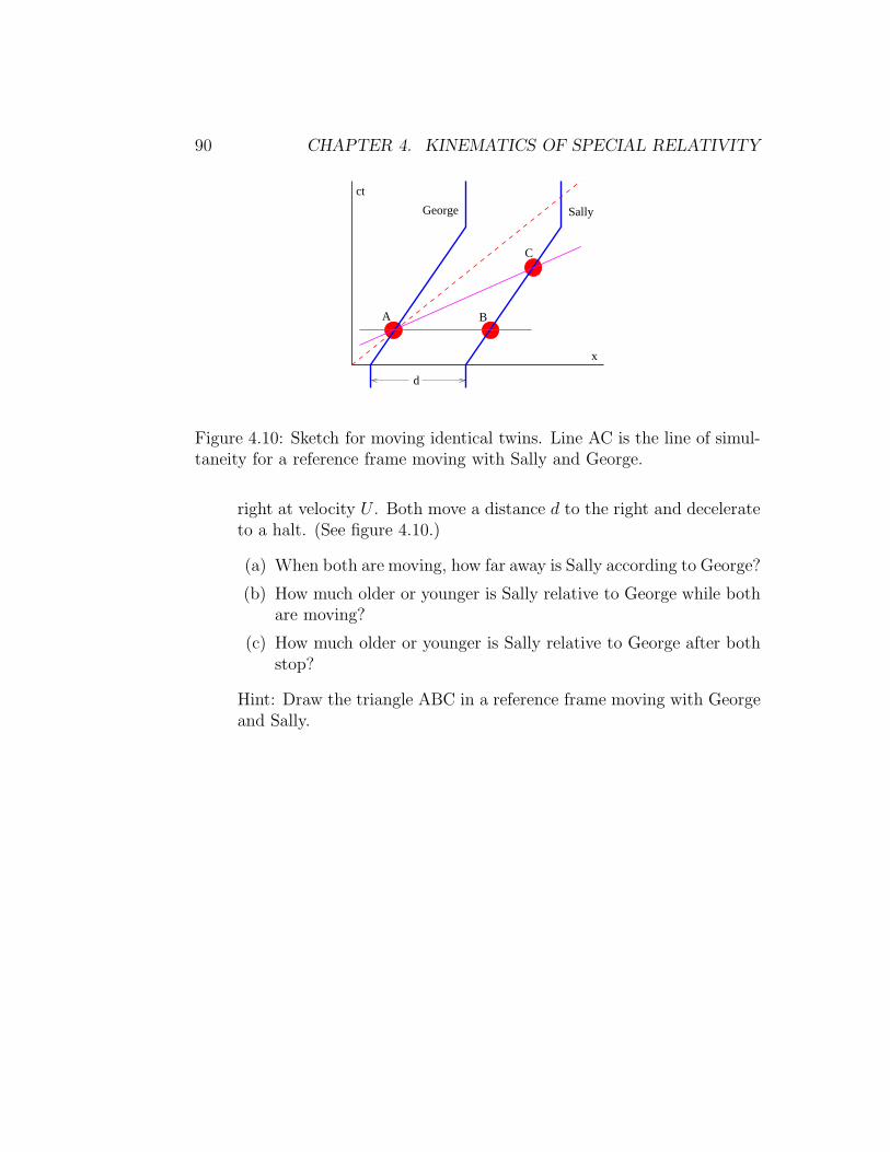
90 CHAPTER 4. KINEMATICS OF SPECIAL RELATIVITY
x
ct
A B
C
d
SallyGeorge
Figure 4.10: Sketch for moving identical twins. Line AC is the line of simul-taneity for a reference frame moving with Sally and George.
right at velocity U . Both move a distance d to the right and decelerateto a halt. (See figure 4.10.)
(a) When both are moving, how far away is Sally according to George?
(b) How much older or younger is Sally relative to George while bothare moving?
(c) How much older or younger is Sally relative to George after bothstop?
Hint: Draw the triangle ABC in a reference frame moving with Georgeand Sally.
Chapter 5
Applications of Special
Relativity
In this chapter we continue the study of special relativity. Three importantapplications of the ideas developed in the previous chapter are made here.First, we show how to describe waves in the context of spacetime. We thensee how waves which have no preferred reference frame (such as that of amedium supporting them) are constrained by special relativity to have adispersion relation of a particular form. This dispersion relation turns out tobe that of the relativistic matter waves of quantum mechanics. Second, weinvestigate the Doppler shift phenomenon, in which the frequency of a wavetakes on different values in different coordinate systems. Third, we show howto add velocities in a relativistically consistent manner.
A new mathematical idea is presented in the context of relativistic waves,namely the spacetime vector or four-vector. Writing the laws of physicstotally in terms of relativistic scalars and four-vectors insures that they willbe valid in all inertial reference frames.
5.1 Waves in Spacetime
We now look at the characteristics of waves in spacetime. Recall that a wavein one space dimension can be represented by
A(x, t) = A0 sin(kx− ωt), (5.1)
where A0 is the (constant) amplitude of the wave, k is the wavenumber, andω is the angular frequency, and that the quantity φ = kx − ωt is called
91

92 CHAPTER 5. APPLICATIONS OF SPECIAL RELATIVITY
Wave4-vector
/cω
ct
x
Wave fronts
k
Figure 5.1: Sketch of wave fronts for a wave in spacetime. The large arrowis the associated wave four-vector, which has slope ω/ck. The slope of thewave fronts is the inverse, ck/ω. The phase speed of the wave is greater thanc in this example. (Can you tell why?)
the phase of the wave. For a wave in three space dimensions, the wave isrepresented in a similar way,
A(x, t) = A0 sin(k · x − ωt), (5.2)
where x is now the position vector and k is the wave vector. The magnitude ofthe wave vector, |k| = k is just the wavenumber of the wave and the directionof this vector indicates the direction the wave is moving. The phase of thewave in this case is φ = k · x − ωt.
In the one-dimensional case φ = kx−ωt. A wave front has constant phaseφ, so solving this equation for t and multiplying by c, the speed of light in avacuum, gives us an equation for the world line of a wave front:
ct =ckx
ω−cφ
ω=cx
up
−cφ
ω(wave front). (5.3)
The slope of the world line in a spacetime diagram is the coefficient of x, orc/up, where up = ω/k is the phase speed.
5.2 Math Tutorial – Four-Vectors
Also shown in figure 5.1 is a spacetime vector or four-vector which representsthe frequency and wavenumber of the wave, which we refer to as the wave

5.2. MATH TUTORIAL – FOUR-VECTORS 93
four-vector. It is called a four-vector because it has 3 spacelike componentsand one timelike component when there are 3 space dimensions. In the caseshown, there is only a single space dimension. The spacelike component ofthe wave four-vector is just k (or k when there are 3 space dimensions),while the timelike component is ω/c. The c is in the denominator to give thetimelike component the same dimensions as the spacelike component. Fromfigure 5.1 it is clear that the slope of the line representing the four-vector isω/ck, which is just the inverse of the slope of the wave fronts.
Let us define some terminology. We indicate a four-vector by underliningand write the components in the following way: k = (k, ω/c), where k isthe wave four-vector, k is its spacelike component, and ω/c is its timelikecomponent. For three space dimensions, where we have a wave vector ratherthan just a wavenumber, we write k = (k, ω/c).
Another example of a four-vector is simply the position vector in space-time, x = (x, ct), or x = (x, ct) in three space dimensions. The c multiplies
the timelike component in this case, because that is what is needed to giveit the same dimensions as the spacelike component.
In three dimensions we define a vector as a quantity with magnitudeand direction. Extending this to spacetime, a four-vector is a quantity withmagnitude and direction in spacetime. Implicit in this definition is the notionthat the vector’s magnitude is a quantity independent of coordinate systemor reference frame. We have seen that the invariant interval in spacetime isI = (x2 − c2t2)1/2, so it makes sense to identify this as the magnitude of theposition vector. This leads to a way of defining a dot product of four-vectors.Given two four-vectors A = (A, At) and B = (B, Bt), the dot product is
A ·B = A ·B − AtBt (dot product in spacetime). (5.4)
This is consistent with the definition of invariant interval if we set A = B = x,since then x · x = x2 − c2t2 = I2.
In the odd geometry of spacetime it is not obvious what “perpendicular”means. We therefore define two four-vectors A and B to be perpendicular iftheir dot product is zero: A ·B = 0.
The dot product of two four-vectors is a scalar result, i. e., its valueis independent of coordinate system. This can be used to advantage onoccasion. For instance, consider the dot product of a four-vector A whichresolves into (Ax, At) in the unprimed frame. Let us further suppose that thespacelike component is zero in some primed frame, so that the components

94 CHAPTER 5. APPLICATIONS OF SPECIAL RELATIVITY
in this frame are (0, A′
t). The fact that the dot product is independent ofcoordinate system means that
A · A = A2
x − A2
t = −A′2
t . (5.5)
This constitutes an extension of the spacetime Pythagorean theorem to four-vectors other than the position four-vector. Thus, for instance, the wavenum-ber for some wave may be zero in the primed frame, which means that thewavenumber and frequency in the unprimed frame are related to the fre-quency in the primed frame by
k2 − ω2/c2 = −ω′2/c2. (5.6)
5.3 Principle of Relativity Applied
Returning to the phase of a wave, we immediately see that
φ = k · x − ωt = k · x − (ω/c)(ct) = k · x. (5.7)
Thus, a compact way to rewrite equation (5.2) is
A(x) = sin(k · x). (5.8)
Since x is known to be a four-vector and since the phase of a wave isknown to be a scalar independent of reference frame, it follows that k is alsoa four-vector rather than just a set of numbers. Thus, the square of thelength of the wave four-vector must also be a scalar independent of referenceframe:
k · k = k · k − ω2/c2 = const. (5.9)
Let us review precisely what this means. As figure 5.2 shows, we can re-solve a position four-vector into components in two different reference frames,x = (X, cT ) = (X ′, cT ′). However, even though X 6= X ′ and T 6= T ′, thevector lengths computed from these two sets of components are necessarilythe same: x · x = X2 − c2T 2 = X ′2 − c2T ′2.
Applying this to the wave four-vector, we infer that
k2 − ω2/c2 = k′2 − ω′2/c2 = const., (5.10)
where the unprimed and primed values of k and ω refer to the componentsof the wave four-vector in two different reference frames.

5.3. PRINCIPLE OF RELATIVITY APPLIED 95
x
ct’ct
X
x’
cT
X’
cT’
Figure 5.2: Resolution of a four-vector into components in two differentreference frames.
Up to now, this argument applies to any wave. However, waves canbe divided into two categories, those for which a “special” reference frameexists, and those for which there is no such special frame. As an example ofthe former, sound waves look simplest in the reference frame in which thegas carrying the sound is stationary. The same is true of light propagatingthrough a material medium with an index of refraction not equal to unity.In both cases the speed of the wave is the same in all directions only in theframe in which the material medium is stationary.
The following argument can be made. Suppose we have a machine thatproduces a wave with wavenumber k and frequency ω in its own rest frame.If we observe the wave from a moving reference frame, the wavenumber andfrequency will be different, say, k′ and ω′. However, these quantities will berelated by equation (5.10).
Up to this point the argument applies to any wave whether a special refer-ence frame exists or not; the observed changes in wavenumber and frequencyhave nothing to do with the wave itself, but are just consequences of how wehave chosen to observe it. However, if there is no special reference frame forthe type of wave under consideration, then the same result can be obtainedby keeping the observer stationary and moving the wave-producing machinein the opposite direction. By moving it at various speeds, any desired valueof k′ can be obtained in the initial reference frame (as opposed to some otherframe), and the resulting value of ω′ can be computed using equation (5.10).
This is actually an amazing result. We have shown on the basis of the

96 CHAPTER 5. APPLICATIONS OF SPECIAL RELATIVITY
principle of relativity that any wave type for which no special reference frameexists can be made to take on a full range of frequencies and wavenumbersin any given reference frame, and furthermore that these frequencies andwavenumbers obey
ω2 = k2c2 + µ2. (5.11)
Equation (5.11) comes from solving equation (5.10) for ω2 and the constantµ2 equals the constant in equation (5.10) times −c2. Equation (5.11) relatesfrequency to wavenumber and therefore is the dispersion relation for suchwaves. We call waves which have no special reference frame and thereforenecessarily obey equation (5.11) relativistic waves. The only difference in thedispersion relations between different types of relativistic waves is the valueof the constant µ. The meaning of this constant will become clear later.
5.4 Characteristics of Relativistic Waves
Light in a vacuum is an example of a wave for which no special referenceframe exists. For light, µ = 0, and we have (taking the positive root) ω = ck.This simply states what we know already, namely that the phase speed oflight in a vacuum is c.
If µ 6= 0, waves of this type are dispersive. The phase speed is
up =ω
k= (c2 + µ2/k2)1/2. (5.12)
This phase speed always exceeds c, which at first seems like an unphysicalconclusion. However, the group velocity of the wave is
ug =dω
dk=
c2k
(k2c2 + µ2)1/2=kc2
ω=c2
up, (5.13)
which is always less than c. Since wave packets and hence signals propagateat the group velocity, waves of this type are physically reasonable even thoughthe phase speed exceeds the speed of light.
Another interesting property of such waves is that the wave four-vector isparallel to the world line of a wave packet in spacetime. This is easily shownby the following argument. As figure 5.1 shows, the spacelike componentof a wave four-vector is k, while the timelike component is ω/c. The slopeof the four-vector on a spacetime diagram is therefore ω/kc. However, the

5.5. THE DOPPLER EFFECT 97
wave fronts
world line of movingobserver
cT’ cτ
ct
x
X
cT
X
world line ofstationarysource
Figure 5.3: Definition sketch for computing the Doppler effect for light.
slope of the world line of a wave packet moving with group velocity ug isc/ug = ω/(kc).
Note that when k = 0 we have ω = µ. In this case the group velocity ofthe wave is zero. For this reason we call µ the rest frequency of the wave.
5.5 The Doppler Effect
You have probably heard how the pitch of a train horn changes as it passesyou. When the train is approaching, the pitch or frequency is higher thanwhen it is moving away from you. This is called the Doppler effect. Asimilar, but distinct effect occurs if you are moving past a source of sound.If a stationary whistle is blowing, the pitch perceived from a moving car ishigher while moving toward the source than when moving away. The firstcase thus has a moving source, while the second case has a moving observer.
In this section we compute the Doppler effect as it applies to light movingthrough a vacuum. Figure 5.3 shows the geometry for computing the timebetween wave fronts of light for a stationary and a moving reference frame.The time in the stationary frame is just T . Since the world lines of the wavefronts have a slope of unity, the sides of the shaded triangle have the samevalue, X. If the observer is moving at speed U , the slope of the observer’s

98 CHAPTER 5. APPLICATIONS OF SPECIAL RELATIVITY
world line is c/U , which means that c/U = (cT +X)/X. Solving this for Xyields X = UT/(1−U/c), which can then be used to compute T ′ = T+X/c =T/(1−U/c). This formula as it stands leads to the classical Doppler shift fora moving observer. However, with relativistic velocities, one additional factorneeds to be taken in into account: The observer experiences time dilationsince he or she is moving. The actual time measured by the observer betweenwave fronts is actually
τ = (T ′2 −X2/c2)1/2 = T(1 − U2/c2)1/2
1 − U/c= T
(
1 + U/c
1 − U/c
)1/2
, (5.14)
where the last step uses 1−U2/c2 = (1−U/c)(1 +U/c). From this we inferthe relativistic Doppler shift formula for light in a vacuum:
ω′ = ω
(
1 − U/c
1 + U/c
)1/2
, (5.15)
where the frequency measured by the moving observer is ω′ = 2π/τ and thefrequency observed in the stationary frame is ω = 2π/T .
We could go on to determine the Doppler shift resulting from a movingsource. However, by the principle of relativity, the laws of physics shouldbe the same in the reference frame in which the observer is stationary andthe source is moving. Furthermore, the speed of light is still c in that frame.Therefore, the problem of a stationary observer and a moving source is con-ceptually the same as the problem of a moving observer and a stationarysource when the wave is moving at speed c. This is unlike the case for, say,sound waves, where the stationary observer and the stationary source yielddifferent formulas for the Doppler shift.
5.6 Addition of Velocities
Figure 5.4 shows the world line of a moving object from the point of view oftwo different reference frames, with the primed frame (left panel) moving tothe right at speed U relative to the unprimed frame (right panel). The goalis to calculate the velocity of the object relative to the unprimed frame, v,assuming its velocity in the primed frame, v′ is known. The classical resultis simply
v = U + v′ (classical result). (5.16)

5.6. ADDITION OF VELOCITIES 99
ct’
∆c T
X∆
x’ xO O
A B
B
x’cT’
X’
cT’
A
X’
Boost by U = X/T
X
cT
E
D
World line(velocity v’)
World line(velocity v)
ct’ ct
Figure 5.4: Definition sketch for relativistic velocity addition. The two panelsshow the world line of a moving object relative to two different referenceframes moving at velocity U with respect to each other. The velocity of theworld line in the left panel is v′ while its velocity in the right panel is v.
However, this is inconsistent with the speed of light being constant in allreference frames, since if we substitute c for v′, this formula predicts that thespeed of light in the unprimed frame is U + c.
We can use the geometry of figure 5.4 to come up with the correct rela-tivistic formula. From the right panel of this figure we infer that
v
c=
X + ∆X
cT + c∆T=X/(cT ) + ∆X/(cT )
1 + ∆T/T. (5.17)
This follows from the fact that the slope of the world line of the object inthis frame is c/v. The slope is calculated as the ratio of the rise, c(T + ∆T ),to the run, X + ∆X.
From the left panel of figure 5.4 we similarly see that
v′
c=X ′
cT ′. (5.18)
However, we can apply our calculations of Lorentz contraction and timedilation from the previous chapter to triangles ABD and OAE in the rightpanel. The slope of AB is U/c because AB is horizontal in the left panel, soX ′ = ∆X(1−U2/c2)1/2. Similarly, the slope of OA is c/U since OA is vertical

100 CHAPTER 5. APPLICATIONS OF SPECIAL RELATIVITY
in the left panel, and T ′ = T (1−U2/c2)1/2. Substituting these formulas intothe equation for v′/c yields
v′
c=
∆X
cT. (5.19)
Again using what we know about the triangles ABD and OAE, we see that
U
c=c∆T
∆X=X
cT. (5.20)
Finally, we calculate ∆T/T by noticing that
∆T
T=
∆T
T
c∆X
c∆X=(
c∆T
∆X
)(
∆X
cT
)
=U
c
v′
c. (5.21)
Substituting equations (5.19), (5.20), and (5.21) into equation (5.17) andsimplifying yields the relativistic velocity addition formula:
v =U + v′
1 + Uv′/c2(special relativity). (5.22)
Notice how this equation behaves in various limits. If |Uv′| ≪ c2, thedenominator of equation (5.22) is nearly unity, and the special relativisticformula reduces to the classical case. On the other hand, if v′ = c, thenequation (5.22) reduces to v = c. In other words, if the object in questionis moving at the speed of light in one reference frame, it is moving at thespeed of light in all reference frames, i. e., for all possible values of U . Thus,we have found a velocity addition formula that 1) reduces to the classicalformula for low velocities and 2) gives the observed results for very highvelocities as well.
5.7 Problems
1. Sketch the wave fronts and the k four-vector in a spacetime diagram forthe case where ω/k = 2c. Label your axes and space the wave frontscorrectly for the case k = 4π m−1.
2. If the four-vector k = (0, 1 nm−1) in the rest frame, find the space andtime components of k in a frame moving to the left at speed c/2.
3. Let’s examine the four-vector u = (ug, c)/(1 − β2)1/2 where β = ug/c,ug being the velocity of some object.

5.7. PROBLEMS 101
wave fronts
c τ
x
ct
cT’cT
X
X
world line of stationaryobserver
world line ofmoving source
Figure 5.5: Doppler effect for a moving light source.
(a) Show that u is parallel to the world line of the object.
(b) Show that u · u = −c2.
(c) If ug is the group velocity of a relativistic wave packet, show thatk = (µ/c2)u, where k is the central wave four-vector of the wavepacket.
The four-vector u is called the four-velocity.
4. Find the Doppler shift for a moving source of light from figure 5.5,roughly following the procedure used in the text to find the shift for amoving observer. (Assume that the source moves to the left at speedU .) Is the result the same as for the moving observer, as demanded bythe principle of relativity?
5. Suppose you shine a laser with frequency ω and wavenumber k on amirror moving toward you at speed v, as seen in figure 5.6. Whatare the frequency ω′ and wavenumber k′ of the reflected beam? Hint:Find the frequency of the incident beam in the reference frame of themirror. The frequency of the reflected beam will be the same as that ofthe incident beam in this frame. Then transform back to the referenceframe of the laser.

102 CHAPTER 5. APPLICATIONS OF SPECIAL RELATIVITY
’ωk’,
ωk,
v
v
incident beam
reflected beam
laser
mirror
Figure 5.6: Laser beam reflecting off of a moving mirror.
6. Suppose the moving twin in the twin paradox has a powerful telescopeso that she can watch her twin brother back on earth during the entiretrip. Describe how the earthbound twin appears to age to the travellingtwin compared to her own rate of aging. Use a spacetime diagram toillustrate your argument and consider separately the outbound andreturn legs. Remember that light travels at the speed of light! Hint:Does the concept of Doppler shift help here?
7. Find the velocity of an object with respect to the rest frame if it ismoving at a velocity of 0.1c with respect to another frame which itselfis moving at 0.1c relative to the rest frame using
(a) the Galilean formula and
(b) the formula of special relativity.
Determine the fractional error made in using the Galilean formula.
8. Each stage of a high performance 3 stage rocket can accelerate to aspeed of 0.9c from rest. If the rocket starts from rest, how fast doesthe final stage eventually go?
9. An interstellar spaceship is going from Earth to Sirius with speed U =0.8c relative to the rest frame. It passes a spaceship which is going fromSirius to Earth at a speed of 0.95c in the reference frame of the firstspaceship. What is the velocity (direction and speed) of the secondspaceship in the rest frame?

Chapter 6
Acceleration and General
Relativity
General relativity is Einstein’s extension of special relativity to include grav-ity. An important aspect of general relativity is that spacetime is no longernecessarily flat, but in fact may be curved under the influence of mass. Un-derstanding curved spacetime is an advanced topic which is not easily acces-sible at the level of this course. However, it turns out that some insight intogeneral relativistic phenomena may be obtained by investigating the effectsof acceleration in the flat (but non-Euclidean) space of special relativity.
The central assumption of general relativity is the equivalence principle,which states that gravity is a force which arises from being in an acceleratedreference frame. To understand this we must first investigate the concept ofacceleration. We then see how this leads to phenomena such as the gravi-tational red shift, event horizons, and black holes. We also introduce in apreliminary way the notions of force and mass.
6.1 Acceleration
Imagine that you are in a powerful luxury car stopped at a stoplight. Asyou sit there, gravity pushes you into the comfortable leather seat. The lightturns green and you “floor it”. The car accelerates and and an additionalforce pushes you into the seat back. You round a curve, and yet anotherforce pushes you toward the outside of the curve. (But the well designed seatand seat belt keep you from feeling discomfort!)
103

104 CHAPTER 6. ACCELERATION AND GENERAL RELATIVITY
a
∆tv
∆θ
Linear Motion
A
B
O
CD
E
t
x
v
a ∆t
v
v
∆θ
v
r r
Circular Motion
Figure 6.1: Definition sketches for linear and circular motion.
Let us examine the idea of acceleration more closely. Considering firstacceleration in one dimension, the left panel of figure 6.1 shows the positionof an object as a function of time, x(t). The velocity is simply the time rateof change of the position:
v(t) =dx(t)
dt. (6.1)
The acceleration is the time rate of change of velocity:
a(t) =dv(t)
dt=d2x(t)
dt2. (6.2)
In the left panel of figure 6.1, only the segment OA has zero velocity. Velocityis increasing in AB, and the acceleration is positive there. Velocity is constantin BC, which means that the acceleration is zero. Velocity is decreasing inCD, and the acceleration is negative. Finally, in DE, the velocity is negativeand the acceleration is zero.
In two or three dimensions, position r, velocity v, and acceleration a areall vectors, so that the velocity is
v(t) =dr(t)
dt(6.3)
while the acceleration is
a(t) =dv(t)
dt. (6.4)
Thus, over some short time interval ∆t, the changes in r and v can be written
∆r = v∆t ∆v = a∆t. (6.5)

6.2. CIRCULAR MOTION 105
v
Inertial reference frame Frame moving with object
centripetalacceleration centrifugal
force
r
tension in string tension in string
Figure 6.2: Two different views of circular motion of an object. The leftpanel shows the view from the inertial reference frame at rest with the centerof the circle. The tension in the string is the only force and it causes anacceleration toward the center of the circle. The right panel shows the viewfrom an accelerated frame in which the object is at rest. In this frame thetension in the string balances the centrifugal force, which is the inertial forcearising from being in an accelerated reference frame, leaving zero net force.
These are vector equations, so the subtractions implied by the “delta” op-erations must be done vectorially. An example where the vector nature ofthese quantities is important is motion in a circle at constant speed, whichis discussed in the next section.
6.2 Circular Motion
Imagine an object being swung around in a circle on a string, as shown infigure 6.2. The right panel in figure 6.1 shows the position of the objectat two times spaced by the time interval ∆t. The position vector of theobject relative to the center of the circle rotates through an angle ∆θ duringthis interval, so the angular rate of revolution of the object about the centeris ω = ∆θ/∆t. The magnitude of the velocity of the object is v, so theobject moves a distance v∆t during the time interval. To the extent that this

106 CHAPTER 6. ACCELERATION AND GENERAL RELATIVITY
distance is small compared to the radius r of the circle, the angle ∆θ = v∆t/r.Solving for v and using ω = ∆θ/∆t, we see that
v = ωr (circular motion). (6.6)
The direction of the velocity vector changes over this interval, even thoughthe magnitude v stays the same. The right sub-panel in figure 6.1 shows thatthis change in direction implies an acceleration a which is directed towardthe center of the circle. The magnitude of the vectoral change in velocityin the time interval ∆t is a∆t. Since the angle between the initial and finalvelocities is the same as the angle ∆θ between the initial and final radiusvectors, we see from the geometry of the triangle in the right sub-panel offigure 6.1 that a∆t/v = ∆θ. Solving for a results in
a = ωv (circular motion). (6.7)
Combining equations (6.6) and (6.7) yields the equation for centripetalacceleration, i. e., the acceleration toward the center of a circle:
a = ω2r = v2/r (centripetal acceleration). (6.8)
The second form is obtained by eliminating ω from the first form using equa-tion (6.6).
6.3 Acceleration in Special Relativity
As noted above, acceleration is just the time rate of change of velocity. Weuse the above results to determine how acceleration transforms from onereference frame to another. Figure 6.3 shows the world line of an accelerated
reference frame, with a time-varying velocity U(t) relative to the unprimedinertial frame. Defining ∆U = U(T ) − U(0) as the change in the velocityof the accelerated frame (relative to the unprimed frame) between events Aand C, we can relate this to the change of velocity, ∆U ′, of the acceleratedframe relative to an inertial frame moving with the initial velocity, U(0), ofthe accelerated frame. Applying the equation for the relativistic addition ofvelocities, we find
U(T ) = U(0) + ∆U =U(0) + ∆U ′
1 + U(0)∆U ′/c2. (6.9)

6.3. ACCELERATION IN SPECIAL RELATIVITY 107
CB
cT
X
cT’
A
World line ofacceleratedreference frame
ct
x
Figure 6.3: World line of the origin of an accelerated reference frame.
We now note that the mean acceleration of the reference frame betweenevents A and C in the unprimed reference frame is just a = ∆U/T , whereasthe mean acceleration in the primed frame between the same two events isa′ = ∆U ′/T ′. From equation (6.9) we find that
∆U =∆U ′[1 − U(0)2/c2]
1 + U(0)∆U ′/c2, (6.10)
and the acceleration of the primed reference frame as it appears in the un-primed frame is
a =∆U
T=
∆U ′[1 − U(0)2/c2]
T [1 + U(0)∆U ′/c2]. (6.11)
Since we are interested in the instantaneous rather than the average ac-celeration, we let T become small. This has three consequences. First, ∆Uand ∆U ′ become small, which means that the term U(0)∆U ′/c2 in the de-nominator of equation (6.11) can be ignored compared to 1. This meansthat
a ≈∆U ′[1 − U(0)2/c2]
T, (6.12)
with the approximation becoming perfect as T → 0. Second, the “triangle”with the curved side in figure 6.3 becomes a true triangle, with the resultthat T ′ = T [1 − U(0)2/c2]1/2. The acceleration of the primed frame with

108 CHAPTER 6. ACCELERATION AND GENERAL RELATIVITY
respect to an inertial frame moving at speed U(0) can therefore be written
a′ =∆U ′
T ′=
∆U ′
T [1 − U(0)2/c2]1/2. (6.13)
Third, we can replace U(0) with U , since the velocity of the accelerated framedoesn’t change very much over a short time interval.
Dividing equation (6.12) by equation (6.13) results in a relationship be-tween the two accelerations:
a = a′(1 − U2/c2)3/2, (6.14)
which shows that the apparent acceleration of a rapidly moving object, a, isless than its acceleration relative to a reference frame in which the object isnearly stationary, a′, by the factor (1 − U2/c2)3/2. We call this latter accel-eration the intrinsic acceleration. This is purely the result of the geometryof spacetime, but it has interesting consequences.
Identifying a with dU/dt, we can integrate the acceleration equation as-suming that the intrinsic acceleration a′ is constant and that the velocityU = 0 at time t = 0. We get the following result (verify this by differentiat-ing with respect to time):
a′t =U
(1 − U2/c2)1/2, (6.15)
which may be solved for U/c:
U
c=
a′t/c
[1 + (a′t/c)2]1/2. (6.16)
This is plotted in figure 6.4. Classically, the velocity would reach the speedof light when a′t/c = 1. However, as figure 6.4 shows, the rate at which thevelocity increases with time slows as the object moves faster, such that Uapproaches c asymptotically, but never reaches it.
6.4 Acceleration, Force, and Mass
We have a good intuitive feel for the concepts of force and mass becausethey are very much a part of our everyday experience. We think of force

6.4. ACCELERATION, FORCE, AND MASS 109
0.00
0.20
0.40
0.60
0.80
0.00 0.50 1.00 1.50 2.00 2.50U/c vs a’t/c
Figure 6.4: Velocity over the speed of light as a function of the product ofthe time and the (constant) acceleration divided by the speed of light.

110 CHAPTER 6. ACCELERATION AND GENERAL RELATIVITY
as how hard we push on something. Mass is the resistance of an object toacceleration if it is otherwise free to move. Thus, pushing on a bicycle ona smooth, level road causes it to accelerate more readily than pushing on acar. We say that the car has greater mass. We can formalize this relationshipwith the statement
F = ma (6.17)
where F is the total force on an object, m is its mass, and a is the accelerationresulting from the force.
Three provisos apply to equation (6.17). First, it only makes sense inunmodified form when the velocity of the object is much less than the speedof light. For relativistic velocities it is best to write this equation in a slightlydifferent form which we introduce later. Second, the force really must be thetotal force, including all frictional and other incidental forces which mightotherwise be neglected by an uncritical observer. Third, it only works in areference frame which itself is unaccelerated. We deal below with acceleratedreference frames.
6.5 Accelerated Reference Frames
Referring back to the forces being felt by the occupant of a car, it is clear thatthe forces associated with accelerations are directed opposite the accelera-tions and proportional to their magnitudes. For instance, when acceleratingaway from a stoplight, the acceleration is forward and the perceived forceis backward. When turning a corner, the acceleration is toward the cornerwhile the perceived force is away from the corner. Such forces are calledinertial forces.
The origin of these forces can be understood by determining how accel-eration changes when one observes it from a reference frame which is itselfaccelerated. Suppose that the primed reference frame is accelerating to theright with acceleration A relative to the unprimed frame. The position x′ inthe primed frame can be related to the position x in the unprimed frame by
x = x′ +X, (6.18)
where X is the position of the origin of the primed frame in the unprimedframe. Taking the second time derivative, we see that
a = a′ + A, (6.19)

6.5. ACCELERATED REFERENCE FRAMES 111
where a = d2x/dt2 is the acceleration in the unprimed frame and a′ =d2x′/dt2 is the acceleration according to an observer in the primed frame.
We now substitute this into equation (6.17) and move the term involvingA to the left side:
F −mA = ma′. (6.20)
This shows that equation (6.17) is not valid in an accelerated reference frame,because the total force F and the acceleration a′ in this frame don’t balanceas they do in the unaccelerated frame — the additional term −mA messesup this balance.
We can fix this problem by considering −mA to be a type of force, inwhich case we can include it as a part of the total force F . This is the inertialforce which we mentioned above. Thus, to summarize, we can make equation(6.17) work when objects are observed from accelerated reference frames ifwe include as part of the total force an inertial force which is equal to −mA,A being the acceleration of the reference frame of the observer and m themass of the object being observed.
The right panel of figure 6.2 shows the inertial force observed in thereference frame of an object moving in circular motion at constant speed. Inthe case of circular motion the inertial force is called the centrifugal force.It points away from the center of the circle and just balances the tension inthe string. This makes the total force on the object zero in its own referenceframe, which is necessary since the object cannot move (or accelerate) in thisframe.
General relativity says that gravity is nothing more than an inertial force.This was called the equivalence principle by Einstein. Since the gravitationalforce on the Earth points downward, it follows that we must be constantlyaccelerating upward as we stand on the surface of the Earth! The obviousproblem with this interpretation of gravity is that we don’t appear to bemoving away from the center of the Earth, which would seem to be a naturalconsequence of such an acceleration. However, relativity has a surprise instore for us here.
It follows from the above considerations that something can be learnedabout general relativity by examining the properties of accelerated referenceframes. Equation (6.16) shows that the velocity of an object undergoingconstant intrinsic acceleration a (note that we have dropped the “prime”

112 CHAPTER 6. ACCELERATION AND GENERAL RELATIVITY
xA
B
ct
O
x’
ct’
AcceleratedWorld Line
Zone""Twilight
Line of Simultaneity
World LineTangent
Eventhorizon
Figure 6.5: Spacetime diagram showing the world line of the origin of areference frame undergoing constant acceleration.
from a) is
v =dx
dt=
at
[1 + (at/c)2]1/2, (6.21)
where t is the time and c is the speed of light. A function x(t) which satisfiesequation (6.21) is
x(t) = (c2/a)[1 + (at/c)2]1/2. (6.22)
(Verify this by differentiating it.) The interval OB in figure 6.5 is of lengthx(0) = c2/A.
The slanted line OA is a line of simultaneity associated with the unaccel-erated world line tangent to the accelerated world line at point A. This lineof simultaneity actually does go through the origin, as is shown in figure 6.5.To demonstrate this, multiply equations (6.21) and (6.22) together and solvefor v/c:
v/c = ct/x. (6.23)
From figure 6.5 we see that ct/x is the slope of the line OA, where (x, ct)are the coordinates of event A. Equation (6.23) shows that this line is indeedthe desired line of simultaneity, since its slope is the inverse of the slope ofthe world line, c/v. Since there is nothing special about the event A, we inferthat all lines of simultaneity associated with the accelerated world line passthrough the origin.
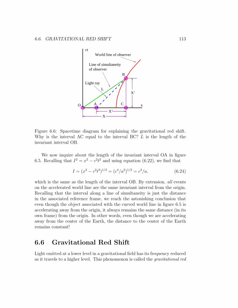
6.6. GRAVITATIONAL RED SHIFT 113
ct
x
X’
B
A
X’X
O
Light ray
World line of observer
Line of simultaneityof observer
C
L
Figure 6.6: Spacetime diagram for explaining the gravitational red shift.Why is the interval AC equal to the interval BC? L is the length of theinvariant interval OB.
We now inquire about the length of the invariant interval OA in figure6.5. Recalling that I2 = x2 − c2t2 and using equation (6.22), we find that
I = (x2 − c2t2)1/2 = (c4/a2)1/2 = c2/a, (6.24)
which is the same as the length of the interval OB. By extension, all eventson the accelerated world line are the same invariant interval from the origin.Recalling that the interval along a line of simultaneity is just the distancein the associated reference frame, we reach the astonishing conclusion thateven though the object associated with the curved world line in figure 6.5 isaccelerating away from the origin, it always remains the same distance (in itsown frame) from the origin. In other words, even though we are acceleratingaway from the center of the Earth, the distance to the center of the Earthremains constant!
6.6 Gravitational Red Shift
Light emitted at a lower level in a gravitational field has its frequency reducedas it travels to a higher level. This phenomenon is called the gravitational red

114 CHAPTER 6. ACCELERATION AND GENERAL RELATIVITY
shift. Figure 6.6 shows why this happens. Since experiencing a gravitationalforce is equivalent to being in an accelerated reference frame, we can use thetools of special relativity to view the process of light emission and absorptionfrom the point of view of the unaccelerated or inertial frame. In this referenceframe the observer of the light is accelerating to the right, as indicated by thecurved world line in figure 6.6, which is equivalent to a gravitational force tothe left. The light is emitted at point A with frequency ω by a source whichis stationary at this instant. At this instant the observer is also stationary inthis frame. However, by the time the light gets to the observer, he or she hasa velocity to the right which means that the observer measures a Dopplershifted freqency ω′ for the light. Since the observer is moving away from thesource, ω′ < ω, as indicated above.
The relativistic Doppler shift is given by
ω′
ω=
(
1 − U/c
1 + U/c
)1/2
, (6.25)
so we need to compute U/c. The line of simultaneity for the observer at pointB goes through the origin, and is thus given by line segment OB in figure 6.6.The slope of this line is U/c, where U is the velocity of the observer at pointB. From the figure we see that this slope is also given by the ratio X ′/X.Equating these, eliminating X in favor of L = (X2 − X ′2)1/2, which is theactual invariant distance of the observer from the origin, and substitutinginto equation (6.25) results in our gravitational red shift formula:
ω′
ω=
(
X −X ′
X +X ′
)1/2
=
(
(L2 +X ′2)1/2 −X ′
(L2 +X ′2)1/2 +X ′
)1/2
. (6.26)
If X ′ = 0, then there is no redshift, because the source is collocated with theobserver. On the other hand, if the source is located at the origin, so X ′ = X,the Doppler shifted frequency is zero. In addition, the light never gets to theobserver, since the world line is asymptotic to the light world line passingthrough the origin. If the source is at a higher level in the gravitational fieldthan the observer, so that X ′ < 0, then the frequency is shifted to a highervalue, i. e., it becomes a “blue shift”.

6.7. EVENT HORIZONS 115
x
t
A B
E
F
CD
Figure 6.7: Position of an object as a function of time.
6.7 Event Horizons
The 45◦ diagonal line passing through the origin in figure 6.5 is called theevent horizon for the accelerated observer in this figure. Notice that lightfrom the “twilight zone” above and to the left of the event horizon cannotreach the accelerated observer. However, the reverse is not true — a lightsignal emitted to the left by the observer can cross the event horizon into the“twilight zone”. The event horizon thus has a peculiar one-way character —it passes signals from right to left, but not from left to right.
6.8 Problems
1. An object moves as described in figure 6.7, which shows its position xas a function of time t.
(a) Is the velocity positive, negative, or zero at each of the points A,B, C, D, E, and F?
(b) Is the acceleration positive, negative, or zero at each of the pointsA, B, C, D, E, and F?
2. An object is moving counterclockwise at constant speed around thecircle shown in figure 6.8 due to the fact that it is attached by a stringto the center of the circle at point O.
(a) Sketch the object’s velocity vectors at points A, B, and C.

116 CHAPTER 6. ACCELERATION AND GENERAL RELATIVITY
O
C
B
A
Figure 6.8: Object in circular motion.
(b) Sketch the object’s acceleration vectors at points A, B, and C.
(c) If the string breaks at point A, sketch the subsequent trajectoryfollowed by the object.
3. How fast are you going after accelerating from rest at a = 10 m s−2 for
(a) 10 y?
(b) 100000 y?
Express your answer as the speed of light minus your actual speed.Hint: You may have a numerical problem on the second part, whichyou should try to resolve using the approximation (1 + ǫ)x ≈ 1 + xǫ,which is valid for |ǫ| ≪ 1.
4. An object’s world line is defined by x(t) = (d2 + c2t2)1/2 where d is aconstant and c is the speed of light.
(a) Find the object’s velocity as a function of time.
(b) Using the above result, find the slope of the tangent to the worldline as a function of time.
(c) Find where the line of simultaneity corresponding to each tangentworld line crosses the x axis.
5. A car accelerates in the positive x direction at 3 m s−2.
(a) What is the net force on a 100 kg man in the car as viewed froman inertial reference frame?

6.8. PROBLEMS 117
(b) What is the inertial force experienced by this man in the referenceframe of the car?
(c) What is the net force experienced by the man in the car’s (accel-erated) reference frame?
6. A person is sitting in a comfortable chair in her home in Bogota,Columbia, which is essentially on the equator.
(a) What would the rotational period of the earth have to be to makethis person weightless?
(b) What is her acceleration according to the equivalence principle inthis situation?
7. At time t = 0 a Zork (a creature from the planet Zorkheim) acceler-ating to the right at a = 103 m s−2 in a spaceship accidently drops itsstopwatch off of the spaceship.
(a) Describe qualitatively how the hands of the watch appear to moveto the Zork as it observes the watch through a powerful telescope.
(b) After a very long time what does the watch read?
Hint: Draw a spacetime diagram with the world lines of the spaceshipand the watch. Then send light rays from the watch to the spaceship.
8. Using a spacetime diagram, show why signals from events on the hiddenside of the event horizon from an accelerating spaceship cannot reachthe spaceship.

118 CHAPTER 6. ACCELERATION AND GENERAL RELATIVITY

Chapter 7
Matter Waves
We begin our study of quantum mechanics by discussing the diffraction un-dergone by X-rays and electrons when they interact with a crystal. X-raysare a form of electromagnetic radiation with wavelengths comparable to thedistances between atoms. Scattering from atoms in a regular crystallinestructure results in an interference pattern which is in many ways similarto the pattern from a diffraction grating. We first develop Bragg’s law fordiffraction of X-rays from a crystal. Two practical techniques for doing X-raydiffraction are then described.
It turns out that electrons have wave-like properties and also undergoBragg diffraction by crystals. Bragg diffraction thus provides a crucial bridgebetween the worlds of waves and particles. With this bridge we introducethe classical ideas of momentum and energy by relating them to the wavevector and frequency of a wave. The properties of waves also give rise to theHeisenberg uncertainty principle.
Table 7.1 shows a table of the Nobel prizes associated with the ideaspresented in this chapter. This gives us a feel for the chronology of thesediscoveries and indicates how important they were to the development ofphysics in the early 20th century.
7.1 Bragg’s Law
Figure 7.1 schematically illustrates interference between waves scatteringfrom two adjacent rows of atoms in a crystal. The net effect of scatteringfrom a single row is equivalent to partial reflection from a mirror imagined to
119

120 CHAPTER 7. MATTER WAVES
Year Recipient Contribution
1901 W. K. Rontgen Discovery of X-rays1906 J. J. Thomson Discovery of electron1914 M. von Laue X-ray diffraction in crystals1915 W. and L. Bragg X-ray analysis of crystal structure1918 M. Planck Energy quantization1921 A. Einstein Photoelectric effect1922 N. Bohr Structure of atoms1929 L.-V. de Broglie Wave nature of electrons1932 W. Heisenberg Quantum mechanics1933 Schrodinger and Dirac Atomic theory1937 Davisson and Thomson Electron diffraction in crystals
Table 7.1: Selected Nobel prize winners, year of award, and contribution.
d
θ
θ
h
Figure 7.1: Schematic diagram for determining Bragg’s law.

7.2. X-RAY DIFFRACTION TECHNIQUES 121
be aligned with the row. Thus, the angle of “reflection” equals the angle ofincidence for each row. Interference then occurs between the beams reflectingoff different rows of atoms in the crystal.
For the two adjacent rows shown in figure 7.1, the path difference be-tween beams is 2h = 2d sin θ. For constructive interference this must be aninteger number of wavelengths, mλ, where the integer m is called the order
of interference. The result is Bragg’s law of diffraction:
mλ = 2d sin θ, m = 1, 2, 3 . . . (Bragg’s law). (7.1)
If only two rows are involved, the transition from constructive to destruc-tive interference as θ changes is gradual. However, if interference from manyrows occurs, then the constructive interference peaks become very sharp withmostly destructive interference in between. This sharpening of the peaks asthe number of rows increases is very similar to the sharpening of the diffrac-tion peaks from a diffraction grating as the number of slits increases.
7.2 X-Ray Diffraction Techniques
Two types of targets are used in Bragg diffraction experiments, single crystalsand powder targets.
7.2.1 Single Crystal
In a single crystal setup, an X-ray detector is mounted as shown in figure7.2. A mechanical device keeps the detector oriented so that the angle ofincidence equals the angle of reflection for the desired crystal plane. Peaksin the X-ray detection rate are sought as the angle θ is varied.
The advantage of this type of apparatus is that diffraction peaks fromonly the selected crystal plane are observed.
7.2.2 Powder Target
The powder in a powder target is really a conglomeration of many tiny crys-tals randomly oriented. Thus, for each possible Bragg diffraction angle thereare crystals oriented correctly for Bragg diffraction to take place. The de-tector is usually a photographic plate or an equivalent electronic device as

122 CHAPTER 7. MATTER WAVES
θ2θ
single crystalsourceX-ray
X-ray detectorcrystal plane
Figure 7.2: Setup for single crystal Bragg diffraction.
end view
sourceX-ray
powder target
side view
Figure 7.3: Setup for powder target Bragg diffraction.

7.3. MEANING OF QUANTUM WAVE FUNCTION 123
illustrated in figure 7.3. For each Bragg diffraction angle one sees a ring onthe plate concentric with the axis of the incident X-ray beam.
The advantage of this type of system is that no a priori knowledge isneeded of the crystal plane orientations. Furthermore, a single large crystalis not required. However, all possible Bragg scattering angles are seen atonce, which can lead to confusion in the interpretation of the results.
7.3 Meaning of Quantum Wave Function
Bragg diffraction illustrates the most difficult thing to understand aboutquantum mechanics, namely that particles can have wave-like properties andwaves can have particle-like properties.
The variation of X-ray intensity with angle seen in a Bragg diffraction ap-paratus is very difficult to explain in any terms other than wave interference.Yet, X-rays are typically detected by a device such as a Geiger counter whichproduces a pulse of electricity for each X-ray particle, or photon, which hitsit. Thus, X-rays sometimes act like particles and sometimes like waves.
Light isn’t alone in having both particle and wave properties. Davissonand Germer and later G. P. Thomson (son of J. J. Thomson, the discovererof the electron) showed that electrons also can act like waves. They did thisby demonstrating that electrons undergo Bragg diffraction in crystals, muchas X-rays do.
Most physicists (including Albert Einstein) have found quantum mechan-ics to be extremely bizarre, so if you feel the same way, you are in good com-pany! However, there is a useful interpretation of quantum mechanics whichat least allows us to get on with using it to solve problems, even though itmay not satisfy our intuitive reservations about the theory.
The displacement of a quantum mechanical wave associated with a par-ticle is usually called the wave function, ψ. Like light, it is not at all clearwhat ψ is a displacement of, but its use is straightforward. The absolutesquare of the wave function, |ψ(x, t)|2, is proportional to the probability offinding the associated particle at position x and time t. The absolute squareis taken because under many circumstances the wave function is actuallycomplex, i. e., it has both real and imaginary parts. The reasons for this willbe discussed later.
Due to the interpretation of the wave function, quantum mechanics isa probabilistic theory. It does not tell us with certainty what happens to

124 CHAPTER 7. MATTER WAVES
a particular particle. Instead, it tells us, for instance, the probabilities forthe particle to be detected in certain locations. If many experiments aredone, with one particle per experiment, the numbers of experiments withparticles being detected in the various possible locations are in proportion tothe quantum mechanical probabilities.
7.4 Sense and Nonsense in Quantum Mechan-
ics
The essential mystery of quantum mechanics becomes clearer when discussedin the conceptually simpler context of two slit interference. If light andelectrons can have both particle and wave properties, then one might askthrough which of the two slits the particle passed. However, in physics aquestion simply doesn’t make sense if it cannot be answered by experiment.Let us see if the above question makes sense.
One can indeed perform an experiment to determine which slit the X-rayphoton or electron passes through in the two slit experiment. However, by
the very act of making this measurement, the form of the associated waveis altered. In particular, since the absolute square of the wave displacementrepresents the probability of finding the particle, once the particle has def-initely been found passing through one or the other of the slits, the wavefunction collapses into a very small wave packet located at the observed po-sition of the particle. Thus, the wave displacement becomes zero at the slitit didn’t pass through. However, the interference pattern results from thesuperposition of waves emanating from two slits. If no wave comes from oneof the slits (because the wave displacement is zero there), then there can beno interference pattern!
We can now make the inverse argument. If there is an interference pat-tern, then we know that the wave displacement is non-zero at both slits.From the probability interpretation of the wave displacement, we concludethat we cannot say, even in principle, through which slit the particle passed.It is not just that we don’t know the answer to this question; there is simply
no experiment which can give us an answer without destroying the interfer-ence pattern. In other words, the question “Which slit did the particle passthrough?” is a nonsensical question in the case where an interference patternis actually produced.

7.4. SENSE AND NONSENSE IN QUANTUM MECHANICS 125
The American physicist Richard Feynman noticed that the above behav-ior can be interpreted as violating the normal laws of probability. These lawssay that the probability of an event is the sum of the probabilities of alternateindependent ways for that event to occur. For instance, the probability for aparticle to reach point A on the detection screen of a two slit setup is just theprobability P1 for the particle to reach point A after going through slit 1, plusthe probability P2 for the particle to reach point A after going through slit 2.Thus, if P1 = P2 = 0.1, then the probability for the particle to reach pointA irrespective of which slit it went through should be Ptotal = P1 +P2 = 0.2.However, if point A happens to be a point of destructive interference, thenwe know that Ptotal = 0.
Feynman proposed that the above rule stating that alternate independentprobabilities add, is simply incorrect. In its place Feynman asserted thatprobability amplitudes add instead, where the probability amplitude in thiscase is just the wave function associated with the particle. The probability isobtained by adding the alternate probability amplitudes together and takingthe absolute square of the sum.
In the two slit case, let us call ψ1 the amplitude for the particle to reachpoint A via slit 1, while ψ2 is the amplitude for it to reach this point via slit 2.The total amplitude is therefore ψtotal = ψ1 + ψ2 and the overall probabilityfor the particle to reach point A is Ptotal = |ψ1 + ψ2|
2. The wave functionsψ1 and ψ2 at point A are proportional respectively to sin(kL1) and sin(kL2),where k is the wavenumber and L1 and L2 are the respective distances fromslit 1 and slit 2 to point A. It is easy to see that destructive interferenceoccurs if the difference between L1 and L2 is half a wavelength, thus yieldingPtotal = 0.
The above treatment of two slits in terms of probability amplitudes yieldsresults which are identical to the conventional treatment of the two slit prob-lem for waves. However, it is conceptually clearer in the case of quantummechanics because we no longer need to ask whether “things” are really par-ticles or waves. In particular, the particle/wave is replaced by just a particleplus the assertion that probability amplitudes rather than probabilities add.The laws of quantum mechanics then boil down to rules for how probabil-ity amplitudes behave. In the case of particles, the amplitudes behave likewaves, which explains why the study of wave kinematics and dynamics is soimportant to our understanding of quantum mechanics.

126 CHAPTER 7. MATTER WAVES
7.5 Mass, Momentum, and Energy
In this section we relate the classical ideas of mass, momentum and energyto what we have done so far. Historically, these connections were first madeby Max Planck and Louis de Broglie with help from Albert Einstein. Braggdiffraction by electrons is invoked as an experimental test of the Planck andde Broglie relations.
Technically, we don’t need the ideas of mass, momentum, and energy todo physics – the notions of wavenumber, frequency, and group velocity aresufficient to describe and explain all observed phenomena. However, mass,momentum, and energy are so firmly embedded in physics that one couldn’ttalk to other physicists without an understanding of these quantities!
7.5.1 Planck, Einstein, and de Broglie
Max Planck was the first to make a connection between the energy of aparticle and the frequency of the associated wave. Planck developed hisformula in his successful attempt to explain the emission and absorptionof electromagnetic radiation from warm material surfaces. It suffices hereto convey Planck’s formula, which was originally intended to apply only toparcels of electromagnetic radiation, or photons:
E = hf = hω (Planck relation), (7.2)
where E is the energy of the photon, f is the rotational frequency of theassociated light wave, and ω is its angular frequency. The constant h =6.63 × 10⁻³⁴ kg m2 s−1 is called Planck’s constant. The related constanth = h/2π = 1.06 × 10⁻³⁴ kg m2 s−1 is also referred to as Planck’s constant,but to avoid confusion with the original constant, we will generally refer toit as “h bar”.
Notice that a new physical dimension has appeared, namely mass, withthe unit kilogram, abbreviated “kg”. The physical meaning of mass is muchlike our intuitive understanding of the concept, i. e., as a measure of theresistance of an object to its velocity being changed. The precise scientificmeaning will emerge shortly.
Einstein showed that Planck’s idea could be used to explain the emissionof electrons which occurs when light impinges on the surface of a metal.This emission, which is called the photoelectric effect, can only occur whenelectrons are supplied with a certain minimum energy EB required to break

7.5. MASS, MOMENTUM, AND ENERGY 127
them loose from the metal. Experiment shows that this emission occurs onlywhen the frequency of the light exceeds a certain minimum value. This valueturns out to equal ωmin = EB/h, which suggests that electrons gain energyby absorbing a single photon. If the photon energy, hω, exceeds EB, thenelectrons are emitted, otherwise they are not. It is much more difficult toexplain the photoelectric effect from the classical theory of light.
Louis de Broglie proposed that Planck’s energy-frequency relationshipbe extended to all kinds of particles. In addition he hypothesized that themomentum Π of the particle and the wave vector k of the correspondingwave were similarly related:
Π = hk (de Broglie relation). (7.3)
Note that this can also be written in scalar form in terms of the wavelengthas Π = h/λ.
De Broglie’s hypothesis was inspired by the fact that wave frequency andwavenumber are components of the same four-vector according to the theoryof relativity, and are therefore closely related to each other. Thus, if the en-ergy of a particle is related to the frequency of the corresponding wave, thenthere ought to be some similar quantity which is correspondingly related tothe wavenumber. It turns out that the momentum is the appropriate quan-tity. The physical meaning of momentum will become clear as we proceed.
We will also find that the rest frequency, µ, of a particle is related to itsmass, m:
Erest ≡ mc2 = hµ. (7.4)
The quantity Erest is called the rest energy of the particle.From our perspective, energy, momentum, and rest energy are just scaled
versions of frequency, wave vector, and rest frequency, with a scaling factorh. We can therefore define a four-momentum as a scaled version of the wavefour-vector:
Π = hk. (7.5)
The spacelike component of Π is just Π, while the timelike part is E/c.Planck, Einstein, and de Broglie had extensive backgrounds in classical
mechanics, in which the concepts of energy, momentum, and mass have pre-cise meaning. In this text we do not presuppose such a background. Perhapsthe best strategy at this point is to think of these quantities as scaled ver-sions of frequency, wavenumber, and rest frequency, where the scale factor is

128 CHAPTER 7. MATTER WAVES
h. The significance of these quantities to classical mechanics will emerge bitby bit.
7.5.2 Wave and Particle Quantities
Let us now recapitulate what we know about relativistic waves, and how thisknowledge translates into knowledge about the mass, energy, and momentumof particles. In the following equations, the left form is expressed in waveterms, i. e., in terms of frequency, wavenumber, and rest frequency. Theright form is the identical equation expressed in terms of energy, momentum,and mass. Since the latter variables are just scaled forms of the former, thetwo forms of each equation are equivalent.
We begin with the dispersion relation for relativistic waves:
ω2 = k2c2 + µ2 E2 = Π2c2 +m2c4. (7.6)
Calculation of the group velocity, ug = dω/dk, from the dispersion relationyields
ug =c2k
ωug =
c2Π
E. (7.7)
These two sets of equations represent what we know about relativistic waves,and what this knowledge tells us about the relationships between the mass,energy, and momentum of relativistic particles. When in doubt, refer back
to these equations, as they work in all cases, including for particles with zero
mass!
It is useful to turn equations (7.6) and (7.7) around so as to express thefrequency as a function of rest frequency and group velocity,
ω =µ
(1 − u2g/c
2)1/2E =
mc2
(1 − u2g/c
2)1/2, (7.8)
and the wavenumber as a similar function of these quantities:
k =µug/c
2
(1 − u2g/c
2)1/2Π =
mug
(1 − u2g/c
2)1/2. (7.9)
Note that equations (7.8) and (7.9) work only for particles with non-zero
mass! For zero mass particles you need to use equations (7.6) and (7.7) withm = 0 and µ = 0.

7.5. MASS, MOMENTUM, AND ENERGY 129
The quantity ω − µ indicates how much the frequency exceeds the restfrequency. Notice that if ω = µ, then from equation (7.6) k = 0. Thus,positive values of ωk ≡ ω−µ indicate |k| > 0, which means that the particleis moving according to equation (7.7). Let us call ωk the kinetic frequency :
ωk =
[
1
(1 − u2g/c
2)1/2− 1
]
µ K =
[
1
(1 − u2g/c
2)1/2− 1
]
mc2. (7.10)
We call K the kinetic energy for similar reasons. Again, equation (7.10) only
works for particles with non-zero mass. For zero mass particles the kineticenergy equals the total energy.
7.5.3 Non-Relativistic Limits
When the mass is non-zero and the group velocity is much less than the speedof light, it is useful to compute approximate forms of the above equationsvalid in this limit. Using the approximation (1 + ǫ)x ≈ 1 + xǫ, we find thatthe dispersion relation becomes
ω = µ+k2c2
2µE = mc2 +
Π2
2m, (7.11)
and the group velocity equation takes the approximate form
ug =c2k
µug =
Π
m. (7.12)
The non-relativistic limits for equations (7.8) and (7.9) become
ω = µ+µu2
g
2c2E = mc2 +
mu2g
2(7.13)
andk = µug/c
2 Π = mug, (7.14)
while the approximate kinetic energy equation is
ωk =µu2
g
2c2K =
mu2g
2. (7.15)
Just a reminder — the equations in this section are not valid for massless
particles!
130 CHAPTER 7. MATTER WAVES
7.5.4 An Experimental Test
How can we test the above predictions against experiment? The key pointis to be able to relate the wave aspects to the particle aspects of a quantummechanical wave-particle. Equation (7.9), or equation (7.14) in the non-relativistic case, relates a particle’s wavenumber k to it’s velocity ug. Bothof these quantities can be measured in a Bragg’s law experiment with elec-trons. In this experiment electrons are fired at a crystal with known atomicdimensions at a known speed, which we identify with the group velocityug. The Bragg angle which yields constructive interference can be used tocalculate the wavelength of the corresponding electron wave, and hence thewavenumber and momentum. If the momentum is plotted against group ve-locity in the non-relativistic case, a straight line should be found, the slopeof which is the particle’s mass. In the fully relativistic case one needs toplot momentum versus ug/(1 − u2
g/c2)1/2. Again, a straight line indicates
agreement with the theory and the slope of the line is the particle’s mass.
7.6 Heisenberg Uncertainty Principle
Classically, we consider the location of a particle to be a knowable piece ofinformation. In quantum mechanics the position of a particle is well knownif the wave packet representing it is small in size. However, quantum me-chanics imposes a price on accurately knowing the position of a particle interms of the future predictability of its position. This is because a smallwave packet, which corresponds to accurate knowledge of the correspondingparticle’s position, implies the superposition of plane waves corresponding toa broad distribution of wavenumbers. This translates into a large uncertaintyin the wavenumber, and hence the momentum of the particle. In contrast, abroad wave packet corresponds to a narrower distribution of wavenumbers,and correspondingly less uncertainty in the momentum.
Referring back to chapters 1 and 2, recall that both the longitudinal(along the direction of motion) and transverse (normal to the direction ofmotion) dimensions of a wave packet, ∆xL and ∆xT , can be related to thespread of longitudinal and transverse wavenumbers, ∆kL and ∆kT :
∆kL∆xL ≈ 1, (7.16)
∆kT ∆xT ≈ 1. (7.17)

7.6. HEISENBERG UNCERTAINTY PRINCIPLE 131
We have omitted numerical constants which are order unity in these approx-imate relations so as to show their essential similarity.
The above equations can be interpreted in the following way. Since theabsolute square of the wave function represents the probability of finding aparticle, ∆xL and ∆xT represent the uncertainty in the particle’s position.Similarly, ∆kL and ∆kT represent the uncertainty in the particle’s longitudi-nal and transverse wave vector components. This latter uncertainty leads touncertainty in the particle’s future evolution — larger or smaller longitudinalk results respectively in larger or smaller particle speed, while uncertainty inthe transverse wavenumber results in uncertainty in the particle’s directionof motion. Thus uncertainties in any component of k result in uncertaintiesin the corresponding component of the particle’s velocity, and hence in itsfuture position.
The equations (7.16) and (7.17) show that uncertainty in the present andfuture positions of a particle are complimentary. If the present position isaccurately known due to the small size of the associated wave packet, thenthe future position is not very predictable, because the wave packet dispersesrapidly. On the other hand, a broad-scale initial wave packet means that thepresent position is poorly known, but the uncertainty in position, poor asit is, doesn’t rapidly increase with time, since the wave packet has a smalluncertainty in wave vector and thus disperses slowly. This is a statement ofthe Heisenberg uncertainty principle.
The uncertainty principle also applies between frequency and time:
∆ω∆t ≈ 1. (7.18)
This shows up in the beat frequency equation 1/Tbeat = ∆f = ∆ω/2π. Thebeat period Tbeat may be thought of as the size of a “wave packet in time”.The beat frequency equation may be rewritten as ∆ωTbeat = 2π, which is thesame as equation (7.18) if the factor of 2π is ignored and Tbeat is identifiedwith ∆t.
The above forms of the uncertainty principle are not relativistically in-variant. A useful invariant form may be obtained by transforming to thecoordinate system in which a particle is stationary. In this reference framethe time t becomes the proper time τ associated with the particle. Fur-thermore, the frequency ω becomes the rest frequency µ. The uncertaintyprinciple thus becomes
∆µ∆τ ≈ 1 (7.19)

132 CHAPTER 7. MATTER WAVES
in this reference frame. However, since ∆µ and ∆τ are relativistic invariants,this expression of the uncertainty principle is valid in any reference frame.
It is more common to express the uncertainty principle in terms of themass, momentum, and energy by multiplying equations (7.16) - (7.19) by h.Lumping the momentum equations, we find
∆Π∆x ≈ h, (7.20)
∆E∆t ≈ h, (7.21)
and∆(mc2)∆τ ≈ h. (7.22)
Classical mechanics is the realm of quantum mechanics in which the di-mensions of the system of interest are much larger than the wavelengths ofthe waves corresponding to the particles constituting the system. In thiscase the uncertainties induced by the uncertainty principle are unimportant.This limit is analogous to the geometrical optics limit for light. Thus, wecan say that classical mechanics is the geometrical optics limit of quantummechanics.
7.7 Problems
1. An electron with wavelength λ = 1.2×10⁻¹⁰ m undergoes Bragg diffrac-tion from a single crystal with atomic plane spacing of d = 2×10⁻¹⁰ m.
(a) Calculate the Bragg angles (all of them!) for which constructiveinterference occurs.
(b) Calculate the speed of the electron.
2. Suppose that electrons impinge on two slits in a plate, resulting in atwo slit diffraction pattern on a screen on the other side of the plate.The amplitude for an electron to pass through either one of the slitsand reach point A on the screen is ψ. Thus, the probability for anelectron to reach this point is |ψ|2 if there is only a single slit open.
(a) If there are two slits open and A is a point of constructive inter-ference, what is the probability of an electron reaching A?
(b) If there are two slits open and A is a point of destructive interfer-ence, what is the probability of an electron reaching A?

7.7. PROBLEMS 133
(c) If there are two slits open, what is the probability for an electron toreach point A according to the conventional rule that probabilitiesadd? (This is the result one would expect if, for instance, theparticles were machine gun bullets and the slits were, say, 5 cmapart.)
(d) If the slit separation is very much greater than the electron wave-length, how does this affect the spacing of regions of constructiveand destructive interference? Explain how the results of parts (a)and (b) become approximately consistent with those of part (c)in this case.
3. Compute the (angular) rest frequency of an electron and a neutron.(Look up their masses.)
4. How does the dispersion relation for relativistic waves simplify if therest frequency (and hence the particle mass) is zero? What is the groupvelocity in this case?
5. X-rays are photons with frequencies about 2000 times the frequen-cies of ordinary light photons. From this information and what youknow about light, infer the approximate velocity of electrons whichhave Bragg diffraction properties similar to X-rays. Are the electronsrelativistic or non-relativistic?
6. Electrons with velocity v = 0.6c are diffracted with a 0.2 radian half-angle of diffraction when they hit an object. What is the approximatesize of the object? Hint: Diffraction of a wave by an object of a certainsize is quite similar to diffraction by a hole in a screen of the same size.
7. Work out an approximate formula for the kinetic energy of a particle asa function of mass m and velocity ug which is valid when u2
g ≪ c2. Hint:Use the approximation (1 + ǫ)x ≈ 1 + xǫ, which is valid for |ǫ| ≪ 1. Asug/c becomes larger, how does this approximate formula deviate fromthe exact formula?
8. Work out an approximate formula for the momentum of a particle asa function of m and ug in the case where u2
g ≪ c2. You may wish touse the approximation mentioned in the previous problem.

134 CHAPTER 7. MATTER WAVES
9. If a photon is localized to within a distance ∆x, what is the uncertaintyin the photon energy?
10. If an electron is localized to within a distance ∆x, what is the un-certainty in the electron kinetic energy? Hint: As long as ∆Π ≪ Π,∆Π2 ≈ 2Π∆Π. To see why, compute dΠ2/dΠ.
11. A grocer dumps some pinto beans onto a scale, estimates their massas 2 kg, and then dumps them off after 5 s. What is the quantummechanical uncertainty in this measurement? For this problem only,assume that the speed of light is 10 m s−1 (speed of a fast buggy) andthat h = 1 kg m2 s−1.
12. Mary’s physics text (mass 0.3 kg) has to be kept on a leash (length0.5 m) to prevent it from wandering away from her in Quantum World(h = 1 kg m2 s−1).
(a) If the leash suddenly breaks, what is the maximum speed at whichthe book is likely to move away from its initial location?
(b) In order to reduce this speed, should Mary make the new leashshorter or longer than the old one? Explain.
13. A proton (mass M = 1.7 × 10⁻²⁷ kg) is confined to an atomic nucleusof diameter D = 2 × 10⁻¹⁵ m.
(a) What is the uncertainty in the proton’s momentum?
(b) Roughly what kinetic energy might you expect the proton to have?
Planck’s constant is h = 1.06 × 10⁻³⁴ kg m2 s−1. You may use thenon-relativistic equation for the energy.

Chapter 8
Geometrical Optics and
Newton’s Laws
The question that motivates us to study physics is “What makes things go?”The answers we conceive to this question constitute the subject of dynamics.This is in contrast to the question we have primarily addressed so far, namely“How do things go?” As noted earlier, the latter question is about kinematics.Extensive preparation in the kinematics of waves and particles in relativisticspacetime is needed to intelligently address dynamics. This preparation isnow complete.
In this chapter we outline three different dynamical principles based re-spectively on pre-Newtonian, Newtonian, and quantum mechanical thinking.We first discuss the Newtonian mechanics of conservative forces in one di-mension. Certain ancillary concepts in mechanics such as work and powerare introduced at this stage. We then show that Newtonian and quantummechanics are consistent with each other in the realm in which they overlap,i. e., in the geometrical optics limit of quantum mechanics. For simplicity,this relationship is first developed in one dimension in the non-relativisticlimit. Higher dimensions require the introduction of partial derivatives, andthe relativistic case will be considered later.
8.1 Fundamental Principles of Dynamics
Roughly speaking, there have been three eras of physics, characterized bythree different answers to the question of what makes things go.
135

136 CHAPTER 8. GEOMETRICAL OPTICS AND NEWTON’S LAWS
8.1.1 Pre-Newtonian Dynamics
Aristotle expounded a view of dynamics which agrees closely with our every-day experience of the world. Objects only move when a force is exerted uponthem. As soon as the force goes away, the object stops moving. The act ofpushing a box across the floor illustrates this principle — the box certainlydoesn’t move by itself!
8.1.2 Newtonian Dynamics
In contrast to earthly behavior, the motions of celestial objects seem effort-less. No obvious forces act to keep the planets in motion around the sun. Infact, it appears that celestial objects simply coast along at constant velocityunless something acts on them. The Newtonian view of dynamics — objectschange their velocity rather than their position when a force is exerted onthem — is expressed by Newton’s second law :
F = ma (Newton’s second law), (8.1)
where F is the force exerted on a body, m is its mass, and a is its acceleration.Newton’s first law, which states that an object remains at rest or in uniformmotion unless a force acts on it, is actually a special case of Newton’s secondlaw which applies when F = 0.
It is no wonder that the first successes of Newtonian mechanics were inthe celestial realm, namely in the predictions of planetary orbits. It tookNewton’s genius to realize that the same principles which guided the planetsalso applied to the earthly realm as well. In the Newtonian view, the tendencyof objects to stop when we stop pushing on them is simply a consequence offrictional forces opposing the motion. Friction, which is so important on theearth, is negligible for planetary motions, which is why Newtonian dynamicsis more obviously valid for celestial bodies.
Note that the principle of relativity is closely related to Newtonian physicsand is incompatible with pre-Newtonian views. After all, two referenceframes moving relative to each other cannot be equivalent in the pre-Newtonianview, because objects with nothing pushing on them can only come to restin one of the two reference frames!
Einstein’s relativity is often viewed as a repudiation of Newton, but thisis far from the truth — Newtonian physics makes the theory of relativitypossible through its invention of the principle of relativity. Compared with

8.2. POTENTIAL ENERGY 137
the differences between pre-Newtonian and Newtonian dynamics, the changesneeded to go from Newtonian to Einsteinian physics constitute minor tinker-ing.
8.1.3 Quantum Dynamics
In quantum mechanics, particles are represented by matter waves, with theabsolute square of the wave displacement yielding the probability of find-ing the particle. The behavior of particles thus follows from the reflection,refraction, diffraction, and interference of the associated waves. The connec-tion with Newtonian dynamics comes from tracing the trajectories of matterwave packets. Changes in the speed and direction of motion of these packetscorrespond to the accelerations of classical mechanics. When wavelengthsare small compared to the natural length scale of the problem at hand, thewave packets can be made small, thus pinpointing the position of the as-sociated particle, without generating excessive uncertainty in the particle’smomentum. This is the geometrical optics limit of quantum mechanics.
8.2 Potential Energy
We now address Newtonian mechanics in the case where the force on a par-ticle is conservative. A conservative force is one that can be derived from aso-called potential energy U . We assume that the potential energy of the par-ticle depends only on its position. The force is obtained from the potentialenergy by the equation
F = −dU
dx. (8.2)
Using this equation we write Newton’s second law as
−dU
dx= ma. (8.3)
We then notice that the acceleration can be written in terms of the x deriva-tive of v2/2:
a =dv
dt=dv
dx
dx
dt=dv
dxv =
1
2
dv2
dx. (8.4)
The last step in the above derivation can be verified by applying the prod-uct rule: dv2/dt = d(vv)/dt = v(dv/dt) + (dv/dt)v = 2v(dv/dt). Putting
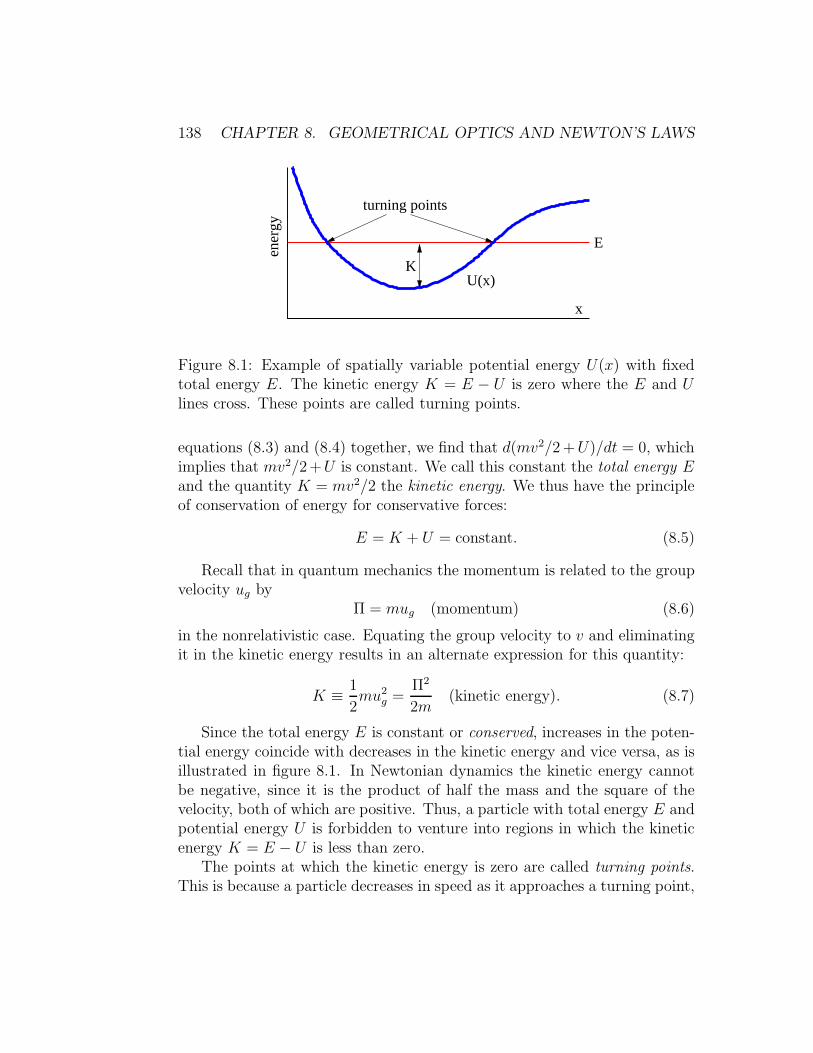
138 CHAPTER 8. GEOMETRICAL OPTICS AND NEWTON’S LAWS
x
ener
gy
E
K
turning points
U(x)
Figure 8.1: Example of spatially variable potential energy U(x) with fixedtotal energy E. The kinetic energy K = E − U is zero where the E and Ulines cross. These points are called turning points.
equations (8.3) and (8.4) together, we find that d(mv2/2 +U)/dt = 0, whichimplies that mv2/2+U is constant. We call this constant the total energy Eand the quantity K = mv2/2 the kinetic energy. We thus have the principleof conservation of energy for conservative forces:
E = K + U = constant. (8.5)
Recall that in quantum mechanics the momentum is related to the groupvelocity ug by
Π = mug (momentum) (8.6)
in the nonrelativistic case. Equating the group velocity to v and eliminatingit in the kinetic energy results in an alternate expression for this quantity:
K ≡1
2mu2
g =Π2
2m(kinetic energy). (8.7)
Since the total energy E is constant or conserved, increases in the poten-tial energy coincide with decreases in the kinetic energy and vice versa, as isillustrated in figure 8.1. In Newtonian dynamics the kinetic energy cannotbe negative, since it is the product of half the mass and the square of thevelocity, both of which are positive. Thus, a particle with total energy E andpotential energy U is forbidden to venture into regions in which the kineticenergy K = E − U is less than zero.
The points at which the kinetic energy is zero are called turning points.This is because a particle decreases in speed as it approaches a turning point,

8.3. WORK AND POWER 139
stops there for an instant, and reverses direction. Note also that a particlewith a given total energy always has the same speed at some point x regard-less of whether it approaches this point from the left or the right:
speed = |ug| = | ± [2(E − U)/m]1/2|. (8.8)
8.2.1 Gravity as a Conservative Force
An example of a conservative force is gravity. An object of mass m near thesurface of the earth has the gravitational potential energy
U = mgz (gravity near earth’s surface) (8.9)
where z is the height of the object and g = 9.8 m s−2 is the local value ofthe gravitational field near the earth’s surface. Notice that the gravitationalpotential energy increases upward. The speed of the object in this case is|ug| = [2(E −mgz)/m]1/2. If |ug| is known to equal the constant value u0 atelevation z = 0, then equations (8.8) and (8.9) tell us that u0 = (2E/m)1/2
and |ug| = (u20− 2gz)1/2.
There are certain types of questions which energy conservation cannotdirectly answer. For instance if an object is released at elevation h withzero velocity at t = 0, at what time will it reach z = 0 under the influenceof gravity? In such cases it is often easiest to return to Newton’s secondlaw. Since the force on the object is F = −dU/dz = −mg in this case,we find that the acceleration is a = F/m = −mg/m = −g. However,a = du/dt = d2z/dt2, so
u = −gt+ C1 z = −gt2/2 + C1t+ C2 (constant gravity), (8.10)
where C1 and C2 are constants to be determined by the initial conditions.These results can be verified by differentiating to see if the original acceler-ation is recovered. Since u = 0 and z = h at t = 0, we have C1 = 0 andC2 = h. With these results it is easy to show that the object reaches z = 0when t = (2h/g)1/2.
8.3 Work and Power
When a force is exerted on an object, energy is transferred to the object. Theamount of energy transferred is called the work done on the object. However,

140 CHAPTER 8. GEOMETRICAL OPTICS AND NEWTON’S LAWS
energy is only transferred if the object moves. The work W done is
W = F∆x (8.11)
where the distance moved by the object is ∆x and the force exerted on it isF . Notice that work can either be positive or negative. The work is positiveif the object being acted upon moves in the same direction as the force, withnegative work occurring if the object moves opposite to the force.
Equation (8.11) assumes that the force remains constant over the full dis-placement ∆x. If it is not, then it is necessary to break up the displacementinto a number of smaller displacements, over each of which the force canbe assumed to be constant. The total work is then the sum of the worksassociated with each small displacement.
If more than one force acts on an object, the works due to the differentforces each add or subtract energy, depending on whether they are positiveor negative. The total work is the sum of these individual works.
There are two special cases in which the work done on an object is relatedto other quantities. If F is the total force acting on the object, then W =F∆x = ma∆x by Newton’s second law. However, a = dv/dt where v is thevelocity of the object, and ∆x = (∆x/∆t)∆t ≈ v∆t, where ∆t is the timerequired by the object to move through distance ∆x. The approximationbecomes exact when ∆x and ∆t become very small. Putting all of thistogether results in
Wtotal = mdv
dtv∆t =
d
dt
(
mv2
2
)
∆t = ∆K (total work), (8.12)
where K is the kinetic energy of the object. Thus, when F is the only force,W = Wtotal is the total work on the object, and this equals the change inkinetic energy of the object. This is called the work-energy theorem, and itdemonstrates that work really is a transfer of energy to an object.
The other special case occurs when the force is conservative, but is notnecessarily the total force acting on the object. In this case
Wcons = −dU
dx∆x = −∆U (conservative force), (8.13)
where ∆U is the change in the potential energy of the object associated withthe force of interest.

8.4. MECHANICS AND GEOMETRICAL OPTICS 141
The power associated with a force is simply the amount of work done bythe force divided by the time interval ∆t over which it is done. It is thereforethe energy per unit time transferred to the object by the force of interest.From equation (8.11) we see that the power is
P =F∆x
∆t= Fv (power), (8.14)
where v is the velocity at which the object is moving. The total power is justthe sum of the powers associated with each force. It equals the time rate ofchange of kinetic energy of the object:
Ptotal =Wtotal
∆t=dK
dt(total power). (8.15)
8.4 Mechanics and Geometrical Optics
Louis de Broglie1 made an analogy between matter waves and light waves,pointing out that wave packets of light change their velocity as the resultof spatial variations in the index of refraction of the medium in which theyare travelling. This behavior comes about because the dispersion relationfor light traveling through a medium with index of refraction n is ω = kc/n,so that the group velocity, ug = dω/dk = c/n. Thus, when n increases, ug
decreases, and vice versa.2
In this section we pursue de Broglie’s analogy to see if we can comeup with a theory of matter waves which gives the same results as classicalmechanics in the geometrical optics limit of these waves. We pretend that wedon’t know anything about classical mechanics and make a simple guess as tohow to modify the free particle dispersion relation for matter waves, limitingconsideration initially to the one-dimensional, non-relativistic case. As inmany situations in physics, the simple guess turns out to be correct! Thisleads to a connection between wave dynamics and the Newtonian mechanicsof conservative forces.
1See Louis de Broglie’s 1929 Nobel Prize address, reproduced in Boorse, H. A., and L.Motz, 1966: The World of the Atom, Basic Books.
2This group velocity calculation ignores the possible dependence of index of refractionon wavenumber. If n is a function of k, the calculation is more complicated, but theprinciple is the same.

142 CHAPTER 8. GEOMETRICAL OPTICS AND NEWTON’S LAWS
The dispersion relation for free matter waves is ω = (k2c2 +µ2)1/2. In thenon-relativistic limit k2c2 ≪ µ2 and this equation can be approximated as
ω = µ(1 + k2c2/µ2)1/2 ≈ µ+ k2c2/(2µ). (8.16)
Let us modify this equation by adding a term S ′ which depends on x,and which plays a role analogous to the index of refraction for light:
ω = S ′(x) + µ+ k2c2/(2µ) = S(x) + k2c2/(2µ). (8.17)
The rest frequency has been made to disappear on the right side of the aboveequation by defining S = S ′ + µ. This is done to simplify the notation. Atthis point we don’t know what the physical meaning of S is; we are simplyexploring the consequences of a hunch in the hope that something sensiblecomes out of it.
Let us now imagine that all parts of the wave governed by this dispersionrelation oscillate in phase. The only way this can happen is if ω is constant,i. e., it takes on the same value in all parts of the wave.
If ω is constant, the only way S can vary with x in equation (8.17) is ifthe wavenumber varies in a compensating way. Thus, constant frequency andspatially varying S together imply that k = k(x). Solving equation (8.17)for k yields
k(x) = ±
[
2µ[ω − S(x)]
c2
]1/2
. (8.18)
Since ω is constant, the wavenumber becomes smaller and the wavelengthlarger as the wave moves into a region of increased S.
In the geometrical optics limit, we assume that S doesn’t change muchover one wavelength so that the wave remains reasonably sinusoidal in shapewith approximately constant wavenumber over a few wavelengths. However,over distances of many wavelengths the wavenumber and amplitude of thewave are allowed to vary considerably.
The group velocity calculated from the dispersion relation given by equa-tion (8.17) is
ug =dω
dk=kc2
µ=
(
2c2(ω − S)
µ
)1/2
(8.19)
where k is eliminated in the last step with the help of equation (8.18). Theresulting equation tells us how the group velocity varies as a matter wave

8.5. MATH TUTORIAL – PARTIAL DERIVATIVES 143
traverses a region of slowly varying S. Thus, as S increases, ug decreases andvice versa.
We can now calculate the acceleration of a wave packet resulting fromthe spatial variation in S. We assume that x(t) represents the positionof the wave packet, so that ug = dx/dt. Using the chain rule dug/dt =(dug/dx)(dx/dt) = (dug/dx)ug, we find
a =dug
dt=dug
dxug =
du2g/2
dx= −
c2
µ
dS
dx= −
h
m
dS
dx. (8.20)
The group velocity is eliminated in favor of S by squaring equation (8.19)and substituting the result into equation (8.20).
Comparison of this equation with equation (8.3) solves the mystery as tothe identity of the variable S; it is simply the potential energy divided byPlanck’s constant:
U = hS. (8.21)
Thus, the geometrical optics approach to particle motion is completely equiv-alent to the classical mechanics of a particle moving under the influence of aconservative force, at least in one dimension. We therefore have two ways ofsolving for the motion of a particle subject to a potential energy U(x). Wecan apply the principles of classical mechanics to get the force and the accel-eration of the particle, from which we can derive the motion. Alternatively,we can apply the principles of geometrical optics to compute the spatiallyvariable velocity of the wave packet using equation (8.19). The results arecompletely equivalent, though the methods are conceptually very different.
8.5 Math Tutorial – Partial Derivatives
In order to understand the generalization of Newtonian mechanics to two andthree dimensions, we first need to understand a new type of derivative calledthe partial derivative. The partial derivative is used in functions of more thanone variable. It is just like an ordinary derivative, except that when takingthe derivative of the function with respect to one of the variables, the othervariables are held constant. As an example, let us consider the function
f(x, y) = Ax4 +Bx2y2 + Cy4 (8.22)
144 CHAPTER 8. GEOMETRICAL OPTICS AND NEWTON’S LAWS
where A, B, and C are constants. The partial derivative of f with respectto x is
∂f
∂x= 4Ax3 + 2Bxy2 (8.23)
and the partial derivative with respect to y is
∂f
∂y= 2Bx2y + 4Cy3. (8.24)
That’s it! Note that a special symbol “∂” is used in place of the normal“d” for the partial derivative. This is sometimes called a “curly d”.
8.6 Motion in Two and Three Dimensions
When a matter wave moves through a region of variable potential energy inone dimension, only the wavenumber changes. In two or three dimensions thewave vector can change in both direction and magnitude. This complicatesthe calculation of particle movement. However, we already have an exampleof how to handle this situation, namely, the refraction of light. In that caseSnell’s law tells us how the direction of the wave vector changes, while thedispersion relation combined with the constancy of the frequency gives usinformation about the change in the magnitude of the wave vector. Formatter waves a similar procedure works, though the details are different,because we seek the consequences of a change in potential energy ratherthan a change in the index of refraction.
Figure 8.2 illustrates the refraction of matter waves at a discontinuity inthe potential energy. Let us suppose that the discontinuity occurs at x = 0.If the matter wave to the left of the discontinuity is ψ1 = sin(k1xx+k1yy−ω1t)and to the right is ψ2 = sin(k2xx + k2yy − ω2t), then the wavefronts of thewaves will match across the discontinuity for all time only if ω1 = ω2 ≡ ωand k1y = k2y ≡ ky. We are already familiar with the first condition fromthe one-dimensional problem, so the only new ingredient is the constancy ofthe y component of the wave vector.
In two dimensions the momentum is a vector: Π = mu when |u| ≪ c,where u is the particle velocity. Furthermore, the kinetic energy is K =m|u|2/2 = |Π|2/(2m) = (Π2
x + Π2y)/(2m). The relationship between kinetic,
potential, and total energy is unchanged from the one-dimensional case, sowe have
E = U + (Π2
x + Π2
y)/(2m) = constant. (8.25)

8.6. MOTION IN TWO AND THREE DIMENSIONS 145
k1
k2k 1x
k 1y
k 2y
k 2x
U1 2Uy
x
Figure 8.2: Refraction of a matter wave by a discontinuity in potential energy.The component of the wave vector parallel to the discontinuity, ky, doesn’tchange, so k1y = k2y.
The de Broglie relationship tells us that Π = hk, so the constancy of ky
across the discontinuity in U tells us that
Πy = constant (8.26)
there.
Let us now approximate a continuously variable U(x) by a series of stepsof constant U oriented normal to the x axis. The above analysis can beapplied at the jumps or discontinuities in U between steps, as illustrated infigure 8.3, with the result that equations (8.25) and (8.26) are valid acrossall discontinuities. If we now let the step width go to zero, these equationsthen become valid for U continuously variable in x.
An example from classical mechanics of a problem of this type is a ballrolling down an inclined ramp with an initial velocity component across theramp, as illustrated in figure 8.4. The potential energy decreases in the downramp direction, resulting in a force down the ramp. This accelerates the ballin that direction, but leaves the component of momentum across the rampunchanged.

146 CHAPTER 8. GEOMETRICAL OPTICS AND NEWTON’S LAWS
x
y
θ
> > > > >U1 U2 U3 U4 U5 U6
uux
y
u
Figure 8.3: Trajectory of a wave packet through a variable potential energy,U(x), which decreases to the right.
Figure 8.4: Classical mechanics example of the problem illustrated in figure8.3.

8.6. MOTION IN TWO AND THREE DIMENSIONS 147
Using the procedure which we invoked before, we find the force compo-nents associated with U(x) in the x and y directions to be Fx = −dU/dxand Fy = 0. This generalizes to
F = −
(
∂U
∂x,∂U
∂y,∂U
∂z
)
(3-D conservative force) (8.27)
in the three-dimensional case where the orientation of constant U surfacesis arbitrary. It is also valid when U(x, y, z) is not limited to a simple rampform, but takes on a completely arbitrary structure.
The definitions of work and power are slightly different in two and threedimensions. In particular, work is defined
W = F · ∆x (8.28)
where ∆x is now a vector displacement. The vector character of this expres-sion yields an additional possibility over the one dimensional case, where thework is either positive or negative depending on the direction of ∆x relativeto F. If the force and the displacement of the object on which the force isacting are perpendicular to each other, the work done by the force is actu-ally zero, even though the force and the displacement both have non-zeromagnitudes. The power exhibits a similar change:
P = F · u. (8.29)
Thus the power is zero if an object’s velocity is normal to the force beingexerted on it.
As in the one-dimensional case, the total work done on a particle equalsthe change in the particle’s kinetic energy. In addition, the work done by aconservative force equals minus the change in the associated potential energy.
Energy conservation by itself is somewhat less useful for solving problemsin two and three dimensions than it is in one dimension. This is becauseknowing the kinetic energy at some point tells us only the magnitude ofthe velocity, not its direction. If conservation of energy fails to give us theinformation we need, then we must revert to Newton’s second law, as we didin the one-dimensional case. For instance, if an object of mass m has initialvelocity u0 = (u0, 0) at location (x, z) = (0, h) and has the gravitationalpotential energy U = mgz, then the force on the object is F = (0,−mg).

148 CHAPTER 8. GEOMETRICAL OPTICS AND NEWTON’S LAWS
The acceleration is therefore a = F/m = (0,−g). Since a = du/dt = d2x/dt2
where x = (x, z) is the object’s position, we find that
u = (C1,−gt+ C2) x = (C1t+ C3,−gt2/2 + C2t+ C4), (8.30)
where C1, C2, C3, and C4 are constants to be evaluated so that the solutionreduces to the initial conditions at t = 0. The specified initial conditions tellus that C1 = u0, C2 = 0, C3 = 0, and C4 = h in this case. From these resultswe can infer the position and velocity of the object at any time.
8.7 Kinetic and Potential Momentum
If you have previously taken a physics course then you have probably noticedthat a rather odd symbol is used for momentum, namely Π, rather than themore commonly employed p. The reason for this peculiar usage is thatthere are actually two kinds of momentum, kinetic momentum and total
momentum, just as there are two kinds of energy, kinetic and total.3 Thesymbol Π represents total momentum while p represents kinetic momentum.In non-relativistic mechanics we don’t need to distinguish between the twoquantities, as they are generally equal to each other. However, we will findlater in the course that it is crucial to make this distinction in the relativisticcase. As a general rule, the total momentum is related to a particle’s wavevector via the de Broglie relation, Π = hk, while the kinetic momentum isrelated to a particle’s velocity, p = mu/(1 − u2/c2)1/2.
8.8 Problems
1. Suppose the dispersion relation for a matter wave under certain con-ditions is ω = µ + (k − a)2c2/(2µ) where k is the wavenumber of thewave, µ = mc2/h, m is the associated particle’s mass, a is a constant,c is the speed of light, and h is Planck’s constant divided by 2π.
(a) Use this disperson relation and the Planck and de Broglie relationsto determine the relationship between energy E, momentum Π,and mass m.
3In advanced mechanics the total momentum is called the canonical momentum andthe kinetic momentum is the ordinary momentum.

8.8. PROBLEMS 149
Re( )ψx
Figure 8.5: Real part of a wave function in which the wavelength varies.
(b) Compute the group velocity of the wave and use this to determinehow the group velocity depends on mass and momentum in thiscase.
2. A matter wave function associated with a particle of definite (constant)total energy E takes the form shown in figure 8.5. Make a sketchshowing how the kinetic, potential, and total energies of the particlevary with x.
3. Compute the partial derivatives of the following functions with respectto x and y. Other symbols are constants.
(a) f(x, y) = ax2 + by3
(b) f(x, y) = ax2y2
(c) f(x, y) = (x+ a)/(y + b)
4. Given a potential energy for a particle of mass M of the form U(x) =Ax3 − Bx where A and B are positive constants:
(a) Find the force on the particle.
(b) Find the values of x where the force is zero.
(c) Sketch U(x) versus x and graphically compare minus the slopeof U(x) to the force computed above. Do the two qualitativelymatch?
(d) If the total energy of the particle is zero, where are its turningpoints?
(e) What is the particle’s speed as a function of position?
5. Given a potential energy function U(x, y) = A(x2 + y2) where A is apositive constant:

150 CHAPTER 8. GEOMETRICAL OPTICS AND NEWTON’S LAWS
(a) Sketch lines of constant U in the x-y plane.
(b) Compute the components of force as a function of x and y anddraw sample force vectors in the x-y plane on the same plot usedabove. Do the force vectors point “uphill” or “downhill”?
6. Do the same as in the previous question for the potential energy func-tion U(x, y) = Axy.
7. Suppose that the components of the force vector in the x-y plane areF = (2Axy3, 3Ax2y2) where A is a constant. See if you can find apotential energy function U(x, y) which gives rise to this force.
8. You are standing on top of a cliff of height H with a rock of mass M .
(a) If you throw the rock horizontally outward at speed u0, what willits speed be when it hits the ground below?
(b) If you throw the rock upward at 45◦ to the horizontal at speed u0,what will its speed be when it hits the ground?
Hint: Can you use conservation of energy to solve this problem? Ignoreair friction.
9. A car of mass 1200 kg initially moving 30 m s−1 brakes to a stop.
(a) What is the net work done on the car due to all the forces actingon it during the indicated period?
(b) Describe the motion of the car relative to an inertial referenceframe initially moving with the car.
(c) In the above reference frame, what is the net work done on thecar during the indicated period?
Is work a relativistically invariant quantity?
10. A soccer player kicks a soccer ball, which is caught by the goal keeperas shown in figure 8.6. At various points forces exerted by gravity,air friction, the foot of the offensive player, and the hands of the goalkeeper act on the ball.
(a) List the forces acting on the soccer ball at each of the points A,B, C, D, and E.

8.8. PROBLEMS 151
����������������
����������������
A
BC
D
E
Figure 8.6: The trajectory of a soccer ball.
(b) State whether the instantaneous power being applied to the soccerball due to each of the forces listed above is positive, negative, orzero at each of the labeled points.
11. A cannon located at (x, z) = (0, 0) shoots a cannon ball upward atan angle of θ from the horizontal at initial speed u0. Hint: In orderto solve this problem you must first obtain the x and z componentsof acceleration from Newton’s second law. Second, you must find thevelocity components as a function of time from the components of ac-celeration. Third, you must find x and z as a function of time from thethe components of velocity. Only then should you attempt to answerthe questions below.
(a) How long does it take the cannon ball to reach its peak altitude?
(b) How high does the cannon ball go?
(c) At what value of x does the cannon ball hit the ground (z = 0)?
(d) Determine what value of θ yields the maximum range.
152 CHAPTER 8. GEOMETRICAL OPTICS AND NEWTON’S LAWS
Chapter 9
Symmetry and Bound States
Until now we have represented quantum mechanical plane waves by sine andcosine functions, just as with other types of waves. However, plane matterwaves cannot be truly represented by sines and cosines. We need insteadmathematical functions in which the wave displacement is complex ratherthan real. This requires the introduction of a bit of new mathematics, whichwe tackle first. Using our new mathematical tool, we are then able to exploretwo crucially important ideas in quantum mechanics; (1) the relationshipbetween symmetry and conservation laws, and (2) the dynamics of spatiallyconfined waves.
When quantum mechanics was first invented, the dynamical principlesused were the same as those underlying classical mechanics. The initial de-velopment of the field thus proceeded largely by imposing quantum laws onclassical variables such as position, momentum, and energy. However, asquantum mechanics advanced, it became clear that there were many situ-ations in which no classical analogs existed for new types of quantum me-chanical systems, especially those which arose in the study of elementaryparticles. To understand these systems it was necessary to seek guidancefrom novel sources. One of the most important of these sources was the ideaof symmetry, and in particular the relationship between symmetry and con-served variables. This type of relationship was first developed in the early20th century by the German mathematician Emmy Nother in the context ofclassical mechanics. However, her idea is easier to express and use in quan-tum mechanics than it is in classical mechanics. Emmy Nother showed thatthere is a relationship between the symmetries of a system and conserveddynamical variables. This idea is naturally called Nother’s theorem.
153

154 CHAPTER 9. SYMMETRY AND BOUND STATES
Wave confinement can happen in a number of ways. We first look atthe so-called “particle in a box” in one spatial dimension. We find thatconfined particles can take on only discrete energy values. When confinementisn’t perfect we see how a quantum mechanical particle can leak through apotential energy barrier which is classically impenetrable. Movement of aparticle on a circular ring leads us to another form of confinement and theintroduction of angular momentum. This brings us finally to a discussion ofthe intrinsic or spin angular momentum of elementary particles.
9.1 Math Tutorial — Complex Waves
A complex number z is the sum of a real number and an imaginary number.An imaginary number is just a real number multiplied by i ≡ (−1)1/2. Thus,we can write z = a + ib for any complex z, where a and b are real.
Quantum mechanics requires wave functions to be complex, i. e., topossess real and imaginary parts. Plane waves in quantum mechanics actuallytake the form ψ = exp[i(kx−ωt)] rather than, say, cos(kx−ωt). The reasonfor this is the need to distinguish between waves with positive and negativefreqencies. If we replace k and ω by −k and −ω in the cosine form, we getcos(−kx+ωt) = cos[−(kx−ωt)] = cos(kx−ωt). In other words, changing thesign of k and ω results in no change in a wave expressed as a cosine function.The two quantum mechanical states, one with wavenumber and frequency kand ω and the other with −k and −ω, yield indistinguishable wave functionsand therefore would represent physically indistinguishable states. The cosineform is thus insufficiently flexible to represent quantum mechanical waves.On the other hand, if we replace k and ω by their negatives in the complexexponential form of a plane wave we get ψ = exp[−i(kx − ωt)], which isdifferent from exp[i(kx− ωt)]. These two wave functions are distinguishableand thus correspond to distinct physical states.
It is not immediately obvious that a complex exponential function pro-vides the oscillatory behavior needed to represent a plane wave. However,the complex exponential can be expressed in terms of sines and cosines usingEuler’s equation:
exp(iφ) = cos(φ) + i sin(φ) (Euler’s equation). (9.1)
As noted above, any complex number z may be expressed in terms of tworeal numbers as z = a+ib. The quantities a and b are the real and imaginary

9.1. MATH TUTORIAL — COMPLEX WAVES 155
b
a
φr
Re(z)
Im(z)
Figure 9.1: Graphical representation of a complex number z as a point inthe complex plane. The horizontal and vertical Cartesian components givethe real and imaginary parts of z respectively.
parts of z, sometimes written Re(z) and Im(z). If we define r = (a2 + b2)1/2
and φ = tan−1(b/a), then an alternate way of expressing a complex numberis z = r exp(iφ), which by Euler’s equation equals r cos(φ) + ir sin(φ). Com-parison shows that a = r cos(φ) and b = r sin(φ). Thus, a complex numbercan be thought of as a point in the a-b plane with Cartesian coordinates aand b and polar coordinates r and φ. The a-b plane is called the complex
plane.We now see how the complex wave function represents an oscillation. If
ψ = exp[i(kx − ωt)], the complex function ψ(x, t) moves round and roundthe unit circle in the complex plane as x and t change, as illustrated in figure9.1. This contrasts with the back and forth oscillation along the horizontalaxis of the complex plane represented by cos(kx− ωt).
We will not present a formal proof of Euler’s equation — you will even-tually see it in your calculus course. However, it may be helpful to note thatthe φ derivatives of exp(iφ) and cos(φ) + i sin(φ) have the same behavior:
d
dφexp(iφ) = i exp(iφ); (9.2)
d
dφ[cos(φ) + i sin(φ)] = − sin(φ) + i cos(φ)
= i[cos(φ) + i sin(φ)]. (9.3)

156 CHAPTER 9. SYMMETRY AND BOUND STATES
(In the second of these equations we have replaced the −1 multiplying the sinefunction by i2 and then extracted a common factor of i.) The φ derivative ofboth of these functions thus yields the function back again times i. This is astrong hint that exp(iφ) and cos(φ)+i sin(φ) are different ways of representingthe same function.
We indicate the complex conjugate of a complex number z by a super-scripted asterisk, i. e., z∗. It is obtained by replacing i by −i. Thus,(a + ib)∗ = a− ib. The absolute square of a complex number is the numbertimes its complex conjugate:
|z|2 = |a+ ib|2 ≡ (a+ ib)(a− ib) = a2 + b2. (9.4)
Notice that the absolute square of a complex exponential function is one:
| exp(iφ)|2 = exp(iφ) exp(−iφ) = exp(iφ− iφ) = exp(0) = 1. (9.5)
In quantum mechanics the absolute square of the wave function at any pointexpresses the relative probability of finding the associated particle at thatpoint. Thus, the probability of finding a particle represented by a plane waveis uniform in space. Contrast this with the relative probability associatedwith a sine wave: | sin(kx − ωt)|2 = sin2(kx − ωt). This varies from zeroto one, depending on the phase of the wave. The “waviness” in a complexexponential plane wave resides in the phase rather than in the magnitude ofthe wave function.
One more piece of mathematics is needed. The complex conjugate ofEuler’s equation is
exp(−iφ) = cos(φ) − i sin(φ). (9.6)
Taking the sum and the difference of this with the original Euler’s equationresults in the expression of the sine and cosine in terms of complex exponen-tials:
cos(φ) =exp(iφ) + exp(−iφ)
2sin(φ) =
exp(iφ) − exp(−iφ)
2i. (9.7)
We aren’t used to having complex numbers show up in physical theoriesand it is hard to imagine how we would measure such a number. However,everything observable comes from taking the absolute square of a wave func-tion, so we deal only with real numbers in experiments.

9.2. SYMMETRY AND QUANTUM MECHANICS 157
9.2 Symmetry and Quantum Mechanics
The idea of symmetry plays a huge role in physics. We have already usedsymmetry arguments in the theory of relativity — applying the principle ofrelativity to obtain the dispersion relation for relativistic matter waves is justsuch an argument. In this section we begin to explore how symmetry can beused to increase our understanding of quantum mechanics.
9.2.1 Free Particle
The wave function for a free particle of definite momentum Π and energy Eis given by
ψ = exp[i(kx− ωt)] = exp[i(Πx−Et)/h] (free particle). (9.8)
For this wave function |ψ|2 = 1 everywhere, so the probability of finding theparticle anywhere in space and time is uniform. This contrasts with the prob-ability distribution which arises if we assume a free particle to have the wavefunction ψ = cos[(Πx−Et)/h]. In this case |ψ|2 = cos2[(πx−Et)/h], whichvaries with position and time, and is inconsistent with a uniform probabilitydistribution.
9.2.2 Symmetry and Definiteness
Quantum mechanics is a probabilistic theory, in the sense that the predictionsit makes tell us, for instance, the probability of finding a particle somewherein space. If we know nothing about a particle’s previous history, and if thereare no physical constraints that would make it more likely for a particle tobe at one point along the x axis than any another, then the probabilitydistribution must be P (x) = constant.
This is an example of a symmetry argument. Expressed more formally,it states that if the above conditions apply, then the probability distributionought to be subject to the condition P (x+D) = P (x) for any constant valueof D. The only possible P (x) in this case is P = constant. In the languageof physics, if there is nothing that gives the particle a higher probability ofbeing at one point rather than another, then the probability is independentof position and the system is invariant under displacement in the x direction.
158 CHAPTER 9. SYMMETRY AND BOUND STATES
The above argument doesn’t suffice for quantum mechanics, since as wehave learned, the fundamental quantity describing a particle is not the prob-ability distribution, but the wave function ψ(x). Thus, the wave functionrather than the probability distribution ought to be the quantity which isinvariant under displacement, i. e., ψ(x+D) = ψ(x).
This condition turns out to be too restrictive, because it implies thatψ(x) = constant, whereas we know that a one-dimensional plane wave, whichdescribes a particle with a uniform probability of being found anywhere alongthe x axis, has the form ψ(x) = exp(ikx). (For simplicity we temporarilyignore the time dependence.) If we make the substitution x → x + D in aplane wave, we get exp[ik(x+D)] = exp(ikx) exp(ikD). The wave functionis thus technically not invariant under displacement, in that the displacedwave function is multiplied by the factor exp(ikD). However, the probabilitydistribution of the displaced wave function still equals one everywhere, sothere is no change in what we observe. Thus, in determining invarianceunder displacement, we are allowed to ignore changes in the wave functionwhich consist only of multiplying it by a complex constant with an absolutevalue of one. Such a multiplicative constant is called a phase factor.
It is easy to convince oneself by trial and error or by more sophisticatedmeans that the only form of wave function ψ(x) which satisfies the conditionψ(x+D) = ψ(x)×(phase factor) is ψ(x) = A exp(ikx) where A is a (possiblycomplex) constant. This is just in the form of a complex exponential planewave with wavenumber k. Thus, not only is the complex exponential wavefunction invariant under displacements in the manner defined above, it is theonly wave function which is invariant to displacements. Furthermore, thephase factor which appears for a displacement D of such a plane wave takesthe form exp(iC) = exp(ikD), where k is the wavenumber of the plane wave.
As an experiment, let us see if a wave packet is invariant under displace-ment. Let’s define a wave packet consisting of two plane waves:
ψ(x) = exp(ik1x) + exp(ik2x). (9.9)
Making the substitution x→ x+D in this case results in
ψ(x+D) = exp[ik1(x+D)] + exp[ik2(x+D)]
= exp(ik1x) exp(ik1D) + exp(ik2x) exp(ik2D)
6= [exp(ik1x) + exp(ik2x)] × (phase factor). (9.10)
The impossibility of writing ψ(x+D) = ψ(x) × (phase factor) lends plausi-bility to the assertion that a single complex exponential is the only possible

9.2. SYMMETRY AND QUANTUM MECHANICS 159
form of the wave function that is invariant under displacement.Notice that the wave packet does not have definite wavenumber, and
hence, momentum. In particular, non-zero amplitudes exist for the associatedparticle to have either momentum Π1 = hk1 or Π2 = hk2. This makes sensefrom the point of view of the uncertainty principle — for a single plane wavethe uncertainty in position is complete and the uncertainty in momentumis zero. For a wave packet the uncertainty in position is reduced and theuncertainty in the momentum is non-zero. However, we see that this ideacan be carried further: A definite value of momentum must be associatedwith a completely indefinite probability distribution in position, i. e., withP = constant. This corresponds to a wave function which has the form ofa complex exponential plane wave. However, such a plane wave is invariantunder displacement D, except for the multiplicative phase factor exp(ikD),which has no physical consequences since it disappears when the probabilitydistribution is obtained. Thus, we see that invariance under displacement ofthe wave function and a definite value of the momentum are linked, in thateach implies the other:
invariance under displacement ⇐⇒ definite momentum (9.11)
The idea of potential energy was introduced in the previous chapter. Inparticular, we found that if the total energy is constant, then the momentumcannot be constant in the presence of spatially varying potential energy. Thismeans that the wavenumber, and hence the wavelength of the oscillations inthe wave function also vary with position. The spatial inhomogeneity of thepotential energy gives rise to spatial inhomogeneity in the wave function, andhence an indefinite momentum.
The above argument can be extended to other variables besides momen-tum. In particular since the time dependence of a complex exponential planewave is exp(−iωt) = exp(−iEt/h), where E is the total energy, we have byanalogy with the above argument that
invariance under time shift ⇐⇒ definite energy. (9.12)
Thus, invariance of the wave function under a displacement in time impliesa definite value of the energy of the associated particle.
In the previous chapter we assumed that the frequency (and hence theenergy) was definite and constant for a particle passing through a region ofvariable potential energy. We now see that this assumption is justified only

160 CHAPTER 9. SYMMETRY AND BOUND STATES
if the potential energy doesn’t change with time. This is because a time-varying potential energy eliminates the possibility of invariance under timeshift.
9.2.3 Compatible Variables
We already know that definite values of certain pairs of variables cannot beobtained simultaneously in quantum mechanics. For instance, the indefinite-ness of position and momentum are related by the uncertainty principle —a definite value of position implies an indefinite value of the momentum andvice versa. If definite values of two variables can be simultaneously obtained,then we call these variables compatible. If not, the variables are incompatible.
If the wave function of a particle is invariant under the displacementsassociated with both variables, then the variables are compatible. For in-stance, the complex exponential plane wave associated with a free particleis invariant under displacements in both space and time. Since momentumis associated with space displacements and energy with time displacements,the momentum and energy are compatible variables for a free particle.
9.2.4 Compatibility and Conservation
Variables which are compatible with the energy have a special status. Thewave function which corresponds to a definite value of such a variable is in-variant to displacements in time. In other words, the wave function doesn’tchange under this displacement except for a trivial phase factor. Thus, if thewave function is also invariant to some other transformation at a particulartime, it is invariant to that transformation for all time. The variable associ-ated with that transformation therefore retains its definite value for all time— i. e., it is conserved.
For example, the plane wave implies a definite value of energy, and is thusinvariant under time displacements. At time t = 0, it is also invariant underx displacements, which corresponds to the fact that it represents a particlewith a known value of momentum. However, since momentum and energyare compatible for a free particle, the wave function will represent the same
value of momentum at all other times. In other words, if the momentum isdefinite at t = 0, it will be definite at all later times, and furthermore willhave the same value. This is how the conservation of momentum (and by

9.3. CONFINED MATTER WAVES 161
extension, the conservation of any other variable compatible with energy) isexpressed in quantum mechanics.
9.2.5 New Symmetries and Variables
In modern quantum physics, the discovery of new symmetries leads to newdynamical variables. In the problems we show how that comes about forthe symmetries of parity (x → −x), time reversal t → −t), and charge
conjugation (the interchange of particles with antiparticles). One of thekey examples of this was the development of the quark theory of matter,which came from the observation that the interchange of certain groups ofelementary particles left the universe approximately unchanged, meaningthat the universe was (approximately) symmetric under these interchanges.
9.3 Confined Matter Waves
Confinement of a wave to a limited spatial region results in rather peculiarbehavior — the wave can only fit comfortably into the confined region if thewave frequency, and hence the associated particle energy, takes on a limitedset of possible values. This is the origin of the famous quantization of energy,from which the “quantum” in quantum mechanics comes. We will exploretwo types of confinement, position confinement due to a potential energywell, and rotational confinement due to the fact that rotation of an objectthrough 2π radians returns the object to its original orientation.
9.3.1 Particle in a Box
We now imagine how a particle confined to a region 0 ≤ x ≤ a on the xaxis must behave. As with the displacement of a guitar string, the wavefunction must be zero at x = 0 and a, i. e., at the ends of the guitar string.A single complex exponential plane wave cannot satisfy this condition, since| exp[i(kx−ωt)]|2 = 1 everywhere. However, a superposition of leftward andrightward traveling waves creates a standing wave, as illustrated in figure 9.2:
ψ = exp[i(kx− ωt)] − exp[i(−kx− ωt)] = 2i exp(−iωt) sin(kx). (9.13)
Notice that the time dependence is still a complex exponential, which meansthat |ψ|2 is independent of time. This insures that the probability of finding

162 CHAPTER 9. SYMMETRY AND BOUND STATES
x = 0 x = a
n = 1
n = 3
n = 2
ψ
Figure 9.2: First three modes for wave function of a particle in a box.
the particle somewhere in the box remains constant with time. It also meansthat the wave packet corresponds to a definite energy E = hω.
Because we took a difference rather than a sum of plane waves, the condi-tion ψ = 0 is already satisfied at x = 0. To satisfy it at x = a, we must haveka = nπ, where n = 1, 2, 3, . . .. Thus, the absolute value of the wavenumbermust take on the discrete values
kn =nπ
a, n = 1, 2, 3, . . . . (9.14)
(The wavenumbers of the two plane waves take on plus and minus this abso-lute value.) This implies that the absolute value of the particle momentumis Πn = hkn = nπh/a, which in turn means that the energy of the particlemust be
En = (Π2
nc2 +m2c4)1/2 = (n2π2h2c2/a2 +m2c4)1/2, (9.15)
where m is the particle mass. In the non-relativistic limit this becomes
En =Π2
n
2m=n2π2h2
2ma2(non-relativistic) (9.16)
where we have dropped the rest energy mc2 since it is just a constant offset.In the ultra-relativistic case where we can ignore the particle mass, we find
En = |Πn|c =nπhc
a(zero mass). (9.17)
In both limits the energy takes on only a certain set of possible values.This is called energy quantization and the integer n is called the energy

9.3. CONFINED MATTER WAVES 163
0
5
10
15
20
E/E0
n = 1
n = 2
n = 3
n = 4
non-relativistic limitparticle in a box
Figure 9.3: Allowed energy levels for the non-relativistic particle in a box.The constant E0 = π2h2/(2ma2). See text for the meanings of symbols.
quantum number. In the non-relativistic limit the energy is proportionalto n2, while in the ultra-relativistic case the energy is proportional to n.
We can graphically represent the allowed energy levels for the particle ina box by an energy level diagram. Such a diagram is shown in figure 9.3 forthe non-relativistic case.
One aspect of this problem deserves a closer look. Equation (9.13) showsthat the wave function for this problem is a superposition of two plane wavescorresponding to momenta Π1 = +hk and Π2 = −hk and is therefore a kindof wave packet. Thus, the wave function is not invariant under displacementand does not correspond to a definite value of the momentum — the mo-mentum’s absolute value is definite, but its sign is not. Following Feynman’sprescription, equation (9.13) tells us that the amplitude for the particle inthe box to have momentum +hk is exp[i(kx− ωt)], while the amplitude forit to have momentum −hk is − exp[i(−kx − ωt)]. The absolute square ofthe sum of these amplitudes gives us the relative probability of finding theparticle at position x:
P (x) = |2i exp(−iωt) sin(kx)|2 = 4 sin2(kx). (9.18)
Which of the two possible values of the momentum the particle takes on isunknowable, just as it is impossible in principle to know which slit a particlepasses through in two slit interference. If an experiment is done to measure

164 CHAPTER 9. SYMMETRY AND BOUND STATES
d
d
)Re(ψ )Re(ψ
xx
E E
U(x) U(x)barrier barrier
Figure 9.4: Real part of wave function Re[ψ(x)] for barrier penetration. Theleft panel shows weak penetration occurring for a large potential energy bar-rier, while the right panel shows stronger penetration which occurs when thebarrier is small.
the momentum, then the wave function is irreversibly changed, just as theinterference pattern in the two slit problem is destroyed if the slit throughwhich the particle passes is unambiguously determined.
9.3.2 Barrier Penetration
Unlike the situation in classical mechanics, quantum mechanics allows thekinetic energy K to be negative. This makes the momentum Π (equal to(2mK)1/2 in the nonrelativistic case) imaginary, which in turn gives rise toan imaginary wavenumber.
Let us investigate the nature of a wave with an imaginary wavenumber.Let us assume that k = iκ in a complex exponential plane wave, where κ isreal:
ψ = exp[i(kx− ωt)] = exp(−κx− iωt) = exp(−κx) exp(−iωt). (9.19)
The wave function doesn’t oscillate in space when K = E−U < 0, but growsor decays exponentially with x, depending on the sign of κ.
For a particle moving to the right, with positive k in the allowed region,κ turns out to be positive, and the solution decays to the right. Thus, aparticle impingent on a potential energy barrier from the left (i. e., whilemoving to the right) will have its wave amplitude decay in the classically

9.3. CONFINED MATTER WAVES 165
forbidden region, as illustrated in figure 9.4. If this decay is very rapid, thenthe result is almost indistinguishable from the classical result — the particlecannot penetrate into the forbidden region to any great extent. However, ifthe decay is slow, then there is a reasonable chance of finding the particle inthe forbidden region. If the forbidden region is finite in extent, then the waveamplitude will be small, but non-zero at its right boundary, implying thatthe particle has a finite chance of completely passing through the classicalforbidden region. This process is called barrier penetration.
The probability for a particle to penetrate a barrier is the absolute squareof the amplitude after the barrier divided by the square of the amplitudebefore the barrier. Thus, in the case of the wave function illustrated inequation (9.19), the probability of penetration is
P = |ψ(d)|2/|ψ(0)|2 = exp(−2κd) (9.20)
where d is the thickness of the barrier.The rate of exponential decay with x in the forbidden region is related to
how negative K is in this region. Since
−K = U − E = −Π2
2m= −
h2k2
2m=h2κ2
2m, (9.21)
we find that
κ =(
2mB
h2
)1/2
(9.22)
where the potential energy barrier is B ≡ −K = U − E. The smaller B is,the smaller is κ, resulting in less rapid decay of the wave function with x.This corresponds to stronger barrier penetration. (Note that the way B isdefined, it is positive in forbidden regions.)
If the energy barrier is very high, then the exponential decay of the wavefunction is very rapid. In this case the wave function goes nearly to zero atthe boundary between the allowed and forbidden regions. This is why wespecify the wave function to be zero at the walls for the particle in the box.These walls act in effect as infinitely high potential barriers.
Barrier penetration is important in a number of natural phenomena. Cer-tain types of radioactive decay and the fissioning of heavy nuclei are governedby this process. In addition, the field effect transistors used in most com-puter microchips control the flow of electrons by electronically altering thestrength of a potential energy barrier.

166 CHAPTER 9. SYMMETRY AND BOUND STATES
Rθ
M
Π
Figure 9.5: Illustration of a bead of mass M sliding (without friction) on acircular loop of wire of radius R with momentum Π.
9.3.3 Orbital Angular Momentum
Another type of bound state motion occurs when a particle is constrainedto move in a circle. (Imagine a bead sliding on a circular loop of wire, asillustrated in figure 9.5.) We can define x in this case as the path lengtharound the wire and relate it to the angle θ: x = Rθ. For a plane wave wehave
ψ = exp[i(kx− ωt)] = exp[i(kRθ − ωt)]. (9.23)
This plane wave differs from the normal plane wave for motion along a Carte-sian axis in that we must have ψ(θ) = ψ(θ + 2π). This can only happen ifthe circumference of the loop, 2πR, is an integral number of wavelengths,i. e., if 2πR/λ = m where m is an integer. However, since 2π/λ = k, thiscondition becomes kR = m.
Since Π = hk, the above condition can be written ΠmR = mh. Thequantity
Lm ≡ ΠmR (9.24)
is called the angular momentum, leading to our final result,
Lm = mh, m = 0,±1,±2, . . . . (9.25)
We see that the angular momentum can only take on values which are integermultiples of h. This represents the quantization of angular momentum, andm

9.3. CONFINED MATTER WAVES 167
in this case is called the angular momentum quantum number. Note that thisquantum number differs from the energy quantum number for the particle inthe box in that zero and negative values are allowed.
The energy of our bead on a loop of wire can be expressed in terms ofthe angular momentum:
Em =Π2
m
2M=
L2m
2MR2. (9.26)
This means that angular momentum and energy are compatible variablesin this case, which further means that angular momentum is a conservedvariable. Just as definite values of linear momentum are related to invari-ance under translations, definite values of angular momentum are related toinvariance under rotations. Thus, we have
invariance under rotation ⇐⇒ definite angular momentum (9.27)
for angular momentum.We need to briefly address the issue of angular momentum in three di-
mensions. Angular momentum is actually a vector oriented perpendicular tothe wire loop in the example we are discussing. The direction of the vectoris defined using a variation on the right-hand rule: Curl your fingers in thedirection of motion of the bead around the loop (using your right hand!).The orientation of the angular momentum vector is defined by the directionin which your thumb points. This tells you, for instance, that the angularmomentum in figure 9.5 points out of the page.
In quantum mechanics it turns out that it is only possible to measuresimultaneously the square of the length of the angular momentum vectorand one component of this vector. Two different components of angularmomentum cannot be simultaneously measured because of the uncertaintyprinciple. However, the length of the angular momentum vector may be mea-sured simultaneously with one component. Thus, in quantum mechanics, theangular momentum is completely specified if the length and one componentof the angular momentum vector are known.
Figure 9.6 illustrates the angular momentum vector associated with abead moving on a wire loop which is tilted from the horizontal. One compo-nent (taken to be the z component) is shown as well. For reasons we cannotexplore here, the square of the length of the angular momentum vector L2 isquantized with the following values:
L2
l = h2l(l + 1), l = 0, 1, 2, . . . . (9.28)

168 CHAPTER 9. SYMMETRY AND BOUND STATES
L z
z
L
Figure 9.6: Illustration of the angular momentum vector L for a tilted loopand its z component Lz.
One component (say, the z component) of angular momentum is quantizedjust like angular momentum in the two-dimensional case, except that l actsas an upper bound on the possible values of |m|. In other words, if thesquare of the length of the angular momentum vector is h2l(l + 1), then thez component can take on the values
Lzm = hm, m = −l,−l + 1, . . . , l − 1, l. (9.29)
The quantity l is called the angular momentum quantum number, while m iscalled the orientation or magnetic quantum number, the latter for historicalreasons.
9.3.4 Spin Angular Momentum
The type of angular momentum discussed above is associated with the move-ment of particles in orbits. However, it turns out that even stationary parti-cles can possess angular momentum. This is called spin angular momentum.The spin quantum number s plays a role analogous to l for spin angular mo-mentum, i. e., the square of the spin angular momentum vector of a particleis
L2
s = h2s(s+ 1). (9.30)

9.4. PROBLEMS 169
The spin orientation quantum number ms is similarly related to s:
Lzs = hms, ms = −s,−s + 1, . . . , s− 1, s. (9.31)
The spin angular momentum for an elementary particle is absolutely con-served, i. e., it can never change. Thus, the value of s is an intrinsic prop-erty of a particle. The major difference between spin and orbital angularmomentum is that the spin quantum number can take on more values, i. e.,s = 0, 1/2, 1, 3/2, 2, 5/2, . . ..
Particles with integer spin values s = 0, 1, 2, . . . are called bosons afterthe Indian physicist Satyendra Nath Bose. Particles with half-integer spinvalues s = 1/2, 3/2, 5/2, . . . are called fermions after the Italian physicistEnrico Fermi. As we shall see later in the course, bosons and fermions playvery different roles in the universe.
9.4 Problems
1. Suppose that a particle is represented by the wave function ψ = sin(kx−ωt) + sin(−kx− ωt).
(a) Use trigonometry to simplify this wave function.
(b) Compute the probability of finding the particle by squaring thewave function.
(c) Explain what this result says about the time dependence of theprobability of finding the particle. Does this make sense?
2. Repeat the above problem for a particle represented by the wave func-tion ψ = exp[i(kx− ωt)] + exp[i(−kx − ωt)].
3. Determine if the wavefunction ψ(x) = exp(iCx2) is invariant underdisplacement in the sense that the displaced wave function differs fromthe original wave function by a multiplicative constant with an absolutevalue of one.
4. Just as invariance under the substitution x→ x+D is associated withmomentum, invariance under the substitution x → −x is associatedwith a quantum mechanical variable called parity, denoted P . However,unlike momentum, which can take on any numerical value, parity can

170 CHAPTER 9. SYMMETRY AND BOUND STATES
take on only two possible values, ±1. The parity of a wave functionψ(x) is +1 if ψ(−x) = ψ(x), while the parity is −1 if ψ(−x) = −ψ(x).If ψ(x) satisfies neither of these conditions, then it has no definite valueof parity.
(a) What is the parity of ψ = sin(kx)? Of ψ = cos(kx)? The quantityk is a constant.
(b) Is ψ(x) = cos(kx) invariant under the substitution x = x+D forall possible values of D? Does this wave function have a definitevalue of the momentum?
(c) Show that a wave function with a definite value of the momentumdoes not have a definite value of parity. Are momentum and paritycompatible variables?
5. Realizing that cos(kx − ωt) can be written in terms of complex expo-nential functions, give a physical interpretation of the meaning of theabove cosine wave function. In particular, what are the possible valuesof the associated particle’s momentum and energy?
6. The time reversal operation T makes the substitution t→ −t. Similarto parity, time reversal can only take on values ±1. Is symmetry of awave function under time reversal, i. e., ψ(−t) = ψ(t), consistent witha definite value of the energy? Hint: Any wave function correspondingto a definite value of energy E must have the form ψ = A exp(−iEt/h)where A is not a function of time t. (Why?)
7. The operation C takes the complex conjugate of the wave function, i.e., it makes the substitution i → −i. In modern quantum mechanicsthis corresponds to interchanging particles and antiparticles, and iscalled charge conjugation. What does the combined operation CPT doto a plane wave?
8. Make an energy level diagram for the case of a massless particle in abox.
9. Compare |Π| for the ground state of a non-relativistic particle in abox of size a with ∆Π obtained from the uncertainty principle in thissituation. Hint: What should you take for ∆x?

9.4. PROBLEMS 171
λλ ’
(x)]ψRe[
U(x)
E
K
Figure 9.7: Real part of the wave function ψ, corresponding to a fixed totalenergy E, occurring in a region of spatially variable potential energy U(x).Notice how the wavelength λ changes as the kinetic energy K = E − Uchanges.
10. Imagine that a billiard table has an infinitely high rim around it. Forthis problem assume that h = 1 kg m2 s−1.
(a) If the table is 1.5 m long and if the mass of a billiard ball isM = 0.5 kg, what is the billiard ball’s lowest or ground stateenergy? Hint: Even though the billiard table is two dimensional,treat this as a one-dimensional problem. Also, treat the problemnonrelativistically and ignore the contribution of the rest energyto the total energy.
(b) The energy required to lift the ball over a rim of height H againstgravity is U = MgH where g = 9.8 m s−2. What rim heightmakes the gravitational potential energy equal to the ground stateenergy of the billiard ball calculated above?
(c) If the rim is actually twice as high as calculated above but is only0.1 m thick, determine by what factor the wave function decreasesgoing through the rim.
11. The real part of the wave function of a particle with positive energy Epassing through a region of negative potential energy is shown in figure9.7.

172 CHAPTER 9. SYMMETRY AND BOUND STATES
(a) If the total energy is definitely E, what is the dependence of thiswave function on time?
(b) Is the wave function invariant under displacement in space in thiscase? Why or why not?
(c) Does this wave function correspond to a definite value of momen-tum? Why or why not?
(d) Is the momentum compatible with the energy in this case? Whyor why not?
12. Assuming again that h = 1 kg m2 s−1, what are the possible speedsof a toy train of mass 3 kg running around a circular track of radius0.8 m?
13. If a particle of zero mass sliding around a circular loop of radius Rcan take on angular momenta Lm = mh where m is an integer, whatare the possible kinetic energies of the particle? Hint: Remember thatL = ΠR.

Chapter 10
Dynamics of Multiple Particles
So far we have considered only the dynamics of a single particle subject to anexternally imposed potential energy. The particle has no way of influencingthis external agent. In the real world particles interact with each other. Inthis chapter we learn how this happens.
We first rewrite Newton’s second law in terms of momentum. This is use-ful in the subsequent consideration of Newton’s third law, which leads to theprinciple of the conservation of momentum. Collisions between particles andthe behavior of rockets and conveyor belts are then studied as applicationsof the conservation laws to more than one particle.
10.1 Momentum and Newton’s Second Law
Up to this point we have stated Newton’s second law in its conventional form,F = ma. However, in the non-relativistic case ma = mdu/dt = d(mu)/dt,so we can also write Newton’s second law as
F =dp
dt(Newton’s second law) (10.1)
where p = mu is the non-relativistic kinetic momentum. This form of New-ton’s second law is actually closer to Newton’s original statement of the law.It also has the advantage that it is correct even in the relativistic case whenthe relativistic definition of kinetic momentum, p = mu/(1 − u2/c2)1/2, issubstituted.
173

174 CHAPTER 10. DYNAMICS OF MULTIPLE PARTICLES
A
B
C
Figure 10.1: Interactions between three particles, A, B, and C. A and B areconsidered to be part of the system defined by the dashed line.
10.2 Newton’s Third Law
Newton’s third law states that if particle A exerts a force F on particle B,then particle B exerts a force −F on particle A. Newton’s third law makesit possible to apply Newton’s second law to systems of particles withoutconsidering the detailed interactions between particles within the system.For instance, if we (arbitrarily) define the system in figure 10.1 to be theparticles A and B inside the box, then we can divide the forces acting onthese particles into internal and external parts,
FA = FA−internal + FA−external =dpA
dt, (10.2)
FB = FB−internal + FB−external =dpB
dt. (10.3)
Adding these equations together results in
FA−internal + FA−external + FB−internal + FB−external =d
dt(pA + pB). (10.4)
However, the internal interactions in this case are A acting on B and B actingon A. These forces are equal in magnitude but opposite in direction, so theycancel out, leaving us with the net force equal to the sum of the externalparts, Fnet = FA−external + FB−external. The external forces in figure 10.1

10.3. CONSERVATION OF MOMENTUM 175
are the force of C on A and the force of C on B. Defining the total kineticmomentum of the system as the sum of the A and B momenta, ptot = pA+pB,the above equation becomes
Fnet =dptot
dt, (10.5)
which looks just like Newton’s second law for a single particle, except thatit now applies to the system of particles (A and B in the present case) asa whole. This argument easily generalizes to any number of particles insideand outside the system. Thus, for instance, even though a soccer ball consistsof billions of atoms, we are sure that the forces between atoms within thesoccer ball cancel out, and the trajectory of the ball as a whole is determinedsolely by external forces such as gravity, wind drag, friction with the ground,and the kicks of soccer players.
Remember that for two forces to be a third law pair, they have to beacting on different particles. Furthermore, if one member of the pair is theforce of particle A acting on particle B, then the other must be the force ofparticle B acting on particle A.
10.3 Conservation of Momentum
If all external forces on a system are zero, then equation (10.5) reduces to
ptot = const (isolated system). (10.6)
A system of particles with no external forces acting on it is called isolated.Newton’s third law thus tells us that the kinetic momentum of an isolatedsystem doesn’t change with time. This law is called the conservation of
momentum.
10.4 Collisions
Let us now consider the situation in which two particles collide with eachother. There can be several outcomes to this collision, of which we will studytwo:
• The two particles collide elastically, in essence bouncing off of eachother.

176 CHAPTER 10. DYNAMICS OF MULTIPLE PARTICLES
p1
p’1 p’2
p2
p1
p’1 p’2
p2
x x
ct ctm 1 = m2 m 1 > m2
Figure 10.2: One-dimensional elastic collisions of two particles in the centerof momentum frame as seen in spacetime diagrams.
• The two particles stick together, resulting in the production of a singleparticle, or a single particle breaks apart into two particles. These areinelastic processes.
In both of the above cases energy and momentum are conserved. Weassume that the forces acting between the particles are short range, so thatexcept in the instant of collision, we need not worry about potential energyor potential momentum — all energy is in the form of rest plus kinetic energyexcept in this short interval, and all momenta are kinetic momenta.
Because of the principle of relativity, we are free to consider collisions inany convenient reference frame. We can then transform the results to anyreference frame we please. Generally speaking, the most convenient referenceframe to consider is the one in which the total momentum of the two particlesis zero. In the non-relativistic limit this is called the center of mass referenceframe. However, the idea of center of mass is not useful in the relativisticcase, so we refer instead to this frame as the center of momentum frame. Forthe sake of simplicity we only consider collisions in one dimension.
10.4.1 Elastic Collisions
Suppose a particle with mass m1 and initial velocity u1 in the center ofmomentum frame collides elastically with another particle of mass m2 with

10.4. COLLISIONS 177
initial velocity u2. The momenta of the two particles are
p1 =m1u1
(1 − u21/c
2)1/2p2 =
m2u2
(1 − u22/c
2)1/2. (10.7)
In the center of momentum frame we must have
p1 = −p2. (10.8)
Figure 10.2 shows what happens when these two particles collide. Thefirst particle acquires momentum p′1 while the second acquires momentump′
2. The conservation of momentum tells us that the total momentum after
the collision is the same as before the collision, namely zero, so
p′1
= −p′2. (10.9)
In the center of momentum frame we know that |p1| = |p2| and we knowthat the two momentum vectors point in opposite directions. Similarly, |p′1| =|p′
2|. However, we as yet don’t know how p′
1is related to p1. Conservation of
energy,E1 + E2 = E ′
1 + E ′
2, (10.10)
gives us this information. Notice that if p′1 = −p1, then E ′21 = p′21 c
2 +m21c
4 =p2
1c2 + m2
1c4 = E2
1. Assuming positive energies, we therefore have E ′
1= E1.
If p′2 = −p2, then we can similiarly infer that E ′
2 = E2. If these conditionsare satisfied, then so is equation (10.10). Therefore, a complete solution tothe problem is
p1 = −p′1 = −p2 = p′2 ≡ p (10.11)
and
E1 = E ′
1= (p2c2 +m2
1c4)1/2 E2 = E ′
2= (p2c2 +m2
2c4)1/2. (10.12)
In other words, the particles just exchange momenta.The left panel of figure 10.2 shows what happens in a collision when the
masses of the two colliding particles are equal. Ifm1 = m2, then the incomingand outgoing velocities of the two particles are the same, as indicated by theinverse slopes of the world lines. On the other hand, if m1 > m2, then thevelocity of particle 2 is greater than the velocity of particle 1, as is illustratedin the right panel of figure 10.2.
Suppose we wish to view the results of an elastic collision in a referenceframe in which particle 2 is initially stationary. All we have to do is to

178 CHAPTER 10. DYNAMICS OF MULTIPLE PARTICLES
m 1= m2
1 2 2x x
ctct
1
general case
Figure 10.3: Elastic collisions viewed from a reference frame in which oneparticle is initially stationary.
transform the velocities into a reference frame moving with the initial velocityof particle 2, as illustrated in figure 10.3. We do this by relativistically addingU = −u2 to each velocity. (Note that the velocity U of the moving frameis positive since u2 is negative.) Using the relativistic velocity translationformula, we find that
v1 =u1 + U
1 + u1U/c2v′1
=u′1 + U
1 + u′1U/c2
v′2
=u′2 + U
1 + u′2U/c2
(10.13)
where u1, u′
1, u2, and u′
2indicate velocities in the original, center of momen-
tum reference frame and v1, v′
1, etc., indicate velocities in the transformedframe.
In the special case where the masses of the two particles are equal to eachother, we have v1 = 2U/(1 + U2/c2), v′1 = 0, and v′2 = 2U/(1 + U2/c2) = v1.Thus, when the masses are equal, the particles simply exchange velocities.
If the velocities are nonrelativistic, then the simpler Galilean transforma-tion law v = u+U can be used in place of the relativistic equations invokedabove.
10.4.2 Inelastic Collisions
An inelastic collision is one in which the particles coming out of the collisionare not the same as the particles going into it. Inelastic collisions conserveboth total momentum and energy just as elastic collisions do. However,

10.4. COLLISIONS 179
xx
ctct
3
21 3
2 1
Figure 10.4: Building blocks of inelastic collisions. In the left panel twoparticles collide to form a third particle. In the right panel a particle breaksup, forming two particles.
unlike elastic collisions, inelastic collisions generally do not conserve the totalkinetic energy of the particles, as some rest energy is generally created ordestroyed.
Figure 10.4 shows the fundamental building blocks of inelastic collisions.We can consider even the most complex inelastic collisions to be made up ofcomposites of only two processes, the creation of one particle from two, andthe disintegration of one particle into two.
Let us consider each of these in the center of momentum frame. In bothcases the single particle must be stationary in this frame since it carriesthe total momentum of the system, which has to be zero. By conservation ofmomentum, if particle 1 in the left panel of figure 10.4 has momentum p, thenthe momentum of particle 2 is −p. If the two particles have masses m1 andm2, then their energies are E1 = (p2c2 +m2
1c4)1/2 and E2 = (p2c2 +m2
2c4)1/2.
The energy of particle 3 is therefore E3 = E1 +E2, and since it is at rest, allof its energy is in the form of “mc2” or rest energy, and so the mass of thisparticle is
m3 = (E1 + E2)/c2 (center of momentum frame)
= (p2/c2 +m2
1)1/2 + (p2/c2 +m2
2)1/2
= m1[1 + p2/(m2
1c2)]1/2 +m2[1 + p2/(m2
2c2)]1/2. (10.14)
The last line in the above equation shows that m3 > m1 +m2 because itis in the form m1A+m2B where both A and B are greater than one. Thus,

180 CHAPTER 10. DYNAMICS OF MULTIPLE PARTICLES
rest energy is created in the amount ∆Erest = (m3 −m1 −m2)c2.
Actually, it is easy to calculate the mass of particle 3 in the above casefrom any reference frame as long as the momenta and energies of particles 1and 2 are known in this frame. By conservation of energy and momentum,E3 = E1 + E2 and p3 = p1 + p2. Furthermore, E2
3 = p23c
2 +m23c
4, so we cansolve for m3:
m3 = [(E1 + E2)2/c4 − (p1 + p2) · (p1 + p2)/c
2]1/2 (any frame). (10.15)
The right panel of figure 10.4 shows the process of particle decay. Thisis just the inverse of the particle creation process, and all of the analysis wehave done for creation is valid for particle decay except that rest energy isconverted to kinetic energy rather than vice versa.
10.5 Rockets and Conveyor Belts
Normally when we define a system to which Newton’s second law is to beapplied, the system is closed in the sense that mass cannot enter or exit thesystem. However, sometimes it is convenient to work with open systems forwhich this is not true. The classic example is the rocket, where exhaust gasesleave the system, thus decreasing the mass of the rocket with time.
Open systems can be analyzed if momentum is considered to be a quantitywhich is accounted for much as money is accounted for in a bank account.The bank account can change in three ways; money can be deposited in theaccount, it can be withdrawn from the account, and the amount can growor shrink as a consequence of interest payments or fees. Analogously, theamount of momentum in a system can change as the result of mass enteringthe system, mass leaving the system, and forces acting on the system. Thetime rate of change of momentum in a system is therefore
dp
dt= F +
(
dp
dt
)
in
−
(
dp
dt
)
out
, (10.16)
where F is the net force on the system, (dp/dt)in is the momentum perunit time added by mass entering the system, and (dp/dt)out is the amountlost per unit time by mass exiting the system. In the non-relativistic case,(dp/dt)in = uin(dm/dt)in and (dp/dt)out = uout(dm/dt)out, where (dm/dt)in
is the mass entering the system per unit time with velocity uin and (dm/dt)out
is the mass per unit time exiting the system with velocity uout.

10.5. ROCKETS AND CONVEYOR BELTS 181
mR = -dm/dt
xV - u V
Figure 10.5: Rocket moving with velocity V while expelling gas at a rate Rwith velocity V − ux.
For non-relativistic velocities, the momentum of the system can be writtenas p = mu so that
dp
dt=dm
dtu+m
du
dt. (10.17)
To complete the analysis, we need an accounting of the mass entering andleaving the system:
dm
dt=
(
dm
dt
)
in
−
(
dm
dt
)
out
. (10.18)
Let us see how to apply this to a rocket for which all velocities are non-relativistic. As figure 10.5 indicates, a rocket spews out a stream of exhaustgas. The system is defined by the dashed box and includes the rocket and thepart of the exhaust gas inside the box. The reaction to the momentum carriedoff in this stream of gas is what causes the rocket to accelerate. We note that(dm/dt)in = 0 since no mass is entering the system, and (dm/dt)out = R, i.e., R is the rate at which mass is ejected by the rocket in the form of exhaustgas. The rocket is assumed to be moving to the right at speed V and the gasis ejected at a speed ux relative to the rocket, which means that its actualvelocity after ejection is V −ux. We call ux the exhaust velocity. Notice thatV − ux may be either positive or negative, depending on how big V is.
Equating the mass of the rocket to the system mass, we find that R =−dm/dt. The momentum balance equation (10.16) becomes dp/dt = −(V −ux)R. The force on the rocket is actually zero, so the force term does notenter the momentum balance equation. This is non-intuitive, because we areused to acceleration being the result of a force. However, nothing, includingthe ejected gas, is actually pushing on the system, so we must indeed conclude

182 CHAPTER 10. DYNAMICS OF MULTIPLE PARTICLES
F
R = dm/dt
V
Figure 10.6: Sand is dumped on a conveyor belt and in turn is dumped offthe end of the belt.
that there is no force — all of the change in the system’s momentum arisesfrom the ejection of gas with the opposite momentum.1
Finally, we see that dp/dt = (dm/dt)V +m(dV/dt) = −RV +m(dV/dt).Equating this to the results of the momentum balance calculation gives us−RV +m(dV/dt) = −(V − ux)R. Solving for the acceleration dV/dt resultsin
dV
dt=uxR
m(rocket acceleration). (10.19)
Thus, the acceleration of the rocket depends on the exhaust velocity of theejected gas, the rate at which the gas is being ejected, and the mass of therocket.
Figure 10.6 illustrates another type of open system problem. A hopperdumps sand on a conveyor belt at a rate of R kilograms per second. Theconveyor belt is moving to the right at (non-relativistic) speed V and thesand is dumped off at the end. What force F is needed to keep the conveyorbelt moving at a constant speed, assuming that the conveyor belt mechanismitself is frictionless? In this case (dm/dt)in = (dm/dt)out = R. Furthermore,since the system outlined by the dashed line is in a steady state, dp/dt = 0.
1The back pressure of the gas outside the system on the gas inside the system isnegligible once the gas exits the nozzle of the rocket engine. If we took the inside of thecombustion chamber to be part of the system boundary, the results would be different,as the gas pressure there is non-negligible. At this point the gas is indeed exerting asignificant force on the rocket. However, though this viewpoint is conceptually simpler, itis computationally more difficult, which is why we define the system as we do.

10.6. PROBLEMS 183
Mgblock
plate
b
p
N
N
Figure 10.7: Block of mass M subject to gravitational force Mg while restingon a plate. The force of the block on the plate is Np while the force of theplate on the block is Nb.
The key to understanding this problem is that the sand enters the systemwith zero horizontal velocity, but exits the system with the horizontal velocityof the conveyor belt, V . The momentum balance equation is thus
0 = F − V R (10.20)
and the force is
F = V R (force on conveyor belt). (10.21)
This force serves to accelerate the sand up to the velocity of the conveyorbelt.
10.6 Problems
1. Imagine a block of mass M resting on a plate under the influence ofgravity, as shown in figure 10.7.
(a) Determine the force of the plate on the block, Nb, and the forceof the block on the plate, Np.
(b) State which of the three forces, Mg, Nb, and Np, form a Newton’sthird law pair.
2. Repeat the previous problem assuming that the block and the plate arein an elevator accelerating upward with acceleration a.

184 CHAPTER 10. DYNAMICS OF MULTIPLE PARTICLES
FBFB
pusher boat
barge #2barge #1 v
Figure 10.8: Barges being pushed by a pusher boat on the Mississippi. Eachbarge experiences a drag force Fb.
3. Straighten out the misunderstanding of Newton’s third law implicit inthe question “If the force of the horse on the cart equals the force of thecart on the horse, why does anything ever go anywhere”? Examine inparticular the conditions under which the horse-cart system accelerates.
4. A pusher boat (mass M) on the Mississippi is pushing two barges (eachmass m) at a steady speed as shown in figure 10.8. Each barge issubject to a drag force by the water of FB. Consider only horizontalforce components in the following.
(a) What is the total horizontal force of the water on the barge-boatsystem? Explain.
(b) What is the direction and magnitude of the force of the pusherboat on barge 1? Explain.
5. A train with an engine of mass M and 2 freight cars, each of mass m,is accelerating to the right with acceleration a on a horizontal track.Assume that the two freight cars roll with negligible friction. Consideronly horizontal force components below.
(a) Find the direction and magnitude of the force of the rails on theengine and specify the system to which F = Ma is applied.
(b) Find the direction and magnitude of the force of the engine on thefirst car and specify the system to which F = Ma is applied.
(c) Find the direction and magnitude of the force of the first car onthe second car and specify the system to which F = Ma is applied.
(d) Find the direction and magnitude of the force of the second caron the first car and specify the law used to obtain this force.

10.6. PROBLEMS 185
#2 m #1 m engine Ma
Figure 10.9: An engine and two freight cars accelerating to the right.
m
M
θ
Figure 10.10: A car and a trailer going down a hill.
6. A car and trailer are descending a hill as shown in figure 10.10. As-sume that the trailer rolls without friction and that air friction can beignored.
(a) Compute the force of the road on the car if the car-trailer systemshown in figure 10.10 is moving down the hill at constant speed.
(b) Compute the force of the trailer on the car in the above conditions.
(c) If the driver takes his foot off the brake and lets the car coastfrictionlessly, recompute the force of the trailer on the car.
7. Consider a one-dimensional elastic collision between particles of massesm1 and m2. If particle 2 is initially stationary, what must the ratiom1/m2 be for the initial particle to rebound backwards along its initialtrack after the collision? (Do this problem non-relativistically.)
8. A stationary pion (mass M) decays into a muon (mass m < M) and aneutrino (massless).
(a) What is the (fully relativistic) momentum of the muon after thedecay?
(b) What is the energy of the neutrino?

186 CHAPTER 10. DYNAMICS OF MULTIPLE PARTICLES
u1
u 2
approachingplanet
receding fromplanet
V V
Figure 10.11: A space probe approaches a planet, curves around it, and headsoff in the opposite direction.
9. In an elastic collision viewed in the center of momentum frame, theenergy of each particle is conserved individually. Is this true for thesame process viewed from a reference frame in which one of the particlesis initially stationary?
10. A space probe approaches a planet in the −x direction, curves aroundit under the influence of the planet’s powerful gravity (a conservativeforce) and recedes from the planet in the +x direction, as seen in figure10.11. The planet is moving in the +x direction at speed V , whilethe space probe is initially moving in the −x direction at speed u1.What is its speed u2 in the +x direction after this close approach to theplanet? Treat this problem nonrelativistically. Hint: First transform tothe center of mass frame in which the planet is essentially stationary.Work out the interaction between the probe and the planet in thisframe. Then transform back to the original reference frame.
11. Two asteroids, each with mass 1010 kg and initial speed 105 m s−1,collide head on. The whole mess congeals into one large mass. Howmuch rest mass is created?
12. Two equal objects, both with massm, collide and stick together. Beforethe collision one mass is stationary and the other is moving at speedv. In the following, assume that velocities are fully relativistic.
(a) Compute the total momentum and energy (including rest energy)of the two masses before the collision.
(b) Compute the mass M of the combined system after the collision,taking the conversion of energy into mass into account.

10.6. PROBLEMS 187
scale
V, R
Figure 10.12: A bottle being filled with soft drink at a rate R. The liquidenters the bottle with velocity V .
13. Explain qualitatively why a fireman needs to push forward on a firehoseto keep it stationary. Hint: The water is flowing faster after it comesout of the nozzle of the hose than before.
14. Solve equation (10.19) for V as a function of m, assuming that V = 0and m = m0 at t = 0. Hint: Since R = −dm/dt, we have R/m =−d ln(m)/dt.
15. Bottles are filled with soft drink at a bottling plant as shown in figure10.12. The bottles sit on a scale which is used to determine when toshut off the flow of soft drink. If the desired mass of the bottle plussoft drink after filling is M , what weight should the scale read whenthe bottle is full? The rate at which mass is being added to the bottleis R and its velocity entering the bottle is V .
16. An interstellar space probe has frontal area A, initial mass M0, andinitial velocity V0, which is non-relativistic. The tenuous gas betweenthe stars has mass density ρ. These gas molecules stick to the probewhen they hit it. Find the probe’s acceleration. Hint: In a frame ofreference in which the gas is stationary, does the momentum of thespace probe change with time? Does its mass?
17. A light beam with power J hits a plate which is oriented normally tothe beam. Compute the force required to hold the plate in place if

188 CHAPTER 10. DYNAMICS OF MULTIPLE PARTICLES
(a) the plate completely absorbs the light, and
(b) the plate completely reflects the light.
Hint: Photons are massless, so the momentum of a photon with energyE is E/c. Thus, the momentum per unit time hitting the plate is J/c.
18. Solve the rocket problem when the exhaust “gas” is actually a laserbeam of power J . Assume that the rocket moves at non-relativisticvelocities and that the decrease in mass due to the loss of energy in thelaser beam is negligible.
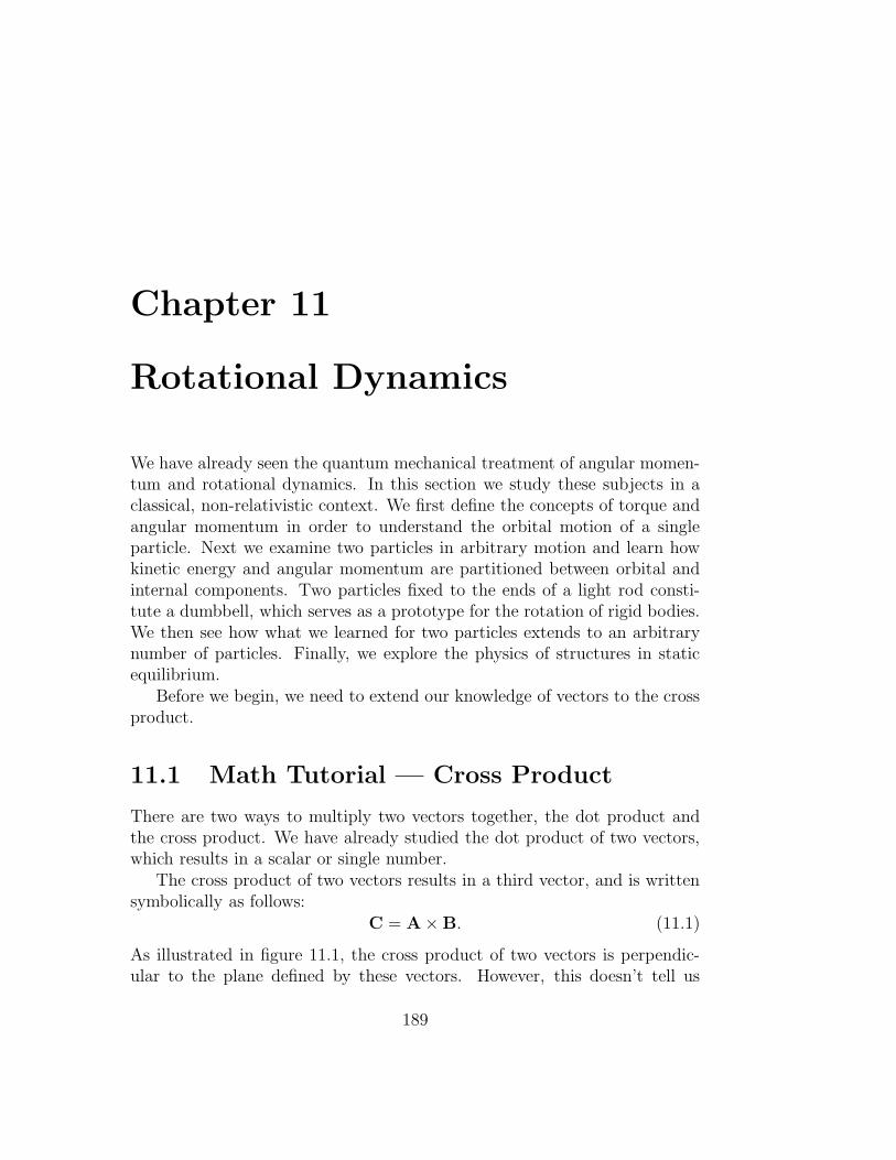
Chapter 11
Rotational Dynamics
We have already seen the quantum mechanical treatment of angular momen-tum and rotational dynamics. In this section we study these subjects in aclassical, non-relativistic context. We first define the concepts of torque andangular momentum in order to understand the orbital motion of a singleparticle. Next we examine two particles in arbitrary motion and learn howkinetic energy and angular momentum are partitioned between orbital andinternal components. Two particles fixed to the ends of a light rod consti-tute a dumbbell, which serves as a prototype for the rotation of rigid bodies.We then see how what we learned for two particles extends to an arbitrarynumber of particles. Finally, we explore the physics of structures in staticequilibrium.
Before we begin, we need to extend our knowledge of vectors to the crossproduct.
11.1 Math Tutorial — Cross Product
There are two ways to multiply two vectors together, the dot product andthe cross product. We have already studied the dot product of two vectors,which results in a scalar or single number.
The cross product of two vectors results in a third vector, and is writtensymbolically as follows:
C = A× B. (11.1)
As illustrated in figure 11.1, the cross product of two vectors is perpendic-ular to the plane defined by these vectors. However, this doesn’t tell us
189

190 CHAPTER 11. ROTATIONAL DYNAMICS
A
C
B
θ
Figure 11.1: Illustration of the cross product of two vectors A and B. Theresulting vector C is perpendicular to the plane defined by A and B.
whether the resulting vector in figure 11.1 points upward out of the plane ordownward. This ambiguity is resolved using the right-hand rule:
1. Point the uncurled fingers of your right hand along the direction of thefirst vector A.
2. Rotate your arm until you can curl your fingers in the direction of thesecond vector B.
3. Your stretched out thumb now points in the direction of the cross prod-uct vector C.
The magnitude of the cross product is given by
|C| = |A||B| sin(θ), (11.2)
where |A| and |B| are the magnitudes of A and B, and θ is the angle betweenthese two vectors. Note that the magnitude of the cross product is zerowhen the vectors are parallel or anti-parallel, and maximum when they areperpendicular. This contrasts with the dot product, which is maximum forparallel vectors and zero for perpendicular vectors.
Notice that the cross product does not commute, i. e., the order of thevectors is important. In particular, it is easy to show using the right-handrule that
A× B = −B × A. (11.3)
An alternate way to compute the cross product is most useful when thetwo vectors are expressed in terms of components, i. e., A = (Ax, Ay.Az)

11.2. TORQUE AND ANGULAR MOMENTUM 191
M
r p
F
O
Figure 11.2: A mass M located at r relative to the origin O has momentum p
and has a force F applied to it. By the right-hand rule the torque τ = r×F
points out of the page, while the angular momentum L = r × p points intothe page.
and B = (Bx, By, Bz):
Cx = AyBz − AzBy
Cy = AzBx − AxBz
Cz = AxBy −AyBx. (11.4)
Notice that once you have the first of these equations, the other two can beobtained by cyclically permuting the indices, i. e., x→ y, y → z, and z → x.This is useful as a memory aid.
11.2 Torque and Angular Momentum
Torque is the action of a force F on a mass M which induces it to revolveabout some point, called the origin. It is defined
τ = r × F, (11.5)
where r is the position of the mass relative to the origin, as illustrated infigure 11.2.
Notice that the torque is zero in a number of circumstances. If the forcepoints directly toward or away from the origin, the cross product is zero,resulting in zero torque, even though the force is non-zero. Likewise, if

192 CHAPTER 11. ROTATIONAL DYNAMICS
r = 0, the torque is zero. Thus, a force acting at the origin produces notorque. Both of these limits make sense intuitively, since neither induces themass to revolve around the origin.
The angular momentum of a mass M relative to a point O is
L = r × p, (11.6)
where p is the ordinary kinetic momentum of the mass.1 The angular mo-mentum is zero if the motion of the object is directly towards or away fromthe origin, or if it is located at the origin.
If we take the cross product of the position vector and Newton’s secondlaw, we obtain an equation that relates torque and angular momentum:
r × F = r ×dp
dt=
d
dt(r× p) −
dr
dt× p. (11.7)
The second term on the right side of the above equation is zero because dr/dtequals the velocity of the mass, which is parallel to its momentum and thecross product of two parallel vectors is zero. This equation can therefore bewritten
τ =dL
dt(Newton’s second law for rotation). (11.8)
It is the rotational version of Newton’s second law.For both torque and angular momentum the location of the origin is
arbitrary, and is generally chosen for maximum convenience. However, itis necessary to choose the same origin for both the torque and the angularmomentum.
For the case of a central force, i. e., one which acts along the line ofcenters between two objects (such as gravity), there often exists a particularlyconvenient choice of origin. Imagine a planet revolving around the sun, asillustrated in figure 11.3. If the origin is placed at the center of the sun (whichis assumed not to move under the influence of the planet’s gravity), then thetorque exerted on the planet by the sun’s gravity is zero, which means thatthe angular momentum of the planet about the center of the sun is constantin time. No other choice of origin would yield this convenient result.
1In the presence of a potential momentum we would have to distinguish between totaland kinetic momentum. This in turn would lead to a distinction between total and kineticangular momentum. We will assume that no potential momentum exists here, so that thisdistinction need not be made.

11.2. TORQUE AND ANGULAR MOMENTUM 193
O F
p
Figure 11.3: A convenient choice of origin for a planet (right-hand sphere)revolving around the sun is simply the center of the sun. In this case thetorque of the sun’s gravitational force on the planet is zero.
F12
F21M1
M2O
Figure 11.4: Scenario for the non-conservation of angular momentum.
We already know about two fundamental conservation laws — those ofenergy and linear momentum. We believe that angular momentum is simi-larly conserved in isolated systems. In other words, particles can exchangeangular momentum between themselves, but the vector sum of the angularmomentum of all the particles in a system isolated from outside influencesmust remain constant.
Conservation of angular momentum is not an automatic consequence ofthe conservation of linear momentum, even though the governing equation(11.8) for angular momentum is derived from Newton’s second law. As anexample, figure 11.4 shows a hypothetical situation in which the force of M1
on M2 is equal in magnitude but opposite in sign to the force of M2 on M1, i.

194 CHAPTER 11. ROTATIONAL DYNAMICS
r ’1
r ’2d1
d2
M1
M2
center of massO
r
r
Rcm
1
2
Figure 11.5: Two particles of mass M1 and M2 with M2 > M1.
e., Newton’s third law holds, and the sum of the momenta of the two massesis conserved. However, because the forces are non-central, the masses revolvemore and more rapidly with time about the origin, and angular momentum isnot conserved. This scenario is impossible if angular momentum is conserved.
11.3 Two Particles
Suppose we wish to apply Newton’s second law to two particles consideredtogether as a single system. As we showed previously, only external forcesact on the total momentum, ptotal = p1 + p2, of the two particles:
Fexternal =dptotal
dt. (11.9)
Let’s write the total non-relativistic momentum of the two particles in aspecial way:
ptotal = M1v1 +M2v2 = Mtotal
(
M1v1 +M2v2
Mtotal
)
≡ MtotalVcm, (11.10)
where Mtotal = M1 + M2. The quantity Vcm is the velocity of the center of
mass and can be expressed as the time derivative of the position of the center
of mass, Rcm,
Vcm =dRcm
dt, (11.11)
where
Rcm =M1r1 +M2r2
Mtotal. (11.12)

11.3. TWO PARTICLES 195
We now see how the kinetic energy and the angular momentum of thetwo particles may be split into two parts, one having to do with the motionof the center of mass of the two particles, the other having to do with themotion of the two particles relative their center of mass. Figure 11.5 showsgraphically how the vectors r′1 = r1 − Rcm and r′2 = r2 − Rcm are defined.These vectors represent the positions of the two particles relative to the centerof mass. Substitution into equation (11.12) shows that M1r
′
1 + M2r′
2 = 0.This leads to the conclusion that M1d1 = M2d2 in figure 11.5. We also definethe velocity of each mass relative to the center of mass as v′
1= dr′
1/dt and
v′
2 = dr′2/dt, and we therefore have M1v′
1 +M2v′
2 = 0.
The total kinetic energy is just the sum of the kinetic energies of the twoparticles, K = M1v
21/2 +M2v
22/2, where v1 and v2 are the magnitudes of the
corresponding velocity vectors. Substitution of v1 = Vcm + v′
1etc., into the
kinetic energy formula and rearranging yields
Ktotal = Ktrans +Kintern = [MtotalV2
cm/2] + [M1v′2
1/2 +M2v
′2
2/2]. (11.13)
Terms like Vcm · v′
1 cancel out because M1v′
1 +M2v′
2 = 0.
The first term on the right side of equation (11.13) in square bracketsis the kinetic energy the two particles would have if all of the mass wereconcentrated at the center of mass. The second term is the kinetic energy itwould have if it were observed from a reference frame in which the center ofmass is stationary. The first is called the translational kinetic energy of thesystem while the second is called the internal kinetic energy.
The angular momentum of the two particles is just the sum of the angularmomenta of the two masses: Ltotal = M1r1 × v1 +M2r2 × v2. By reasoningsimilar to the case of kinetic energy, we can rewrite this as
Ltotal = Lorb +Lspin = [MtotalRcm×Vcm]+ [M1r′
1×v′
1+M2r
′
2×v′
2]. (11.14)
The first term in square brackets on the right is called the orbital angular
momentum while the second term is called the spin angular momentum. Theformer is the angular momentum the system would have if all the mass wereconcentrated at the center of mass, while the latter is the angular momentumof motion about the center of mass.
Interestingly, the idea of center of mass and the corresponding split ofkinetic energy and angular momentum into orbital and spin parts has nouseful relativistic generalization. This is due to the factor of γ ≡ (1 −

196 CHAPTER 11. ROTATIONAL DYNAMICS
v1
v2
d1
M1
M2
d2
ω
Figure 11.6: Definition sketch for the rotating dumbbell attached to an axlelabeled ω. The axle attaches to the crossbar at the center of mass.
v2/c2)−1/2 in the relativistic definition of momentum, which means that
dmx
dt6= p (relativistic case). (11.15)
11.4 The Uneven Dumbbell
So far we have put no restrictions on the movements of the two particles.An interesting special case occurs when the particles are connected by alightweight, rigid rod, giving us a dumbbell. In order to further simplifythings, we assume that the rod is connected rigidly to a fixed axle at thecenter of mass of the two particles, as shown in figure 11.6. The massesconstituting the ends of the dumbbell are therefore free to revolve in circlesabout the axle, but they are prevented from executing any other motion.The key effect of this constraint is that both masses rotate about the axlewith the same angular frequency ω.
If the particles are respectively distances d1 and d2 from the axle, thentheir speeds are v1 = d1ω and v2 = d2ω. Thus the kinetic energy of therotating dumbbell is
Kintern =1
2M1v
2
1+
1
2M2v
2
2=
1
2Iω2 (fixed axle), (11.16)
where I = M1d21
+ M2d22
is called the moment of inertia. Similarly, themagnitude of the spin angular momentum, which is a vector parallel to the

11.5. MANY PARTICLES 197
axle, is
Lspin = M1d1v1 +M2d2v2 = Iω (fixed axle). (11.17)
Finally, Newton’s second law for rotation becomes
τ =dLspin
dt=dIω
dt= I
dω
dt(fixed axle), (11.18)
where τ is the component of torque along the rotation axis.
Note that the rightmost expression in equation (11.18) assumes that I isconstant, which only is true if d1 and d2 are constant – i. e., the dumbbellmust truly be rigid.
11.5 Many Particles
The generalization from two particles to many particles is quite easy in prin-ciple. If a subscripted i indicates the value of a quantity for the ith particle,then the center of mass is given by
Rcm =1
Mtotal
∑
i
Miri (11.19)
where
Mtotal =∑
i
Mi. (11.20)
Furthermore, if we define r′i = ri − Rcm, etc., then the kinetic energy is just
Ktotal = MtotalV2
cm/2 +∑
i
Miv′2
i /2 (11.21)
and the angular momentum is
Ltotal = MtotalRcm × Vcm +∑
i
Mir′
i × v′
i. (11.22)
In other words, both the kinetic energy and the angular momentum can beseparated into a part due to the overall motion of the system plus a part dueto motions of system components relative to the center of mass, just as forthe case of the dumbbell.

198 CHAPTER 11. ROTATIONAL DYNAMICS
11.6 Rigid Bodies
For a rigid body rotating about a fixed axle, the moment of inertia is
I =∑
i
Mid2
i , (11.23)
where di is the perpendicular distance of the ith particle from the axle. Equa-tions (11.16)-(11.18) are valid for a rigid body consisting of many particles.Furthermore, the moment of inertia is constant in this case, so it can betaken out of the time derivative:
τ =dIω
dt= I
dω
dt= Iα (fixed axle, constant I). (11.24)
The quantity α = dω/dt is called the angular acceleration.The sum in the equation for the moment of inertia can be converted to
an integral for a continuous distribution of mass. We shall not pursue thishere, but simply quote the results for a number of solid objects of uniformdensity:
• For rotation of a sphere of mass M and radius R about an axis piercingits center: I = 2MR2/5.
• For rotation of a cylinder of mass M and radius R about its axis ofsymmetry: I = MR2/2.
• For rotation of a thin rod of mass M and length L about an axisperpendicular to the rod passing through its center: I = ML2/12.
• For rotation of an annulus of mass M , inner radius Ra, and outer radiusRb about its axis of symmetry: I = M(R2
a +R2b)/2.
11.7 Statics
If a rigid body is initially at rest, it will remain at rest if and only if thesum of all the forces and the sum of all the torques acting on the body arezero. As an example, a mass balance with arms of differing length is shownin figure 11.7. The balance beam is subject to three forces pointing upwardor downward, the tension T in the string from which the beam is suspendedand the weights M1g and M2g exerted on the beam by the two suspended

11.7. STATICS 199
M1g M2g
MM1 2
d1 d2
T
asymmetric balancebeampivot point for
torque calculation
Figure 11.7: Asymmetric mass balance. We assume that the balance beamis massless.
masses. The parameter g is the local gravitational field and the balancebeam itself is assumed to have negligible mass. Taking upward as positive,the force condition for static equilibrium is
T −M1g −M2g = 0 (zero net force). (11.25)
Defining a counterclockwise torque to be positive, the torque balance com-puted about the pivot point in figure 11.7 is
τ = M1gd1 −M2gd2 = 0 (zero torque), (11.26)
where d1 and d2 are the lengths of the beam arms.The first of the above equations shows that the tension in the string must
beT = (M1 +M2)g, (11.27)
while the second shows thatM1
M2
=d2
d1
. (11.28)
Thus, the tension in the string is just equal to the weight of the massesattached to the balance beam, while the ratio of the two masses equals theinverse ratio of the associated beam arm lengths.

200 CHAPTER 11. ROTATIONAL DYNAMICS
RR’ vv’
Figure 11.8: Trajectory of a mass on a frictionless table attached to a stringwhich passes through a hole in the table. The string is drawing the mass in.
11.8 Problems
1. Show using the component form of the cross product given by equation(11.4) that A ×B = −B × A.
2. A mass M is sliding on a frictionless table, but is attached to a stringwhich passes through a hole in the center of the table as shown in figure11.8. The string is gradually drawn in so the mass traces out a spiralpattern as shown in figure 11.8. The initial distance of the mass fromthe hole in the table is R and its initial tangential velocity is v. Afterthe string is drawn in, the mass is a distance R′ from the hole and itstangential velocity is v′.
(a) Given R, v, and R′, find v′.
(b) Compute the change in the kinetic energy of the mass in goingfrom radius R to radius R′.
(c) If the above change is non-zero, determine where the extra energycame from.
3. A car of mass 1000 kg is heading north on a road at 30 m s−1 whichpasses 2 km east of the center of town.
(a) Compute the angular momentum of the car about the center oftown when the car is directly east of the town.
(b) Compute the angular momentum of the car about the center oftown when it is 3 km north of the above point.
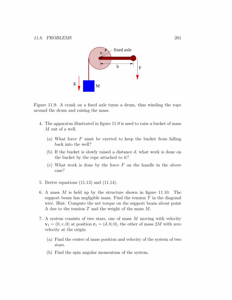
11.8. PROBLEMS 201
F
gM
a
b
fixed axle
Figure 11.9: A crank on a fixed axle turns a drum, thus winding the ropearound the drum and raising the mass.
4. The apparatus illustrated in figure 11.9 is used to raise a bucket of massM out of a well.
(a) What force F must be exerted to keep the bucket from fallingback into the well?
(b) If the bucket is slowly raised a distance d, what work is done onthe bucket by the rope attached to it?
(c) What work is done by the force F on the handle in the abovecase?
5. Derive equations (11.13) and (11.14).
6. A mass M is held up by the structure shown in figure 11.10. Thesupport beam has negligible mass. Find the tension T in the diagonalwire. Hint: Compute the net torque on the support beam about pointA due to the tension T and the weight of the mass M .
7. A system consists of two stars, one of mass M moving with velocityv1 = (0, v, 0) at position r1 = (d, 0, 0), the other of mass 2M with zerovelocity at the origin.
(a) Find the center of mass position and velocity of the system of twostars.
(b) Find the spin angular momentum of the system.

202 CHAPTER 11. ROTATIONAL DYNAMICS
M
θ
dg
support beam
TA
Figure 11.10: A mass is supported by the tension in the diagonal wire. Thesupport beam is free to pivot at point A.
M
T T21
2d d
d
Figure 11.11: A mass is supported by two strings.

11.8. PROBLEMS 203
F
B
A
M
LD
θ
Figure 11.12: A ladder leaning against a wall is held in place by friction withthe floor.
(c) Find the internal kinetic energy of the system.
8. A solid disk is rolling down a ramp tilted an angle θ from the horizontal.Compute the acceleration of the disk down the ramp and compare itwith the acceleration of a block sliding down the ramp without friction.
9. A mass M is suspended from the ceiling by two strings as shown infigure 11.11. Find the tensions in the strings.
10. A man of mass M is a distance D up a ladder of length L which makesan angle θ with respect to the vertical wall as shown in figure 11.12.Take the mass of the ladder to be negligible. Find the force F neededto keep the ladder from sliding if the wall and floor are frictionless andtherefore can only exert normal forces A and B on the ladder.

204 CHAPTER 11. ROTATIONAL DYNAMICS
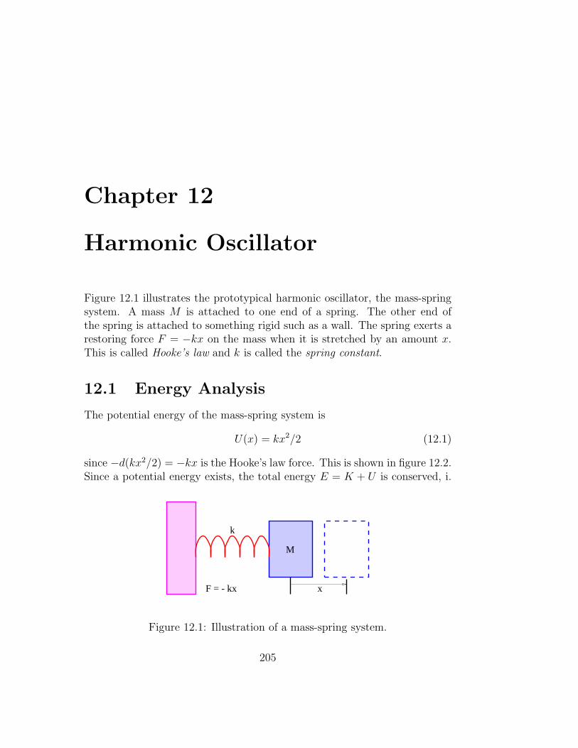
Chapter 12
Harmonic Oscillator
Figure 12.1 illustrates the prototypical harmonic oscillator, the mass-springsystem. A mass M is attached to one end of a spring. The other end ofthe spring is attached to something rigid such as a wall. The spring exerts arestoring force F = −kx on the mass when it is stretched by an amount x.This is called Hooke’s law and k is called the spring constant.
12.1 Energy Analysis
The potential energy of the mass-spring system is
U(x) = kx2/2 (12.1)
since −d(kx2/2) = −kx is the Hooke’s law force. This is shown in figure 12.2.Since a potential energy exists, the total energy E = K + U is conserved, i.
k
M
xF = - kx
Figure 12.1: Illustration of a mass-spring system.
205

206 CHAPTER 12. HARMONIC OSCILLATOR
U(x)
E
U
K
x
turning points
Figure 12.2: Potential, kinetic, and total energy of a harmonic oscillatorplotted as a function of spring displacement x.
e., is constant in time. If the total energy is known, this provides a usefultool for determining how the kinetic energy varies with the position x of themass M : K(x) = E − U(x). Since the kinetic energy is expressed (non-relativistically) in terms of the velocity u as K = Mu2/2, the velocity at anypoint on the graph in figure 12.2 is
u = ±
(
2(E − U)
M
)1/2
. (12.2)
Given all this, it is fairly evident how the mass moves. From Hooke’slaw, the mass is always accelerating toward the equilibrium position, x = 0.However, at any point the velocity can be either to the left or the right. Atthe points where U(x) = E, the kinetic energy is zero. This occurs at theturning points
xTP = ±(
2E
k
)1/2
. (12.3)
If the mass is moving to the left, it slows down as it approaches the leftturning point. It stops when it reaches this point and begins to move to theright. It accelerates until it passes the equilibrium position and then begins todecelerate, stopping at the right turning point, accelerating toward the left,etc. The mass thus oscillates between the left and right turning points. (Notethat equations (12.2) and (12.3) are only true for the harmonic oscillator.)
How does the period of the oscillation depend on the total energy of thesystem? Notice that from equation (12.2) the maximum speed of the mass

12.2. ANALYSIS USING NEWTON’S LAWS 207
(i. e., the speed at x = 0) is equal to umax = (2E/M)1/2. The average speedmust be some fraction of this maximum value. Let us guess here that it ishalf the maximum speed:
uaverage ≈umax
2=(
E
2M
)1/2
(approximate). (12.4)
However, the distance d the mass has to travel for one full oscillation istwice the distance between turning points, or d = 4(2E/k)1/2. Therefore,the period of oscillation must be approximately
T ≈d
uaverage= 4
(
2E
k
)1/2 (2M
E
)1/2
= 8(
M
k
)1/2
(approximate). (12.5)
12.2 Analysis Using Newton’s Laws
The acceleration of the mass at any time is given by Newton’s second law:
a =d2x
dt2=
F
M= −
kx
M. (12.6)
An equation of this type is known as a differential equation since it involvesa derivative of the dependent variable x. Equations of this type are generallymore difficult to solve than algebraic equations, as there are no universaltechniques for solving all forms of such equations. In fact, it is fair to saythat the solutions of most differential equations were originally obtained byguessing!
We already have the basis on which to make an intelligent guess for thesolution to equation (12.6) since we know that the mass oscillates back andforth with a period that is independent of the amplitude of the oscillation. Afunction which might fill the bill is the sine function. Let us try substitutingx = sin(ωt), where ω is a constant, into this equation. The second derivativeof x with respect to t is −ω2 sin(ωt), so performing this substitution resultsin
−ω2 sin(ωt) = −k
Msin(ωt). (12.7)
Notice that the sine function cancels out, leaving us with −ω2 = −k/M . Theguess thus works if we set
ω =
(
k
M
)1/2
. (12.8)

208 CHAPTER 12. HARMONIC OSCILLATOR
d = d sin ω0 F t
k
M
xF = - k (x - d)
Figure 12.3: Illustration of a forced mass-spring oscillator. The left end ofthe spring is wiggled back and forth with an angular frequency ωF and amaximum amplitude d0.
The constant ω is the angular oscillation frequency for the oscillator,from which we infer the period of oscillation to be T = 2π(M/k)1/2. Thisagrees with the earlier approximate result of equation (12.5), except that theapproximation has a numerical factor of 8 rather than 2π ≈ 6. Thus, theearlier guess is only off by about 30%!
It is easy to show that x = A sin(ωt) is also a solution of equation (12.6),where A is any constant and ω = (k/M)1/2. This confirms that the oscillationfrequency and period are independent of amplitude. Furthermore, the cosinefunction is equally valid as a solution: x = B cos(ωt), where B is anotherconstant. In fact, the most general possible solution is just a combination ofthese two, i. e.,
x = A sin(ωt) +B cos(ωt). (12.9)
The values of A and B depend on the position and velocity of the mass attime t = 0.
12.3 Forced Oscillator
If we wiggle the left end of the spring by the amount d = d0 sin(ωF t), as infigure 12.3, rather than rigidly fixing it as in figure 12.1, we have a forced
harmonic oscillator. The constant d0 is the amplitude of the imposed wigglingmotion. The forcing frequency ωF is not necessarily equal to the natural orresonant frequency ω = (k/M)1/2 of the mass-spring system. Very differentbehavior occurs depending on whether ωF is less than, equal to, or greaterthan ω.
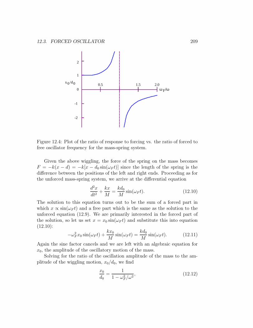
12.3. FORCED OSCILLATOR 209
ω F/ω
x0 /d 0
-1
-2
1.5 2.0
2
1
00.5
Figure 12.4: Plot of the ratio of response to forcing vs. the ratio of forced tofree oscillator frequency for the mass-spring system.
Given the above wiggling, the force of the spring on the mass becomesF = −k(x − d) = −k[x − d0 sin(ωF t)] since the length of the spring is thedifference between the positions of the left and right ends. Proceeding as forthe unforced mass-spring system, we arrive at the differential equation
d2x
dt2+kx
M=kd0
Msin(ωF t). (12.10)
The solution to this equation turns out to be the sum of a forced part inwhich x ∝ sin(ωF t) and a free part which is the same as the solution to theunforced equation (12.9). We are primarily interested in the forced part ofthe solution, so let us set x = x0 sin(ωF t) and substitute this into equation(12.10):
−ω2
Fx0 sin(ωF t) +kx0
Msin(ωF t) =
kd0
Msin(ωF t). (12.11)
Again the sine factor cancels and we are left with an algebraic equation forx0, the amplitude of the oscillatory motion of the mass.
Solving for the ratio of the oscillation amplitude of the mass to the am-plitude of the wiggling motion, x0/d0, we find
x0
d0
=1
1 − ω2F/ω
2, (12.12)

210 CHAPTER 12. HARMONIC OSCILLATOR
where we have recognized that k/M = ω2, the square of the frequency of thefree oscillation. This function is plotted in figure 12.4.
Notice that if ωF < ω, the motion of the mass is in phase with the wig-gling motion and the amplitude of the mass oscillation is greater than theamplitude of the wiggling. As the forcing frequency approaches the natu-ral frequency of the oscillator, the response of the mass grows in amplitude.When the forcing is at the resonant frequency, the response is technicallyinfinite, though practical limits on the amplitude of the oscillation will in-tervene in this case — for instance, the spring cannot stretch or shrink aninfinite amount. In many cases friction will act to limit the response of themass to forcing near the resonant frequency. When the forcing frequency isgreater than the natural frequency, the mass actually moves in the oppositedirection of the wiggling motion — i. e., the response is out of phase withthe forcing. The amplitude of the response decreases as the forcing frequencyincreases above the resonant frequency.
Forced and free harmonic oscillators form an important part of manyphysical systems. For instance, any elastic material body such as a bridgeor an airplane wing has harmonic oscillatory modes. A common engineeringproblem is to ensure that such modes are damped by friction or some otherphysical mechanism when there is a possibility of exitation of these modesby naturally occurring processes. A number of disasters can be traced to afailure to properly account for oscillatory forcing in engineered structures.
12.4 Quantum Mechanical Harmonic Oscilla-
tor
The quantum mechanical harmonic oscillator shares the characteristic ofother quantum mechanical bound state problems in that the total energycan take on only discrete values. Calculation of these values is too diffi-cult for this course, but the problem is sufficiently important to warrantreporting the results here. The energies accessible to a quantum mechanicalmass-spring system are given by the formula
En = (n+ 1/2)h(k/M)1/2, n = 0, 1, 2, . . . . (12.13)
In other words, the energy difference between successive quantum mechan-ical energy levels in this case is constant and equals the classical resonantfrequency for the oscillator, ω = (k/M)1/2.

12.5. PROBLEMS 211
L
M
θ
x
Figure 12.5: The pendulum as a harmonic oscillator.
12.5 Problems
1. Consider the pendulum in figure 12.5. The mass M moves along an arcwith x denoting the distance along the arc from the equilibrium point.
(a) Find the component of the gravitational force tangent to the arc(and thus in the direction of motion of the mass) as a functionof the angle θ. Use the small angle approximation on sin(θ) tosimplify this answer.
(b) Get the force in terms of x rather than θ. (Recall that θ = x/L.)
(c) Use Newton’s second law for motion in the x direction (i. e., alongthe arc followed by the mass) to get the equation of motion forthe mass.
(d) Solve the equation of motion using the solution to the mass-springproblem as a guide.
2. An oscillator (non-harmonic) has the potential energy function U(x) =Cx4, where C is a constant. How does the oscillation frequency dependon energy? Explain your reasoning.
3. A massless particle is confined to a box of length a. (Think of a photonbetween two mirrors.) Treating the particle classically, compute the

212 CHAPTER 12. HARMONIC OSCILLATOR
period of one round trip from one end of the box to the other and backagain. From this compute an angular frequency for the oscillation ofthis particle in the box. Does this frequency depend on the particle’senergy?
4. Compute the ground state energy Eground of a massless particle in abox of length a using quantum mechanics. Compare Eground/h withthe angular frequency computed in the previous problem.

Appendix A
Constants
This appendix lists various useful constants.
A.1 Constants of Nature
Symbol Value Meaning
h 6.63 × 10⁻³⁴ J s Planck’s constanth 1.06 × 10⁻³⁴ J s h/(2π)c 3 × 10⁸ m s−1 speed of lightG 6.67 × 10⁻¹¹ m3 s−2 kg−1 universal gravitational constantkB 1.38 × 10⁻²³ J K−1 Boltzmann’s constantσ 5.67 × 10⁻⁸ W m−2 K−4 Stefan-Boltzmann constantK 3.67 × 10¹¹ s−1 K−1 thermal frequency constantǫ0 8.85 × 10⁻¹² C2 N−1 m−2 permittivity of free spaceµ0 4π × 10−7 N s2 C−2 permeability of free space (= 1/(ǫ0c
2)).
A.2 Properties of Stable Particles
Symbol Value Meaning
e 1.60 × 10⁻¹⁹ C fundamental unit of chargeme 9.11 × 10⁻³¹ kg = 0.511 MeV mass of electronmp 1.672648× 10⁻²⁷ kg = 938.280 MeV mass of protonmn 1.674954× 10⁻²⁷ kg = 939.573 MeV mass of neutron
213

214 APPENDIX A. CONSTANTS
A.3 Properties of Solar System Objects
Symbol Value Meaning
Me 5.98 × 1024 kg mass of earthMm 7.36 × 10²² kg mass of moonMs 1.99 × 1030 kg mass of sunRe 6.37 × 10⁶ m radius of earthRm 1.74 × 10⁶ m radius of moonRs 6.96 × 10⁸ m radius of sunDm 3.82 × 10⁸ m earth-moon distanceDs 1.50 × 10¹¹ m earth-sun distanceg 9.81 m s−2 earth’s surface gravity
A.4 Miscellaneous Conversions
1 lb = 4.448 N1 ft = 0.3048 m1 mph = 0.4470 m s−1
1 eV = 1.60 × 10⁻¹⁹ J

Appendix B
GNU Free Documentation
License
Version 1.1, March 2000
Copyright c© 2000 Free Software Foundation, Inc.59 Temple Place, Suite 330, Boston, MA 02111-1307 USAEveryone is permitted to copy and distribute verbatim copies of this licensedocument, but changing it is not allowed.
Preamble
The purpose of this License is to make a manual, textbook, or other writtendocument “free” in the sense of freedom: to assure everyone the effectivefreedom to copy and redistribute it, with or without modifying it, eithercommercially or noncommercially. Secondarily, this License preserves for theauthor and publisher a way to get credit for their work, while not beingconsidered responsible for modifications made by others.
This License is a kind of “copyleft”, which means that derivative worksof the document must themselves be free in the same sense. It complementsthe GNU General Public License, which is a copyleft license designed for freesoftware.
We have designed this License in order to use it for manuals for freesoftware, because free software needs free documentation: a free programshould come with manuals providing the same freedoms that the software
215
216 APPENDIX B. GNU FREE DOCUMENTATION LICENSE
does. But this License is not limited to software manuals; it can be usedfor any textual work, regardless of subject matter or whether it is publishedas a printed book. We recommend this License principally for works whosepurpose is instruction or reference.
B.1 Applicability and Definitions
This License applies to any manual or other work that contains a noticeplaced by the copyright holder saying it can be distributed under the termsof this License. The “Document”, below, refers to any such manual or work.Any member of the public is a licensee, and is addressed as “you”.
A “Modified Version” of the Document means any work containing theDocument or a portion of it, either copied verbatim, or with modificationsand/or translated into another language.
A “Secondary Section” is a named appendix or a front-matter section ofthe Document that deals exclusively with the relationship of the publishersor authors of the Document to the Document’s overall subject (or to relatedmatters) and contains nothing that could fall directly within that overallsubject. (For example, if the Document is in part a textbook of mathematics,a Secondary Section may not explain any mathematics.) The relationshipcould be a matter of historical connection with the subject or with relatedmatters, or of legal, commercial, philosophical, ethical or political positionregarding them.
The “Invariant Sections” are certain Secondary Sections whose titles aredesignated, as being those of Invariant Sections, in the notice that says thatthe Document is released under this License.
The “Cover Texts” are certain short passages of text that are listed, asFront-Cover Texts or Back-Cover Texts, in the notice that says that theDocument is released under this License.
A “Transparent” copy of the Document means a machine-readable copy,represented in a format whose specification is available to the general pub-lic, whose contents can be viewed and edited directly and straightforwardlywith generic text editors or (for images composed of pixels) generic paintprograms or (for drawings) some widely available drawing editor, and that issuitable for input to text formatters or for automatic translation to a varietyof formats suitable for input to text formatters. A copy made in an other-wise Transparent file format whose markup has been designed to thwart or

B.2. VERBATIM COPYING 217
discourage subsequent modification by readers is not Transparent. A copythat is not “Transparent” is called “Opaque”.
Examples of suitable formats for Transparent copies include plain ASCIIwithout markup, Texinfo input format, LATEX input format, SGML or XMLusing a publicly available DTD, and standard-conforming simple HTML de-signed for human modification. Opaque formats include PostScript, PDF,proprietary formats that can be read and edited only by proprietary wordprocessors, SGML or XML for which the DTD and/or processing tools arenot generally available, and the machine-generated HTML produced by someword processors for output purposes only.
The “Title Page” means, for a printed book, the title page itself, plussuch following pages as are needed to hold, legibly, the material this Licenserequires to appear in the title page. For works in formats which do not haveany title page as such, “Title Page” means the text near the most prominentappearance of the work’s title, preceding the beginning of the body of thetext.
B.2 Verbatim Copying
You may copy and distribute the Document in any medium, either commer-cially or noncommercially, provided that this License, the copyright notices,and the license notice saying this License applies to the Document are re-produced in all copies, and that you add no other conditions whatsoever tothose of this License. You may not use technical measures to obstruct orcontrol the reading or further copying of the copies you make or distribute.However, you may accept compensation in exchange for copies. If you dis-tribute a large enough number of copies you must also follow the conditionsin section 3.
You may also lend copies, under the same conditions stated above, andyou may publicly display copies.
B.3 Copying in Quantity
If you publish printed copies of the Document numbering more than 100,and the Document’s license notice requires Cover Texts, you must enclosethe copies in covers that carry, clearly and legibly, all these Cover Texts:

218 APPENDIX B. GNU FREE DOCUMENTATION LICENSE
Front-Cover Texts on the front cover, and Back-Cover Texts on the backcover. Both covers must also clearly and legibly identify you as the publisherof these copies. The front cover must present the full title with all words ofthe title equally prominent and visible. You may add other material on thecovers in addition. Copying with changes limited to the covers, as long asthey preserve the title of the Document and satisfy these conditions, can betreated as verbatim copying in other respects.
If the required texts for either cover are too voluminous to fit legibly,you should put the first ones listed (as many as fit reasonably) on the actualcover, and continue the rest onto adjacent pages.
If you publish or distribute Opaque copies of the Document number-ing more than 100, you must either include a machine-readable Transparentcopy along with each Opaque copy, or state in or with each Opaque copy apublicly-accessible computer-network location containing a complete Trans-parent copy of the Document, free of added material, which the generalnetwork-using public has access to download anonymously at no charge us-ing public-standard network protocols. If you use the latter option, you musttake reasonably prudent steps, when you begin distribution of Opaque copiesin quantity, to ensure that this Transparent copy will remain thus accessibleat the stated location until at least one year after the last time you distributean Opaque copy (directly or through your agents or retailers) of that editionto the public.
It is requested, but not required, that you contact the authors of theDocument well before redistributing any large number of copies, to give thema chance to provide you with an updated version of the Document.
B.4 Modifications
You may copy and distribute a Modified Version of the Document under theconditions of sections 2 and 3 above, provided that you release the ModifiedVersion under precisely this License, with the Modified Version filling therole of the Document, thus licensing distribution and modification of theModified Version to whoever possesses a copy of it. In addition, you mustdo these things in the Modified Version:
• Use in the Title Page (and on the covers, if any) a title distinct from thatof the Document, and from those of previous versions (which should, if

B.4. MODIFICATIONS 219
there were any, be listed in the History section of the Document). Youmay use the same title as a previous version if the original publisher ofthat version gives permission.
• List on the Title Page, as authors, one or more persons or entitiesresponsible for authorship of the modifications in the Modified Version,together with at least five of the principal authors of the Document (allof its principal authors, if it has less than five).
• State on the Title page the name of the publisher of the ModifiedVersion, as the publisher.
• Preserve all the copyright notices of the Document.
• Add an appropriate copyright notice for your modifications adjacent tothe other copyright notices.
• Include, immediately after the copyright notices, a license notice givingthe public permission to use the Modified Version under the terms ofthis License, in the form shown in the Addendum below.
• Preserve in that license notice the full lists of Invariant Sections andrequired Cover Texts given in the Document’s license notice.
• Include an unaltered copy of this License.
• Preserve the section entitled “History”, and its title, and add to it anitem stating at least the title, year, new authors, and publisher of theModified Version as given on the Title Page. If there is no sectionentitled “History” in the Document, create one stating the title, year,authors, and publisher of the Document as given on its Title Page, thenadd an item describing the Modified Version as stated in the previoussentence.
• Preserve the network location, if any, given in the Document for publicaccess to a Transparent copy of the Document, and likewise the networklocations given in the Document for previous versions it was based on.These may be placed in the “History” section. You may omit a networklocation for a work that was published at least four years before theDocument itself, or if the original publisher of the version it refers togives permission.

220 APPENDIX B. GNU FREE DOCUMENTATION LICENSE
• In any section entitled “Acknowledgements” or “Dedications”, preservethe section’s title, and preserve in the section all the substance and toneof each of the contributor acknowledgements and/or dedications giventherein.
• Preserve all the Invariant Sections of the Document, unaltered in theirtext and in their titles. Section numbers or the equivalent are notconsidered part of the section titles.
• Delete any section entitled “Endorsements”. Such a section may notbe included in the Modified Version.
• Do not retitle any existing section as “Endorsements” or to conflict intitle with any Invariant Section.
If the Modified Version includes new front-matter sections or appendicesthat qualify as Secondary Sections and contain no material copied from theDocument, you may at your option designate some or all of these sectionsas invariant. To do this, add their titles to the list of Invariant Sections inthe Modified Version’s license notice. These titles must be distinct from anyother section titles.
You may add a section entitled “Endorsements”, provided it containsnothing but endorsements of your Modified Version by various parties – forexample, statements of peer review or that the text has been approved byan organization as the authoritative definition of a standard.
You may add a passage of up to five words as a Front-Cover Text, and apassage of up to 25 words as a Back-Cover Text, to the end of the list of CoverTexts in the Modified Version. Only one passage of Front-Cover Text andone of Back-Cover Text may be added by (or through arrangements madeby) any one entity. If the Document already includes a cover text for thesame cover, previously added by you or by arrangement made by the sameentity you are acting on behalf of, you may not add another; but you mayreplace the old one, on explicit permission from the previous publisher thatadded the old one.
The author(s) and publisher(s) of the Document do not by this Licensegive permission to use their names for publicity for or to assert or implyendorsement of any Modified Version.

B.5. COMBINING DOCUMENTS 221
B.5 Combining Documents
You may combine the Document with other documents released under thisLicense, under the terms defined in section 4 above for modified versions,provided that you include in the combination all of the Invariant Sectionsof all of the original documents, unmodified, and list them all as InvariantSections of your combined work in its license notice.
The combined work need only contain one copy of this License, and mul-tiple identical Invariant Sections may be replaced with a single copy. If thereare multiple Invariant Sections with the same name but different contents,make the title of each such section unique by adding at the end of it, inparentheses, the name of the original author or publisher of that section ifknown, or else a unique number. Make the same adjustment to the sectiontitles in the list of Invariant Sections in the license notice of the combinedwork.
In the combination, you must combine any sections entitled “History”in the various original documents, forming one section entitled “History”;likewise combine any sections entitled “Acknowledgements”, and any sec-tions entitled “Dedications”. You must delete all sections entitled “Endorse-ments.”
B.6 Collections of Documents
You may make a collection consisting of the Document and other documentsreleased under this License, and replace the individual copies of this Licensein the various documents with a single copy that is included in the collection,provided that you follow the rules of this License for verbatim copying of eachof the documents in all other respects.
You may extract a single document from such a collection, and distributeit individually under this License, provided you insert a copy of this Licenseinto the extracted document, and follow this License in all other respectsregarding verbatim copying of that document.
B.7 Aggregation With Independent Works
A compilation of the Document or its derivatives with other separate and in-dependent documents or works, in or on a volume of a storage or distribution
222 APPENDIX B. GNU FREE DOCUMENTATION LICENSE
medium, does not as a whole count as a Modified Version of the Document,provided no compilation copyright is claimed for the compilation. Such acompilation is called an “aggregate”, and this License does not apply to theother self-contained works thus compiled with the Document, on account oftheir being thus compiled, if they are not themselves derivative works of theDocument.
If the Cover Text requirement of section 3 is applicable to these copies ofthe Document, then if the Document is less than one quarter of the entireaggregate, the Document’s Cover Texts may be placed on covers that sur-round only the Document within the aggregate. Otherwise they must appearon covers around the whole aggregate.
B.8 Translation
Translation is considered a kind of modification, so you may distribute trans-lations of the Document under the terms of section 4. Replacing InvariantSections with translations requires special permission from their copyrightholders, but you may include translations of some or all Invariant Sectionsin addition to the original versions of these Invariant Sections. You may in-clude a translation of this License provided that you also include the originalEnglish version of this License. In case of a disagreement between the trans-lation and the original English version of this License, the original Englishversion will prevail.
B.9 Termination
You may not copy, modify, sublicense, or distribute the Document exceptas expressly provided for under this License. Any other attempt to copy,modify, sublicense or distribute the Document is void, and will automaticallyterminate your rights under this License. However, parties who have receivedcopies, or rights, from you under this License will not have their licensesterminated so long as such parties remain in full compliance.

B.10. FUTURE REVISIONS OF THIS LICENSE 223
B.10 Future Revisions of This License
The Free Software Foundation may publish new, revised versions of the GNUFree Documentation License from time to time. Such new versions will besimilar in spirit to the present version, but may differ in detail to addressnew problems or concerns. See http://www.gnu.org/copyleft/.
Each version of the License is given a distinguishing version number. Ifthe Document specifies that a particular numbered version of this License ”orany later version” applies to it, you have the option of following the termsand conditions either of that specified version or of any later version thathas been published (not as a draft) by the Free Software Foundation. If theDocument does not specify a version number of this License, you may chooseany version ever published (not as a draft) by the Free Software Foundation.
ADDENDUM: How to use this License for your
documents
To use this License in a document you have written, include a copy of theLicense in the document and put the following copyright and license noticesjust after the title page:
Copyright c© YEAR YOUR NAME. Permission is granted tocopy, distribute and/or modify this document under the terms ofthe GNU Free Documentation License, Version 1.1 or any laterversion published by the Free Software Foundation; with the In-variant Sections being LIST THEIR TITLES, with the Front-Cover Texts being LIST, and with the Back-Cover Texts beingLIST. A copy of the license is included in the section entitled“GNU Free Documentation License”.
If you have no Invariant Sections, write “with no Invariant Sections”instead of saying which ones are invariant. If you have no Front-Cover Texts,write “no Front-Cover Texts” instead of “Front-Cover Texts being LIST”;likewise for Back-Cover Texts.
If your document contains nontrivial examples of program code, we rec-ommend releasing these examples in parallel under your choice of free soft-ware license, such as the GNU General Public License, to permit their usein free software.

224 APPENDIX B. GNU FREE DOCUMENTATION LICENSE

Appendix C
History
• Prehistory: The text was developed to this stage over a period of about5 years as course notes to Physics 131/132 at New Mexico Tech byDavid J. Raymond, with input from Alan M. Blyth. The course wastaught by Raymond and Blyth and by David J. Westpfahl at NewMexico Tech.
• 14 May 2001: First “copylefted” version of this text.
• 14 May 2003: Numerous small changes and corrections were made.
• 25 June 2004: More small corrections to volume one.
• 14 December 2004: More small corrections to volume one.
• 9 May 2005: More small corrections to volume two.
• 7 April 2006: More small corrections to both volumes.
• 7 July 2006: Finish volume 2 corrections for the coming year.
• 2 July 2008: Finish volume 1 corrections for fall 2008.
•
225