A Quantization Approach to the CreditExposure Estimation

Michele Bonollo, Credito Trevigiano and IMT Lucca - michele.bonollo@imtlucca.itLuca Di Persio, Dept. Informatics - University of Verona - luca.dipersio@univr.it

Immacolata Oliva, Dept. Informatics - University of Verona - Immacolata.Oliva@univr.itAndrea Semmoloni - a.semmoloni@gmail.com

AbstractThe present paper aims at giving a rigorous approach to Credit Counterparty Risk Estima-tion exploiting quantization techniques.

1 Introduction and Scope of the StudyThe financial crisis in 2007-2008, along with an increasing awareness about the differentsources of risk, allowed to focus at a deeper level the counterparty credit risk (CCR). CCRrefers to the situation when the counterparty A has a deal, mainly a derivative type suc asan option or a swap, subscribed with the counterparty B. We suppose that according to avaluation criteria based on market prices in the A perspective we observe positive Mark toMarket (MtM). It follows that A has a credit exposure with B, hence if B defaults and nofuture recovery rates and no collaterals were posted, then A loses exactly MtM, the cost forthe replacement of the defaulted position. Such type of risk is of particular interest withinthe so called Over The Counter (OTC) derivatives markets. We recall that OTC marketsare characterized by having all the transactions which are not listed in the stock exchange,but, instead, they are settled directly between the two counterpaties.

A slightly different perspective of CCR has to taken into account when in the risk man-agement field A evaluates ex-ante the risk belonging to the financial position underwrittenwith B. In such a case, since the possible default for B is a random event, both in time andalso concerning its magnitude, it turns out that the current MtM is a too rough measure ofthe credit exposure for A.

On the basis of the latter consideration, in what follows we will focus our attention onwhat is called Exposure At Deafult (EAD). EAD parameter can be seen as a sort of conser-vative expected value of the future MtM at the default time. An official way to estimate theEAD in various contest, has been given in the Basel framework, see [1], namely within theset of recommendations on banking laws and regulations issued by the Basel Committeeon Banking Supervision. Such an approach is based on the Expected Positive Exposure(EPE) evaluation, namely on a prudent probabilistic time average of the future MtM. EADfollows just as a multple, i.e. EAD = α · EPE.

Moreover, we recall that the international accounting standards require that in thederivatives evaluation a full fair value principle, see, e.g., [15], has to be satisfied.

1

If the the counterparty solvency level falls, we observe a downgrade in its rating and/oran increase in its spread, therefore the related OTC balance sheet evaluation has to embodythis effect. The latter implies that we have to adjust the MtM since it may decrease not onlydue to the usual market parameters, e.g. underlying price, underlying volatility, free riskrate, etc., but also for the credit spread volatility.

We refer to such an MtM adjustment, as Credit value Adjustment (CVA), and the re-lated adjusted fair value is sometimes called the full fair value. The adjusted MtM will bedenoted by MtMA and we have MtMA = MtM − CV A.

Even if the derivative has not been closed, the CVA effect can cause a loss in thebalance sheet, namely an unrealized loss. Some studies of the Basel Committe estimatethat 2/3 of the losses in the financial crisis years in the OTC sector were unrealized lossesin the evaluation process. The CVA loss is (or should be) absorbed by the balance sheet,while the CVA volatility must be faced by the regulatory capital. To this end, a new capitalcharge, the CVA charge, was introduced with the Basel III framework. For the accountingprinciples, see [14], while a detailed discussion about the capital charge can be found in[2].

The EAD and the CVA computations pose a lot of methodological, financial and nu-merical issues, as witnessed by huge amount of literature developed so far, see, e.g., [9],for a detailed review of these subjects.

The present paper aims not at discussing the usefulness of EAD/CVA measures, northe related underlyings or volatility models, moreover we will not concern with the analysisof data quality and data availability. Indeed we aim at studying the feasibility and the tradeoff accuracy vs. computational effort of the quantization approach for the EAD-estimation(EPE). Therefore our main goal is the numerical CCR analysis, while we addressed theCVA issue in a future work.

In particular we will consider a simple Black and Scholes model, without taking intoconsideration collateral parameters in order to focus the attention of the implemented nu-merical techniques.

The paper is organized as follows: Section 2 is a review of the EPE definition given bythe Basel Committee, in Section 3 we will give a description of the quantization approachto the EPE with some theoretical results, in Section 4 we describe some practical cases andwe give the set up of the associated numerical experiments, while in Section 5 we reportthe obtained numerical results along with their interpretation.

2 The Basel EPE definitionIn what follows we shall give a review about the Basel Committee guide lines concern-ing the estimation of the Exposure at Default, namely the EPE parameter. Let us set thefollowing notations that will be used throughout the paper

• taking into account a derivative maturity time 0 < T < +∞, we consider K ∈ N+

time steps 0 < t1 < t2 < · · · < tK which constitute the so called buckets array,denoted by BT,K , where usually, but not mandatory, tK = T .

• for every tk ∈ BT,K we denote by MtM (tk, Sk) := MtM (tk, Stk) the fair value(mark to market) of a derivative at time bucket tk, with respect to the underlyingvalue Sk at time tk. For the sake of simplicity, we denote by t0 = 0 the starting timeof our evaluation problem, hence considering the european case.

2

• for every tk ∈ BT,K we denote by MtM(tk, S

k)

:= MtM (tk, Stk) the the fair

value (mark to market) of a derivative at time bucket tk, with respect to the wholesample path Sk := St : 0 ≤ t ≤ tk, again considering an initial time t0 = 0.

• taking into account previous defintions, we indicate by ϕ = ϕ (T − tk, Sk,Θ) thepricing function for the given derivative, where Θ represents the set of parametersfrom which such a pricing function depends, e.g. the free risk rate r, the volatility σ,etc.

• we will use the notation φMtM to denote the mark to market value pricing function

Remark 1. We would like to underline that in the Black-Scholes framework the volatilitysurface has to be flat, which is not the case when considering real financial time series.It follows that the previously considered pricing function φ most likely depends from morethan the two mentioned parameters r and σ. In particular usually Θ ∈ Rn, with n > 2, theextra parameters being those characterizing the specific geometric structure of the volatilitysurface associated to the considered contingent claim.

As usual in the counterparty credit risk EAD estimation, we stress the role of the under-lying, while the other market parameters are assumed to be given, namely we assume thatthey are deterministic and known. As an example of the latter assumption we can considerthe case where both the unknown risk free rate and volatility values are substituted by theirdeterministic forward values.

In what follows we shall often use the notation k to indicate quantities of interestevaluated at the k − th time bucket tk, moreover

• we denote the Expected Exposure (EE) of the derivative by

EEk :=1

N

∑n=1..N

MtM (tk, Sk,n)+ ,

which is nothing but the arithmetic mean of N ∈ N+, Monte Carlo simulated MtMvalues, computed at the k − th time bucket tk, with respect to the underlyng S. Thepositive part operator (·)+is effective if we area managing a symmetric derivative,such as an interesest rate swap, or a portfolio of derivatives. For a single option, it isredundant, as the fair value of the option is always postive from the buy side situation,while the sell side does not imply couterparty risk and then it is out of context.

• we evaluate the expected positive exposure (EPE) by EPE :=∑K

k=1 EEk·∆k

T, where

∆k indicates the time space between two consecutive time buckets at k − th level.If the time buckets tk are equally spaced, then the formula reduces to EPE =1K

∑Kk=1EEk. Therefore the EPE value gives the time average of the EEk

• we setEEE1 := EE1 andEEEk = Max EEk, EEEk−1, for every k = 1, . . . , K.In particular EEEk is called the effective expected exposure and its non decreasingrule takes into account the fact that once the time decay effect reduces the MtM, andthe counterparty risk exposure accordingly, the bank applies a roll out with some newdeals

3

• we define the effected expected positive exposure (EEPE), by

EEPE :=

∑Kk=1EEEk ·∆k

T.

To avoid too many inessential regulatory details, we will work on the first quantities EEkand EPE, the others being just arithmetic modifications of them.

Remark 2. Let us point out that the definiton of EEk is taken from the Basel regulatoryframework.We find it quite strange, since instead of giving a theoretical principle and sug-gesting the Monte Carlo technique just as a possible computational tool, the simulationapproach is officially embedded in the general definition.

In what follows we shall rewrite previously defined quantities in continuous time, andwe add the index A to indicate the adjusted definitions. Moreover we consider the dynamicof the underlying St := Stt∈[0,T ], T ∈ R+ being some expiration date, to be the oneof an Itı¿œ processes defined on some filtered probability space

(Ω,F ,Ft∈[0,T ],P

). As an

example St being the solution of the stochastic differential equation defining the geometricBrownian motion, Ft∈[0,T ] is the natural filtration generated by a standard Brownian motionWt = Wt∈[0,T ] starting from a complete probability space (Ω,F ,P), where P could be theso called real world probability measure or, in a martingale approach to option pricing, see,e.g., [22, Ch.5], an equivalent risk neutral measure

• we set

EEAk := EP

[MtM (tk, Sk)

+] =

ˆϕ (tk, Sk,Θ) dP

∼=1

N

∑n=1..N

MtM (tk, Sk,n)+ = EEk = EEAk

(1)

• we define EPEA :=´EEA

t · dt =´ [´

ϕ (t, Sk,Θ) dP]· dt

In this new formulation the Basel definition is simply (one of the many) method to estimatethe expected fair value of the derivative in the future.

Remark 3. Which probability P to use in the calculation of EEk , i.e. a risk neutralprobability for the drift St vs. an historical real world probability, is beyond the scope ofour paper. For a detailed discussion, see, e.g., [8]

Remark 4. We can observe in the EPE definition that the discount factor, or numeraire, ismissing. It was not forgot, but this is one of the several conservative proxies used in therisk regulation.

If we adopt a simulation approach, for the underlying path construction we could, foreach simulation n, to generate a path with an array of points (xn,tk). This algorithm is calledpath-dependent simulation (PDS). Alternatively we could jointly, for each time bucket andeach simulation, generate our N · K points. This approach is referred as direct-jump tosimulation date (DJS). The figure below, taken from [20], well clarify the difference

Finally, we recall that in the risk managment application another quantity is very pop-ular in the practice, i.e. the PFEα (potential future esposure) a quantile based figure of theexreme risk. In a continuous setting

• PFE (α, tk) = MtM∗ : PMtM (tk, Sk)

+ ≥MtM∗

= 1− α

4

3 A short quantization reviewThe quantization technique is kown from several decades, and it comes from engineering,when facing the issue of converting an analogical signal, e.g. images, sounds, etc., in to adiscretized digital information. Other relevant fields are those of information compressionand statistical multidimensioanl clustering. For a classical reference of quantization werefer to see [11], while we refer to [16] for a survey of the related literature concerningmainly the problems of fair value pricing for plain vanilla options, american and exoticoptions, and basket CDS. Moreover in [17] and [18] alternative quantization approaches,such as the so called dual quantization, and the treatment of underlyings driven by morestructured stochastic processes are taken into consideration.

In this section we shall give a sketch of the quantization idea, by emphasizing its prac-tical features without giving all the details concerning the mathematical theory behind it.

Let X ∈ Rd, d ∈ N+, be a d-dimensional, continuous random variable defined overthe probability space (Ω,F ,P) and let PX the measure induced by X . The quantizationapproach is based on the approximation of X by a d-dimensional discrete random variableX , see later, defined by mean of a so called quantization function q of X , namely X :=q (X), in such a way that X takes N ∈ N+, finitely many values in Rd. The finite set ofvalues for X will be denoted by q (R) := x1, ..., xN, and it is called a quantizer of X ,while the application q (X) is the related quantization.

Latter defined set of points in Rd can be used as generators points of a Voronoi tessel-letion. Let us recall that if X is a metric space with a distance function d, K is an indicesand (Pk)k∈K is a tuple of ordered collection of nonempty subsets of X, then the Voronoicell Rk generated by the site Pk is the defined as the set

Rk := x ∈ X | d(x, Pk) ≤ d(x, Pj) for all j 6= k

. It follows that the Voronoi tesselletion is the tuple of cells (Rk)k∈K. In our case sucha tesselletion reduces to substitute the set of cells Pk with a finite number x1, . . . , xN ofdistinct points in Rd, so that the Voronoi cells are convex polytopes.

Taking into accout previous definitions, we construct the following Voronoi tesselswith respect to the euclidean norm ‖·‖ in Rd,C (xi) =

y ∈ Rd : |y − xi | < ‖y − xj‖∀j 6= i

,

with associated quantization function q defined as follows

q (X) =N∑i=1

xi · 1Ci(x) (X) (2)

On the basis of previous definition, we can therefore rigorously define a probabilisticsetting for the claimed random variable X exploiting the probability measure induced bythe continuous random variable X , In particular we have a probability space

(Ω,F ,PX

),

where the set of elementary events is as follows Ω := x1, . . . , xN, and the probabilitymeasure PX is defined by the following set of relations 0 < PX (xi) := PX (X ∈ C (xi)) =:pi, for i = 1, . . . , N ,

The goal of such an approximation is to deal efficiently with applications that arisewhen calculating some functionals of the random vector X , as in the case we would takeinto consideration the derivative pricing problem evaluating the expectation of a certainpayoff function f of X , i.e. E [f (X)], or we have to deal with a quantile base indicator, asin the risk management field, etc.

5

Applying previously defined Voronoi approach to the pricing problem, we shall con-sider approximation of the following type

E [f (X)] ∼= E[f(X)]

=∑i

f (xi) · pi ,

with control on the accuracy of the chosen quantization.Assuming that X ∈ Lp (Ω,F ,P) , p ∈ (1,∞), we define the Lp error as follows

E[‖X − X‖p

]=

ˆRd

mini=1,...,N

‖x− xi‖p · dPX (x) , (3)

where we have indicated with dPX the probability density function characterizing the ran-dom variable X , and we note that the integrand is always well defined as a minimum takenwith respect to the finite set of generators x1, . . . , xN .

Concerning eq. (3), a general question is to find the, or at least one, optimal quantizer,namely the set of Voronoi generators minimizing the value of the integral, once both theparameters d,N, p and the probability density of X are given. Such a problem turns outto be particularly difficult in general case, and it may rise to infinitely many solutions.Nevertheless, since we aim at considering a standard Black-Sholes framework, hence thesource of randomness is given by a Brownian motion. In particular we shall deal withthe pricing problem related to a European style option, therefore we are interested in thedistribution of the driving random perturbation at maturity time T , which means that weare dealing with the quest of an optimal quantizer for a d-dimensional Gaussian randomvariable which we assume to be standard, up to suitable transformation of coordinates,namely X ∼ N (0, Id).

For the algorithms to get the optimal quantizer, see the above references. Anyway,for a large set of , d ≤ 10, There is a well established literature concerning the quest foroptimal quantizers in case of Gaussain distribution, see, e.g., [4, 16, 21], and the web sitehttp://www.quantize.maths-fi.com/.

A particularly important quantity related to the choice of the optimal quantizer is rep-resented by the so called distortion parameter which is defined as follows

DNX (X) := E

[‖X − X‖2

]=

ˆRd

mini=1,...,N

‖x− xi‖2 · dPX (x) , (4)

with respect to the quantizer x1, . . . , xN. We have a minimum in eq. (4), let us indicate itby DN

X , if the X takes value in the optimal generators set, moreover limN→∞DNX = 0. The

following theorem, originally due to Zador, see [23, 24], and then generalized by Bucklewand Wise, see [6], and revisited in its non asymptotic version, as a reformulation of thePierce lemma, by , see [16], gives a quantitative result about the distortion magnitude

Theorem 5. [Zador] Let X ∈ Lp+ε (Ω,F ,P), for p ∈ (0,+∞), ε > 0, and be Γ the Nsize tessellation of Rd related to the quantizer X , then

limN

(N

pd min|Γ|≤N‖X − X‖pP

)= Jp,d

ˆRd

gd

d+p (x) dx

1+ pd

(5)

where we have assumed that dP = gdλd + dν, for some suitable function g, and withν ⊥ λd , dλd beign the Lebesgue measure on Rd, while the constant Jp,d corresponds tothe case X ∼ Unif

([0, 1]d

).

6

Let us recall that the optimal quantizer is stationary in the sense that E[X|X

]= X ,

hence´C(xi)

(x∗i − x) · dPX (x) = 0, i = 1..N In what follows we focus our attention onthe case d = 1 and p = 2, namely we consider a oe dimensional stochastic process, and thequadratic distortion measure. In the latter setting we have Jp,1 = 1

2p·(p+1), hence J2,1 = 1

12.

Remark 6. For practical applications, and in order to compare numerical results obtainedby quantization with those produced by standard Monte Carlo techniques, we are mainlyinterested on the order of convergence to zero for the distortion parameter. In particular,tahnks to the Zador theorem, we have that he quadratic distortion is of order O (N−2).

It is also possible to provide results concerning the accuracy of the approximationE[f(X)]

, by mean of the distortion’s properties, see [16]. In particular can distinguishthe following cases

• Lipschitz case: if f is assumed to be a Lipschitz function, then∣∣∣E [f (X)]− E[f(X)]∣∣∣ ≤ Kf ·

∥∥∥X − X∥∥∥1≤ KLf ·

∥∥∥X − X∥∥∥2

(6)

• The smoother Lipschitz derivative case: if f is assumed to be is continuously differ-entiable with Lipschitz continuous differentialDf , then, performing the quantizationby mean of an optical quadratic grid Γ, then, by Taylor expansion, we have∣∣∣E [f (X)]− E

[f(X)]∣∣∣ ≤ KLDf ·

∥∥∥X − X∥∥∥1

(7)

• The Convex Case: if f is a convex function and X is stationary, then exploiting theJensen inequality, we have

E[f(X)]

= E[f(E[X|X

])]≤ E [f (X)] (8)

Therefore the approximation by the quantization is alqays a lower bound for the true valueof E [f (X)].

Remark 7. We emphasize that the (optimal) quantization grid for given values of N, d andp, is calculated off-line once and for all. Then in the computational effort comparison vs.a strict sense Monte Carlo approach, we must take into account that with the quantizationone only has to plug-in the points in the numerical model, not to calculate or simulate them.

Remark 8. An increasing literature has been devoted to the functional quantization. Inthis case, the “random variabile” to be dicretized in an optimal way belongs to a suitedfunctional space, e.g. an application X : Ω→ (L2

T , ‖‖2), where L2T = L2

T ([0, T ] , dt). Werecall that in mathematical finance applications the stochastic calculus in the continuoustime is a very useful tool, but on the other hand in every real world payoffs we have discretesampling. Asian options or any other lookback derivatives has to work with a discretecalendar for the fixing istants. Then, depending from the specific application, one canchoose if to approximate by optimal quantization the discrete time, real world, problem, orif it is better to quantize the continuous time setting and then to apply it to the practicalapplication, see, e.g.,[17] for a survey on such a topic.

7

4 The Proposal: quantization for the EPE calculationIn the following, we focus our attention about the calcualtion of EPE for option stylesderivatives in the Black-Scholes standard setting, see [5] . Namely we have for the under-lying the follwoing stochastic differential equation with the related closed for solution

dSt = St · dt+ σ · St · dBt (9)

St = S0 · exp[(r − σ2

2

)· t+ σ ·Bt

](10)

As well known, the plain vanilla call and put options have the closed procing formula,see ( ). We can not here give an survy of the severla extensions to the model. Briefly, in theequity anf forex derivatives markets, the most important modesl extensions are the localvolatility models, the Heston models and the SABR models, see, e.g., [10], resp. [13], resp.[12].

As usual in a new methodology proposal, we prefer as a first research to check it in asimpe framework to have clear insights about its properties.

We guess that the Monte Carlo approach is just one of the many feasible techinques fortheEE andEPE calculation. Moreover, it is quite expensive. Infact, let us give the magni-tude of the computational complexity. A medium bank easily has D = O (104)derivativesdeals. In order to validate the internal models for the EPE calculation, usually the centralbanks require at least K = 20 time steps and N = 2000 simulations. Finally let us supposethat the relevant underlying (oftne called risk factors) to be simulated have anO (103)order.It is the sum of equity underlying, FX significant rates and rate curve points. Let be U thisparameter.

What about the computational effort for an EPE process task on the whole book? Ifwe adopt a pure Monte Carlo strategy, we must distinguish between the two main steps:

1. to simulate (and to store) the underlying paths;

2. to calculate the EE quantities. We omit for simplicity the last EPE layer, since it isjust an algebraic recombination of the EEs.

The first step implies a grid of G = K ·N · U = 4 · 106 points which work as an input forthe step 2. This one requires NT = K ·N ·D = 4 · 108 different tasks. We recall (see thedefinition of EEk) that each one of these tasks is a pricing process, then very often it couldbe it self a Monte Carlo algorithm with several thousands of simulation steps.

Generally speaking, to calculate EPE by rough Monte Carlo is K ·N = O (104)moreexpensive thtan the usal daily end-of-day mark to market evaluation of the book.

Then we argue that the brutal Monte Carlo approach can not be a satisfactory way forthe EPE calculation.

For this reason, some banks are eploiting some innovative technological approaches,e.g. using the graphical processing unit (GPU) instead of CPUs to set up a parallel calcu-lation system, with some new programming languages such as NVIDIA. Some other banksare investing a lot for the grid computing platforms.

We believe that an algorithmic based improvement can be more efficient than the hard-ware innovation (or it can be combined with) and much less expensive. In the derivativespricing field, such a mixed approach is well explained in [19].

8

Coming back to our credit exposure estimation, we try to figure how to use the quan-tization tecnique. At a first level, we can distinguish between path dependent derivativesand non path dependent derivatives, in the following pd and npd for brevity. . We point outthat this definition is different from the usal plain vs. exotic derivatives. In the non pathdependent derivatives we include not only the plain europaen options, but also europeanand american style options with exotic payoff (mixed digital continuous, spread options,..). In the npd class, we will work with the asian options, probably the most popular one.

For the npd derivatives the quantization for the EPE simply reduces to set up the prob-lem by selecting the parameters (Nk)k=1..K for the quantization size at each time bucket(tk)and then to compute the EPE quantized approximation. We use the optimal quantizercase, recalling that S0·exp

[(r − σ2

2

)· t+ σ ·Bt

]= S0·exp

[(r − σ2

2

)· t+ σ ·

√t ·N (0, 1)

].

More formally, if we notate with the exponent Q the quantized EPE one easily gets:

EEQk =

Nk∑i=1

MtM(tk, S

(xki))+ · pki (11)

EPEQ =

∑EEQ

k ·∆k

T=

∑k

∆k ·(Nk∑i=1

MtM(tk, S

(xki))+ · pki

)T

(12)

The figure below explains the calculation procedure. The black point on the left is theunderlying level at time t0. For each time step tkand for each point of the quantizer xki ,a MtM is calculated and it is weighted by the probability pki . Hence EEQ and EPEQ

straightly follow.About the theoretical properies of such an approximation, we have an useful result.

Proposition 9. For an option in the Black-Scholes setting let us consider derivatives payoffssuch that the pricing function ϕ () is (a) Lipschitz continuous or (b) continuously differen-tiable with a Lipschitz continuous differential. This is the case for many european stylesoptions. Let be EPEQ defined as in (10), and let K,Nk, tk the related parameters, d = 1.Let beDEPE

N = E∣∣EPEA − EPEQ

∣∣2. ThenDEPEN ∝ N−2 ·K−1 andDEPE

N ∝ N−4 ·K−1

respectively.

Proof. From the definitions we have

E∣∣EPEA − EPEQ

∣∣2 = E∣∣∣∑EEA

k ·∆k

T−

∑EEQ

k ·∆k

T

∣∣∣2 = 1T 2 ·E

∣∣∣∑∆k ·(EEA

k − EEQk

)∣∣∣2By rearranging and recalling that the CCR is effectve only in the buy case, we can skip

the positive part and we get∣∣∣∑∆k ·(EEA

k − EEQk

)∣∣∣2 =∣∣∑∆k ·

(EP [MtM (tk, Sk)]− EP [MtM (tk, Sk)]

)∣∣2 ≤≤∑

∆2k ·(EP [MtM (tk, Sk)]− EP [MtM (tk, Sk)]

)2

Moreover we have∣∣∣∑∆k ·(EEA

k − EEQk

)∣∣∣2 ≤ (∑∆k ·∣∣EP [MtM (tk, Sk)]− EP [MtM (tk, Sk)]

∣∣)2

In a more explicit fashion, let us work on the single element k of the summation, i.e.(EP [MtM (tk, Sk)]− EP [MtM (tk, Sk)]

).

If we look at MtM (tk, Sk) = ϕ (tk, Sk (X)) as the function f() of the results in (6),(7) one gets respectively(

EP [MtM (tk, Sk)]− EP [MtM (tk, Sk)])2 ≤ KL2

f,k ·∥∥∥Xk − Xk

∥∥∥2

1

9

and∣∣EP [MtM (tk, Sk)]− EP [MtM (tk, Sk)]∣∣ ≤ KL2

Df,k ·∥∥∥Xk − Xk

∥∥∥2

2Finally we easily obtain∣∣∣∑∆k ·

(EEA

k − EEQk

)∣∣∣2 ≤∑∆2k ·KL2

f,k ·∥∥∥Xk − Xk

∥∥∥2

1∣∣∣∑∆k ·(EEA

k − EEQk

)∣∣∣2 ≤∑∆2k ·KL2

Df,k ·∥∥∥Xk − Xk

∥∥∥4

2

As N goes to infinity and if the mesh tkis regular enough, e.g. limK∆k = 0, O (∆k) =K−1∀k,

Letting KL = mean (KL·,k) and by recalling the Zador theorem we finally have1T 2 ·E

∣∣∣∑∆k ·(EEA

k − EEQk

)∣∣∣2 ≤ 1T 2 ·∑

∆2k ·KL2

f,k ·∥∥∥Xk − Xk

∥∥∥2

2∝ 1

T 2 ·K ·KL ·T 2

K2 ·N−2.By simplifying we get the result. In the (b) case, the calculations are the same. For a

more abtract setting, see [16, Sec.2.4].

.

Remark 10. Let us discuss the hypothesis under which the result holds. The key point isthe function ϕ (x, ·) as a function of the brownian motion Bt, namely of the quantity x ·

√t,

x sampled from the N (0, 1). We recall infact that usefulness of the quantization is toinfer the properties of the approximation in the specific problem from the starting guassianoptimized discretization. As an example, for the put option the pricing function is Lipschitzcontinuous and twice differentiable, since the Black-Scholes formula isC∞. Then the aboveproposition holds. Otherwise, for the call style options just the convexity properties easilyholds, hence the quantization furnishes a lower bound to the EPE estimation.

Remark 11. If we consider the pricing function ϕ ()the elementary piece of our EPE com-putational workflow, the computational complexity of the quantized approach is

∑Nkk

, to

be compared with the global number of Monte Carlo scenarios simulations.

For the path-dependent derivatives one needs for each time tkthe whole (at least in adiscrete sampling sense) path of the underlying. Hence the above approach is not satis-factory, as the pricing function depends not only from the current level Sk, but from somefunction (average, min, max, ..) of the underlying level until tk. For this goal, an approachlike the PDS in the first figure well fits the problem.

Now, let Nk a positive integer for the quantization and let qk (R) = (x1, x2,..., xNk)the

quantizer of size, i.e. the random variable Xk = q (Xk)that maps the random variable inan optimal discrete version. If we refer to the Black-Scholes model, we want to quantize ateach step the brownian motion Bt that generates the lognormal underlying process. We re-cal thatBt ∼ N (0, t) is a normal centerd random variable and thatBt−Bs ∼ N (0, t− s).

Again, we define C (xi)the ithVoronoi tessel for the quantization, e.g. the in a gen-eral dimension d one has C (xi) =

y ∈ Rd : |y − xi | < |y − xj | ∀j 6= i

with the so called

nearest neighborhood principle.A matrix of probability masses vectors is assigned to the Nk − tuple , let be pk =(

pk1 , pk2,..., p

kNk

). Of course, the mass probability is set by pi = P (C (xi))

How to use the quantizers for the EEk calculation? and where?The quantization tree is a discrete space discrete time process defined as follows

10

pki = P(Xk = xk

i

)= P

(Xk ∈ Ci

(xk))

(13)

πkij = P(Xk+1 = xk+1

j |Xk = xki

)= P

(Xk+1 ∈ Cj

(xk+1

)|Xk ∈ Ci

(xk))

(14)

πkij =P(Xk+1 ∈ Cj

(xk+1

), Xk ∈ Ci

(xk))

pki(15)

By recalling that Xk is the original brownian motion sampled at a given time tkwe cansolve “explicitly” the transition probability formula (2) by the following

Proposition 12. Let us use the below notations to alleviate the expressions

• ∆k = tk+1 − tk

• Uk, Uk+1are the upper bounds of the 1 dimensional tesselsCi(xk)andCj

(xk+1

)respectively

• Lk, Lk+1are the lower bounds of the tessels Ci(xk)and Cj

(xk+1

)respectively

• φ (·) is the density of the N (0, 1) standard random variable

Then we have for the transition probability πkijthe result

πkij =

Cj,k+1ˆf (xk+1|Ci,k) · dxk =

´ Uk

Lk

(´ Uk+1

Lk+1φ(

(x−y)∆k

)· dx)· φ(ytk

)· dy

pki(16)

Proof. The result is obtained by straight calculations. We start form a more specific prob-lem, e.g. to calculate P

(Xk+1 ∈ Cj

(xk+1

)|Xk = y, y ∈ C

(xk))

. For a given x ∈ Cj(xk+1

),

by recalling the scaling property and the independence of the brownian motion incrementswe easily get P (dx) = φ

((x−y)

∆k

)· dx. Then the proposition follows by extension this

elementary result to the tessels Ci, Cj .

In the below figure we show the practical explanation of the formula

Remark 13. Even if the proposition comes for elementary probability, this result is a usefulimprovement to the procedure in Pagı¿œs et al (2009), where a Monte Carlo approach forthe πkijwas suggested.

Remark 14. From a computationl complexity, we observe that the above coefficients πkijcan be calculated off line, once and for all, given the time discretization parameter K andthe target granularities N1, N2, ..., NK.

Nevertheless, the possible paths of the quantization tree, let be NP, could be too manyfrom a theoretical perspective. Infact they amount to NP =

∏kNk. If we set as usual

K = O (101)and Nk = O (102) the value of NP seems to be untractable for practicalpurposes, infact NP = O (1020). This is not true practically. Many of the paths have anegligible probability, as very often we have πkij ' 0 and we van skip a large fraction of thecombinatorial cases. Further details in the application sections.

11

5 The numerical ApplicationIn this section we will give an application of quantization method in CCR with respect toa portfolio consisting of a bank account and one risky asset which is the underlying of aEuropean type option. We suppose that the dynamics of the underlying St := Stt∈[0,T ],for some maturity time T ∈ R+, is given accordingly to a geometric Brownian motion,namely

dSt = rStdt+ σStdWt , (17)

where r, resp. σ, indicates the risk free, resp. the volatility, of the model, while Bt :=Btt∈ [0,T ] is a R− valued Brownian motion on the filtered probability space (Ω,F ,Ft,P),Ftt∈[0,T ] being the filtration generated by Bt. We recall that the stochastic differentialequation (17) admits an explicit solution, see, e.g.,[22, Ch.3], is given by

St = S0 exp

σBt +

(r − σ2

2

)t

. (18)

If we consider a European call option with strike price K ∈ R+, maturity time T , riskfree interest rate r, written on the underlying St with initial value S0, then its fair valueCeu = Ceu(S0, r,K, σ, T ), with respect to the unique martingale equivalent measure, isgiven by

Ceu(S0, r,K, σ, T ) := e−rTE[(ST −K)+] = e−rTE

[(S0 exp

(r − σ2

2

)T + σBT

−K

)+],

(19)The above expectation is solved by the celebrated Black&Scholes formula. It could

seem too unrealistic show as an “application” the standard call option, hence we want tostress some points.

In the practical applcations, the computational challenges are very often much harderthan one believes in a theoretical perspective. Referring this general principle to the CCR,the portfolio of derivatives of a counterpaty A with B may conisist of several hundreds ofderivatives j = 1...J , then the mark to market is given by MtMA (t) =

∑j

MtMAj (t).

These derivatives could be bought options, sold options, swaps and so on. A collateral ofvalue Vtis usually posted. Hence at the current time the exposure of the counterparty A to

B is given by

(∑j

MtMAj (t)− Vt

)+

. In the CCR applications one wants to check several

quantities related to the current exposure, such as EE, EPE, PFE, and so on. Because of nonlinearity in no case one can calculate separately the single deal quantities, i.e. the EEj (tk),and then to aggregate them by summation. By fortiori in the PFE quantile situation, onecan not infer the quantile in a trivial way by the specific quantiles.

For this reason in all banks the general strategy is to calculate a large set of coherent(with respect to the probabilistic sructure) scenarios for the underlyings and then to calcu-late and to store a large set of MtM from which to pick any kind of statistics and risk figures.In this field quantization can play a role as a competitive methodology. Nevertheless, sincethe CCR for a whole book comes from the single deals computations, we aim to test at a“low” level the quantization, in a plain vanilla context. In further research we will move toexotoc deals and to an effective whole portfolio management.

12

5.1 Set-up and the practical casesFor the market valuation of financial statements, the generation of potential market sce-narios is required. We distinguish between two achievable approaches, the path-dependentsimulations (PDS) and the direct jump to simulation data (DJS), according as one would tosimulate a whole pathwise possible trajectory or directly each time point, respectively.

Referring to the case study, since we are dealing with european option pricing, wechoose to use the latter approach, namely DJS.

In order to obtain numerical results for counterparty credit risk, we set parametersinvolved in simulations. In particular, we consider the following values:

• spot price (S0) : 90, 100, 110

• interest rate r : 3%

• volatility σ : 15%, 25%, 30%

• strike price K : 100

• time to maturity T : one year

According to the choice of several banks to consider weekly time intervals up to a monthand monthly time intervals up to a year, we decide to set time buckets ranging in

0,1

52,

2

52,

3

52,

4

52,

2

12,

3

12,

6

12,

9

12, 1

,

namely, we are considering the first, the second, the third and the fourth week and then thesecond, the third, the sixth and the twelfth month in one year.

5.2 Results and DiscussionIn order to evaluate the Expected Positive Exposure (EPE), we compare the quantizationapproach with standard Monte Carlo method. We distinguish three cases, depending on themoneyness parameter, namely with respect to the relative position of St versus the strikeprice K of the considered call option.

In each case, we analyze the performance, by considering the Monte Carlo-Sobol ap-proach, see, e.g., [7], with N = 103 while we run Monte Carlo simulations (MC) andquantization grids (Q) with N = 103.

As regards the choice of the benchmark, let us note that, in the Black-Scholes setting,in order to price a European call option, we work in a risk neutral context where the driftof the geometric Brownian motion has to be equal to the risk free rate. Under such anassumption, the Expected Exposure EE admits a closed form, that is,

EEAk = EP

[MtM (tk, Sk)

+] = MtM (t0, S0) · exp (tk − t0) . . (20)

This is due to the martingale property of the discounted fair value, see [22]for furtherdetails.

In a more general setting, the mark-to-market function does not exist in an analyticalform and the drift can assume values different to the risk free rate r. What is more, weare interested in calculating a measure of the possible worst exposure with a certain level

13

of confidence. Such a measure is expressed in terms of p−percentile of the exposure’sdistribution, the so-called Potential Future Exposure PFE, such that

P (max(MtM(t), 0) > PFE(t, p)) = 1− p .

As already stressed before, since we just aim to test the efficiency of quantization tech-niques, we refer here to a very streamlined problem, intending to leave for further researchthe generalization of the implemented procedures to more complex financial models.

In what follows we always consider a (D+ 1)× 1 matrix, D being the number of timebuckets taken into account, hence D = 9, since we start from t0 = 0. Each matrix entryrepresents the value of the Expected Exposure (EE) EEk := 1

N

∑n=1..N

MtM (tk, Sk,n)+,

obtained by applying eq. (11). Last row gives the value of EPE EPE :=∑K

k=1 EEk·∆k

T,

calculated according to eq. (12).In order to evaluate the efficiency of procedures involved, it is required to compare

the value obtained by simulations and a benchmark. In the case of quantization approach,such a comparison is given by the evaluation of the (percent) relative error ε with respect tothe Black-Scholes price obtained by calculating formula (20). As regards the brutal MonteCarlo approach, the analyzed quantity is the (percent) relative standard error (RSD).

Tables 12,3 contain numerical results in the ITM case with S0 = 110, tables 4,5,6 referto the ATM case with S0 = 100, finally tables 7,8,9 report the performances in the OTMcase, with S0 = 90.

Analytic numerical Quantization MonteCarlo MC sobolt EE EE ε EE ε EE RSD EE ε

1w 14,7105 14,7095 -0,007% 14,7105 0,000% 14,6491 0,004% 14,7090 -0,010%2w 14,7190 14,7179 -0,007% 14,7190 0,000% 14,7255 0,006% 14,7170 -0,014%3w 14,7263 14,7263 -0,008% 14,7275 0,000% 14,8159 0,007% 14,7257 -0,012%1m 14,7757 14,7348 -0,008% 14,7360 0,000% 14,8699 0,008% 14,7357 -0,002%2m 14,8127 14,7743 -0,010% 14,7757 0,000% 15,0038 0,012% 14,7750 -0,005%3m 14,9242 14,8110 -0,011% 14,8127 0,000% 14,8014 0,014% 14,8083 -0,030%6m 15,0366 14,9219 -0,016% 14,9242 0,000% 14,9164 0,020% 14,9241 -0,001%9m 15,1493 15,0336 -0,019% 15,0366 0,000% 15,1573 0,026% 14,9941 -0,282%1y 14,9705 15,1458 -0,023% 15,1498 0,003% 14,8702 0,031% 15,0495 -0,659%

EPE 14,97049 14,96795 -0,017% 14,97061 0,001% 14,95171 -0,125% 14,93437 -0,241%

Table 1: EPE: 10%−ITM European call. σ = 15%.

14

Analytic numerical Quantization MonteCarlo MC sobolt EE EE ε EE ε EE RSD EE ε

1w 18,0448 18,0435 -0,007% 18,0447 0,000% 17,9530 0,495% 18,0427 -0,012%2w 18,0551 18,0538 -0,008% 18,0552 0,000% 18,0637 0,693% 18,0524 -0,015%3w 18,0656 18,0640 -0,009% 18,0656 0,000% 18,2050 0,880% 18,0628 -0,015%1m 18,0760 18,0743 -0,009% 18,0760 0,000% 18,2792 0,996% 18,0754 -0,004%2m 18,1248 18,1225 -0,013% 18,1247 0,000% 18,4457 1,420% 18,1234 -0,007%3m 18,1701 18,1673 -0,015% 18,1701 0,000% 18,1189 1,764% 18,1627 -0,041%6m 18,3069 18,3027 -0,023% 18,3069 0,000% 18,2130 2,568% 18,3091 0,012%9m 18,4447 18,4392 -0,030% 18,4447 0,000% 18,6685 3,359% 18,3983 -0,252%1y 18,5830 18,5763 -0,036% 18,5836 0,003% 18,2320 3,985% 18,5664 -0,090%

EPE 18,36368 18,3590 -0,025% 18,36380 0,001% 18,33791 -0,140% 18,34755 -0,088%

Table 2: EPE: 10%−ITM European call. σ = 25%.

Analytic numerical Quantization MonteCarlo MC sobolt EE EE ε EE ε EE RSD EE ε

1w 19,8845 19,8831 -0,007% 19,8845 0,000% 19,7774 0,525% 19,8821 -0,012%2w 19,8960 19,8943 -0,008% 19,8956 0,000% 19,9054 0,735% 19,8929 -0,016%3w 19,9074 19,9057 -0,009% 19,9074 0,000% 20,0735 0,935% 19,9042 -0,016%1m 19,9184 19,9170 -0,010% 19,9189 0,000% 20,1576 1,058% 19,9182 -0,004%2m 19,9726 19,9699 -0,014% 19,9726 0,000% 20,3389 1,510% 19,9710 -0,008%3m 20,0226 20,0192 -0,017% 20,0226 0,000% 19,9478 1,881% 20,0136 -0,045%6m 20,1734 20,1681 -0,026% 20,1733 0,000% 20,0284 2,758% 20,1770 0,018%9m 20,3252 20,3181 -0,035% 20,3252 0,000% 20,6088 3,622% 20,2785 -0,230%1y 20,4776 20,4687 -0,044% 20,4782 0,003% 20,0838 4,309% 20,5096 0,156%

EPE 20,23592 20,22994 -0,030% 20,23605 0,001% 20,20466 -0,155% 20,23208 -0,019%

Table 3: EPE: 10%−ITM European call. σ = 30%.

Analytic numerical Quantization MonteCarlo MC sobolt EE EE ε EE ε EE RSD EE ε

1w 7,48940 7,4889 -0,007% 7,4894 0,000% 7,4479 0,539% 7,4885 -0,012%2w 7,49372 7,4931 -0,008% 7,4937 0,000% 7,4974 0,755% 7,4925 -0,016%3w 7,49804 7,4974 -0,009% 7,4981 0,000% 7,5623 0,960% 7,4968 -0,016%1m 7,50237 7,5016 -0,010% 7,5024 0,000% 7,5947 1,086% 7,5021 -0,004%2m 7,52260 7,5216 -0,013% 7,5226 0,000% 7,6646 1,552% 7,5219 -0,009%3m 7,54143 7,5402 -0,017% 7,5414 0,000% 7,5128 1,935% 7,5379 -0,046%6m 7,59820 7,5964 -0,024% 7,5982 0,000% 7,5412 2,842% 7,6011 0,039%9m 7,65540 7,6530 -0,031% 7,6554 0,000% 7,7662 3,735% 7,6354 -0,262%1y 7,71280 7,7099 -0,037% 7,7130 0,003% 7,5699 4,473% 7,7345 0,282%

EPE 7,62176 7,61975 -0,026% 7,62183 0,001% 7,61211 -0,127% 7,62250 0,010%

Table 4: EPE: ATM European call. σ = 15%.

15

Analytic numerical Quantization MonteCarlo MC sobolt EE EE ε EE ε EE RSD EE ε

1w 11,3550 11,3542 -0,007% 11,3550 0,000% 11,2873 0,583% 11,3536 -0,013%2w 11,3616 11,3606 -0,009% 11,3616 0,000% 11,3670 0,815% 11,3597 -0,016%3w 11,3681 11,3670 -0,010% 11,3681 0,000% 11,4762 1,039% 11,3661 -0,018%1m 11,3747 11,3735 -0,011% 11,3747 0,000% 11,5270 1,176% 11,3742 -0,004%2m 11,4054 11,4036 -0,016% 11,4054 0,000% 11,6289 1,684% 11,4042 -0,010%3m 11,4339 11,4317 -0,020% 11,4339 0,000% 11,3723 2,107% 11,4279 -0,053%6m 11,5200 11,5165 -0,030% 11,5200 0,000% 11,3929 3,132% 11,5262 0,054%9m 11,6067 11,6020 -0,040% 11,6067 0,000% 11,8133 4,142% 11,5793 -0,236%1y 11,6937 11,6879 -0,050% 11,6941 0,003% 11,4752 4,978% 11,7172 0,201%

EPE 11,55571 11,5518 -0,034% 11,55579 0,001% 11,53970 -0,139% 11,55554 -0,001%

Table 5: EPE: ATM European call. σ = 25%.

Analytic numerical Quantization MonteCarlo MC sobolt EE EE ε EE ε EE RSD EE ε

1w 13,2910 13,2900 -0,008% 13,2910 0,000% 13,2095 0,600% 13,2892 -0,013%2w 13,2986 13,2975 -0,009% 13,2986 0,000% 13,3050 0,839% 13,2965 -0,016%3w 13,3063 13,3050 -0,010% 13,3063 0,000% 13,4380 1,070% 13,3038 -0,019%1m 13,3140 13,3125 -0,011% 13,3140 0,000% 13,4980 1,211% 13,3134 -0,005%2m 13,3499 13,3477 -0,016% 13,3499 0,000% 13,6147 1,736% 13,3486 -0,010%3m 13,3833 13,3805 -0,021% 13,3833 0,000% 13,3018 2,176% 13,3759 -0,056%6m 13,4841 13,4795 -0,034% 13,4841 0,000% 13,3145 3,251% 13,4917 0,057%9m 13,5856 13,5794 -0,045% 13,5856 0,000% 13,8465 4,312% 13,5557 -0,220%1y 13,6874 13,6796 -0,057% 13,6878 0,003% 13,4224 5,193% 13,7110 0,172%

EPE 13,52588 13,52072 -0,038% 13,52596 0,001% 13,50407 -0,161% 13,52533 -0,004%

Table 6: EPE: ATM European call. σ = 30%.

Analytic numerical Quantization MonteCarlo MC sobolt EE EE ε EE ε EE RSD EE ε

1w 2,7600 2,7598 -0,008% 2,7600 0,000% 2,7396 0,731% 2,7597 -0,012%2w 2,7616 2,76135 -0,010% 2,7616 0,000% 2,7628 1,023% 2,7612 -0,016%3w 2,7632 2,7629 -0,012% 2,7632 0,000% 2,7987 1,310% 2,7626 -0,016%1m 2,7649 2,7644 -0,014% 2,7649 0,000% 2,8121 1,483% 2,7647 -0,004%2m 2,7723 2,7716 -0,023% 2,7723 0,000% 2,8325 2,145% 2,7720 -0,009%3m 2,7792 2,7784 -0,030% 2,7792 0,000% 2,7476 2,725% 2,7772 -0,046%6m 2,8001 2,7988 -0,049% 2,8001 0,000% 2,7319 4,239% 2,8055 0,039%9m 2,8212 2,8194 -0,065% 2,8212 0,000% 2,9162 5,719% 2,8119 -0,262%1y 2,8424 2,8401 -0,080% 2,8424 0,003% 2,8243 7,036% 2,8258 0,282%

EPE 2,80882 2,80730 -0,054% 2,80883 0,000% 2,81496 0,218% 2,80347 -0,191%

Table 7: EPE: 10%−OTM European call. σ = 15%.

16

Analytic numerical Quantization MonteCarlo MC sobolt EE EE ε EE ε EE RSD EE ε

1w 6,2016 6,2011 -0,008% 6,2016 0,000% 6,1579 0,695% 6,2008 -0,013%2w 6,2052 6,2046 -0,010% 6,2052 0,000% 6,2080 0,973% 6,2042 -0,016%3w 6,2088 6,2081 -0,012% 6,2088 0,000% 6,2835 1,245% 6,2074 -0,018%1m 6,2124 6,2116 -0,013% 6,2124 0,000% 6,3131 1,409% 6,2121 -0,004%2m 6,2291 6,2278 -0,021% 6,2291 0,000% 6,3616 2,033% 6,2285 -0,010%3m 6,2447 6,2430 -0,027% 6,2447 0,000% 6,1831 2,573% 6,2405 -0,053%6m 6,2917 6,2889 -0,045% 6,2917 0,000% 6,1594 3,956% 6,3005 0,054%9m 6,3391 6,3352 -0,062% 6,3391 0,000% 6,5221 5,314% 6,3217 -0,236%1y 6,3866 6,3817 -0,077% 6,3868 0,003% 6,3051 6,501% 6,3418 0,201%

EPE 6,31125 6,3080 -0,051% 6,31129 0,001% 6,31287 0,026% 6,29739 -0,220%

Table 8: EPE: 10%−OTM European call. σ = 25%.

Analytic numerical Quantization MonteCarlo MC sobolt EE EE ε EE ε EE RSD EE ε

1w 7,9807 7,9800 -0,008% 7,9807 0,000% 7,9245 0,693% 7,9795 -0,013%2w 7,9853 7,9845 -0,010% 7,9853 0,000% 7,9889 0,970% 7,9839 -0,016%3w 7,9899 7,9889 -0,011% 7,9899 0,000% 8,0857 1,241% 7,9881 -0,019%1m 7,9945 7,9934 -0,013% 7,9945 0,000% 8,1237 1,405% 7,9941 -0,005%2m 8,0160 8,0144 -0,021% 8,0160 0,000% 8,1858 2,027% 8,0153 -0,010%3m 8,0361 8,0339 -0,028% 8,0361 0,000% 7,9568 2,564% 8,0306 -0,056%6m 8,0966 8,0928 -0,046% 8,0966 0,000% 7,9268 3,942% 8,1067 0,057%9m 8,1575 8,1523 -0,064% 8,1575 0,000% 8,3893 5,295% 8,1376 -0,220%1y 8,2187 8,2120 -0,082% 8,2189 0,000% 8,0964 6,475% 8,1760 0,172%

EPE 8,12170 8,11738 -0,053% 8,12176 0,001% 8,11858 -0,038% 8,10792 -0,170%

Table 9: EPE: 10%−OTM European call. σ = 30%.

By comparing EPE values reported in tables, we gather that the quantization approach performs well forATM, ITM, OTM European call options.

For the sake of completeness and in order to stress how the quantization technique perform better thanMonte Carlo method, we introduce a couple of figures showing the error ε for Monte Carlo and quantizationperformances.

17

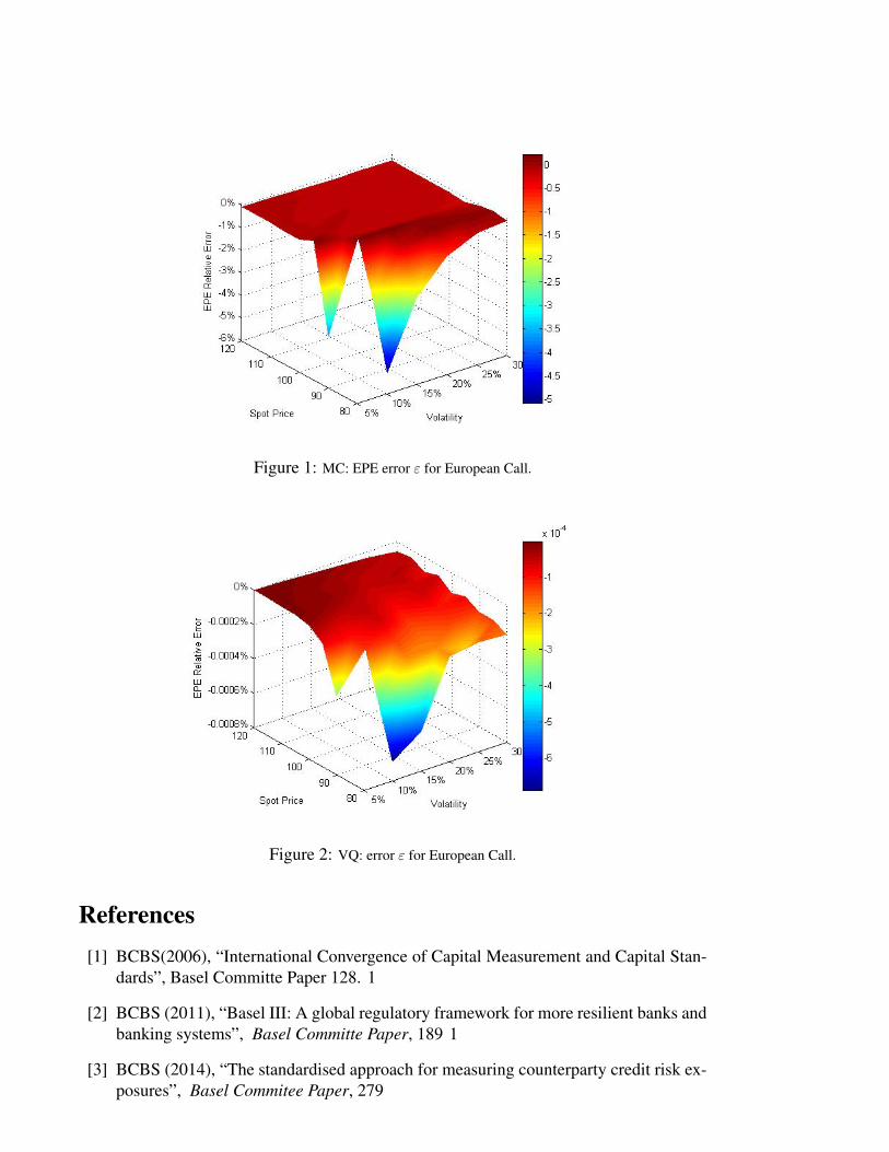
Figure 1: MC: EPE error ε for European Call.

Figure 2: VQ: error ε for European Call.

References[1] BCBS(2006), “International Convergence of Capital Measurement and Capital Stan-

dards”, Basel Committe Paper 128. 1

[2] BCBS (2011), “Basel III: A global regulatory framework for more resilient banks andbanking systems”, Basel Committe Paper, 189 1

[3] BCBS (2014), “The standardised approach for measuring counterparty credit risk ex-posures”, Basel Commitee Paper, 279

18

[4] Bally V., Pagı¿œs G., Printemps J. (2010), “A quantization tree method for pricingand hedging multi-dimensional American options”, Working Paper 3

[5] Black F., Scholes M. (1973), The Pricing of Options and Corporate Liabilities Jour-nal of Political Economy 81 (3), 637–654. 4

[6] Bucklew, J.A. and Wise, G.L. (1982) Multidimensional asymptotic quanti- zationtheory with rth power distortion, IEEE Trans. Inform. Theory, Vol.28, NO.2 3

[7] Caflisch, R.E. and Morokoff, W.J., (1995) Quasi-Monte Carlo integration, J. Comput.Phys. Vol.122 , no. 2 5.2

[8] Castagna A. (2012), “Fast computing in the CCR and CVA measurement”, IASONALGO, Working Paper. 3

[9] Cesari G. et al. (2009), Modeling, Pricing and Hedging Counterparty Credit Expo-sure, Springer Finance Editor. 1

[10] Dupire B. (1994), “Pricing with a smile”, Risk, , January, 18-20. 4

[11] Gersho A., Gray R. (1982), “IEEE on Information Theory, Special Issue on Quanti-zation”, No.28. 3

[12] Hagan P. et al (2002), “Managing Smile Risk”, Wilmott Magazine 4

[13] Heston S. (1993), A Closed-Form Solution for Options with Stochastic Volatility withApplications to Bond and Currency Options The Review of Financial Studies 6 (2),327–,343. 4

[14] IFRS (2013), “IFRS 13 Fair Value Measurement”, IFRS Technical Paper 1

[15] A.Mikes, (2013), The Appeal of the Appropriate: Accounting, Risk Management,and the Competition for the Supply of Control Systems, Harward Business School -working papers, No.12, Vol.115 1

[16] Pagı¿œs G., Printemps J., Pham H. (2004), “Optimal quantization methods and ap-plications to numerical problems in finance”, Handbook on Numerical Methods inFinance, Birkhı¿œuser, 253-298. 3, 3, 3, 3, 4

[17] Pagı¿œs G., Luschgy H. (2006), “Functional quantization of a class of Browniandiffusions: A constructive approach”, Stochastic processes and their Applications,Elsevier, No.116, 310-336. 3, 8

[18] Pagı¿œs G., Wilbertz B. (2012), “Intrinsic stationarity for vector quantization: Foun-dation of dual quantization”, SIAM Journal on Numerical Analysis, 747-780. 3

[19] Pagı¿œs G., Wilbertz B. (2011), “GPGPUs in computational finance: Massive parallelcomputing for American style options”, Working paper. 4

[20] Pykhtin M., Zhu S. (2007), “A Guide to Modelling Counterparty Credit Risk”, GARPpublication. 2

19

[21] Sellami, A. (2005) Mı¿œthodes de quantification optimale pour le filtrage et applica-tions ı¿œ la finance, Applied mathematics: Universitı¿œ Paris Dauphine. 3

[22] Shreve, S., (2004) Stochastic Calculus for Finance II. Continuous time models,Springer Finance series 2, 5, 5.2

[23] Zador, P.L. (1963), Development and evaluation of procedures for quantizing multi-variate distributions, Ph.D. dissertation, Stanford Univ. (USA). 3

[24] Zador, P.L. (1982), Asymptotic quantization error of continuous signals and the quan-tization dimension. IEEE Trans. Inform. Theory, Vol.28, No.2.

3

20