A Quantitative Comparative Study of Analytical and Iterative Reconstruction Techniques

Shrinivas D Desai & Dr Linganagouda Kulkarni

International Journal Of Image Processing (IJIP), Volume (4): Issue (4) 307

A Quantitative Comparative Study of Analytical and Iterative Reconstruction Techniques

Shrinivas D Desai [email protected] Assistant Professor, Dept of ISE B V B College of Engineering & Technology HUBLI – 580031 Karnataka,India

Dr Linganagouda Kulkarni [email protected] JPNES Group of Institutions – School of Engineering / School of Pharmacy MEHABUBNAGAR Andra Pradesh, India

Abstract

Measurement of visual quality is of great importance in the field of medical image applications such as X-ray tomography. In applications such as CT and MRI scanning, most of the time quality of reconstructed image is assessed qualitatively by radiologist or domain experts which are purely subjective evaluation [1]. However quantitative analysis or machine evaluation of reconstructed image appeals more to medical practitioners and normally aids the diagnosing of disease. Hence there is immense need for parameters which quantitatively measures the quality of reconstructed images. This paper proposes six image quality measurement parameters (IQM) and comparison of both qualitative ratings and proposed quantitative method for images reconstructed in CT by analytical and iterative techniques [2] is presented here. Projections (parallel beam type) for the image reconstruction are calculated analytically by defining Shepp logan phantom head model with coverage angle ranging from 0 to ±180o with rotational increment of 2o to 10o. For iterative reconstruction coverage angle of ±90o, iteration up to 10 is used. The original image is grayscale image of size 128 X 128. Experiment results reveal very close similarity among assessment done qualitatively with those of assessment done quantitatively. Hence the proposed six quality measurement parameters appear to be effective for assessing the quality of reconstructed image in CT applications. Keywords: Reconstruction algorithm, Simple-Back projection algorithm (SBP), Filter-Back projection algorithm (FBP), Algebraic Reconstruction Technique algorithm (ART), Image quality, coverage angle, Computed tomography (CT).



1. INTRODUCTION For applications such as CT and MRI in which images are to be viewed by human beings, the ultimate method of quantifying visual image quality is through subjective evaluation [4]. In practice, however, subjective evaluation is usually too inconvenient; require expertise, time-consuming and expensive. The majority of the proposed perceptual quality assessment models have followed a strategy of modifying the MSE measure so that errors are penalized in accordance with their visibility. The most reported objective method for image quality measurement parameters are Peak Signal to Noise Ratio, Human Visual System [3], Picture Quality Scale [5, 6], Noise Quality Measure [7], Fuzzy [8], Multi-scale Structural Similarity Index Metric [9], Information fidelity criterion [10], and Visual information fidelity [11] which works with luminance only. While IQM which works on color images are Sarnoff model [12, 13], BSDM [14], Universal image quality index [15] and DC tune [16]. The resent reported IQM for structural similarity is MSSIM index, which is combination of three comparisons: luminance, contrast and structure [4]. Quantifying differential qualities using various dissimilar metric is yet another IQM proposed to discriminate reconstructed image. Literature presents six dissimilarity metrics namely Euclidean distance, Manhattan distance, Canberra distance, Bray-Curtis distance, Squared Chord distance and Chi-Squared distance to identify the metric that provide better classification between the reconstructed and original image [17]. In CT applications, where images are grayscale, the image quality measurement doesn’t necessarily depend on luminance or color. In this regard we propose six IQM parameters to objectively measure gray scale reconstructed image which are generated in CT applications using analytical and iterative techniques.

2. METHOD The following section deals with different methods available for reconstruction of image from projections.

2.1 Reconstruction:

Given the sinogram p(r, θ) we want to recover the object described in (x, y) coordinates. Basically it works by subsequently “smearing” the acquired p(r, θ) across a film plate. This is simple back projection [18]

∫Π

+==

0

),sin.cos.()},({),( θθθθθ dyxprpByxb -- 2.1

2.2 Filtered Back projection:

We need a way to equalize the contributions of all frequencies in the FT’s polar grid, this can be done by multiplying each P(k,θ) by a ramp function. This way the magnitudes of the existing higher-frequency samples in each projection are scaled up to compensate for their lower amount. The ramp is the appropriate scaling function since the sample density decreases linearly towards the FT’s periphery [18]. Filtered back projection is given as

θθ ddkkkPyxf ekri

)..),((),(2

0

Π

Π ∞

∞−

∫ ∫= -- 2.2

where P(k, θ) is 1 D Fourier transform of p(r, θ), multiplying with |k| gives ramp filtering, integrating the expression from ∞ to - ∞ gives inverse 1D Fourier transform, and integrating from 0 to П gives filtered back projection for all angles.



2.3 Algebraic Reconstruction: An entirely different approach for Tomographic imaging consists of assuming that the cross section consists of an array of unknowns and the setting up algebraic equations for the unknowns in terms of the measured projection data. All algebraic reconstruction technique methods are iterative procedures. There are two approaches for reconstructing the image using iterative technique [19]. In first approach the process starts with an initial estimate and tries to push the estimate closer to the true solution. Instead of back-projecting the average ray value, the projections corresponding to the current estimate are compared with the measured projections. The result of the comparison is used to modify the current estimate, thereby creating a new estimate. In the second approach ART pose the reconstruction problem as a set of simultaneous equations. Here a square grid is assumed to superimpose over the unknown cross-section image. Image values are assumed to be constant within each cell of the grid. The set of linear equation for each ray is then formed.

MipfwN

j

ijij ,...,2,1,1

==∑=

-- 2.3

where pi are projection data along the i

th ray, wij the fraction area of j image cell intercepted by i

th

ray, fj are the values of the reconstruction grid element (pixel) , M is the total number of rays (in all the projection) and N is the number of grid cell. For a large values of M and N there exist an iterative methods for solving (2.3), which is One iteration step the Kaczmarz method. The Kaczmarz method, based on the work of the Polish mathematician Stefan Kaczmarz [20], is a method for solving linear systems of equations Ax = b. It was rediscovered in the field of image reconstruction from projections where it is called the Algebraic Reconstruction Technique (ART) [21].

Wp

ff kjN

i

kl

i

kk

i

j

i

j

W

fw..

1

2

1)1()(

∑=

−

− −+= λ -- 2.4

Where =fi

j

)(

New pixel value, =−

fi

j

)1(

Old pixel value, =λ Relaxation parameter,

=−−1i

kk

fwp The difference, =∑=

N

i

klW1

2 Normalizing the difference, =W kj

Weighting the

correction Equation (2.4) is the well-known algebraic reconstruction technique (ART) where the second term on the left is the correction factor for ray i

th. Apparently, equation 2.4 is used to update the j

th pixel

on every ray equation.

3. EXPERIMENTS Figure. 3.1 shows the 2D shepp logan phantom head model used in our study. It is constructed from basic ellipsoids as per standard [24], which allows us to calculate their projections analytically [22]. The size of the model defined here is 128 X 128, grayscale image.



Figure 3.1 2D Shepp Logan phantom head model

Figures 3.2 a, b, c are the standard medical images of brain, abdomen and breast are used in our study [23]. Projections are calculated mathematically and reconstructed using SBP, FBP and ART techniques.

(a) (b) (c)

Figure 3.2 Standard medical image (a) Brain (b) Abdomen (c) Breast

3.1 Quality measurement parameters: The quality of reconstructed image is quantified by six quality measurement parameters as listed below. 1) Mean Square Error (MSE): Mean square error is the sum over all squared value differences divided by image size. It’s a measure between the original image and the reconstructed image

∑∑==

−=

N

k

M

j

yxIyxIMN

MSE1

2'

1

)],(),([(1

--3.1

Where I(x,y) is the original image, I'(x,y) is the reconstructed image, and M,N are the dimensions of the images. 2) Peak signal to noise ratio (PSNR): is a measure of the peak error

=

MSEPSNR

255log10 -- 3.2

A lower value for MSE means lesser error, and as seen from the inverse relation between the MSE and PSNR, this translates to a high value of PSNR. Logically, a higher value of PSNR is good because it means that the ratio of Signal to Noise is higher. Here, the 'signal' is the original image, and the 'noise' is the error in reconstruction 3) Normalized Cross-Correlation (NCC) : Normalized Cross-Correlation is one of the methods used for template matching, a process used for finding incidences of a pattern or object within an image

∑∑∑∑====

−=

N

k

M

j

N

k

M

j

yxIyxIyxINCC1

2

1

2'

11

),((/)),(),(( -- 3.3



4) Structural Content (SC) : Structural content establishes the degree to which an image in the collection matches. It’s the measure of image similarity based on small regions of the images containing significant low level structural information. The more the number of such regions common to both images, the more similar they are considered.

∑ ∑∑∑= = ==

=

N

k

M

j

N

k

M

j

yxIyxISC1 1 1

2'2

1

),(),(( -- 3.4

5) Maximum Difference (MD): It’s the variation of the method of paired comparisons.

−= kkMaxMD xx jj

,,'

-- 3.5

6) Normalized Absolute Error (NAE): It’s the numerical difference between the original and reconstructed image.

∑ ∑∑∑= = ==

−=

N

k

M

j

N

kjjj

M

j

kkkNAE xxx1 1 1

'

1

,,, -- 3.6

4. RESULTS & DISCUSSION Comparison of reconstruction techniques such as SBP, FBP (analytical), & ART (iterative) with respect to quality of reconstructed image is presented in this section. Projections calculated analytically are assumed for parallel projection data and the center of rotation as the center point of the projections. Number of projections and angular range: The reconstruction discrepancy such as MSE was calculated for 18, 24, 36, and 72 projections, taken over angular ranges of 0 to ±180

o with

incremental ranging from 2o to 10

o. The original image is of size 128 X 128. It was found that, for

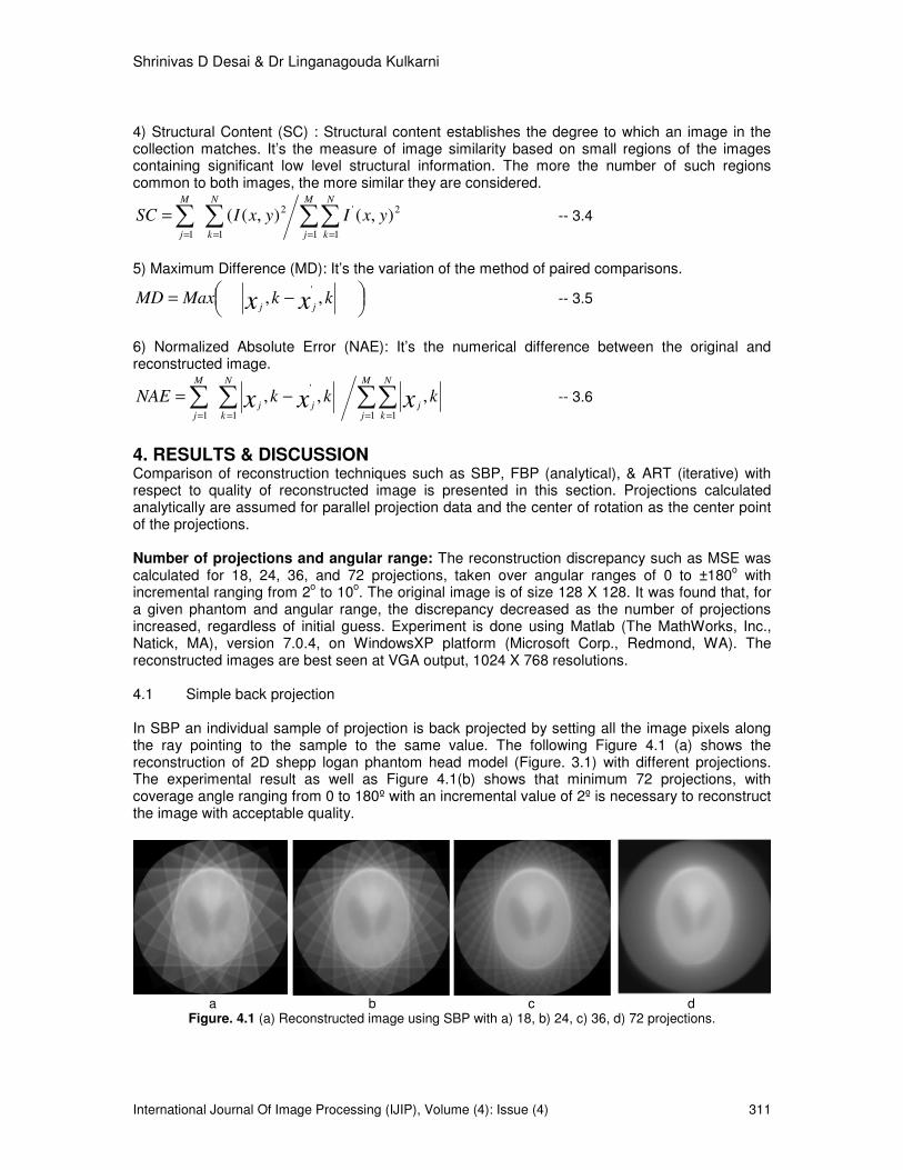
a given phantom and angular range, the discrepancy decreased as the number of projections increased, regardless of initial guess. Experiment is done using Matlab (The MathWorks, Inc., Natick, MA), version 7.0.4, on WindowsXP platform (Microsoft Corp., Redmond, WA). The reconstructed images are best seen at VGA output, 1024 X 768 resolutions. 4.1 Simple back projection In SBP an individual sample of projection is back projected by setting all the image pixels along the ray pointing to the sample to the same value. The following Figure 4.1 (a) shows the reconstruction of 2D shepp logan phantom head model (Figure. 3.1) with different projections. The experimental result as well as Figure 4.1(b) shows that minimum 72 projections, with coverage angle ranging from 0 to 180º with an incremental value of 2º is necessary to reconstruct the image with acceptable quality.

a b c d

Figure. 4.1 (a) Reconstructed image using SBP with a) 18, b) 24, c) 36, d) 72 projections.



Mean square error in SBP

0

5000

10000

15000

20000

25000

0 20 40 60 80 100 120

ProjectionsM

ean

sq

uare

err

or

Figure 4.1 (b) Mean square error v/s projections for SBP

SBP can be referred to as a “brute force” technique. It’s a simple and non effective method of obtaining an approximate reconstruction from multiple projections, and this technique generates star or spoke artifact. Image padding is necessary so that pixel values at borders are retained even after rotating the P-H model. Figure 4.1 (b) clearly reveals that the quality of reconstructed image increases as number of projection increases, MSE settles down from 72 projections. However the reconstructed image appears to be very blurry. 4.2 Filtered Back projection: In FBP each view is filtered before the back projection to counteract the blurring effect. That is, each of the one-dimensional views is convolved with a one-dimensional filter kernel to create a set of filtered views. These filtered views are then back projected to provide the reconstructed image, a close approximation to the correct image. In fact, the image produced by filtered back projection is identical to the correct image when there are an infinite number of views and an infinite number of points per view. The Figure 4.2 (a) shows reconstruction of phantom head model by FBP with coverage angle ranging from 0 to 180º with an incremental value of 10º to 2º.

a b c d

Figure 4.2 (a) Reconstructed image using FBP with a) 18, b) 24, c) 36, d) 72 projections.



Mean square error for FBP

0

2000

4000

6000

8000

10000

12000

0 10 20 30 40 50 60

Projections

Mean

sq

uare

err

or

Figure 4.2 (b) Mean square error v/s projections for FBP

Figure 4.2 (b) clearly reveals that the quality of reconstructed image increases as number of projection increases, the MSE of the reconstructed image remains constant after 36 projections. This algorithm requires minimum of 36 projections with rotational increment of 5

0 to display

acceptable reconstructed image. It is the most common method of removing the star artifact which is normally generated in SBP by using various filters. FBP algorithm used for reconstruction of image from its projections is found to be fast and efficient with large number of projections. It is fast and efficient with large number of projections. We can say that it is direct inversion of the projection formula. But here qquantitative imaging is difficult. FBP has become more popular and commercialized in nuclear medicine.

4.3 Algebraic Reconstruction technique:

In ART all the pixels in the image array is set to some arbitrary value. In experiment it is set to average value of the phantom head model. An iterative procedure is then used to gradually change the image array to correspond to the profiles. Using first approach after the first complete iteration cycle, there will still be an error between the ray sums and the measured values. This is because the changes made for any one measurement disrupts all the previous corrections made. The idea is that the errors become smaller with repeated iterations until the reconstructed image converges to the proper solution. The Figure 4.3 shows reconstruction of phantom head model with “smart” initial guess, coverage angle 0 to 90º, increment of 5º, iterations from 3 to 8.

a b c d

Figure 4.3 Reconstructed image with ART: a) θ = 5, Iteration=3 b) θ = 5, Iteration=4 c) θ = 5, Iteration=6 d) θ = 5, Iteration=8

The principle of ART is to find a solution by successive estimates. The projections corresponding to the current estimate are compared with the measured projections. The result of the comparison is used to modify the current estimate, thereby creating a new estimate. Corrections are carried out either as addition of differences or multiplication by quotients between measured and estimated projections. Figure 4.4 (a) and (b) shows the difference between reconstructed and original image by drawing NAE versus iterations for difference correction and multiplicative corrections respectively.



-25

-20

-15

-10

-5

0

5

10

15

20

0 10 20 30 40 50

Iterations

Dif

fere

nce

-5

-4

-3

-2

-1

0

1

2

3

4

5

0 10 20 30 40 50

Iterations

Dif

fere

nce

a b

Figure 4.4 NAE versus iteration a) difference correction b) multiplicative corrections. In ART obviously, the errors of phantom obtained from the algebraic formulations are less than that of the filtered back projection; the star artifact appearing in image reconstructed from the filtered back projection is disappeared with the method of algebraic formulation. However, the algebraic formulations take more time to complete the process than does the filtered back projection. The following table shows quality of reconstructed image measured by six quality measurement parameters. Table 4.1(a) shows the quality measurement of reconstructed by varying number of projections, & keeping common coverage angle, while Table 4.1(b) shows the quality measurement by varying coverage angle, & keeping common number of projections.

Coverage angle: ± 90◦ Number of projections: 72


Image Quality Measurement

SBP FBP ART SBP FBP ART

MSE 4938.6 572.7858 2586.4 2532.4 1275.6 286.25

PSNR 11.1947 20.5509 14.0039 5.689 7.56 10.57

NCC 1.0113 0.9949 1.0039 0.58 0.57 0.4612

SC 0.8773 0.9984 0.9356 0.48 0.47 0.4824 MD 115 255 143 56 75 129

NAE 0.2119 0.0262 0.1534 0.125 0.078 0.0112 Table 4.1 (a) : Image quality measurement by varying number of projections keeping fixed coverage angle.

The experiments revealed major observations; as the number of projections within a given angular range was increased, the quality of reconstructed image appeared better. Regarding the angular range, it was found that the discrepancy decreased with increasing angular range.



Image Quality Measurement

SBP FBP ART SBP FBP ART

MSE 2532.4 1275.6 286.25 1526.5 624.25 135.2

PSNR 5.689 7.56 10.57 2.589 3.251 5.26

NCC 0.58 0.57 0.4612 0.24 0.245 0.218

SC 0.48 0.47 0.4824 0.18 0.214 0.26

MD 56 75 129 29 32 72

NAE 0.125 0.078 0.0112 0.08 0.026 0.059

Table 4.1 (b) : Image quality measurement by varying coverage angle keeping fixed number of projections



Table 4.1 (c) shows Image quality measurement for Figure 3.2 a, b, c reconstructed from SBP, FBP, ART. The experiment reveals the fact that FBP effectively eliminates Star artifacts created by SBP. ART performs better even at limited views, and has better noise tolerance.

MSE PSNR NCC SC MD NAE

Model Technique

Brain SBP 1646.2 3.731567 0.3371 0.292433 38.33333 0.070633 FBP 190.9286 6.8503 0.331633 0.3328 85 0.008733 ART 862.1333 4.667967 0.334633 0.311867 47.66667 0.051133

Abdomen SBP 1975.44 4.47788 0.40452 0.35092 46 0.08476 FBP 229.1143 8.22036 0.39796 0.39936 102 0.01048 ART 1034.56 5.60156 0.40156 0.37424 57.2 0.06136

Breast SBP 3292.4 7.463133 0.6742 0.584867 76.66667 0.141267 FBP 381.8572 13.7006 0.663267 0.6656 170 0.017467 ART 1724.267 9.335933 0.669267 0.623733 95.33333 0.102267

Table 4.1 (c) Image quality measurement for Figure 3.2 a, b, c reconstructed from SBP, FBP, ART.

Table 4.2 shows the reconstruction time for Figure 3.1 Shepp logan phantom head model using analytical & iterative techniques.

Number of projections

Technique 18 24 36 72 SBP 5.24 10.26 15.24 20.72 FBP 0.75 1.23 1.95 2.38 ART 5.42 11.24 16.58 21.24

Table 4.2: Reconstruction time* for Figure 3.1 for different number of projections. Time in seconds.

ART requires more time compared to others for reconstruction, while FBP requires least. However, the SBP take more time to complete the process than does the FBP, but less as compared to ART. Table 4.3 shows the reconstruction time for three standard medical images brain, abdomen, and breast with different number of projections

Technique Brain Abdomen Breast Number of Projections 36 72 36 72 36 72

SBP 10.34 20.35 10.45 20.36 9.96 19.94 FBP 0.95 2.16 0.98 2.15 0.86 2.03 ART 11.24 23.15 11.28 24.16 10.56 20.56

Table 4.3: Reconstruction time* for Figure 3.2 a, b, c for different number of projections. Time in

seconds

* Results obtained using Matlab (The MathWorks, Inc., Natick, MA), version 7.0.4, under the Window XP operating system (Microsoft Corp., Redmond, WA), on Intel Pentium Core2 Duo, CPU 2.80GHz, 1GB RAM.



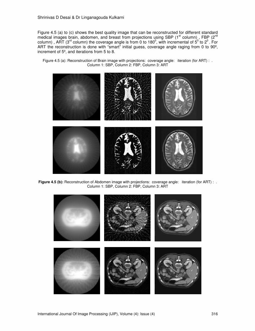
Figure 4.5 (a) to (c) shows the best quality image that can be reconstructed for different standard medical images brain, abdomen, and breast from projections using SBP (1

st column) , FBP (2

nd

column) , ART (3rd

column) the coverage angle is from 0 to 1800, with incremental of 5

0 to 2

0 . For

ART the reconstruction is done with “smart” initial guess, coverage angle raging from 0 to 90º, increment of 5º, and iterations from 5 to 8.

Figure 4.5 (a): Reconstruction of Brain image with projections: coverage angle: iteration (for ART) : .

Column 1: SBP, Column 2: FBP, Column 3: ART

Figure 4.5 (b): Reconstruction of Abdomen image with projections: coverage angle: iteration (for ART) : .

Column 1: SBP, Column 2: FBP, Column 3: ART



Figure 4.5 (c): Reconstruction of Breast image with projections: coverage angle: iteration (for ART) : . Column 1: SBP, Column 2: FBP, Column 3: ART

5.CONCLUSION The quantitative comparative study of analytical and iterative techniques for image reconstruction from projections for computed tomography revealed a case of diminishing returns, which are concluded as below. In this work, objective measurement by Mean Square Error, Peak signal to noise ratio, Normalized Cross-Correlation, Structural Content, Maximum Difference and Normalized Absolute Error led to an ability to subjectively judge the reconstructed image quality. The major problem with SBP reconstruction is that it leaves “extra” counts on the image because of which reconstructed image appears severe blur nature or has “Star” like pattern. In case of FBP; it removes the star artefact produced in SBP, and by using Ram-Lak with Hamming / Butterworth filter we can simultaneously reduce high-frequency components (containing much noise) and low-frequency component (containing blur). The image produced by the ART technique has poor density resolution, acceptable spatial resolution, but requires large computational time. The spoke artifact appearing in image reconstructed from the filtered back projection is disappeared in algebraic formulation; it possesses better noise tolerance. These subjective evaluations are in close with objective evaluation done using six IQM. From the experiments, we shall conclude that proposed six IQM all together is reliable and practical to measure the quality of reconstructed images for CT applications.



6.REFERENCES

1. H. R. Sheikh, M. F. Sabir, A. C. Bovik. “A Statistical Evaluation of Recent Full Reference Image Quality Assessment Algorithms”. IEEE Transactions on Image Processing, 15(11): 2006

2. P. P. Bruyant. “Analytic and Iterative Reconstruction Algorithms in SPECT”. Journal of Nuclear Medicine, by Society of Nuclear Medicine, 43(10): 1343-1358, 2002

3. N. Yamsang and S. Udomhunsakul. “Image Quality Scale (IQS) for Compressed Images Quality Measurement”. Proceedings of the International Multi Conference of Engineers and Computer Scientists 2009 Vol I IMECS 2009, Hong Kong, 2009

4. Z. Wang, A. C. Bovik, H. R. Sheikh, E. P. Simoncelli. “Image Quality Assessment: From Error Visibility to Structural Similarity”, IEEE Transactions On Image Processing, 13(4): 2004

5. M. Miyahara, K. Kotani, V. R. Algazi,. “Objective Picture Quality Scale (PQS) for image coding,” IEEE Trans. Commun., 46(9), 1215–1225,1998

6. CIPIC PQS ver. 1.0, [Online]. Available at: http://msp.cipic.ucdavis.edurestes/ftp/cipic/code/pqs,

7. N. Damera-Venkata, T. D. Kite, W. S. Geisler, B. L. Evans, A.C. Bovik. “Image quality assessment based on a degradation model”. IEEE Trans. Image Process., 4(4): 636–650, 2000

8. D. V. Weken, M. Nachtegael, E. E. Kerre. “Using similarity measures and homogeneity for the comparison of images”. Image Vis. Comput., 22: 695–702, 2004

9. Z. Wang, E. P. Simoncelli, and A. C. Bovik, “Multi-scale structural similarity for image quality assessment,” presented at the IEEE Asilomar Conf. Signals, Systems, and Computers, 2003

10. H. R. Sheikh, A. C. Bovik, G. de Veciana. “An information fidelity criterion for image quality assessment using natural scene statistics”. IEEE Trans. Image Process., 14(12): 2117–2128, 2005

11. H. R. Sheikh, A. C. Bovik. “Image information and visual quality”. IEEE Trans. Image Process., 15(2), 430–444, 2006

12. JNDmetrix Technology Sarnoff Corp., evaluation Version, 2003 [Online]. Available at : http://www.sarnoff.com/products-services/video-vision/jndmetrix/ downloads.asp

13. J. Lubin. “A visual discrimination mode for image system design and evaluation”. in Visual Models for Target Detection and Recognition (E. Peli, ed.), Singapore: World Scientific Publishers pp. 245–283, (1995)

14. I. Avcibas¸, B. Sankur, K. Sayood. “Statistical evaluation of image quality measures”. J. Electron. Imag., 11(2): 206–23, 2002.

15. Z. Wang, A. C. Bovik. “A universal image quality index”. IEEE Signal Processing Letters, 9: 81–84, 2002.

16. A. B. Watson. “DCTune: A technique for visual optimization of DCT quantization matrices for individual images”. Soc. Inf. Display Dig. Tech. Papers, vol. XXIV, pp. 946–949, (1993)

17. K. B. Raja, M.Madheswaran, K.Thyagarajah. “Quantitative and Qualitative Evaluation of US Kidney Images for Disorder Classification using Multi-Scale Differential Features”. ICGST-BIME Journal, 7(1): 2007



18. K. Mueller and R. Yagel. “On the Use of Graphics Hardware to Accelerate Algebraic Reconstruction Methods”. Presented at the SPIE Medical Imaging Conference Physics of Medical Imaging, San Diego, 1999

19. A.M. Ali, Z. Melegy , M. Morsy , R.M. Megahid , T. Bucherl , E.H. Lehmann. “Image reconstruction techniques using projection data from transmission method”. Annals of Nuclear Energy, 31: 1415–1428, Elsevier Ltd, 2004

20. Kaczmarz, S. „Angenäherte Auflösung von Systemen linearer Gleichungen“. Bulletin International de l'Academie Polonaise des Sciences et des Lettres, series A, 35 :335-357, 1937

21. Gordon, R., R. Bender, G.T. Herman. “Algebraic reconstruction techniques (ART) for threedimensional electron microscopy and x- ray photography”. Journal of Theoretical Biology, 29:471-481, 1970.

22. A. K. Jain. “Fundamentals of Digital Image Processing”, Prentice – Hall of India, 1 - Edition, pp.431 – 470, (1989)

23. Medical Image Samples Sebastien Barre, Online image database, “Archive of DICOM images” [online] Available at:http://www.barre.nom.fr/medical/samples/

24. S. D. Desai. “Reconstruction of image from projections-an application to MRI & CT Scanning”. In proceedings of International conference ICSCI-2005

A Quantitative Comparative Study of Analytical and Iterative Reconstruction Techniques

Education

Transcript of A Quantitative Comparative Study of Analytical and Iterative Reconstruction Techniques