
A Probabilistic Polynomial-time Calculus For Analysis of ...
31
Electronic Notes in Theoretical Computer Science 45 (2001) URL: http://www.elsevier.nl/locate/entcs/volume45.html 31 pages A Probabilistic Polynomial-time Calculus For Analysis of Cryptographic Protocols (Preliminary Report) J. Mitchell 1,3,4 Computer Science Department, Stanford University, Stanford, CA 94305 USA A. Ramanathan 1 Computer Science Department, Stanford University, Stanford, CA 94305 USA A. Scedrov 1,2,5 Mathematics Department, University of Pennsylvania, Philadelphia PA 19104-6395 USA V. Teague 1,6 Computer Science Department, Stanford University, Stanford, CA 94305 USA Abstract We describe properties of a process calculus that has been developed for the pur- pose of analyzing security protocols. The process calculus is a restricted form of π-calculus, with bounded replication and probabilistic polynomial-time expressions allowed in messages and boolean tests. In order to avoid problems expressing se- curity in the presence of nondeterminism, messages are scheduled probabilistically instead of nondeterministically. We prove that evaluation may be completed in probabilistic polynomial time and develop properties of a form of asymptotic proto- col equivalence that allows security to be specified using observational equivalence, a standard relation from programming language theory that involves quantifying over possible environments that might interact with the protocol. We also relate process equivalence to cryptographic concepts such as pseudo-random number generators and polynomial-time statistical tests. c 2001 Published by Elsevier Science B. V.
Transcript of A Probabilistic Polynomial-time Calculus For Analysis of ...
Electronic Notes in Theoretical Computer Science 45 (2001)URL: http://www.elsevier.nl/locate/entcs/volume45.html 31 pages
A Probabilistic Polynomial-time CalculusFor Analysis of Cryptographic Protocols
(Preliminary Report)
J. Mitchell 1,3,4
Computer Science Department, Stanford University, Stanford, CA 94305 USA
A. Ramanathan 1
Computer Science Department, Stanford University, Stanford, CA 94305 USA
A. Scedrov 1,2,5
Mathematics Department, University of Pennsylvania, Philadelphia PA19104-6395 USA
V. Teague 1,6
Computer Science Department, Stanford University, Stanford, CA 94305 USA
Abstract
We describe properties of a process calculus that has been developed for the pur-pose of analyzing security protocols. The process calculus is a restricted form ofπ-calculus, with bounded replication and probabilistic polynomial-time expressionsallowed in messages and boolean tests. In order to avoid problems expressing se-curity in the presence of nondeterminism, messages are scheduled probabilisticallyinstead of nondeterministically. We prove that evaluation may be completed inprobabilistic polynomial time and develop properties of a form of asymptotic proto-col equivalence that allows security to be specified using observational equivalence, astandard relation from programming language theory that involves quantifying overpossible environments that might interact with the protocol. We also relate processequivalence to cryptographic concepts such as pseudo-random number generatorsand polynomial-time statistical tests.
c©2001 Published by Elsevier Science B. V.
Mitchell, Ramanathan, Scedrov, and Teague
1 Introduction
A variety of methods are used for analyzing and reasoning about security pro-tocols. The main systematic or formal approaches include specialized logicssuch as BAN logic [8,13], special-purpose tools designed for cryptographic pro-tocol analysis [20], and theorem proving [32,31] and model-checking methodsusing several general purpose tools described in [24,26,29,34,35]. Althoughthese approaches differ in significant ways, all reflect the same basic assump-tions about the way an adversary may interact with the protocol or attempt todecrypt encrypted messages. In the common model, largely derived from [12]and suggestions found in [30] (see, e.g., [10]), a protocol adversary is allowedto nondeterministically choose among possible actions. This is a convenientidealization, intended to give the adversary a chance to find an attack if thereis one. In the presence of nondeterminism, however, the set of messages anadversary may use to interfere with a protocol must be restricted severely.Although the Dolev-Yao-style assumptions make protocol analysis tractable,they also make it possible to “verify” protocols that are in fact susceptibleto simple attacks that lie outside the adversary model. Another limitation isthat a deterministic or nondeterministic setting does not allow us to analyzeprobabilistic protocols.
In this paper we describe some general concepts in security protocol anal-ysis, mention some of the competing approaches, and describe some technicalproperties of a process calculus that was proposed earlier in [23,22] as the ba-sis for a form of protocol analysis that is formal, yet closer in foundations tothe mathematical setting of modern cryptography. The framework relies ona language for defining communicating polynomial-time processes [28]. Thereason we restrict processes to probabilistic polynomial time is so that we canreason about the security of protocols by quantifying over all “adversarial”processes definable in the language. In effect, establishing a bound on therunning time of an adversary allows us to relax the simplifying assumptions.Specifically, it is possible to consider adversaries that might send randomlychosen messages, or perform sophisticated (yet probabilistic polynomial-time)computation to derive an attack from messages it overhears on the network.An important aspect of our framework is that we can analyze probabilistic aswell as deterministic encryption functions and protocols. Without a proba-bilistic framework, it would not be possible to analyze an encryption functionsuch as ElGamal [14], for which a single plaintext may have more than one
1 Partially supported by DoD MURI “Semantic Consistency in Information Exchange”through ONR Grant N00014-97-1-0505.2 Additional support by OSD/ONR CIP/SW URI “Software Quality and InfrastructureProtection for Diffuse Computing” through ONR Grant N00014-01-1-0795.3 Additional support from DARPA Contract N66001-00-C-8015.4 Additional support from NSF CCR-9629754.5 Additional support from NSF Grants CCR-9800785 and CCR-0098096.6 Partially supported by Stanford Graduate Fellowship.
2
Mitchell, Ramanathan, Scedrov, and Teague
ciphertext.
Some of the basic ideas of this work are outlined in [23], with the termlanguage presented in [28] and further example protocols considered in [22].The closest technical precursor is the Abadi and Gordon spi-calculus [3,2]which uses observational equivalence and channel abstraction but does notinvolve probability or computational complexity bounds; subsequent relatedwork is cited in [1], for example. Prior work on CSP and security protocols,e.g., [34,35], also uses process calculus and security specifications in the formof equivalence or related approximation orderings on processes.
Although our main long-term objective is to base protocol analysis onstandard cryptographic assumptions, this framework may also shed new lighton basic questions in cryptography. In particular, the characterization of “se-cure” encryption function, for use in protocols, does not appear to have beencompletely settled. While the definition of semantic security in [18] appearsto have been accepted, there are stronger notions such as non-malleability [11]that are more appropriate to protocol analysis. In a sense, the difference isthat semantic security is natural for the single transmission of an encryptedmessage, while non-malleability accounts for vulnerabilities that may arise inmore complex protocols. Our framework provides a setting for working back-wards from security properties of a protocol to derive necessary propertiesof underlying encryption primitives. While we freely admit that much moreneeds to be done to produce a systematic analysis method, we believe thata foundational setting for protocol analysis that incorporates probability andcomplexity restrictions has much to offer in the future.
2 Preliminaries
2.1 Probabilistic Functions
Definition 2.1 We define a probabilistic function F on the sets X, Y as afunction F : X × Y → [0, 1] that satisfies the following condition:
∀x ∈ X :∑y∈Y
F(x, y) ≤ 1 (1)
For some x ∈ X, y ∈ Y , if F(x, y) = p, we say that F takes on the value y atx with probability p or that F(x) = y with probability p.
2.2 Composition of Probabilistic Functions
Definition 2.2 We define the composition F : X × Z → [0, 1] of two proba-bilistic functions F1 : X×Y → [0, 1] and F2 : Y ×Z → [0, 1] as a probabilisticfunction that satisfies the following condition:
∀x ∈ X.∀z ∈ Z : F(x, z) =∑y∈Y
F1(x, y) · F2(y, z) (2)
3
Mitchell, Ramanathan, Scedrov, and Teague
We write the composition of F1 and F2 as F2 ◦ F1.
Lemma 2.3 Given two probabilistic functions F1 : X × Y → [0, 1] and F2 :Y ×Z → [0, 1], the composition F2 ◦F1 = F : X×Z → [0, 1] is a probabilisticfunction, i.e., it satisfies the condition ∀x ∈ X :
∑z∈Z F(x, z) ≤ 1.
Proof. For any fixed x ∈ X:
∑z∈Z
F(x, z) =∑z∈Z
∑y∈Y
F1(x, y) · F2(y, z) by defn. 2.2
=∑y∈Y
F1(x, y) ·∑z∈Z
F2(y, z) factoring
≤ 1 by defn. 2.1
Hence, composition is a probabilistic function. 2
2.3 Terminology
In what follows, P denotes a process, T denotes a term, p(x) denotes oneof an infinity of bandwidth polynomials such that ∀a ∈ N : p(a) ≥ 0. cp(x)
denotes one of a countable infinity Cq(x) of channel names associated with thepolynomial p(x) in such a way that no channel name is associated with morethan one polynomial.
There is a special security parameter, n, that can appear in terms (sec-tion 2.3.1), as the parameter of the replication operator (defn. 2.13), as theargument to the bandwidth polynomials, and in contexts (defn. 2.21). Thebandwidth polynomial gives, for each value of n, the maximum number of bitsthat can be transmitted on that channel (explored in more detail in defn. 3.3).The two-place relation ≡ stands for syntactic identity. We denote variablesby the letters x, y and so on. Finally, the function γ(x) is a polynomial suchthat ∀a ∈ N : γ(a) ≥ 0.
Definition 2.4 [6] An oracle Turing machine is a Turing machine with anextra oracle tape and three extra states qquery, qyes and qno. When the machineenters state qquery control passes to the state qyes if the contents on the oracletape are in the oracle set; otherwise, control passes to the state qno.
Given an oracle Turing machine M , we will write M(ϕ, x) to specify thebehavior of M on input x using oracle ϕ.
We only consider binary oracles. Another way of saying this is that thebinary oracle ϕ determines a set Xϕ since we can write Xϕ as {x|ϕ(x)}. Thus,a query to ϕ is a binary result saying if x ∈ Xϕ.
Definition 2.5 An oracle Turing machine M runs in oracle polynomial timeif there exists a polynomial q such that for all oracles ϕ, M(ϕ, x) halts in timeq(|x|) where x = x1, . . . , xm and |x| = |x1|, . . . , |xm|.
4
Mitchell, Ramanathan, Scedrov, and Teague
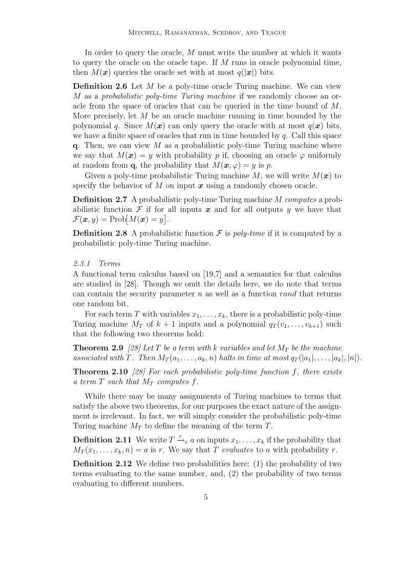
In order to query the oracle, M must write the number at which it wantsto query the oracle on the oracle tape. If M runs in oracle polynomial time,then M(x) queries the oracle set with at most q(|x|) bits.
Definition 2.6 Let M be a poly-time oracle Turing machine. We can viewM as a probabilistic poly-time Turing machine if we randomly choose an or-acle from the space of oracles that can be queried in the time bound of M .More precisely, let M be an oracle machine running in time bounded by thepolynomial q. Since M(x) can only query the oracle with at most q(x) bits,we have a finite space of oracles that run in time bounded by q. Call this spaceq. Then, we can view M as a probabilistic poly-time Turing machine wherewe say that M(x) = y with probability p if, choosing an oracle ϕ uniformlyat random from q, the probability that M(x, ϕ) = y is p.
Given a poly-time probabilistic Turing machine M , we will write M(x) tospecify the behavior of M on input x using a randomly chosen oracle.
Definition 2.7 A probabilistic poly-time Turing machine M computes a prob-abilistic function F if for all inputs x and for all outputs y we have thatF(x, y) = Prob
[M(x) = y
].
Definition 2.8 A probabilistic function F is poly-time if it is computed by aprobabilistic poly-time Turing machine.
2.3.1 Terms
A functional term calculus based on [19,7] and a semantics for that calculusare studied in [28]. Though we omit the details here, we do note that termscan contain the security parameter n as well as a function rand that returnsone random bit.
For each term T with variables x1, . . . , xk, there is a probabilistic poly-timeTuring machine MT of k + 1 inputs and a polynomial qT (v1, . . . , vk+1) suchthat the following two theorems hold:
Theorem 2.9 [28] Let T be a term with k variables and let MT be the machineassociated with T . Then MT (a1, . . . , ak, n) halts in time at most qT (|a1|, . . . , |ak|, |n|).
Theorem 2.10 [28] For each probabilistic poly-time function f , there existsa term T such that MT computes f .
While there may be many assignments of Turing machines to terms thatsatisfy the above two theorems, for our purposes the exact nature of the assign-ment is irrelevant. In fact, we will simply consider the probabilistic poly-timeTuring machine MT to define the meaning of the term T .
Definition 2.11 We write Tr−→e a on inputs x1, . . . , xk if the probability that
MT (x1, . . . , xk, n) = a is r. We say that T evaluates to a with probability r.
Definition 2.12 We define two probabilities here: (1) the probability of twoterms evaluating to the same number, and, (2) the probability of two termsevaluating to different numbers.
5

Mitchell, Ramanathan, Scedrov, and Teague
(i) Prob=
[T1, T2
]=
∑a s1s2,
where a ∈ N, T1s1−→e a, T2
s2−→e a, and
(ii) Prob6=[T1, T2
]=
∑〈a1,a2〉 s1s2,
where a1, a2 ∈ N, a1 6= a2, T1s1−→e a1, T2
s2−→e a2.
2.3.2 Processes
Definition 2.13 The syntax of processes is given by the following grammar:
P ::= 0 (termination)
νcp(|n|) .(P ) (private channel)
cp(|n|)(x).(P ) (input)
cp(|n|)〈T 〉 (output)
[T = T ].(P ) (match)
(P | P ) (parallel composition)
!γ(|n|).(P ) (γ(|n|)-fold replication)
Every input or output on a private channel must appear within the scope ofa ν-operator binding that channel. Otherwise the expression is consideredunevaluable.
Another word about channel names. The polynomial p(|n|) associated withthe channel c is a bandwidth parameter on c—for further details see section3.3. Also, as mentioned in section 2.3, no channel name is associated withmore than one polynomial.
For simplicity, after fixing n, when we evaluate a process P , we replace allsubexpressions of P of the form !γ(|n|).R with γ(|n|) copies of R in parallel.Furthermore, we define !γ(|n|).R to be left associative. Finally, we assume thatall channel names and variable names are α-renamed apart.
Finally, in what follows we will tend to omit parentheses if the parse treeof an expression is unambiguous.
Definition 2.14 We define an input expression as a process of the formcp(|n|)(x).P and an output expression is of the form cp(|n|)〈T 〉.
Definition 2.15 We call a process expression with no free variables a closedprocess expression.
Definition 2.16 Let P be a process expression and let T be a term. If Tis not in the scope of any input operator, we say that T is an exposed term.Similarly, let [T1 = T2].R be a subexpression of P . We will say that [T1 = T2].Ris an exposed match if it does not appear in the scope of any input operator.
6
Mitchell, Ramanathan, Scedrov, and Teague
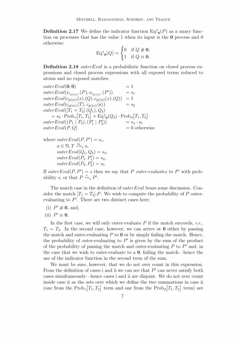
Definition 2.17 We define the indicator function Eq?0(P ) as a unary func-tion on processes that has the value 1 when its input is the 0 process and 0otherwise:
Eq?0(Q) =
{0 if Q 6≡ 0,
1 if Q ≡ 0.
Definition 2.18 outerEval is a probabilistic function on closed process ex-pressions and closed process expressions with all exposed terms reduced toatoms and no exposed matches:
outerEval(0,0) = 1outerEval(νcp(|n|) .(P ), νcp(|n|) .(P
′)) = s1
outerEval(cp(|n|)(x).(Q), cp(|n|)(x).(Q)) = 1outerEval(cp(|n|)〈T 〉, cp(|n|)〈a〉) = s2
outerEval([T1 = T2].(Q1), Q2)= s3 · Prob=
[T1, T2
]+ Eq?0(Q2) · Prob6=
[T1, T2
]outerEval((P1 | P2), (P
′1 | P ′
2)) = s4 · s5
outerEval(P, Q) = 0 otherwise.
where outerEval(P, P ′) = s1,
a ∈ N, Ts2−→e a,
outerEval(Q1, Q2) = s3,outerEval(P1, P
′1) = s4,
outerEval(P2, P′2) = s5
If outerEval(P, P ′) = s then we say that P outer-evaluates to P ′ with prob-ability s, or that P
s−→o P ′.
The match case in the definition of outerEval bears some discussion. Con-sider the match [T1 = T2].P . We wish to compute the probability of P outer-evaluating to P ′. There are two distinct cases here:
(i) P ′ 6≡ 0, and,
(ii) P ′ ≡ 0.
In the first case, we will only outer-evaluate P if the match succeeds, i.e.,T1 = T2. In the second case, however, we can arrive at 0 either by passingthe match and outer-evaluating P to 0 or by simply failing the match. Hence,the probability of outer-evaluating to P ′ is given by the sum of the productof the probability of passing the match and outer-evaluating P to P ′ and, inthe case that we wish to outer-evaluate to a 0, failing the match—hence theuse of the indicator function in the second term of the sum.
We must be sure, however, that we do not over count in this expression.From the definition of cases i and ii we can see that P ′ can never satisfy bothcases simultaneously—hence cases i and ii are disjoint. We do not over countinside case ii as the sets over which we define the two summations in case ii(one from the Prob=
[T1, T2
]term and one from the Prob 6=
[T1, T2
]term) are
7
Mitchell, Ramanathan, Scedrov, and Teague
disjoint.
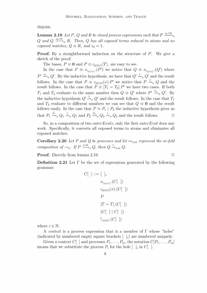
Lemma 2.19 Let P , Q and R be closed process expressions such that Ps1>0−−−→o
Q and Qs2>0−−−→o R. Then, Q has all exposed terms reduced to atoms and no
exposed matches, Q ≡ R, and s2 = 1.
Proof. By a straightforward induction on the structure of P . We give asketch of the proof.
The bases, P ≡ 0 and P ≡ cp(|n|)〈T 〉, are easy to see.
In the case that P ≡ νcp(|n|) .(P′) we notice that Q ≡ νcp(|n|) .(Q
′) where
P ′ s1−→o Q′. By the inductive hypothesis, we have that Q′ 1−→o Q′ and the result
follows. In the case that P ≡ cp(|n|)(x).P ′ we notice that P1−→o Q and the
result follows. In the case that P ≡ [T1 = T2].P′ we have two cases. If both
T1 and T2 evaluate to the same number then Q ≡ Q′ where P ′ t1−→o Q′. By
the inductive hypothesis Q′ 1−→o Q′ and the result follows. In the case that T1
and T2 evaluate to different numbers we can see that Q ≡ 0 and the resultfollows easily. In the case that P ≡ P1 | P2 the inductive hypothesis gives us
that P1
s′1−→o Q11−→o Q1 and P2
s′2−→o Q21−→o Q2 and the result follows. 2
So, in a composition of two outerEvals, only the first outerEval does anywork. Specifically, it converts all exposed terms to atoms and eliminates allexposed matches.
Corollary 2.20 Let P and Q be processes and let −→o,m represent the m-fold
composition of −→o. If Ps>0−−→o Q, then Q
1−→o,m Q.
Proof. Directly from lemma 2.19. 2
Definition 2.21 Let Γ be the set of expressions generated by the followinggrammar:
C[ ] ::= [ ]i
νcp(|n|) .(C[ ])
cp(|n|)(x).(C[ ])
P
[T = T ].(C[ ])
(C[ ] | C[ ])
!γ(|n|).(C[ ])
where i ∈ N.
A context is a process expression that is a member of Γ whose “holes”(indicated by numbered empty square brackets [ ]i) are numbered uniquely.
Given a context C[ ] and processes P1, . . . , Pm, the notation C[P1, . . . , Pm]means that we substitute the process Pi for the hole [ ]i in C[ ].
8
Mitchell, Ramanathan, Scedrov, and Teague
Finally, we will indicate the number of holes is a context by placing an(often un-numbered) empty square bracket for each hole in the context. Forexample, C[ ] will be a one-hole context while D[ ][ ][ ] has three holes.
Definition 2.22 We will say that B is a sub-process of A if there exists acontext C[ ] such that C[B] ≡ A. If C[ ] 6≡ [ ] we will say that B is a strictsub-process of A.
Definition 2.23 Let P and Q be process expressions and cp(|n|) be a channel.We say that P is bound by cp(|n|) in Q if cp(|n|)(x).D[P ] is a sub-process of Qfor some variable x and some context expression D[ ].
Definition 2.24 Let C[ ] be a context and P a process. Then, C[ ] isminimal for P if every free variable of P is bound in C[P ] and each channelto which P is bound in C[P ] binds a free variable of P .
Definition 2.25 The set of schedulable processes S(P ) of an outer-evaluatedprocess P is defined inductively as:
S(0) = ∅
S(νcp(|n|) .(Q)) = S(Q)
S(cp(|n|)(x).(Q)) = {cp(|n|)(x).(Q)}
S(cp(|n|)〈T 〉) = {cp(|n|)〈T 〉}
S((Q1 | Q2)) = S(Q1) ∪ S(Q2)
Note that every process in S(P ) is either waiting for input or ready tooutput.
Definition 2.26 The set of communication triples C(P ) is defined as:
{〈P1, P2, QP1,P2 [ ]〉|P1 ≡ cp(|n|)〈a〉, P2 ≡ cp(|n|)(x).R,
Pi ∈ S(P ),
P ≡ QP1,P2 [P1, P2]}
Given a process P and a context QP1,P2 [ ], P1 and P2 are uniquely deter-mined.
Example 2.27 Consider the process expression:
P ≡ cp(|n|)〈0〉 | cp(|n|)〈0〉 | cp(|n|)(x).dq(|n|)〈1〉
The process expression cp(|n|)(x).dq(|n|)〈1〉 could receive its input from eitherone of the two output expressions. While both communications look the same,their outputs come from distinct locations in P . We distinguish between thetwo communications by associating the context [ ]1 | cp(|n|)〈0〉 | [ ]2 with the
9
Mitchell, Ramanathan, Scedrov, and Teague
first communication (the one where the output ‘came’ from the first processin the parallel composition) and associating the context cp(|n|)〈0〉 | [ ]1 | [ ]2with the second communication (the pair where the output ‘came’ from thesecond process in the parallel composition). So, C(P ) is the set:{
〈cp(|n|)〈0〉, cp(|n|)(x).dq(|n|)〈1〉, [ ]1 | cp(|n|)〈0〉 | [ ]2〉 ,
〈cp(|n|)〈0〉, cp(|n|)(x).dq(|n|)〈1〉, cp(|n|)〈0〉 | [ ]1 | [ ]2〉}
Definition 2.28 The set of eligible processes E(P ) is defined as:
E(P ) =
C(P )iff every channel inC(P ) is public,
C(P )|private channels otherwise.
Note that restricting E(P ) to just private channels anytime C(P ) containsa private channel ensures that all private communications occurs prior topublic communication. This allows us to “hide” private communications froma prying observer by making private communications privileged.
3 Evaluation
3.1 Scheduler Reduction
Definition 3.1 We write [a/x] P to mean “substitute a for all free occur-rences of x in P .” We will define the substitution operation as follows:
[a/x]0 = 0
[a/x] νcp(|n|) .(Q) = νcp(|n|) .([a/x] Q)
[a/x] cp(|n|)(y).(Q) = cp(|n|)(y).([a/x] Q)
[a/x] cp(|n|)(x).(Q) = cp(|n|)(x).(Q)
[a/x] cp(|n|)〈T 〉 = cp(|n|)〈(λx.T ) a〉
[a/x] [T1 = T2].(Q) = [(λx.T1) a = (λx.T2) a].([a/x] Q)
[a/x] (P1 | P2) = ([a/x] P1 | [a/x] P2)
[a/x]!γ(|n|).(Q) = !γ(|n|).([a/x] Q)
We can generalize the substitution operation to contexts, i.e., to substitutinga for all free occurrences of x in C[ ].
Definition 3.2 We define a scheduler S to be a probabilistic function fromsets of communication triples to communication triples such that for every setof communication triples E, if S(E, e) > 0 then e ∈ E. If S(E, e) = r we will
10
Mitchell, Ramanathan, Scedrov, and Teague
say that the scheduler S picks the communication triple e from the set E withprobability r.
Definition 3.3 Let a be a natural number, n the value of the security param-eter, and S a scheduler. We will say that P reduces to P ′ in one communicationstep with respect to S with probability r if and only if:
∃e ≡ 〈P1, P2, QP1,P2 [ ]〉 ∈ E(P ) : S(E(P ), e) = r,
P1 ≡ cp(|n|)〈a〉,
P2 ≡ cp(|n|)(x).P ′2,
P ′ ≡ QP1,P2 [0, [a′/x]P ′2] ,
a′ = a mod 2p(|n|) − 1.
We write this as Pr−→S P ′.
We reduce a modulo 2p(|n|) − 1 in order to ensure that at most only thep(|n|) least significant bits of a are transmitted.
By stipulating that at most p(|n|) bits of a message can be transmitted weensure that we cannot create exponential-time processes out of polynomial-time process expressions—something that we can do if we allowed arbitrarylength messages to be transmitted. Consider the process expression:
P ≡ !γ(|n|).cp(|n|)(x).cp(|n|)〈x2〉 | cp(|n|)〈2〉
Let the polynomial γ(|x|) return x always. While more complex polynomialswill make the results more dramatic, this choice of γ simplifies matters. It isclear that P will square its input (here initialized to 2) n times. We will callthe output of this process Pn.
The table below shows outputs for several different values of n:
n Pn |Pn|
1 4 = 22 2 = 21
2 16 = 24 4 = 22
3 256 = 28 8 = 23
4 65, 536 = 216 16 = 24
5 4, 294, 967, 296 = 232 32 = 25
......
...
Clearly, P outputs values of length exponential in n. Now if the output of P isused as the input to some poly-time process expression Q, then we will obtainan exponential-time process since Q must run on exponentially long values.
11
Mitchell, Ramanathan, Scedrov, and Teague
However, if we truncate the messages transmitted then no message can everget too long, i.e., exponentially long.
3.2 Evaluation
3.2.1 Macro-Step Reduction
Intuitively, we define the macro-step reduction of P to P ′ based on the follow-ing three stage procedure:
(i) We outer-evaluate P , yielding R.
(ii) The scheduler picks a process triple E from E(R) and performs the se-lected communication. This results in the process expression R′.
(iii) Finally, we outer-evaluate R′, yielding P ′.
Thus, macro-step reduction is merely shorthand for a procedure whereby weselect a communication to perform and evaluate the result until it becomes nec-essary for the next communication to be selected. The first outer-evaluationsimply ensures that the process expression on which we perform the commu-nication step satisfies the condition on S(P ) specified in defn. 2.25. Barringthe first outer-evaluation, then, the evaluation of process expressions becomesan alternating series of process evaluations (the outer-evaluations) and com-munication steps. We will define macro-step reduction so that it is just acommunication step followed by a process evaluation—with a preceding pro-cess evaluation for the reason mentioned above.
Definition 3.4 More precisely, macro-step reduction with respect to schedulerS is the probabilistic function defined by the composition:
−→o ◦ (−→S ◦ −→o) (3a)
The probability r of the macro-step reduction of P to P ′ is obtained directlyfrom definition 2.2:
r =∑
Q,Q′|Pa−→oQ
b−→SQ′ c−→oP ′
abc (3b)
We will write the macro-step reduction of P to P ′ with respect to the schedulerS with probability r as P
r−→1,S P ′.
3.2.2 m-Step Reduction
Definition 3.5 Let P and P ′ be two process expressions. Define the setPathsP,P ′ as:
{{Q1, . . . , Qm−1}|Pp1−→1,S Q1
p2−→1,S · · ·pm−1−−−→1,S Qm−1
pm−→1,S P ′}
We call PathsP,P ′ the set of paths from P to P ′.
12
Mitchell, Ramanathan, Scedrov, and Teague
Definition 3.6 The probability that P reduces to P ′ in m steps with respectto the scheduler S is given by: ∑
{Q1,··· ,Qm−1}∈PathsP,P ′
Pp1−→1,SQ1
p2−→1,S ···pm−1−−−→1,SQm−1
pm−→1,SP ′
p1p2 · · · pm
We write the m-step reduction of P to P ′ with probability r as Pr−→m,S P ′.
3.2.3 Evaluation
Definition 3.7 We say that P evaluates to Q with respect to the scheduler Sif, using the scheduler S, P reduces to Q via some number of macro-steps. Wewrite the evaluation of P to P ′ with respect to the scheduler S as P ↪→S P ′.
4 Polynomial-Time Bound on Evaluation
We are interested in the worst-case time of evaluation. Since the probability ofa particular reduction has no bearing on the worst-case time of evaluation, weneed not consider the probabilities of the various reductions in our analysis.
Our bound on evaluation will be derived as a certain combination of threebounds: a bound on the length of any evaluation sequence, a bound on anyouter-evaluation step, and a bound on any communication step.
4.1 A Bound on the Length of any Evaluation Sequence
Definition 4.1 Let P be a process expression. We define inputs(P ), thenumber of inputs in P , inductively as follows:
inputs(0) = 0
inputs(νcp(|n|) .(Q)) = inputs(Q)
inputs(cp(|n|)(x).(Q)) = 1 + inputs(Q)
inputs(cp(|n|)〈T 〉) = 0
inputs([T1 = T2].(Q)) = inputs(Q)
inputs((Q1 | Q2)) = inputs(Q1) + inputs(Q2)
inputs(!γ(|n|).(Q)) = γ(|n|) · inputs(Q)
It is clear from the definition that inputs(P ) is a polynomial in |n| that ispositive for all input values.
Definition 4.2 Let P be a process expression. We define outputs(P ), the
13
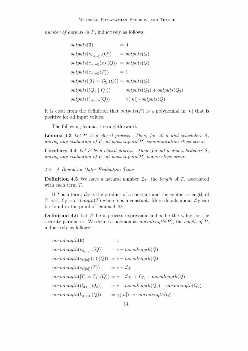
Mitchell, Ramanathan, Scedrov, and Teague
number of outputs in P , inductively as follows:
outputs(0) = 0
outputs(νcp(|n|) .(Q)) = outputs(Q)
outputs(cp(|n|)(x).(Q)) = outputs(Q)
outputs(cp(|n|)〈T 〉) = 1
outputs([T1 = T2].(Q)) = outputs(Q)
outputs((Q1 | Q2)) = outputs(Q1) + outputs(Q2)
outputs(!γ(|n|).(Q)) = γ(|n|) · outputs(Q)
It is clear from the definition that outputs(P ) is a polynomial in |n| that ispositive for all input values.
The following lemma is straightforward.
Lemma 4.3 Let P be a closed process. Then, for all n and schedulers S,during any evaluation of P , at most inputs(P ) communication steps occur.
Corollary 4.4 Let P be a closed process. Then, for all n and schedulers S,during any evaluation of P , at most inputs(P ) macro-steps occur.
4.2 A Bound on Outer-Evaluation Time
Definition 4.5 We have a natural number LT , the length of T , associatedwith each term T .
If T is a term, LT is the product of a constant and the syntactic length ofT , i.e., LT = c · length(T ) where c is a constant. More details about LT canbe found in the proof of lemma 4.10.
Definition 4.6 Let P be a process expression and n be the value for thesecurity parameter. We define a polynomial normlength(P ), the length of P ,inductively as follows:
normlength(0) = 1
normlength(νcp(|n|) .(Q)) = c + normlength(Q)
normlength(cp(|n|)(x).(Q)) = c + normlength(Q)
normlength(cp(|n|)〈T 〉) = c + LT
normlength([T1 = T2].(Q)) = c + LT1 + LT2 + normlength(Q)
normlength((Q1 | Q2)) = c + normlength(Q1) + normlength(Q2)
normlength(!γ(|n|).(Q)) = γ(|n|) · c · normlength(Q)
14
Mitchell, Ramanathan, Scedrov, and Teague
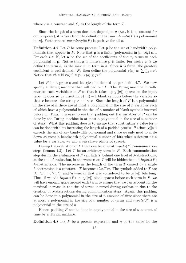
where c is a constant and LT is the length of the term T .
Since the length of a term does not depend on n (i.e., it is a constant forour purposes), it is clear from the definition that normlength(P ) is polynomialin |n|. Furthermore, normlength(P ) is positive for all n.
Definition 4.7 Let P be some process. Let p be the set of bandwidth poly-nomials that appear in P . Note that p is a finite (polynomial in |n| big) set.For each i ∈ N, let a be the set of the coefficients of the xi terms in eachpolynomial in p. Notice that a is finite since p is finite. For each i ∈ N wedefine the term ai as the maximum term in a. Since a is finite, the greatestcoefficient is well-defined. We then define the polynomial χ(x) as
∑∞i=0 aix
i.Notice that ∀b ∈ N.∀p(x) ∈ p : χ(b) ≥ p(b).
Let P be a process and let χ(x) be defined as per defn. 4.7. We nowspecify a Turing machine that will pad out P . The Turing machine initiallyrewrites each variable x in P so that it takes up χ(|n|) spaces on the inputtape. It does so by inserting χ(|n|) − 1 blank symbols before the variable sothat x becomes the string M · · · M x. Since the length of P is a polynomialin the size of n there are at most a polynomial in the size of n variables eachof which have a polynomial in the size of n number of blank symbols insertedbefore it. Thus, it is easy to see that padding out the variables of P can bedone by the Turing machine in at most a polynomial in the size of n numberof steps. What this padding does is to ensure that substituting a value for xcan be done without increasing the length of a padded process P (since χ(|n|)exceeds the size of any bandwidth polynomial and since we only need to writedown at most a bandwidth polynomial number of bits when substituting avalue for a variable, we will always have plenty of space).
During the evaluation of P there can be at most inputs(P ) communicationsteps (lemma 4.3). Let T be an arbitrary term in P . Each communicationstep during the evaluation of P can hide T behind one level of λ-abstractions;at the end of evaluation, in the worst case, T will be hidden behind inputs(P )λ-abstractions. The increase in the length of the term T caused by a singleλ-abstraction is a constant—T becomes (λx.T )a. The symbols added to T are‘λ’, ‘x’, ‘.’, ‘(’, ‘)’ and ‘a’—recall that a is considered to be χ(|n|) bits long.Thus, if we add inputs(P ) · c · χ(|n|) blank spaces before each term in P , wewill have enough space around each term to ensure that we can account for themaximal increase in the size of terms incurred during evaluation due to thecreation of λ-abstractions during communication steps. Again, this paddingcan be done in a polynomial in the size of n amount of time since there areat most a polynomial in the size of n number of terms and inputs(P ) is apolynomial in the size of n.
Hence, padding P can be done in a polynomial in the size of n amount oftime by a Turing machine.
Definition 4.8 Let P be a process expression and n be the value for the
15
Mitchell, Ramanathan, Scedrov, and Teague
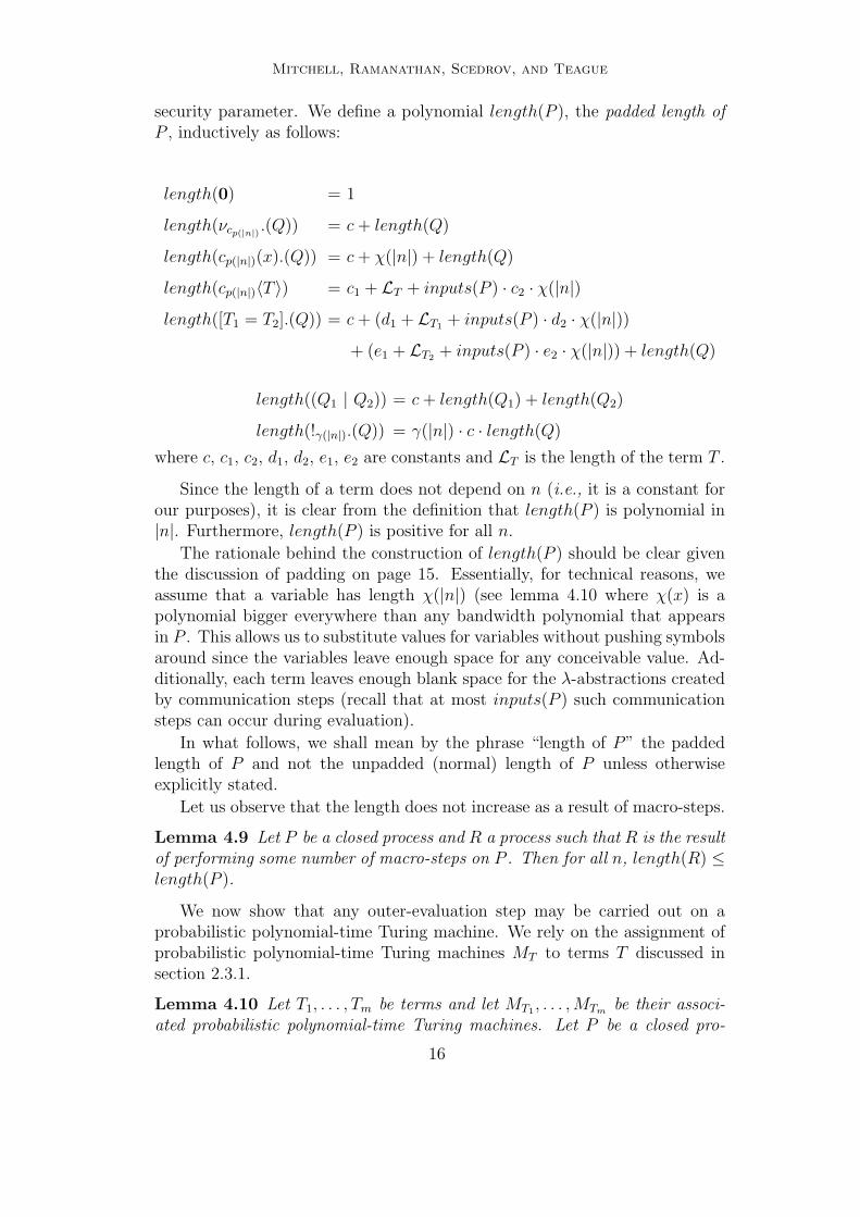
security parameter. We define a polynomial length(P ), the padded length ofP , inductively as follows:
length(0) = 1
length(νcp(|n|) .(Q)) = c + length(Q)
length(cp(|n|)(x).(Q)) = c + χ(|n|) + length(Q)
length(cp(|n|)〈T 〉) = c1 + LT + inputs(P ) · c2 · χ(|n|)
length([T1 = T2].(Q)) = c + (d1 + LT1 + inputs(P ) · d2 · χ(|n|))
+ (e1 + LT2 + inputs(P ) · e2 · χ(|n|)) + length(Q)
length((Q1 | Q2)) = c + length(Q1) + length(Q2)
length(!γ(|n|).(Q)) = γ(|n|) · c · length(Q)
where c, c1, c2, d1, d2, e1, e2 are constants and LT is the length of the term T .
Since the length of a term does not depend on n (i.e., it is a constant forour purposes), it is clear from the definition that length(P ) is polynomial in|n|. Furthermore, length(P ) is positive for all n.
The rationale behind the construction of length(P ) should be clear giventhe discussion of padding on page 15. Essentially, for technical reasons, weassume that a variable has length χ(|n|) (see lemma 4.10 where χ(x) is apolynomial bigger everywhere than any bandwidth polynomial that appearsin P . This allows us to substitute values for variables without pushing symbolsaround since the variables leave enough space for any conceivable value. Ad-ditionally, each term leaves enough blank space for the λ-abstractions createdby communication steps (recall that at most inputs(P ) such communicationsteps can occur during evaluation).
In what follows, we shall mean by the phrase “length of P” the paddedlength of P and not the unpadded (normal) length of P unless otherwiseexplicitly stated.
Let us observe that the length does not increase as a result of macro-steps.
Lemma 4.9 Let P be a closed process and R a process such that R is the resultof performing some number of macro-steps on P . Then for all n, length(R) ≤length(P ).
We now show that any outer-evaluation step may be carried out on aprobabilistic polynomial-time Turing machine. We rely on the assignment ofprobabilistic polynomial-time Turing machines MT to terms T discussed insection 2.3.1.
Lemma 4.10 Let T1, . . . , Tm be terms and let MT1 , . . . ,MTm be their associ-ated probabilistic polynomial-time Turing machines. Let P be a closed pro-
16
Mitchell, Ramanathan, Scedrov, and Teague
cess containing terms (λx1 · · ·λxr.Tj) a1 · · · ar, where 1 ≤ j ≤ m. FromMT1 , . . . ,MTm one can construct a probabilistic Turing machine that outer-evaluates P in time polynomial in |n|.
Proof. Let us make the following two assumptions. First, we assume thatvariables have length χ(|n|). This ensures that when we substitute a value(recall that the length of values are limited by the appropriate bandwidthpolynomials due to the truncation in the communication step) for a variable,it is easy to replace the variable with the value, i.e., we do not need to “push”forward the symbols following the variable in order to make room for the valuewe want to write down.
Second, we assume that when we evaluate a term, we only write downthe χ(|n|) least significant bits of the resultant value. In principle we allowarbitrarily large values to be written down—it is only during communicationthat these values are truncated. However, this means that as terms evaluatethe process expression we are working on might arbitrarily increase in size.Since the only time a value created by a term evaluation is used occurs whenwe communicate the value, truncating the value at creation does not changeanything. It is true that values generated by term evaluations are used in thematch—however we do not write down these values; we simply write downeither 0 or the result of outer-evaluating the process expression bound to thematch.
The result of these two assumptions is that each outer-evaluation eitherdoes not change the length of the process or decreases the length of the process(by replacing inputs and outputs with 0s and evaluating matches).
If we pad P prior to outer-evaluating it we can guarantee these assump-tions. Furthermore the padding can be done, as we have seen, in a polynomialin size n amount of time.
We will now construct the desired probabilistic Turing machine, pTM. Es-sentially, the pTM must evaluate each exposed term and each exposed matchin P (it is easy to determine if a term or match is exposed—every time an in-put operator, say cp(|n|)(x).P , is encountered, we consider every subexpressionof P as being not exposed). Since we know that P will only contain terms thatare substitution instances of terms from the set {T1, . . . , Tm}, we can associateeach term Ui from P with an algorithm MTi′
where Ti′ is the term of whichUi is a substitution instance. By theorem 2.9 we have that MTi′
computes,in polynomial time, the value to which Ti′ evaluates on some input. Since Ui
is a substitution instance of Ti′ we have that Ui ≡ (λx1 · · ·λxr.Ti′) a1 · · · ar.Hence, we can compute the value of Ui by evaluating MTi′
at a1, . . . , ar and n.
So we define our pTM so that when it encounters a substitution instanceof one of those m terms, it invokes the appropriate algorithm (in the casethat it encountered Ui ≡ (λx1 · · ·λxi.Ti′) a1 . . . ai, it invokes MTi′
at a1, . . . , a1
and n). Recall that each communication step creates λ-substitution instancesof terms, i.e., the substitution of values into terms is delayed until term-
17
Mitchell, Ramanathan, Scedrov, and Teague
evaluation time. So, our pTM evaluates each exposed term it encounters byevaluating the associated algorithm at the values specified by the substitutioninstance. Evaluating a match simply involves evaluating the two terms andwriting either the 0 or outer-evaluating the bound process.
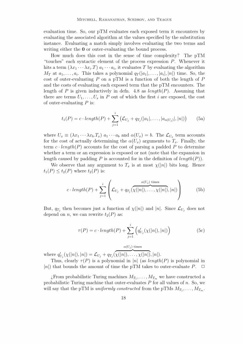
How much does this cost in the sense of time complexity? The pTM“touches” each syntactic element of the process expression P . Whenever ithits a term (λx1 · · ·λxi.T ) a1 · · · ai, it evaluates T by evaluating the algorithmMT at a1, . . . , ai. This takes a polynomial qT (|a1|, . . . , |ai|, |n|) time. So, thecost of outer-evaluating P on a pTM is a function of both the length of Pand the costs of evaluating each exposed term that the pTM encounters. Thelength of P is given inductively in defn. 4.8 as length(P ). Assuming thatthere are terms U1, . . . , Us in P out of which the first i are exposed, the costof outer-evaluating P is:
t1(P ) = c · length(P ) +i∑
j=1
(LUj
+ qTj(|a1|, . . . , |aα(Uj)|, |n|)
)(5a)
where Ux ≡ (λx1 · · ·λxb.Tx) a1 · · · ab and α(Ux) = b. The LUx term accountsfor the cost of actually determining the α(Ux) arguments to Tx. Finally, theterm c · length(P ) accounts for the cost of parsing a padded P to determinewhether a term or an expression is exposed or not (note that the expansion inlength caused by padding P is accounted for in the definition of length(P )).
We observe that any argument to Tx is at most χ(|n|) bits long. Hencet1(P ) ≤ t2(P ) where t2(P ) is:
c · length(P ) +i∑
j=1
LUj+ qTj
(
α(Uj) times︷ ︸︸ ︷χ(|n|), . . . , χ(|n|), |n|)
(5b)
But, qTjthen becomes just a function of χ(|n|) and |n|. Since LUj
does notdepend on n, we can rewrite t2(P ) as:
τ(P ) = c · length(P ) +i∑
j=1
(q′Uj
(χ(|n|), |n|))
(5c)
where q′Uj(χ(|n|), |n|) = LUj
+ qTj(
α(Uj) times︷ ︸︸ ︷χ(|n|), . . . , χ(|n|), |n|).
Thus, clearly τ(P ) is a polynomial in |n| (as length(P ) is polynomial in|n|) that bounds the amount of time the pTM takes to outer-evaluate P . 2
¿From probabilistic Turing machines MT1 , . . . ,MTm we have constructed aprobabilistic Turing machine that outer-evaluates P for all values of n. So, wewill say that the pTM is uniformly constructed from the pTMs MT1 , . . . ,MTm .
18

Mitchell, Ramanathan, Scedrov, and Teague
Definition 4.11 We define κ(P ), the cost of outer-evaluating a closed processexpression P , as:
κ(P ) = c · length(P ) +s∑
j=1
(q′Tj
(χ(|n|), |n|))
where the process P has the terms T1, . . . , Ts and q′Tjis defined as for equation
(5c) and c is a constant that accounts for the cost of parsing a padded P todetermine exposed expressions and terms.
Whereas τ(P ) is the time needed to outer-evaluate just the exposed termsand matches in P , κ(P ) is the cost of outer-evaluating every term and matchin P . The following lemma is immediate.
Lemma 4.12 Let P be a closed process. Then, τ(P ) ≤ κ(P ).
It may also be shown that macro-steps do not increase the cost of outer-evaluation.
Lemma 4.13 Let P be a closed process expression and S a scheduler. Let Rbe a process such that R is obtained by performing a finite number of macro-steps on P . Then for all n and k, κ(R) ≤ κ(P ).
Thus we also obtain
Lemma 4.14 Let P be a closed process. Let R be a process such that Pevaluates to R in at most m macro-steps. Then τ(R) ≤ κ(P ).
4.3 A Bound on the Communication Step
Lemma 4.15 Let P be a closed process and π a communication triple. Thenthere exists a pTM such that for all P , π, n and k, the pTM performs thecommunication step indicated by π on P in time polynomial in |n|.
Proof. We begin by padding P . This allows us to assume, as we did in theproof of lemma 4.10, that variables are χ(|n|) bits long. This means that wecan easily substitute values for variables by simply overwriting the variable.
In order to perform the communication step, we make one pass to removethe input and output specified in π. Specifically, we rewrite the subexpressioncp(|n|)(x).Q specified as the input in π with MMMMMQ (where M is a specialcharacter that the pTM ignores—this allows us to delete subexpressions ofP without having to push symbols around) and we rewrite the subexpressioncp(|n|)〈a〉 specified as the output in π with MMM0. So, the pTM performs apass, prior to performing the substitution indicated by the communicationstep, to eliminate the input and output process expressions.
We then make another pass over the process replacing all instances of xwith a. Since we assume that all channels are α-renamed apart and that botha and x are at most χ(|n|) bits long, we can do this substitution without any
19
Mitchell, Ramanathan, Scedrov, and Teague
real effort except when we create a λ-substitution instance out of a term T .When this happens, we need to insert symbols. However, each communicationstep adds one level of λ-abstraction; so, when we write the process down weleave sufficient room around each term T , i.e., we add some fixed amount ofblank space after each term. Since the notation for a single λ-abstraction isconstant sized and the value to apply to that λ-abstraction is at most χ(|n|)bits long, a fixed amount of space per term will suffice. We added this extraspace to each term during the initial pass that padded out P . Essentially, weare adding a polynomial in |n| amount of padding to the process—the lengthof the expression is a polynomial in |n| and an upper-bound on the number ofterms in the process.
Then, we can easily perform the needed rewriting necessitated by the com-munication step without moving symbols around. Thus, a single pass over theprocess should suffice to perform the communication step.
So, the time needed to perform the communication step is just σ(P ) =c0 · length(P ) where c0 is a constant that accounts for the multiple passes (oneto eliminate the input and output expressions and another to perform the sub-stitutions indicated by the communication step) and length(P ) accounts forthe increased length caused by padding out P . Clearly, σ(P ) is a polynomialin |n| since length(P ) is such a polynomial. 2
Definition 4.16 Let P be a process expression. We notice that if thereare inputs(P ) inputs and outputs(P ) outputs in P , then there are at mostinputs(P ) · outputs(P ) communication steps possible. Let ci be the constantfactor that accounts for the multiples passes incurred during the evaluation ofthe ith communication step (meaning, the ith communication out of the setof inputs(P ) · outputs(P ) communication steps; not the communication takenat the ith evaluation step).
We define ϕ(P ), the cost of performing a substitution given by a commu-nication triple π on the closed process expression P , as:
ϕ(P ) = c0 · length(P ) + c1 · length(P ) + · · ·+ ck · length(P )
where k = inputs(P ) · outputs(P ).
σ(P ) is the time needed to perform the substitution specified by π. How-ever, ϕ(P ) is meant to bound the cost of any substitution that might possiblyoccur in the course of evaluating P . A process has inputs(P ) inputs andoutputs(P ) outputs. Since an arbitrary substitution consists of one input ex-pression and one output expression, there are at most inputs(P ) · outputs(P )possible communications that can occur. At any communication step (bylemma 4.4, there are at most inputs(P ) such steps), only one potential com-munication occurs. Hence ϕ is an upper bound on the time needed to performany communication that might occur in the evaluation of P .
It is clear that
20
Mitchell, Ramanathan, Scedrov, and Teague
Lemma 4.17 Let P be a closed process. Then, σ(P ) ≤ ϕ(P ).
It follows from lemmas 4.9 and 4.17 that
Lemma 4.18 Let P be a closed process expression and S a scheduler. Let Rbe a process such that R is obtained by a finite number of macro-steps fromP . Then for all n, σ(R) ≤ ϕ(P ).
4.4 A Bound on Evaluation Time
We now use the bounds obtained in the previous three subsections to obtaina polynomial bound on total evaluation time.
Definition 4.19 Let P be a process expression. We define an evaluationcontext for P as a context C[ ] of the form:
c1p1(|n|)(x1) . . . cipi(|n|)(xi).[ ] | c1p1(|n|)〈a1〉 | · · · | ctpt(|n|)〈at〉
where t = i + inputs(P ), there are no free variables in C[P ], aj ∈ N, and eachx1, · · · , xi either appears free in P or does not appear at all in P .
We will sometimes specify that the evaluation context C[ ] is an (i, t)-evaluation context, meaning that it has i inputs and t outputs.
If P is a process and C[ ] is an evaluation context for P , then C[P ] is aclosed process.
Definition 4.20 Let P ≡ P1 | · · · | Pm be a process such that P is theresult of outer-evaluating some process expression Q. If, for each Pi such thatPi ≡ cp(|n|)(x).P ′
i there does not exist a Pj with j 6= i such that Pj ≡ cp(|n|)〈a〉,we say that P is a normal form.
It should be clear from defn. 4.20 that if a process P is a normal form,then P cannot be further evaluated as E(P ) = ∅.
Theorem 4.21 Let P be a process expression. Then, there exists a polyno-mial q(x) with all positive coefficients such that for all n, all poly-time sched-ulers S and minimal evaluation contexts C[ ] for P , the process C[P ] evaluatesto a normal form on a probabilistic Turing machine in time at most q(|n|).
The idea behind this theorem is that given a process P (that is possiblynot closed) and an evaluation context C[ ] that closes P and provides P withall the necessary inputs, C[P ] evaluates, on a probabilistic Turing machine,to a normal form in at most polynomial time.
Proof. By lemma 4.3, we have that at most inputs(C[P ]) (recall that this isa polynomial in |n|—see defn. 4.1) communication steps (and hence macro-steps) occur during the evaluation. Thus, all we need to do is determine thetime it takes to perform a macro-step.
We note that the second outer-evaluation of a macro-step composes withthe first outer-evaluation of the next macro-step. Since outer-evaluation is
21

Mitchell, Ramanathan, Scedrov, and Teague
idempotent (lemma 2.19), neither the probability distribution nor the resul-tant process changes as a consequence of the double outer-evaluation. All thathappens is that we take a little extra time.
The time to outer-evaluate any process that can be obtained by a reductionfrom C[P ] on a Turing machine is given by lemma 4.14 as a polynomial in|n|—call this qo(|n|). Recall that outer-evaluation is performed by making apass over the process expression and replacing each exposed term that hasno free variables with a number (truncated so that its size doesn’t exceed theband-width of the channel). In the case of matches, we do not write downthe value of the two terms being compared. Instead we outer-evaluate thebound process or write down 0. Since the length of C[P ] is polynomial in |n|outer-evaluation takes time polynomial in |n|.
The time to perform any communication step that might arise in the eval-uation of C[P ] is given by lemma 4.18 as a polynomial, qc, in |n|. Recall thata communication step that substitutes a for x is performed by making a passover the process expression and replacing each instance of the variable x witha. Since the length of C[P ] is polynomial in |n| communication takes timepolynomial in |n|.
However, there is an additional cost incurred in actually selecting the com-munication step. It requires a single pass over the process expression to buildS(C[P ]) and then time proportional in |S(C[P ])| to build E(C[P ]). But thereare at most inputs(C[P ]) input expressions and outputs(C[P ]) output expres-sions in C[P ]. Consequently |S(C[P ])| is at most inputs(C[P ])·outputs(C[P ])which is a polynomial in |n|. Consequently, generating E(C[P ]) from C[P ]takes polynomial in |n| time.
Furthermore, the scheduler is defined to be poly-time, i.e., given the eli-gible process set E(C[P ]), the scheduler takes a polynomial in |E(C[P ])| =|S(C[P ])|2 amount of time to choose a communication step. But this is just apolynomial in |n|. Hence, in order to generate E(C[P ]) and make a choice werequire a polynomial, qd, in |n| amount of time. Since macro-steps do not in-crease the length of a process expression, qd is an upper-bound on the amountof time required to schedule a communication when evaluating R where R isa process expression obtained from C[P ] via some number of macro-steps.
Hence the time needed for evaluation q is given by:
inputs(C[P ]) ·(qo(|n|) + qd(|n|) + qc(|n|) + qo(|n|)
)(6)
which is just a polynomial in |n|. 2
5 Equivalence
Definition 5.1 We define an observation to be a test on a particular publicchannel for a particular natural number. More precisely, we will define Obsto be the set of all possible observations, i.e., the set of pairs 〈i, cp(|n|)〉 where
22
Mitchell, Ramanathan, Scedrov, and Teague
i ∈ [0..2p(|n|)− 1] is a natural number and cp(|n|) is a public channel. If, duringan evaluation of process expression P , the scheduler selects the communicationtriple 〈cp(|n|)〈i〉, cp(|n|)(x).P ′, Qcp(|n|)〈i〉,cp(|n|)(x).P ′〉 we will say that the observable〈i, cp(|n|)〉 ∈ Obs was observed and write P ; 〈i, cp(|n|)〉.
Definition 5.2 Let ∆ be the set of expressions generated by the followingsub-grammar of the one which produces contexts (see defn. 2.21):
C[ ] ::= [ ]i
cp(|n|)(x).(C[ ])
P
[T = T ].(C[ ])
(C[ ] | C[ ])
!γ(|n|).(C[ ])
where i ∈ N.
An adversarial context is a process expression that is a member of ∆—∆is just the subset of the set of contexts (Γ) where a hole doesn’t appear in thescope of a ν-operator. As for a standard context, the “holes” are numbereduniquely.
Definition 5.3 A process P may contain the security parameter n (section2.3). We will write Pm to signify that the parameter n is assigned the naturalnumber m. A process family P is the set 〈Pi| i ∈ N〉. Since contexts maycontain the process parameter n, we can define the context family C[ ] andthe adversarial context family C[ ] analogously.
We evaluate a process family by picking a value for n and then evaluatingthe indicated member of the process family. In this manner we can extendall the concepts regarding process expressions and contexts to process andcontext families.
Definition 5.4 We define P to be the set of all process families, C to bethe set of all context families and A to be the set of all adversarial contextfamilies.
5.1 Observational Equivalence
Definition 5.5 Let P be a process family. We will say that the channel namecq(|n|) appears in P just when there are inputs and outputs on cq(|n|) that aresubexpressions of P .
Definition 5.6 Let P and Q be two process families. Let q be the set ofpolynomials q(x) such that ∀y : q(y) > 0. We will say that P and Q are
23

Mitchell, Ramanathan, Scedrov, and Teague
observationally equivalent if:
∀q(x) ∈ q.∀C[ ] ∈ A.∀o ∈ Obs.∃no.∀n > no :∣∣ Prob[Cn[Pn] ; o
]− Prob
[Cn[Qn] ; o
]∣∣ ≤ 1
q(n)
If this is so, we will write that P ∼= Q.
It is our goal to define adversaries to a protocol as adversarial contexts.Then, we will be able to prove security properties by stating observationalequivalences.
The idea here is that if two process families are the same, then no adver-sarial context (i.e., attacker) can distinguish between the two with significantprobability once the security parameter gets large enough—the probability ofone process family producing an observable is indistinguishable (to within anarbitrary polynomial factor) from the probability of the other process familyproducing that same observable.
However, if we forced observational equivalence to hold under all con-texts, then we are essentially saying that adversaries can attack a protocolby changing the way a protocol executes (by specifying the scope of a pri-vate channel and, thereby, being able to read values transmitted on privatechannels). However, such attacks do not seem appropriate given our model ofadversary capabilities. Hence, we discount such contexts from our definitionof observational equivalence.
We can only guarantee such a property in the case that n is large enoughas most any security system can be defeated by brute-force searches if thesearch-space is small enough. So, even though a context (i.e., a brute forcesearch over, say, keys) may distinguish two process families (that is break oneprotocol and not the other), once we up the security parameter sufficiently,that context will get defeated.
Proposition 5.7 ∼= is an equivalence relation.
Because the definition of observational equivalence involves all adversarialcontexts (definition 5.6), it is plain that
Property 5.8 (SUBST-EQ) P ∼= Q ⇐⇒ ∀C[ ] ∈ A : C[P ] ∼= C[Q].
We shall refer to the property SUBST-EQ as the rule of substitutive equiva-lence.
A series of properties follow immediately from SUBST-EQ.
Property 5.9 (REPL-EQ) If P ∼= Q then !r(|n|).P ∼= !r(|n|).Q where r is apolynomial such that ∀a ∈ N : r(a) ≥ 0.
Property 5.10 (OUTPUTS-EQ) If P ∼= Q then:
c1p(|n|)〈m1〉 | · · · | cip(|n|)〈mi〉 | P ∼= c1p(|n|)〈m1〉 | · · · | cip(|n|)〈mi〉 | Q
24
Mitchell, Ramanathan, Scedrov, and Teague
Property 5.11 (MATCH-EQ) If P ∼= Q then [T1 = T2].P ∼= [T1 = T2].Q.
Property 5.12 (REST-SUBST-EQ) Let A ⊆ {R|R is a process family} be aset such that 0 ∈ A. Let P and Q be process families. Then,
∀A ∈ A. (A | P ∼= A | Q) ⇐⇒ P ∼= Q.
Property 5.13 (PARALLEL-COMP) If P1∼= P2 and Q1
∼= Q2, then P1 | Q1∼=
P2 | Q2.
Another basic property of observational equivalence involves the relation-ship among the probabilistic polynomial-time computable functions, the termsof our calculus, and the polynomial-time oracle Turing machines, described insection 2.3.1.
Property 5.14 (EQ-DISTRIB) Let f and g be probabilistic polynomial-timecomputable functions such that range(f) = range(g) = X ⊆ N and both fand g induce the same distribution on X. Let Tf be the term such that MTf
computes f and Tg be the term such that MTg computes g. Then there existsa polynomial q such that cq(|n|)〈Tf〉 ∼= cq(|n|)〈Tg〉.
6 Cryptographic examples
Let us show that our asymptotic notion of observational equivalence be-tween probabilistic polynomial-time processes coincides with the traditionalnotion of indistinguishability by polynomial-time statistical tests, a standardway of characterizing cryptographically strong pseudorandom number gener-ators [37,17,16,25,15].
6.0.1 Pseudorandom Number Generators
We begin by recalling several standard notions from cryptographic literature[37,17,16,25,15].
Definition 6.1 [function ensemble] A function ensemble f is an indexed fam-ily of functions {fn : An → Bn}n∈N.
The reader might wish to review defns. 2.4, 2.5, 2.6, 2.7 and 2.8 for detailsbefore proceeding.
Definition 6.2 A function ensemble f : An → Bn is uniform if there exists asingle Turing machine M that computes f for all values of n, i.e., M(n, x) =fn(x).
Definition 6.3 A uniform function ensemble f : An → Bn is poly-time ifthere exists a polynomial q and a single Turing machine M such that M(n, x)computes fn(x) in time at most q(|n|, |x|).
Definition 6.4 A uniform function ensemble f : An × Bn → [0, 1] is proba-bilistic poly-time if there exists a single probabilistic poly-time Turing machine
25
Mitchell, Ramanathan, Scedrov, and Teague
M such that M(n) computes fn.
Definition 6.5 A poly-time statistical test A : {0, 1}m(|n|) × {0, 1} → [0, 1] isa {0, 1}-valued probabilistic poly-time function ensemble.
Definition 6.6 [pseudorandom number generator] Let q(x) be a positive poly-nomial. A pseudorandom number generator (PRNG) is a uniform polynomialtime function ensemble f : {0, 1}k(|n|) → {0, 1}l(|n|) such that for all poly-timestatistical tests A:
∀q(x).∃no.∀n > no :∣∣ Probs∈R{0,1}k(|n|)
[A(fn(s)) = “1”
]− Probr∈R{0,1}l(|n|)
[A(r) = “1”
]∣∣ ≤ 1
q(n)
In general, f : {0, 1}k(|n|) → {0, 1}l(|n|) is an interesting PRNG only when∀x ∈ N.l(x) > k(x).
The reader might wish to review the definition of a probabilistic func-tion (defn. 2.1) and composition of probabilistic functions (defn. 2.2) beforeproceeding.
Definition 6.7 Let f : {ε} × {0, 1}q(|n|) → [0, 1] be a probabilistic poly-timefunction ensemble. 7 Let Tf be a term such that MTf
computes f . Then,we say that cq(|n|)〈Tf〉 is the characteristic process family for f with respect tochannel cq(|n|).
Let f : {ε} × {0, 1}q(|n|) → [0, 1] be a probabilistic poly-time functionensemble and let Pf ≡ cq(|n|)〈Tf〉 be its characteristic process family withrespect to channel cq(|n|). Then it is easy to see that ∀i ∈ N : Prob
[f(ε) =
i]
= Prob[((cq(|n|)(x).0) | Pf ) ; 〈i, cq(|n|)〉
]. This is the probability that Pf is
willing to communicate i on channel cq(|n|).
Lemma 6.8 Let A : {0, 1}m(|n|) × {0, 1} → [0, 1] be a poly-time statisticaltest. Let f : {ε} × {0, 1}m(|n|) → [0, 1] be a probabilistic poly-time functionensemble and let Pf be its characteristic process family with respect to channelcm(|n|). Then one can construct an adversarial context family CA[ ] usinga new channel d1, such that for any fixed value for n, it is the case that∀i ∈ N : Prob
[(A ◦ f)(ε) = i
]= Prob
[CA[Pf ] ; 〈i, d1〉
].
Proof. If A is a poly-time statistical test then using theorem 2.10 we canconstruct the context family CA[ ] ≡ ((d1(x).0) | (cm(|n|)(x).d1〈TA〉 | [ ]).Note that CA[ ] is an adversarial context family.
By assumption, Pf is the characteristic process family for f with respectto channel cm(|n|). Furthermore, TA is produced from A using theorem 2.10.Hence, the observables 〈0, d1〉 or 〈1, d1〉 are observed during evaluation of
7 ε is a dummy symbol. We wish to define a probabilistic function ensemble that takes noinput and produces a probabilistic output. However {}×A = {} where A is any set. Hence,we have function take as input a single dummy value ε.
26
Mitchell, Ramanathan, Scedrov, and Teague
CA[Pf ]. The probability that 〈0, d1〉 is observed must be the same as theprobability that (A ◦ f)(ε) = 0. Similarly, the probability that 〈1, d1〉 isobserved must be the same as the probability that (A ◦ f)(ε) = 1. 2
We will say that an adversarial context family so constructed is a poly-timeattacker.
Definition 6.9 Let P be a process family and o an observable. We will saythat f : {ε} × {0, 1} → [0, 1] is an indicator for P with respect to o whenProb
[P ; o
]= Prob
[f(ε) = 1
]and Prob
[P 6; o
]= Prob
[f(ε) = 0
].
Lemma 6.10 Let C[ ] be an adversarial context family and let o be an observ-able. Let f : {ε} × {0, 1}m(|n|) → [0, 1] be any probabilistic poly-time functionensemble and let Pf be its characteristic process family. Then one can specifya poly-time statistical test t from the pair 〈C[ ], o〉 such that t◦f is an indicatorfor C[Pf ] with respect to the observable o.
Proof. We construct t as follows. We compute t◦f by evaluating C[dq(|n|)〈Tf〉](where MTf
computes f) and returning 1 if the observable o was generated and
0 otherwise. It is easy to see that Prob[(t ◦ f)(ε) = 1
]= Prob
[C[dq(|n|)〈Tf〉] ;
o]
and that Prob[(t ◦ f)(ε) = 0
]= Prob
[C[dq(|n|)〈Tf〉] 6; o
]. 2
Clearly, given an adversarial context family and a process family, eachpotential observable defines a poly-time statistical test.
We can now prove that an algorithm taking short strings to long stringsis pseudorandom if and only if the process given by the algorithm, whenevaluated on a short random input, is observationally equivalent to the processthat returns a long random seed.
Definition 6.11 A function ensemble f : {ε} × {0, 1}l(|n|) → [0, 1] is ran-dom poly-time if f with respect to n is a poly-time function such that ∀x ∈{0, 1}l(|n|) : f(ε, x) = 1
2l(|n|) .
Theorem 6.12 Let f ′ : {0, 1}k(|n|) → {0, 1}l(|n|) (∀x ∈ N.l(x) > k(x)) be auniform poly-time function ensemble. Let r : {ε} × {0, 1}l(|n|) → [0, 1] ands : {ε} × {0, 1}k(|n|) → [0, 1] be uniform poly-time random function ensembles.Define f as f ′ ◦ s. Let F (resp. R) be the characteristic process family for f(resp. r).
Then, f ′ is a PRNG if and only if F ∼= R.
Let MTr compute r and let MTfcompute f . Then, F is a process family
that, essentially, transmits a random seed generated by s to f ′ (a candidatePRNG—note that the type of f ′ ◦ s is {ε} × {0, 1}l(|n|) → [0, 1]) via functioncomposition, and then transmits the value output by Tf on a public channel.In contrast, R is a process family that simply transmits the value output byTr (a function that returns truly random values of the same length as thosegenerated by Tf ) on a public channel.
27
Mitchell, Ramanathan, Scedrov, and Teague
Proof. Assume that F ∼= R and that, by way of producing a contradiction,f ′ is not a PRNG. Then, we have that there exists a poly-time statistical testA that distinguishes between the output of f ′ given a random input value (aseed) and the output of a truly random source. That is to say:
∃q(x).∀no.∃n > no :∣∣ Probx∈R{0,1}k(|n|)
[A(f ′(x)) = “1”
]− Proby∈R{0,1}l(|n|)
[A(y) = “1”
]∣∣ >1
q(n)
But we have that ∀j ∈ N : Probx∈R{0,1}k(|n|)[f ′(x) = j
]= Prob
[(f ′ ◦ s)(ε) = j
]and ∀j ∈ N : Proby∈R{0,1}l(|n|)
[y = j
]= Prob
[r(ε) = j
]. Hence, by lemma 6.8,
we can construct a poly-time attacker C[ ] that distinguishes between F andR with the same probability that A distinguishes between f and r. So C[ ]will distinguish between F and R with probability greater than 1
q(n)for some
polynomial q (as A distinguishes between f and r with probability greaterthan 1
q(n)), thus producing a contradiction.
Now, assume that f ′ is a PRNG and that, by way of producing a contradic-tion, F 6∼= R. Then we have that for some polynomial p there exists an adver-sarial context family D[ ] that distinguishes between the two processes withprobability greater than 1
p(n)for some polynomial p. Let the distinguishing ob-
servation be 〈i, dq(|n|)〉. We notice that Prob[D[F ] ; 〈j, cl(|n|)〉
]= Prob
[f(ε) =
j]
where j ∈ N and that Prob[D[R] ; 〈j, cl(|n|)〉
]= Prob
[r(ε) = j
]. We
can then use lemma 6.10 to construct a poly-time statistical test that distin-guishes between the output of f and a truly random source with precisely thesame probability that D[ ] distinguishes between F and R, thereby creatinga contradiction. 2
Acknowledgements: Thanks to M. Abadi, D. Boneh, R. Canetti, C. Dwork,R. van Glabbeek, A. Jeffrey, S. Kannan, B. Kapron, P. Lincoln, R. Milner,M. Mitchell, M. Naor, P. Panangaden and P. Selinger for helpful discussionsand advice on relevant literature.
References
[1] M. Abadi and C. Fournet. Mobile values, new names, and securecommunication. In 28th ACM Symposium on Principles of ProgrammingLanguages, pages 104–115, 2001.
[2] M. Abadi and A. Gordon. A bisimulation method for cryptographic protocol.In Proc. ESOP’98, Springer Lecture Notes in Computer Science, 1998.
[3] M. Abadi and A. Gordon. A calculus for cryptographic protocols: the spicalculus. Information and Computation, 143:1–70, 1999. Expanded versionavailable as SRC Research Report 149 (January 1998).
28
Mitchell, Ramanathan, Scedrov, and Teague
[4] M. Abadi and J. Jurjens. Formal eavesdropping and its computationalinterpretation. In Proc. 4-th International Symposium on Theoretical Aspectsof Computer Software (TACS2001), Tohoku University, Sendai, Japan, 2001.Springer LNCS.
[5] M. Abadi and P. Rogaway. Reconciling two views of cryptography (Thecomputational soundness of formal encryption). In IFIP InternationalConference on Theoretical Computer Science, Sendai, Japan, 2000. Full paperto appear in J. of Cryptology.
[6] M.J. Atallah, editor. Algorithms and Theory of Computation Handbook, pages19–28. CRC Press LLC, 1999.
[7] S. Bellantoni. Predicative Recursion and Computational Complexity. PhDthesis, University of Toronto, 1992.
[8] M. Burrows, M. Abadi, and R. Needham. A logic of authentication. Proceedingsof the Royal Society, Series A, 426(1871):233–271, 1989. Also appeared asSRC Research Report 39 and, in a shortened form, in ACM Transactions onComputer Systems 8, 1 (February 1990), 18-36.
[9] R. Canetti. A unified framework for analyzing security of protocols. CryptologyePrint Archive: Report 2000/067; see http://eprint.iacr.org/2000/067/,2000.
[10] I. Cervesato, N.A. Durgin, P.D. Lincoln, J.C. Mitchell, and A. Scedrov. A meta-notation for protocol analysis. In 12-th IEEE Computer Security FoundationsWorkshop. IEEE Computer Society Press, 1999.
[11] D. Dolev, C. Dwork, and M. Naor. Non-malleable cryptography (extendedabstract). In Proc. 23rd Annual ACM Symposium on the Theory of Computing,pages 542–552, 1991.
[12] D. Dolev and A. Yao. On the security of public-key protocols. In Proc. 22ndAnnual IEEE Symp. Foundations of Computer Science, pages 350–357, 1981.
[13] N.A. Durgin, J.C. Mitchell, and D. Pavlovic. A compositional logic for protocolcorrectness. In IEEE Computer Security Foundations Workshop, 2001.
[14] T. ElGamal. A public-key cryptosystem and a signature scheme based ondiscrete logarithms. IEEE Transactions on Information Theory, IT-31:469–472, 1985.
[15] R. Gennaro. An improved pseudo-random generator based on discrete log.In Proc. CRYPTO 2000, pages 469–481. Springer LNCS 1880, 2000. Revisedversion available on www.research.ibm.com/people/r/rosario/.
[16] O. Goldreich, Modern Cryptography, Probabilistic Proofs and Pseudo-randomness, Springer Verlag, 1999.
[17] O. Goldreich. The Foundations of Cryptography — A Book in Preparation.Available on www.wisdom.weizmann.ac.il/~oded/foc-book.html, 2000.
29

Mitchell, Ramanathan, Scedrov, and Teague
[18] S. Goldwasser and S. Micali. Probabilistic encryption. J. Computer and SystemSciences, 28:281–308, 1984.
[19] M. Hofmann. Type systems for polynomial-time computation. Habilitationthesis, Darmstadt, 1999; see www.dcs.ed.ac.uk/home/mxh/papers.html,1999.
[20] R. Kemmerer, C. Meadows, and J. Millen. Three systems for cryptographicprotocol analysis. J. Cryptology, 7(2):79–130, 1994.
[21] K.G. Larsen and A. Skou. Bisimulation through probabilistic testing.Information and Computation, 94(1):1–28, 1991.
[22] P.D. Lincoln, J.C. Mitchell, M. Mitchell, and A. Scedrov. Probabilisticpolynomial-time equivalence and security protocols. In J.M. Wing and J.Woodcock and J. Davies, editor, Formal Methods World Congress, Vol. I, pages776–793, Toulouse, France, 1999. Springer LNCS 1708.
[23] P.D. Lincoln, M. Mitchell, J.C. Mitchell, and A. Scedrov. A probabilistic poly-time framework for protocol analysis. In M.K. Reiter, editor, Proc. 5-th ACMConference on Computer and Communications Security, pages 112–121, SanFrancisco, California, 1998. ACM Press.
[24] G. Lowe. Breaking and fixing the Needham-Schroeder public-key protocol usingCSP and FDR. In 2nd International Workshop on Tools and Algorithms forthe Construction and Analysis of Systems. Springer-Verlag, 1996.
[25] M. Luby. Pseudorandomness and Cryptographic Applications. PrincetonComputer Science Notes, Princeton University Press, 1996.
[26] C. Meadows. Analyzing the Needham-Schroeder public-key protocol: acomparison of two approaches. In Proc. European Symposium On ResearchIn Computer Security. Springer Verlag, 1996.
[27] R. Milner. Communication and Concurrency. Prentice Hall, 1989.
[28] J.C. Mitchell, M. Mitchell, and A. Scedrov. A linguistic characterization ofbounded oracle computation and probabilistic polynomial time. In Proc. 39-thAnnual IEEE Symposium on Foundations of Computer Science, pages 725–733,Palo Alto, California, 1998. IEEE Computer Society Press.
[29] J.C. Mitchell, M. Mitchell, and U. Stern. Automated analysis of cryptographicprotocols using Murϕ. In Proc. IEEE Symp. Security and Privacy, pages 141–151, 1997.
[30] R. Needham and M. Schroeder. Using encryption for authentication in largenetworks of computers. Communications of the ACM, 21(12):993–9, 1978.
[31] L.C. Paulson. Mechanized proofs for a recursive authentication protocol. In10th IEEE Computer Security Foundations Workshop, pages 84–95, 1997.
[32] L.C. Paulson. Proving properties of security protocols by induction. In 10thIEEE Computer Security Foundations Workshop, pages 70–83, 1997.
30
Mitchell, Ramanathan, Scedrov, and Teague
[33] B. Pfitzmann and M. Waidner. Composition and integrity preservationof secure reactive systems. In 7-th ACM Conference on Computer andCommunications Security, Athens, November 2000, pages 245–254. ACM Press,2000. Preliminary version: IBM Research Report RZ 3234 (# 93280) 06/12/00,IBM Research Division, Zurich, June 2000.
[34] A. W. Roscoe. Modelling and verifying key-exchange protocols using CSP andFDR. In CSFW VIII, page 98. IEEE Computer Soc Press, 1995.
[35] S. Schneider. Security properties and CSP. In IEEE Symp. Security andPrivacy, 1996.
[36] R.J. van Glabbeek, S.A. Smolka, and B. Steffen. Reactive, generative andstratified models of probabilistic processes. Information and Computation,121(1):59–80, 1995.
[37] A. Yao. Theory and applications of trapdoor functions. In IEEE Foundationsof Computer Science, pages 80–91, 1982.
31


![Grade 12 Pre-Calculus Mathematics [MPC40S] Chapter 3 … · 2020. 9. 24. · Pre-Calculus Mathematics [MPC40S] 11P.R.12 Chapter 3 Polynomial Functions Outcomes R11, R12 12P.R.11.](https://static.fdocuments.net/doc/165x107/606430ec6f5642219b3b92c4/grade-12-pre-calculus-mathematics-mpc40s-chapter-3-2020-9-24-pre-calculus.jpg)
