
A principal stress cap model for stresses in a circular ...
69
A "principal stress cap" model for stresses in a circular silo with an off-centre core: finite core models, including filled silos, incipient flow and switch stresses Matchett, Andrew J.; Langston, Paul A.; McGlinchey, Don Published in: Chemical Engineering Research and Design Publication date: 2016 Document Version Peer reviewed version Link to publication in ResearchOnline Citation for published version (Harvard): Matchett, AJ, Langston, PA & McGlinchey, D 2016, 'A "principal stress cap" model for stresses in a circular silo with an off-centre core: finite core models, including filled silos, incipient flow and switch stresses', Chemical Engineering Research and Design, vol. 106, pp. 263-282. <http://10.1016/j.cherd.2015.12.010> General rights Copyright and moral rights for the publications made accessible in the public portal are retained by the authors and/or other copyright owners and it is a condition of accessing publications that users recognise and abide by the legal requirements associated with these rights. Take down policy If you believe that this document breaches copyright please view our takedown policy at https://edshare.gcu.ac.uk/id/eprint/5179 for details of how to contact us. Download date: 29. Apr. 2020 brought to you by CORE View metadata, citation and similar papers at core.ac.uk provided by ResearchOnline@GCU
Transcript of A principal stress cap model for stresses in a circular ...
A "principal stress cap" model for stresses in a circular silo with an off-centre core:finite core models, including filled silos, incipient flow and switch stressesMatchett, Andrew J.; Langston, Paul A.; McGlinchey, Don
Published in:Chemical Engineering Research and Design
Publication date:2016
Document VersionPeer reviewed version
Link to publication in ResearchOnline
Citation for published version (Harvard):Matchett, AJ, Langston, PA & McGlinchey, D 2016, 'A "principal stress cap" model for stresses in a circular silowith an off-centre core: finite core models, including filled silos, incipient flow and switch stresses', ChemicalEngineering Research and Design, vol. 106, pp. 263-282. <http://10.1016/j.cherd.2015.12.010>
General rightsCopyright and moral rights for the publications made accessible in the public portal are retained by the authors and/or other copyright ownersand it is a condition of accessing publications that users recognise and abide by the legal requirements associated with these rights.
Take down policyIf you believe that this document breaches copyright please view our takedown policy at https://edshare.gcu.ac.uk/id/eprint/5179 for detailsof how to contact us.
Download date: 29. Apr. 2020
brought to you by COREView metadata, citation and similar papers at core.ac.uk
provided by ResearchOnline@GCU

1
A “principal stress cap” model for stresses in a circular silo with an off-centre circular
core: finite core models, including filled silos, incipient flow and switch stresses
A.J.Matchett, University of Teesside(retired) ; P.A..Langston, Faculty of Engineering,
University of Nottingham; D.McGlinchey, School of Engineering, Glasgow Caledonian
University
Keywords: bulk solids; eccentric silo; yield; stresses
Abstract
Stresses have been modelled in a silo with offset centre of stress and finite circular core,
using the methodology developed in Matchett, Langston and McGlinchey, CHERD(2015),
vol 93, 330-348. Several types of core-annulus stress interactions have been proposed and
some of the problems in the original Virtual Core model have been ameliorated. However,
the selection of the most appropriate model is limited by lack of data on internal stress
distributions within silos and the observation that different internal structures can give similar
wall stress values.
Passive systems with convex stress cap and active stress systems with concave stress cap
have been modelled. In order to keep wall shear stresses and internal stresses below the yield
limits, the model suggests that deep, completely-filled silos would have very small values of
wall arc normal angles, c and w and stress eccentricity, Ecc. Deep, filled silos with high
stress eccentricity and large wall normal angles are not viable.
Incipient flow and the stress switch have been simulated. Output data suggest wide variation
in wall stresses both axially and azimuthally are possible, at high stress eccentricities, which
would have structural implications.
Contact:
Prof A.J.Matchett(retired), 15 Rufford Close, Guisborough, Redcar & Cleveland TS14 7PU,
England
44-1287 637262
Introduction
Matchett, Langston and McGlinchey(2015) developed a three-dimensional model of
asymmetrical stresses in a cylindrical silo and the present paper is a continuation of the work
presented there.
*ManuscriptClick here to view linked References
2
Silos with eccentric discharge have long been known to give problems of flow and structural
integrity, due to variations in wall stresses both vertically and azimuthally: Sadowski and
Rotter(2011); bulk-online forum(2015). Workers take encouragement from Carson's assertion
(Carson, 2000) that stress and flow eccentricity is one of the major causes of silo failure.
There is an extensive body of literature in this field and several excellent reviews: for
example Sielamovic et al(2010).
Since the previous paper, studies of eccentricity have continued to be published:
Recent publications in this field can be divided into 3 broad, often overlapping categories:
Structural analysis, including vessel stresses, failure and buckling.
Experimental studies: these may be model-based or studies of full-scale silos.
Modelling: the use of DEM, FEM and continuum models to predict bulk behaviour.
Investigations may include stresses generated, flow patterns and/or both. It is generally
accepted that flow patterns affect stresses during discharge - Sielamovicz et al(2010)
Structural analysis: there continues to be a lively interest in vessel structures. Buckling has
been analysed in silos of different methods of construction - Wojcik and Tejchman(2015),
Sondej et al(2015). Sondej et al considered the implications of their work on the design
codes.
Experimental studies: Sielamovicz et al(2015) continued their studies of eccentric flow
patterns in a "2-d" model silo, following on from Sielamovicz et al (2010, 2011). On a much
larger scale, Ramirez-Gomez et al(2015) measured stresses in the roof sections of an
agricultural silo.
Modelling: Wang et al(2015) used their FEM system to analyse a flat-bottomed silo,
predicting stresses, including a comparison with experimental data. Wojcik and
Tejchman(2015) used a hypoplastic constitutive model within a FEM algorithm for sand to
generate bulk solids stresses in their work on buckling, illustrating the fluidity of categories
above. Wang et al(2015) used a macroscopic elasto-plastic constitutive model with linear
Drucker-Prager criterion and a perfect plastic flow rule.
The authors' own paper (Matchett et al, 2015) is discussed below.

3
It is useful to differentiate between eccentric systems in which the core or flow channel
touches the silo wall, and those systems in which the core/flow channel is eccentric but does
not touch the wall. Several analyses model systems with core touching the wall: Sadowski
and Rotter(2010), Sielemovic(2010, 2011, 2015). Eurocode 1(2006) is based upon this
approach. The model of Matchett et al(2015) uses a core that does not touch the wall. The
geometrical complexities make this an issue for further development.
Matchett, Langston and McGlinchey(2015) developed a three-dimensional model of
asymmetrical stresses in a cylindrical silo with an inner, offset, circular core - see Figure 1.
The model was based upon the principal stress cap concept of Enstad(1975). The reader is
referred to the original paper for details of the model.: Matchett, Langston and
McGlinchey(2015)
The output from the model was compared to wall stress data from a DEM simulation for a
completely filled silo(r1=0), with reasonable agreement. There were problems at X=0, (R1=0)
leading to a discontinuity in 3 and excessive stress peak values around 1=0 in deep beds
with high eccentricity(Ecc). The hypothesis of a virtual core was proposed, but this was not
entirely satisfactory. It was suggested that this problem might be overcome by use of an
actual, finite core, rather than the virtual core.
The present paper extends the work of the first paper to include real, finite cores. It will
model the following systems:
i) Systems with static, finite cores(r1>0) and their properties
ii) Two core-annulus stress interactions will be considered: 1-continuity; and the
Common Interfacial Plane - CIP
iii) Convex stress caps with passive stress state - the usual implementation of the
Enstad principal stress cap method
iv) Concave stress caps with active stress states
v) Systems of incipient coreflow
vi) Switch stresses
Simulations will be conducted on a hypothetical bulk solids material with properties shown in
Table 1:
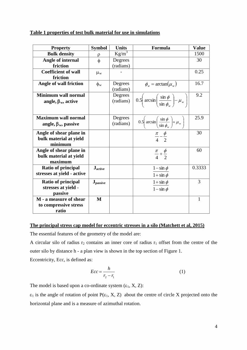
4
Table 1 properties of test bulk material for use in simulations
Property Symbol Units Formula Value
Bulk density Kg/m3 1500
Angle of internal
friction Degrees
(radians) 30
Coefficient of wall
friction w - 0.25
Angle of wall friction w Degrees
(radians) ww arctan 16.7
Minimum wall normal
angle, w, active
Degrees
(radians)
w
w
sin
sinarcsin5.0
9.2
Maximum wall normal
angle, w, passive
Degrees
(radians)
w
w
sin
sinarcsin5.0
25.9
Angle of shear plane in
bulk material at yield
minimum
24
30
Angle of shear plane in
bulk material at yield
maximum
24
60
Ratio of principal
stresses at yield - active
Jactive
sin1
sin1
0.3333
Ratio of principal
stresses at yield -
passive
Jpassive
sin1
sin1
3
M - a measure of shear
to compressive stress
ratio
M 1
The principal stress cap model for eccentric stresses in a silo (Matchett et al, 2015)
The essential features of the geometry of the model are:
A circular silo of radius r2 contains an inner core of radius r1 offset from the centre of the
outer silo by distance h - a plan view is shown in the top section of Figure 1.
Eccentricity, Ecc, is defined as:
12 rr
hEcc
(1)
The model is based upon a co-ordinate system (1, X, Z):
1 is the angle of rotation of point P(1, X, Z) about the centre of circle X projected onto the
horizontal plane and is a measure of azimuthal rotation.

5
X is the x co-ordinate of the azimuthal principal stress path projected onto the horizontal
plane as a circle of radius R1, where the circle cuts the x-axis. In 3-d space the stress path is
elliptical. The circle X also represents a constant arc angle, 2: the angle between the line of
action of principal stress 3 and the vertical plane. 2 varies from c at the annulus core to w
at the silo wall.
3 is the slope of the plane along which 2 acts, as seen from the direction of 1.
Z is the z co-ordinate of the principal stress cap at the inner core
At point P(1, X, Z), a set of local Cartesian co-ordinates (x1, x2, x3) coincide with directions
of principal stresses typical principal stress surface is shown in the lower section
of Figure 1 with local axes and principal stresses at point P marked.
acts towards the outer wall (along the -line, Matchett et al(2015))
2 acts azimuthally along the elliptical stress path in 3-d space which projects horizontally as
the X-line
3 acts normally to the principal stress cap surface(along the -line, Matchett et al(2015))
Three partial differential equations in the principal stresses were than determined from force
balances:
3222
2132
2
3
13
12
3
11
2222
1
tancoscoscos
Z
w
XRgR
DZ
D
XR
R
XE
Z
wR
Z
w
XR
(2)
222
222
3
23
22
1
22
21
31
1
121
1
21
222
222
3
23
22
1
22
21
31
1
21
sincoscos
coscos
sincoscos
cos
Z
w
XgR
DZ
D
X
R
Z
w
XE
R
R
Z
w
X
w
R
XX
or
Z
w
XgR
DZ
D
X
R
Z
w
XE
R
R
Z
w
X
w
R
DX
D
(3)

6
22
1
32
1
22
32
1
1
2
23
3
3
31
3
3
13
3
22
1
32
1
22
32
1
1
2
23
3
3
3
coscos
1
coscoscoscos
coscos
1
coscos
Z
wg
Z
w
RZ
w
R
R
W
Z
w
RDZ
DX
XDZ
DX
XZ
or
Z
wg
Z
w
RZ
w
RR
W
Z
w
RDZ
D
(4)
These were integrated numerically.
The reader is again referred to the previous paper for details, Matchett et al(2015)
Positive features of the model include:
The model is based upon rigorous, true 3-dimensional forces balances in orthogonal,
curvilinear co-ordinates, subject to the assumption of a smooth principal stress cap.
It works in principal stress space, which eliminates the need to account for shear
stresses.
The resultant numerical algorithms are relatively simple to implement, and outputs are
easy to understand and visualise.
Solutions can be obtained and analysed quickly, with a run taking about 5-10 minutes
The model is a direct extension of previous work by Janssen and Enstad
The limitations are:
The bulk material is assumed to be a rigid-plastic solid.
It is steady state and cannot predict inertial effects or model motion.
The model cannot predict contraction/dilation effects.
The principle stress cap geometry cannot be easily determined, except at limiting
conditions. It must be assumed "a priori".
Only the region of fully developed principal stress can be modelled, between the
surcharge at the top of the silo and the silo base(Matchett et al, 2015)
The lack of physical data for internal stresses makes the setting of boundary conditions very
challenging. This is particularly so for the "forgotten stress": azimuthal stress 2.
In the previous paper, the x-axis(1=0) was used as the spine of the solution. Whilst little is
known of 2, it is possible to infer 1 values and their derivatives at core and wall. These
values were used to interpolate intermediate values of 1 between the core and the wall(Xmin

7
to Xmax) along the line at 1=0. The differential equation for 1(equation 3) was then
transposed to find values of 2 along the spine. These values formed boundary conditions for
subsequent integration of the equation in 2(equation 2).
Conditions at the wall(subscript w) were fixed to give a Janssenian response(Janssen, 1895)
in a symmetrical silo(Ecc=0, equation 1):
)(:
)(:
)(:
32121
max
313
max
311max
cKX
XX
bX
XX
aKXX
www
w
www
(5)
These conditions were used along the spine, even in asymmetrical silos. Conditions along the
spine are similar to those of a symmetrical silo in that 3=0 and it is a line of symmetry.
Equations 5 represent a logical and successful attempt(Matchett et al, 2015) to reconcile
experimental observation, existing theory and the present model. However, there was
possibly an excess of fitted constants, as 1 and 2 were considered to be independent
parameters in the original paper(Matchett et al, 2015). They are problematic: they may be
material properties; particle shape dependent; silo wall properties; wall -particle interactions
or even an artifact of the model itself. Their values have been previously fixed empirically.
A simple model is proposed to eliminate one of these constants.
Consider volumetric strain at the wall - w
wwww eee 321 (6)
where eiw is the strain in direction xi at the wall.
If strain at the wall always consists of slip along the wall, it can be postulated that:
0w (7)
Now, let strain increment be proportional to stress increment:
0321 wwww (8)
Dividing by X and taking the limit, at the wall:
XXX
321
From equation 5(b) & (c)
XK ww
2
1
12
1

8
If the system at the wall is considered as a plane stress system in the 1-3 plane, then
azimuthal strains may be considered negligible along the line 1=0, which is a plane of
symmetry:
wK
12
(9)
Equation 9 will be used throughout this paper.
The equation is a simplification and other models might be proposed as further information
becomes available, for example in a situation with contraction/dilation in the wall region,
then equation 7 would not apply and would be modified to include .0w
The Enstad Core and 1 continuity
The core/annulus boundary is a vertical surface at X=Xmin; R1=r1 - see Figure 2.
Annulus principal stress 1 has value 1c and makes angle c with the horizontal. Across the
interface in the core, principal stress 1 has value 1core and makes angle core with the
horizontal.
1c is a boundary condition for 1 at the core/annulus interface, and is a key feature of 1-
interpolation along the line 1=0 through the annulus, Matchett et al(2015).
It is necessary to reconcile the two stress systems. There are a number of approaches to
modelling the stress interactions at the core-annulus boundary. Two methods will be
considered in this paper.
In the first instance, a method termed 1 continuity will be used, in which the 1 plane is
assumed to have continuity across the interface. This implies that:
ccore
ccore
11
(10)
This can be applied to a plane core:
0 ccore (11)
A value of core>0 results in an Enstad core (Enstad, 1975):
0: coreccore (12)
Stresses within the core can be found from a vertical force balance, dependent upon
assumptions made about the core.
For a plane core:
9
corecorecorecorecore
core
core
TJJ
gdZ
d
1
0
31
3
(13)
An Enstad core can be modelled as:
corecorecorecorecore
corecorecorecore
TJJ
rg
dZ
d
1
cossin2
31
1
1
3
(14)
A system of boundary conditions along the line 1=0 can now be specified for the 1-
interpolation method:
wwwww
c
XXKrRXX
rRXX
121
313
3121max
1111min
1
::::
::
:0
(15)
Equation 15 consists of 1 core and 3 wall boundary conditions. Other forms of boundary
condition are possible along the x-axis, but there is clearly a danger of over-specification of
boundary conditions in this approach: more boundary conditions than the partial differential
equations merit. Implicit in over-specification is the tendency to impart whatever properties
are desired, into the equations.
Equations 13 and 14 assume uniformity of stress across the core, but more sophisticated
models would be possible.
Core-annulus interactions: The Common Interfacial Plane (CIP)
The second model of interaction considered in this paper is one in which the common plane is
not coincident with the planes of principal stress or the core wall. This has been termed the
Common Interfacial Plane method, or CIP method.
Assume that the 1-3 stress system may be treated as a plane stress system, and the stresses
may be analysed by Mohr circles. The normal to this plane is a horizontal, circle and is the
line if action of principal stress 2.
The common plane of the two systems is at angle 1 to 1c and 2 to 1core - see Figure 2. This
is represented on a Mohr circle diagram in Figure 3. This is for a case of passive stress in the

10
core and active stress at the annulus wall. Usually, 1core and 3core are know, as is 3c-
equations 13 & 14. The aim is to find 1c and 1, by the method shown below. Equivalent
equations for other states of stress in the core and at the annulus can easily be derived.
1c acts as a boundary condition in the 1-interpolation method, as shown in equation 15
The common plane has shear stress c and normal stress c - see Figure 3
From Figure 3:
22
12
2
ccore
(16)
and
2
2
2
2
13
31
31
31
cc
ccc
corecorecore
corecorecore
qc
p
q
p
12 2sin2sin corecc qq (17)
12 2cos2cos corecoreccc qpqp (18)
Equations 17 and 18 can be solved numerically, using a number of approaches. We used
substitution followed by successive approximation, with constraints to limit the solution for
1 within the range 0- and that c lies in the appropriate range of values, in this case, 1c
should lie between 1core and 3core.
The CIP approach allows a discontinuity between the core and the annulus, in both stresses
and stress directions.
Comparisons of Internal Principal Stress Structures
Our original paper modelled a completely filled silo section with an off-centre centre-of-
stress. The boundary conditions imposed produced a Janssen-like wall normal stress response
(Matchett et al, 2015). However, there were problems with the internal stress distributions
around the centre-of-stress. Whilst the boundary conditions imposed continuity in 1 and 2
at the centre-of-stress, there were problems with "vertical" stress 3: the values of 3 were not
constant at the centre-of-stress, but varied with azimuthal parameter 1, which is conceptually
difficult for a core that has become a single point. There was a large, excessive peak in value

11
of 3, around 1=0, which increased with depth and eccentricity. The core was therefore
referred to as a "Virtual Core". This is a name, rather than an explanation.
Table 2 Comparison of internal structure: Figures 4, 5 & 6
Bulk properties are given in Table 1
Key to notation:
VC : virtual core model(Matchett et al, 2015)
ECA : Enstad core, 1-continuity model; Active core
CIPA : Common Interfacial Plane model; Active core
ECP : Enstad core, 1-continuity model; Passive core
CIPP : Common Interfacial Plane model; Passive core
Parameter VC Plane
Core
ECA CIPA ECP CIPP
Common
Parameters
r1 (m) 0.5
r2 (m) 2
Zmax (m) 15
h (m) 1
w (degrees) 15o
Kw (-) 2
1 (m-1
-1
N 37
NX 51
NZ 1000
Individual
Values
Ecc 0.5 0.667 0.667 0.667 0.667 0.667
c - 0 7.436 7.436 7.436 7.436
core 0 0 7.436 0 7.436 0
Jcore - 0.333 0.333 0.333 3 3
Tcore 0 0 0 0 0 0
It was suggested that a finite core may alleviate, or remove the peaks in 3 around the core
(Matchett et al, 2015). Therefore, a system has been modelled with a finite core, with
conditions shown in Table 2, using the 1-continuity and CIP models of core-annulus
interaction described above - equations 10-18.
The outputs of the models have been plotted as wall normal stress versus Cartesian value z, in
Figures 4a & 4b. Figure 4a compares models with an active core: Virtual Core versus 1-

12
continuity versus CIP. Figure 4b compares active and passive cores for the 1-continuity and
CIP models.
The wall normal stress responses are all Janssenian. Furthermore, the nature of internal stress
model does have an effect on wall normal stress, however, with the exception of the CIP
passive simulation at 1=0, differences are relatively small, with a range of 5.4*104-7*10
4 Pa.
The responses are not significantly different such that the internal stress pattern could be
deduced simply from the wall normal stress data.
The effects of the core model upon internal stress are shown in Figures 5a and 5b, where
Figure 5a shows the variation in principal stress 3 along the line at 1=0 (positive x-axis),
and Figure 5b shows the variation along the line at 1=180o (along the x-axis for negative
values of x).
The peak in 3 in the Virtual Core model can be seen disappearing vertically off the graph in
Figure 5a. The Plane Core model has moved the peak to the edge of the core. It has a higher
magnitude than the Virtual Core model.
The 1-continuity and CIP have greatly reduced the peak magnitude along the 1=0 line, but
there remains a discontinuity in 3 at the core wall.
Figure 5b shows the discontinuity in 3 at 1=180o.
Therefore, the 1-continuity and CIP models have brought peaks in 3 down to reasonable
values, but the discontinuities remain.
The 1-continuity model preserves continuity in 1, as the name suggests, but has
discontinuity in 2 and 3. The CIP model gives discontinuity in all 3 principal stresses at the
core.
Principal stress discontinuities would be acceptable in situations where the core was expected
to be a different stress regime to the rest of the silo: incipient coreflow and coreflow.
However, for a settled, filled silo, it would be difficult to argue why there should be
discontinuity at any particular point, unless there were a history or some other justification.
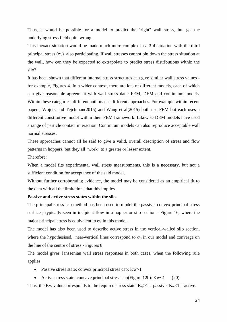
Two other effects of structure upon stress are shown in Figures 6 & 7. Figure 6 shows the
effects of core radius r1, and Figure 7 shows the effects of eccentricity (Ecc) upon wall
normal stress.
As core radius (r1) and eccentricity (Ecc) increase, the wall normal stress decreases, as shown
by the stress at a depth of 10m. There is also a tendency for azimuthal variation to increase
with an increase in r1.

13
If a set of experimental wall normal stress data were given for a filled silo, a model could be
made to fit that data by changing r1 or Ecc, or both. Again, it is impossible to relate wall
normal stress data uniquely to an internal principal stress structure within the silo.
The reverse stress cap and active stress
The traditional picture of the stress state in the silo part of a storage vessel, is one of near-
vertically aligned principal stress paths, converging on the centre-line of the silo, see Fayed
and Otten, 1997, page 409 and Figure 8a. This is associated with an active state of stress in
the silo section of the hopper. The near-vertical stress lines are equivalent to 3 in our model -
equations 2, 3 & 4. Such a situation would be equivalent to a concave surface of the principal
stress cap - Figure 8b.
Principal stress data for such a simulation are shown in Figure 9. Wall stresses are given in
Figure 10.
Clearly, the principal stress cap model is able to describe active, concave stress cap systems,
as well as the convex, passive systems more usually modelled, Enstad(1975). The radii R2 are
negative, hence the concave, rather than convex principal stress surface. Furthermore, in
order to get a Janssenian wall normal stress response, it is necessary that the stress field be
active, in particular Kw<1.
The converse applies to the passive, convex system in which Kw>1 for a Janssenian response.
As far as the authors are aware, this is the first time that an active, concave principal stress
cap system has been explicitly modelled.
Yield and friction criteria
The core stress parameters Jcore and Tcore, plus the wall principal stress ratio Kw impose
principal stress ratios at the boundaries of the system. However, the parameter Kw only
operates at the wall at 1=0, as part of the 1 interpolation procedure - Figure 5. Throughout
the rest of the material in the silo, there are no restrictions to stress ratios: stresses are
determined purely by the force balances - equations 2-4. Therefore, stresses may exceed
frictional and yield limits, because of the lack of constraint within the model, and it is
necessary to test the outputs against yield criteria.
Three types of test will be presented in the following section:
i) principal stresses in tension
ii) Wall Yield Function - WYF
iii) Conical Yield Function - CYF

14
i) Principal Stresses in Tension
Non-cohesive materials cannot support principal stresses in tension. Even for cohesive
materials, the tensile strength of a bulk solid is relatively small, and so principal stresses in
tension cannot exceed to tensile strength. Hence for principal stress i (i=1, 2, 3)
corei T (19)
Therefore, any simulation that produces excessive negative stresses in any of the principal
stresses can be rejected as non-viable. The material would deform, even if the stress state
could come to exist in the first place.
The mechanics of this test will be demonstrated with reference to two of the simulations in
Figure 4b: Common Interfacial Plane, active core (CIPA); and Common Interfacial Plane,
passive core (CIPP).
Apart from 1=0 for CIPP, the wall stress data are very similar. The principal stress
distributions across a principal stress cap can be extracted from the data, and data for 2 at
depth (Zo-Z)=15m are shown in Figure 11: CIPA(active core) in Figure 11a and CIPP(passive
core) in Figure 11b. There are clearly large areas of the stress cap for the passive core that are
negative (in tension) and hence non-viable.
The difference in internal principal stress structure(active or passive) could not be deduced
from the wall friction data - Figure 4b, although CIPP at 1=0 is an outlyer. Furthermore, an
apparently benign wall stress distribution prediction (CIPP) can hide an unfortunate internal
structure.
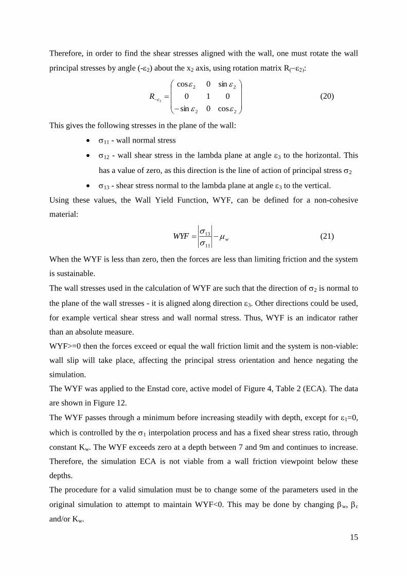
ii) Wall Yield Function - WYF
Wall shear stresses vary azimuthally and with depth - Figures 10a-c, for example. If an
appropriate ratio of shear stress to normal stress exceeds limiting wall friction, then the
material will deform and slide along the wall. Hence, the stress structure is not sustainable. A
wall friction test will be proposed, as follows:
In order to transpose from original axis system (x, y, z) to a system aligned with the direction
of principal stresses (x1, y1, z1) the following rotations of axes must be made, in the order
stated below - see Figure 1:
1. Rotate anticlockwise by angle 1 about the z-axis (axis 3)
2. Rotate clockwise by angle -3 about the x-axis (axis 1)
3. Rotate anticlockwise by angle 2 about the y-axis (axis 2)
15
Therefore, in order to find the shear stresses aligned with the wall, one must rotate the wall
principal stresses by angle (-2) about the x2 axis, using rotation matrix R(:
22
22
cos0sin
010
sin0cos
2
R (20)
This gives the following stresses in the plane of the wall:
11 - wall normal stress
12 - wall shear stress in the lambda plane at angle 3 to the horizontal. This
has a value of zero, as this direction is the line of action of principal stress 2
13 - shear stress normal to the lambda plane at angle 3 to the vertical.
Using these values, the Wall Yield Function, WYF, can be defined for a non-cohesive
material:
wWYF
11
13 (21)
When the WYF is less than zero, then the forces are less than limiting friction and the system
is sustainable.
The wall stresses used in the calculation of WYF are such that the direction of 2 is normal to
the plane of the wall stresses - it is aligned along direction 3. Other directions could be used,
for example vertical shear stress and wall normal stress. Thus, WYF is an indicator rather
than an absolute measure.
WYF>=0 then the forces exceed or equal the wall friction limit and the system is non-viable:
wall slip will take place, affecting the principal stress orientation and hence negating the
simulation.
The WYF was applied to the Enstad core, active model of Figure 4, Table 2 (ECA). The data
are shown in Figure 12.
The WYF passes through a minimum before increasing steadily with depth, except for 1=0,
which is controlled by the 1 interpolation process and has a fixed shear stress ratio, through
constant Kw. The WYF exceeds zero at a depth between 7 and 9m and continues to increase.
Therefore, the simulation ECA is not viable from a wall friction viewpoint below these
depths.
The procedure for a valid simulation must be to change some of the parameters used in the
original simulation to attempt to maintain WYF<0. This may be done by changing w, c
and/or Kw.
16
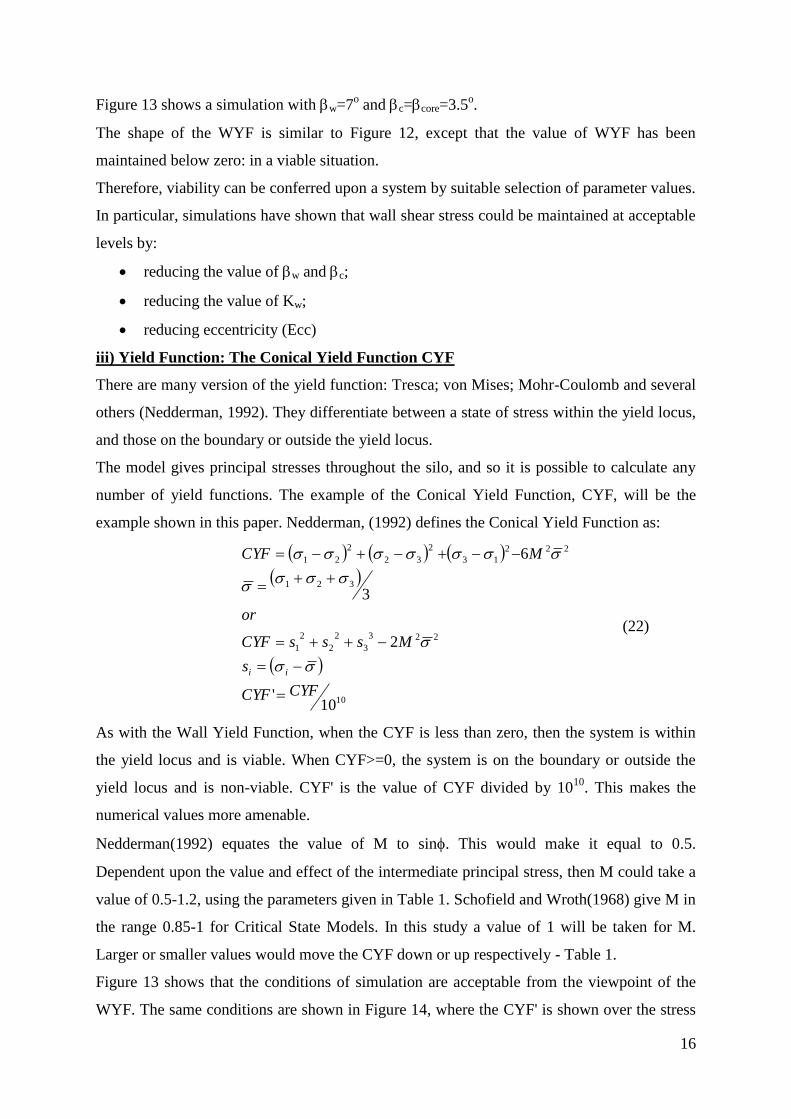
Figure 13 shows a simulation with w=7o and c=core=3.5
o.
The shape of the WYF is similar to Figure 12, except that the value of WYF has been
maintained below zero: in a viable situation.
Therefore, viability can be conferred upon a system by suitable selection of parameter values.
In particular, simulations have shown that wall shear stress could be maintained at acceptable
levels by:
reducing the value of w and c;
reducing the value of Kw;
reducing eccentricity (Ecc)
iii) Yield Function: The Conical Yield Function CYF
There are many version of the yield function: Tresca; von Mises; Mohr-Coulomb and several
others (Nedderman, 1992). They differentiate between a state of stress within the yield locus,
and those on the boundary or outside the yield locus.
The model gives principal stresses throughout the silo, and so it is possible to calculate any
number of yield functions. The example of the Conical Yield Function, CYF, will be the
example shown in this paper. Nedderman, (1992) defines the Conical Yield Function as:
10
223
3
2
2
2
1
321
222
13
2
32
2
21
10'
2
3
6
CYFCYF
s
MsssCYF
or
MCYF
ii
(22)
As with the Wall Yield Function, when the CYF is less than zero, then the system is within
the yield locus and is viable. When CYF>=0, the system is on the boundary or outside the
yield locus and is non-viable. CYF' is the value of CYF divided by 1010
. This makes the
numerical values more amenable.
Nedderman(1992) equates the value of M to sin. This would make it equal to 0.5.
Dependent upon the value and effect of the intermediate principal stress, then M could take a
value of 0.5-1.2, using the parameters given in Table 1. Schofield and Wroth(1968) give M in
the range 0.85-1 for Critical State Models. In this study a value of 1 will be taken for M.
Larger or smaller values would move the CYF down or up respectively - Table 1.
Figure 13 shows that the conditions of simulation are acceptable from the viewpoint of the
WYF. The same conditions are shown in Figure 14, where the CYF' is shown over the stress

17
cap at depth (Zo-Z) of 15m, in X-1 space. The CYF' exceeds zero in a region around the core
for 1 in the range 50o to 180
o. Clearly, even though WYF criteria have been met, CYF
criteria have not been met over the whole of the principal stress cap at a depth of 15m.
Some of the information in Figure 14 can be condensed into a single parameter: the Principal
Stress Cap Yield Quotient, or YQ:
YQ = the fraction of cells in a principal stress cap array in X-space in which the CYF is
greater than zero
(23)
Figure 15 shows YQ as a function of depth (Zo-Z) for a number of simulations, demonstrating
effects of eccentricity (Ecc) and wall normal angles. See Table 3 for details.
Table 3 Details of conditions for the simulations in Figure 15
Simulation r1
(m)
r2
(m)
Ecc
(-)
h
(m)
w
(deg)
c=core
(deg)
Kw 1
Basecase Figs 13 & 14 0.5 2 0.667 1 7 3.5 2 -1
Basecase: Ecc varied 0.5 2 var var 7 3.5 2 -1
Basecase: half angles 0.5 2 0.667 1 3.5 1.75 2 -1
Concave 1 0.5 2 0 0 -7 0 0.95 -1
Concave 2 0.5 2 0 0 -5 0 0.95 -1
Figure 15 shows that the YQ remains below zero until a critical depth (Zo-Z) is reached. This
critical depth decreases as eccentricity increases and as wall angle w increases. Once the
critical depth is exceeded then the YQ increases steadily with depth.
Above a certain Eccentricity(see Ecc=0.8 in Figure 15), the system can never sustain a stress
system within the yield locus for the conditions modelled here.
The preceding argument applies equally to concave yield surfaces - Figures 8, 9 & 10.
The analysis implies that deep beds in completely filled silos with fully developed stress
systems cannot support high stress eccentricities or relatively large wall and core angles. This
is supported by both the 1-continuity and CIP core annulus interaction algorithm outputs.
The data from the Virtual Core model in the first paper (Matchett et al, 2015) can also be

18
interpreted to give the same conclusion: deep beds with high eccentricity and/or large wall
normal angles give excessive stress peaks at the Virtual Core, which are not viable.
The magnitudes of the descriptors "deep" silo and "relatively large angles" can be quantified
by the model.
Accepting the yield limitation criteria upon Ecc and w within a filled silo, the Virtual Core
model (Matchett et al, 2015) may be the best approach. It removes the stress continuity
problems at the core-annulus interface. However, these are replaced by the anomalies of the
Virtual Core.
Incipient core-flow and the stress switch
Incipient core-flow will now be modelled. This is the stress situation at the core yield limit as
the core is about to start to flow. It does not involve inertial terms or contraction/dilation
effects. It is assumed that there is no immediate flow in the annulus.
There are several ways in which incipient flow may be modelled within this eccentric stress,
silo simulation, and two will be considered here:
1 continuity at the core-annulus interface
The use of the Common Interfacial Plane algorithm (CIP) at the interface
At incipient flow, it is generally accepted that the core, which is about to flow, will be in a
state of passive stress with the arc normal angle equal its limiting passive value: 60o in this
case - Table 1.
The normal angle at the core (c=core) of 60o is greater than the maximum wall normal angle
of 25.9o - Table 1. This enforces a concave principal stress surface system into the silo -
Figures 8, 9 & 10, for the 1 continuity model. Therefore, Kw must be active and have a
value less than 1. This approach implies yield or positive value of CYF at the core and the
annulus wall.
The CIP model can allow core to be 60o, whilst c and w may take other values, due to the
discontinuity at the core-annulus interface.
Two simulations have been run to compare the two methods of modelling incipient flow. The
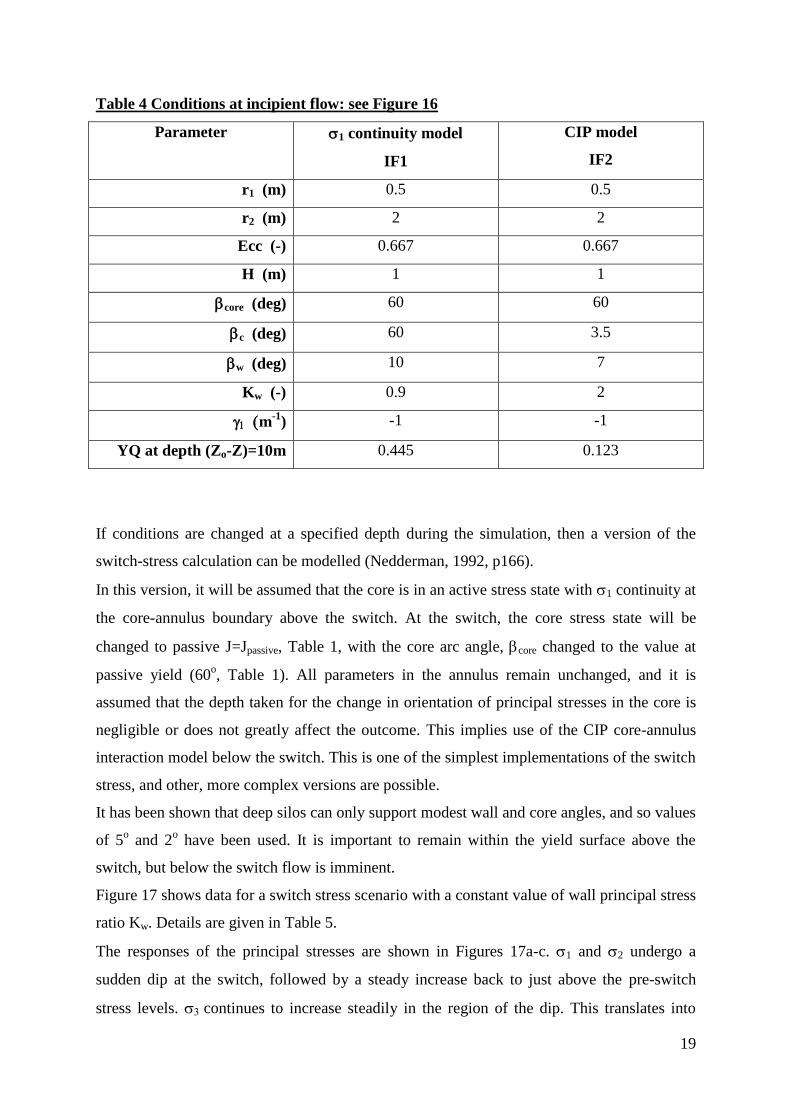
conditions are shown in Table 4.
Wall normal and wall vertical shear stresses for the conditions in Table 4 are shown in
Figures 16a & 16b respectively. The wall stresses are quite different, both quantitatively and
qualitatively. In these circumstances, the choice of internal principal stress geometry has a
great effect upon measured wall stresses.
19
Table 4 Conditions at incipient flow: see Figure 16
Parameter 1 continuity model
IF1
CIP model
IF2
r1 (m) 0.5 0.5
r2 (m) 2 2
Ecc (-) 0.667 0.667
H (m) 1 1
core (deg) 60 60
c (deg) 60 3.5
w (deg) 10 7
Kw (-) 0.9 2
m-1
) -1 -1
YQ at depth (Zo-Z)=10m 0.445 0.123
If conditions are changed at a specified depth during the simulation, then a version of the
switch-stress calculation can be modelled (Nedderman, 1992, p166).
In this version, it will be assumed that the core is in an active stress state with 1 continuity at
the core-annulus boundary above the switch. At the switch, the core stress state will be
changed to passive J=Jpassive, Table 1, with the core arc angle, core changed to the value at
passive yield (60o, Table 1). All parameters in the annulus remain unchanged, and it is
assumed that the depth taken for the change in orientation of principal stresses in the core is
negligible or does not greatly affect the outcome. This implies use of the CIP core-annulus
interaction model below the switch. This is one of the simplest implementations of the switch
stress, and other, more complex versions are possible.
It has been shown that deep silos can only support modest wall and core angles, and so values
of 5o and 2
o have been used. It is important to remain within the yield surface above the
switch, but below the switch flow is imminent.
Figure 17 shows data for a switch stress scenario with a constant value of wall principal stress
ratio Kw. Details are given in Table 5.
The responses of the principal stresses are shown in Figures 17a-c. 1 and 2 undergo a
sudden dip at the switch, followed by a steady increase back to just above the pre-switch
stress levels. continues to increase steadily in the region of the dip. This translates into

20
wall normal stress responses, as shown in Figure 17d. There are azimuthal variations in
stresses, which increase as eccentricity(Ecc) increases.
Table 5 Conditions for switch simulation in Figures 17 and 18
Figure 17 Figure 18 Figure 19
Core radius r1 (m) 0.5 0.5 0.5
Silo radius r2 (m) 3.0 3.0 3
Eccentricity Ecc 0.75 0.75 0.95
Offset h (m) 2.25 2.25 2.375
w (deg) 5 5 5
c (deg) = core above switch 2 2 2
core (deg) below switch 60 60 60
1 -1.5 -1.5 -2
Above switch
Jcore 0.5 0.5 0.333
Tcore 0 0 0
Kw 2.1 2.1 1.1
Below switch
Jcore 2.5 2.5 3
Tcore 0 0 0
Kw 2.1 2.5 3
Zmax (m) 30 30 30
Zswitch (m) 5 5 5
At the wall, at 1=0 and for all values of 1 at eccentricity, Ecc=0, then 1 is directly related to
3 through equation 5a. Thus, if the switch causes little variation in 3 - Figure 17c, then little
change can be expected in 1, because of equation 5a.
It can be argued that as the state of stress changes at the core, during the switch, then an
equivalent change might be expected at the wall, with an increase in Kw below the switch.
This has been modelled in Figures 18, for conditions shown in Table 5, with an increase in
Kw from 2.1 to 2.5 at the switch. The drop in stresses at the switch is no longer present, and
the stress increases at switch are more pronounced in and wall normal stress. 3
increases gradually at the switch, as in Figure 17. However, the magnitude of the switch

21
stress can now be controlled by the programmer through the change in parameter Kw at
switch. The magnitude of change could thus be calibrated by comparison with appropriate
experimental data.
It is interesting to consider an extreme switch stress at conditions close to the maximum
possible. Conditions are given in Table 5. the changes in Jcore and Kw are the maximum
possible. Wall normal stress variation with depth is shown in Figure 19 for a system with a
high eccentricity: Ecc=0.95. Under these conditions, the switch can double wall normal stress
(at 1=0). There are also large azimuthal normal stress variations.
Several other implementations of a switch stress are possible, including versions in which the
annulus as well as core stress states change. Problems include:
how the stress states change within the core and annulus
how to model the transition from one stress state to the other
The implementation presented herein does give a methodology for quantifying the switch
stress in eccentric stress systems, however imperfect.
Discussion
Overview: positive features -
This model is one of the few, perhaps very few dedicated models of eccentric stress in silos
and hoppers. It is a true 3-dimensional model, based upon the principal stress cap approach of
Enstad: Enstad(1975), Matchett et al(2015). The assumed model of principal stress geometry
is such that it could be approximated to a wide range of shapes, provided that the principal
stress surfaces are smooth and there are no discontinuities within the annulus.
The model can describe the perceived features of stress systems in a silo:
Janssenian wall stresses: Figures 4 and Matchett et al(2015)
Passive stress systems, Figures 4-7, Matchett et al(2015)
Active stress state, Figures 8, 9 & 10
Determination of yield conditions at the wall and internally and consideration
of whether stress states remain within the yield surface, Figures 11-15
Incipient coreflow - Figures 16
Switch stresses - Figures 17, 18, 19
22
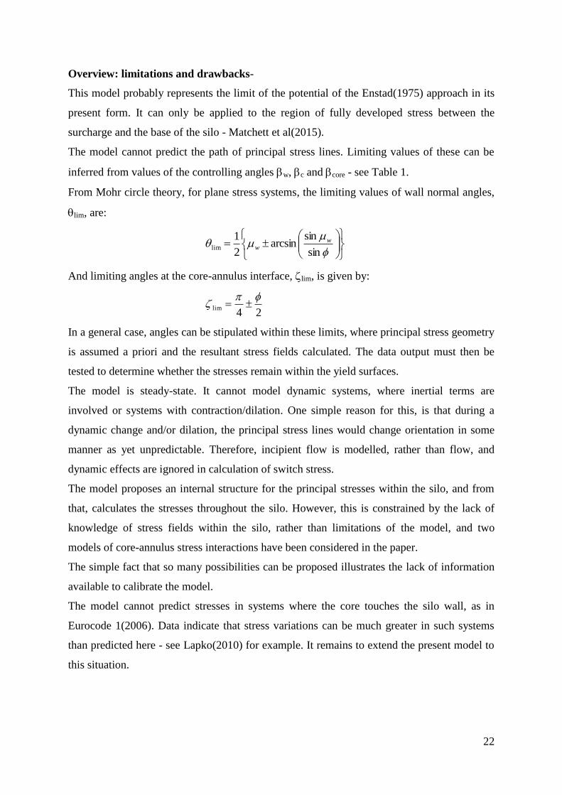
Overview: limitations and drawbacks-
This model probably represents the limit of the potential of the Enstad(1975) approach in its
present form. It can only be applied to the region of fully developed stress between the
surcharge and the base of the silo - Matchett et al(2015).
The model cannot predict the path of principal stress lines. Limiting values of these can be
inferred from values of the controlling angles w, c and core - see Table 1.
From Mohr circle theory, for plane stress systems, the limiting values of wall normal angles,
lim, are:
sin
sinarcsin
2
1lim
ww
And limiting angles at the core-annulus interface, lim, is given by:
24
lim
In a general case, angles can be stipulated within these limits, where principal stress geometry
is assumed a priori and the resultant stress fields calculated. The data output must then be
tested to determine whether the stresses remain within the yield surfaces.
The model is steady-state. It cannot model dynamic systems, where inertial terms are
involved or systems with contraction/dilation. One simple reason for this, is that during a
dynamic change and/or dilation, the principal stress lines would change orientation in some
manner as yet unpredictable. Therefore, incipient flow is modelled, rather than flow, and
dynamic effects are ignored in calculation of switch stress.
The model proposes an internal structure for the principal stresses within the silo, and from
that, calculates the stresses throughout the silo. However, this is constrained by the lack of
knowledge of stress fields within the silo, rather than limitations of the model, and two
models of core-annulus stress interactions have been considered in the paper.
The simple fact that so many possibilities can be proposed illustrates the lack of information
available to calibrate the model.
The model cannot predict stresses in systems where the core touches the silo wall, as in
Eurocode 1(2006). Data indicate that stress variations can be much greater in such systems
than predicted here - see Lapko(2010) for example. It remains to extend the present model to
this situation.

23
Reconciling data from the model with other sources-
It was shown in our previous paper(Matchett et al, 2015) that the model can be fitted to wall
stress data from a DEM simulation. Model parameters may be adjusted empirically to give a
desired output. The reader is referred to the first paper(Matchett et al, 2015) for the data
fitting methodology.
Unfortunately, such adjustment is almost purely empirical. It has been shown that a range of
internal parameters can predict similar wall stresses, both in this paper and in the previous
one: Matchett et al(2015).
More generally, silo stress data consist of wall stress measurements. The wall stress
measurements consist mainly of wall normal stress. For a full survey see our previous paper,
Matchett et al(2015). Wall normal stress is a key parameter in the structural design of a silo,
as well as being the most widely measured of silo stress parameters and therefore features
throughout this paper.
There are few examples, if any, of measured internal stresses in silos. Added to this, the
authors do not know of any measurements of azumuthal stresses: 2 in this model. It is the
"forgotten stress" in silo modelling. This makes comparisons difficult and boundary
conditions cannot be easily formulated.
Wall stress data have been measured in a relatively large number of studies. Wall stress
measurement is a poor indicator of the principal stress orientation within the centre of the
silo. Wall stress measurements do not even give a definitive statement of principal stress
orientation at the wall, as shown below:
Consider a general situation where wall normal stress, c is measured in a plane stress
system. This single measurement tells us the following about the principal stresses - see
Figure 20, Mohr circle 1:
i) Minor principal stress min<=c
ii) Major principal stress maj>=c
This is clearly not an exact situation.
Some workers have also measured shear stress c - Figure 20. Askegaard(1988) pioneered the
use of embedded cells for this purpose, but papers presenting shear as well as normal data are
few, compared to those measuring only normal stress. These two measurements now give a
single point on the Mohr circle. But many Mohr circles could pass through that point: two
such Mohr circles are shown in Figure 20: Mohr circle 1 and Mohr circle 2.
24
Thus, it would be possible for a model to predict the "right" wall stress, but get the
underlying stress field quite wrong.
This inexact situation would be made much more complex in a 3-d situation with the third
principal stress (2) also participating. If wall stresses cannot pin down the stress situation at
the wall, how can they be expected to extrapolate to predict stress distributions within the
silo?
It has been shown that different internal stress structures can give similar wall stress values -
for example, Figures 4. In a wider context, there are lots of different models, each of which
can give reasonable agreement with wall stress data: FEM, DEM and continuum models.
Within these categories, different authors use different approaches. For example within recent
papers, Wojcik and Tejchman(2015) and Wang et al(2015) both use FEM but each uses a
different constitutive model within their FEM framework. Likewise DEM models have used
a range of particle contact interaction. Continuum models can also reproduce acceptable wall
normal stresses.
These approaches cannot all be said to give a valid, overall description of stress and flow
patterns in hoppers, but they all "work" to a greater or lesser extent.
Therefore:
When a model fits experimental wall stress measurements, this is a necessary, but not a
sufficient condition for acceptance of the said model.
Without further corroborating evidence, the model may be considered as an empirical fit to
the data with all the limitations that this implies.
Passive and active stress states within the silo-
The principal stress cap method has been used to model the passive, convex principal stress
surfaces, typically seen in incipient flow in a hopper or silo section - Figure 16, where the
major principal stress is equivalent to 1 in this model.
The model has also been used to describe active stress in the vertical-walled silo section,
where the hypothesised, near-vertical lines correspond to 3 in our model and converge on
the line of the centre of stress - Figures 8.
The model gives Janssenian wall stress responses in both cases, when the following rule
applies:
Passive stress state: convex principal stress cap: Kw>1
Active stress state: concave principal stress cap(Figure 12b): Kw<1 (20)
Thus, the Kw value corresponds to the required stress state: Kw>1 = passive; Kw<1 = active.

25
If the above rule is not applied, in both cases, wall stresses increase exponentially.
As far as the authors are aware, this is one of the first attempts to explicitly model the active
stress state, as shown in Figure 8.
Structural Implications-
The present model indicates large stress variations, both azimuthally and axially, associated
with high stress eccentricity, measured by eccentricity(Ecc) - equation 1, and large wall
normal angles w. Fortunately, in deep, filled silos, eccentricity and wall normal angle must
remain modest, in order to maintain the stresses within the yield surfaces. However, if larger
values were to occur, as a transient state, then there may be structural problems: for example
the opening of an off-centre outlet with high eccentricity - Figure 19. Unfortunately, this
model cannot describe transient situations and this must be taken into account in the
interpretation of such data
Generally, there are large azimuthal variations in wall vertical shear stress, even at modest
eccentricity and wall normal angles - for example, see Figure 16b. The resultant forces are
limited by limiting friction, but even so, some regions of the wall circumference will be at
limiting friction while others will be below this level. Wojcik and Tejchman(2015) state that
buckling is caused by wall friction(rather than normal stress), particularly during eccentric
discharge and therefore, the asymmetry of wall shear may be a critical factor.
Future Developments-
The implementation of the model is limited by lack of detailed information of the principal
stress structure within a silo. There is a vital need for experimentation. Modern stress
measurement technology should be capable of developing sensors that measure and transmit
internal stresses from within a hopper/silo system.
Experimental work needs to be supported by simulation, using FEM and DEM. One possible
approach would be to calibrate the model against internal properties taken from DEM and
FEM simulations. Such an approach would be very labour-intensive.
This modelling approach is limited by the inability to calculate and predict principal stress
lines related to the principal stress cap, rather than assuming them. It is not clear how this
could be done efficiently within the context of the model. If it were possible, it may be
feasible to model dynamic systems using the principal stress cap approach and incorporating
changes in principal stress directions with motion.
26
Conclusions
Stresses have been modelled in a silo with a finite, off-centre core within the silo, using the
principal stress cap approach.
Several types of core wall-annulus interaction are possible and two have been proposed in
this paper. A finite, Enstad core with 1 continuity and an Enstad core, with the use of CIP
Common Interfacial Plane interaction model greatly reduce the stress peak in 3, but
discontinuity at the core remain to a greater or lesser extent (Matchett et al, 2015).
Passive, convex and active, concave principal stress systems can be described by this model.
Generally, it is not possible to predict internal principal stress structure from wall stress
measurements.
The Wall Yield Function analyses and the Conical Yield Function (CYF) analyses suggest
that wall normal angle, w, and eccentricity (Ecc) must be small in deep beds i.e. deep stable
beds with high eccentricity and/or large wall normal angle are not viable.
Incipient coreflow and switch stresses have been modelled.
Implementation of the model is hindered by lack of information about the internal stress
structures of materials in silos.
References
Askegaard V., J.Munch-Andersen, 1985. Results from tests with normal and shear cells in a
medium-scale model silo,. Powder Technology, 44, 151-157
bulk-online forum, http://forum.bulk-online.com
Carson J.W., Silo Failures: case histories and lessons learned, Third Israeli Conference for
Conveying and handling of Particulate Solids, Dead Sea, Israel, May 2000
Enstad G., 1975, On the theory of arching in mass flow hoppers, Chem.Eng.Sci. 30, 1273-
1283
Eurocode 1, EN 1991-4, 2006. Action on structures - Part 4: Silos and Tanks. Brussels,
Belgium.
Fayed M.E., L.Otten, Handbook of Powder Science and Technology, 2nd
Edition, Chapman
and Hall, New York, 1997
Janssen H.A., 1895. Versuche uber getreidedruck in silozellen, Zeitschrift verein Deutsche
Inginieur, 39,1045-1049
Lapko A. 2010. Pressure of agricultural solids under eccentric discharging of cylindrical
concrete silo bin. Int.Agrophysics 24, 51-56

27
Matchett A.J., P.A.Langston, D.McGlinchey. 2015. A model for stresses in a circular silo
with an off-centre circular core, using the concept of a principal stress cap: Solutions for a
completely filled silo and comparison with DEM data. Chemical Engineering Research and
Design 93, 330-348
Nedderman R.M.(1992), Statics and Kinematics of Granular Materials, Cambridge
University Press, Cambridge, England
Ramirez-Gomez A., E.Gallego, J.M.Fuentes, C. Gonzalez-Montellano, C.J.Porras-Prieto,
F.Ayuga. 2015. Full-scale tests to measure stresses and vertical displacements in an 18.34m-
diameter steel roof silo. 106, 56-65
Sadowski A.J., J.M.Rotter, 2011. Buckling of very slender metal silos under eccentric
discharge. Engineering Structures, 33, 1187-1194
Schofield A., P.Wroth, 1968, Critical State Soil Mechanics, McGraw-Hill, New York, USA
Sielamovicz I., M.Czech, T.A Kowalewski. 2010. Empirical description of flow parameters
in eccentric flow inside a silo model, Powder Technology 198, 381-394
Sielamovicz I., M.Czech, T.A Kowalewski. 2011. Empirical analysis of eccentric flow
registered by teh DPIV technique inside a model silo, Powder Technology 212, 38-56
Sielamovicz I., M.Czech, T.A Kowalewski. 2015. Comparative analysis of empirical
descriptions of eccentric flow in silo model by the linear and non-linear regressions, Powder
Technology 270, 393-410
Sondej M., P.Iwicki, J.Tejchman, M.Wojcik. 2015. Critical assessment of Eurocode approach
to stability of metal cylindrical silos with corrugated walls and vertical stiffeners. Thin-
Walled Structures. 95, 335-346
Wojcik M., J.Tejchman. 2015. Simulation of buckling process of cylindrical metal silos with
flat sheets containing bulk solids. Thin-Walled Structures. 932, 122-136
Yin Wang , Y.Lu, J.Y.Ooi. 2015. A numerical study of wall pressure and granular flow in a
flat-bottomed silo. Powder Technology. 282, 43-54
Notation
SYMBOL DESCRIPTION UNITS
a1 Relates projected circle radius R1 to X '111 aXaR -
a1’ Constant relating R1 to X – see a1 m
a2 Differential of projected circle centre
XO
a X
2 -
D D/DX and D/DZ are differentials along the principal stress paths
for changes in X & Z respectively

28
e1 Angle used in the calculation of R2 rad
E Factor relating rotation in the horizontal plane to rotation on the -
plane
-
h Inner circle offset m
-
k Ratio of wall vertical to normal stress: Janssen model -
Kw Ratio of at the wall -
M Conical Yield Function parameter -
r1 Inner circle radius m
r2 Outer circle (silo) radius m
R1 Radius of projected horizontal circle of principal stress path m
R2 Radius of principal stress cap at a general point m
R20 Value of R2 at m
R2 Value of R2 at m
w1 Arc length along -line, seen as
Xw
1
m
w2 Arc length along -line, seen as
Zw
2
m
x x-axis co-ordinate m
X Intercept of projected horizontal surface with x-axis m
Xo Minimum value of X m
Xmax Maximum value of X m
x1, x2, x3 Local Cartesian co-ordinates coincident with directions of
principal stress
-
y y-axis co-ordinate m
z z-axis co-ordinate m
Z Value of z for the inner radius of the principal stress cap m
Zo Value of Z at the point of boundary conditions m
c Angle of circular arc to normal at inner core rad
w Angle of circular arc to normal at wall rad
Angle from x-axis in the horizontal plane rad
Angle from the vertical in the x-z plane at , rotated along the
elliptical, principal stress path
rad
Angle from the vertical – slope of the principal stress cap surface
as seen from
rad
Slope of principal stress, 3 at the wall Pa/m
Slope of principal stress, 1 at the wall
Angle of internal friction. A nominal value of 30o has been used. rad

29
Characteristic slope of principal stress path ellipse when projected
onto the x-z plane
rad
w Coefficient of wall friction. A nominal value of 0.3 has been used. -
Surcharge friction factor -
lim Limiting value of wall arc angle rad
lim Limiting value of plane of yield rad
Angle of -line to x-axis on the horizontal plane rad
Angle of -line to vertical – principal stress path for changes in Z rad
Bulk density of the bulk solid in the silo Kg/m3
Principal stress in x1 direction Pa
Principal stress in x2 direction Pa
Principal stress in x3 direction Pa
Figures
Figure 1 The principal stress cap and essential structure of the principal stress cap,
eccentric silo model
Figure 2 Core-annulus interaction for the Common Interfacial Plane model - CIP model
Figure 3 Mohr circles for the Common Interfacial Plane model: Mohr circles of the core
wall and annulus wall
Figure 4 Effects of internal structure on wall normal stress. Variation of wall normal
stress with depth, as measured by z (Cartesian)
See Tables 1 & 2 for conditions
Figure 4a: different core models
Figure 4b: active and passive cores
VC : virtual core model(Matchett et al, 2015)
ECA : Enstad core, 1-continuity model; Active core
CIPA : Common Interfacial Plane model; Active core
ECP : Enstad core, 1-continuity model; Passive core
CIPP : Common Interfacial Plane model; Passive core
Figure 5 Internal stress distributions for different core models.
See Tables 1 & 2 for details
Figure 5a: 3 variation along the X-line at 1=0o
Figure 5b: 3 variation along the X-line at 1=180o
VC : virtual core model(Matchett et al, 2015)
ECA : Enstad core, 1-continuity model; Active core

30
CIPA : Common Interfacial Plane model; Active core
ECP : Enstad core, 1-continuity model; Passive core
CIPP : Common Interfacial Plane model; Passive core
Figure 6 Effects of core radius on wall normal stress: variation in wall normal stress
with azimuthal variation 1, at depth (Zo-Z) of 10m.
Conditions as in Table 2, except:
Active core, Jcore=0.333; h=1 m throughout
Enstad core with 1-continuity.
w=8o; c=core=3
o
Figure 7 Effects of Eccentricity (Ecc) on wall normal stress: variation in wall normal
stress with azimuthal variation 1, at depth (Zo-Z) of 10m.
Conditions as in Table 2, except:
Passive core, Jcore=3; r1=0.5 m throughout
Enstad core with 1-continuity.
w=10o; c=core=3
o
Figure 8 Concave principal stress cap half-surface
r1=0.5; r2=2m; c=core=-1o; w=-10
o
Figure 8a The accepted picture of lines of major principal stress in hopper/silo
sections.
Figure 8b The shape of the principal stress cap surface
Figure 9 Principal stress surfaces in X-1 space at depth (Zo - Z) of 10m
Geometry as in Figure 8.
=1500 kg/m3; 1=-1; Kw=0.95; 2=-1/Kw; Ecc=0.5
Figure 9a 1 in X-1 space
Figure 9b 2 in X-1 space
Figure 9c 3 in X-1 space
Figure 10 Wall stresses for conditions in Figures 8 & 9
Figure 10a wall normal stress versus z
Figure 10b wall vertical shear stress versus z
Figure 10c wall horizontal shear stress
Figure 11 Principal stress 2 over the principal stress cap at depth (Zo-Z)=15m.
The conditions are given in Table 2.
Figure 11a CIPA
Figure 11b CIPP
Figure 12 Wall Yield Function (WYF) as a function of 1 and depth for the simulation
EPA in Figure 4. See Figure 2 for details
Figure 13 Wall Yield Function (WYF) as a function of 1 and depth for the simulation of
revised conditions for the ECA simulation. Conditions as in Figure 4, Table 2
and Figure 12, except:
w=7o; c=core=3.5
o

31
Figure 14 CYF' for the principal stress cap at depth (Zo-Z) of 15m. Conditions as shown
in Figure 13.
Figure 15 The Yield Quotient (YQ) for a range of simulations, including those in Figures
13 & 14. For details see Table 3.
Figure 16 Wall stresses for a silo at incipient core-flow. For conditions see Table 4
Figure 16a wall normal stress versus z
Figure 16b wall vertical shear stress versus z
Figure 17 Switch stresses in a silo section 3m radius and 30m tall: conditions shown in
Table 5
Figure 17a Principal stress 1 versus Cartesian coordinate z
Figure 17b Principal stress 2 versus Cartesian coordinate z
Figure 17c Principal stress 3 versus Cartesian coordinate z
Figure 17d Wall normal stress in the region of the switch versus Cartesian
coordinate z
Figure 18 Switch stresses in a silo section 3m radius and 30m tall with an increase in Kw
below the switch: conditions shown in Table 5
Figure 18a Principal stress 1 versus Cartesian coordinate z
Figure 18b Principal stress 2 versus Cartesian coordinate z
Figure 18c Principal stress 3 versus Cartesian coordinate z
Figure 18d Wall normal stress in the region of the switch versus Cartesian
coordinate z
Figure 19 Wall normal stress for conditions close to those of maximum magnitude
switch stress. For conditions see Table 5
Figure 19a Overall wall normal stress variation with depth with 1 (deg) as a
parameter
Figure 19b Wall normal stress in the region of the switch with 1 (deg) as a
parameter
Figure 20 Wall stress measurements - the relation between wall stress measurement,
Mohr Circles and their wider interpretation in terms of stress structure through
the silo

Figure 1 The principal stress cap and essential structure of the principal stress cap,
eccentric silo model
silo radius r2
h offset
core radius r1
x
y
azimuthal stress path projected onto horizontal plane
X (upper case): x co-ordinate of
azimuthal stress path Point P(1, X, Z)
Cartesian co-ordinates are centred on the
core, (x, y, z)
The azimuthal stress path intersects the x-
axis at X
X refers to a point P, on the projected
stress path
Angle 1 is a rotation about the centre of
circle X
x
y
z
Principal stresses at P act on the principal stress cap
surface - as shown below:
Matchett, Langston & McGlinchey, ChERD, 2015, 93,
330-348
Figure

Figure 2 Core-annulus interaction for the Common Interfacial Plane model - CIP
model
r1
CORE ANNULUS
c
core
1core
1c
Interface
core
CIP

Figure 3 Mohr circles for the Common Interfacial Plane model: Mohr circles of the core
wall and annulus wall
c c core core
CIP (c, c)
12
annulus Mohr Circle
Core Mohr Circle

Figure 4
Effects of internal structure on wall normal stress. See Tables 1 & 2 for conditions. Figure 4a: different core models
0.0E+00
1.0E+04
2.0E+04
3.0E+04
4.0E+04
5.0E+04
6.0E+04
7.0E+04
8.0E+04
0 2 4 6 8 10 12 14
wall normal stress (Pa)
z (m)
0 deg; VCA
90 deg; VCA
180 deg; VCA
0 deg; EA
90 deg; EA
180 deg; EA
0 deg; CIPA
90 deg; CIPA
180 deg; CIPA

Figure 4 Effects of internal structure on wall normal stress.
Figure 4b: active and passive cores
0.0E+00
1.0E+04
2.0E+04
3.0E+04
4.0E+04
5.0E+04
6.0E+04
7.0E+04
8.0E+04
9.0E+04
1.0E+05
0.0E+00 2.0E+00 4.0E+00 6.0E+00 8.0E+00 1.0E+01 1.2E+01 1.4E+01
wall normal stress (Pa)
z (m) (Cartesian)
0 deg EA
90 deg EA
180 deg EA
0 deg EP
90 deg EP
180 deg EP
0 deg CIPA
90 deg CIPA
180 deg CIPA
0 deg CIPP
90 deg CIPP
180 deg CIPP

Figure 5 Internal stress distributions for different core models.
See Tables 1 & 2 for details. Figure 5a: 3 variation along the X-line at 1=0o
0.0E+00
5.0E+04
1.0E+05
1.5E+05
2.0E+05
2.5E+05
3.0E+05
0 0.1 0.2 0.3 0.4 0.5 0.6 0.7 0.8 0.9 1
3 (Pa)
X (m)
Virtual Core
Plane Core
Enstad Core
CIP Core

Figure 5 Internal stress distributions for different core models.
See Tables 1 & 2 for details . Figure 5b: 3 variation along the X-line at 1=180o
0.0E+00
2.0E+05
4.0E+05
6.0E+05
8.0E+05
1.0E+06
1.2E+06
1.4E+06
0 0.1 0.2 0.3 0.4 0.5 0.6 0.7 0.8 0.9 1
3 (Pa)
X (m)
Virtual Core
Plane Core
Enstad Core
CIP Core
Figure 6 Effects of core radius on wall normal stress: variation in wall normal stress with azimuthal variation 1, at depth (Zo-Z) of
10m.
Conditions as in Table 2, except:
Active core, Jcore=0.333; h=1 m throughout
Enstad core with 1-continuity.
w=8o; c=core=3
o
0.0E+00
1.0E+04
2.0E+04
3.0E+04
4.0E+04
5.0E+04
6.0E+04
7.0E+04
8.0E+04
0 20 40 60 80 100 120 140 160 180
wall normal stress (Pa)
eta1 (degrees)
0.05
0.25
0.5
0.75
0.9

Figure 7 Effects of Eccentricity (Ecc) on wall normal stress: variation in wall normal stress with azimuthal variation 1, at depth
(Zo-Z) of 10m.
Conditions as in Table 2, except:
Passive core, Jcore=3; r1=0.5 m throughout
Enstad core with 1-continuity.
w=10o; c=core=3
o
0.0E+00
2.0E+04
4.0E+04
6.0E+04
8.0E+04
1.0E+05
1.2E+05
1.4E+05
1.6E+05
1.8E+05
2.0E+05
0 20 40 60 80 100 120 140 160 180
wall normal stress Pa
1 deg
0
0.25
0.5
0.75
0.85
0.95

Figure 8 Concave principal stress cap half-surface
Figure 8a The accepted picture of lines of major principal stress in hopper/silo
concave principal
stress cap for
an active
stress state
convex principal
stress cap in the
passive hopper
section
major
principal
stress

Figure 8b The shape of the principal stress cap surface half section; r1=0.5; r2=2m; c=core=-1o; w=-10
o
Figure 9 Principal stress surfaces in X-1 space at depth (Zo - Z) of 10m. Geometry as in Figure 8. =1500 kg/m3; 1=-1; Kw=0.95;
2=-1/Kw; Ecc=0.5.
Figure 9a 1 in X-1 space
0.0E+00
1.0E+04
2.0E+04
3.0E+04
4.0E+04
5.0E+04
6.0E+04
7.0E+04
8.0E+04
1 deg
1 Pa
X m

Figure 9b 2 in X-1 space
0.0E+00
5.0E+04
1.0E+05
1.5E+05
2.0E+05
2.5E+05
1 deg
Pa
X m
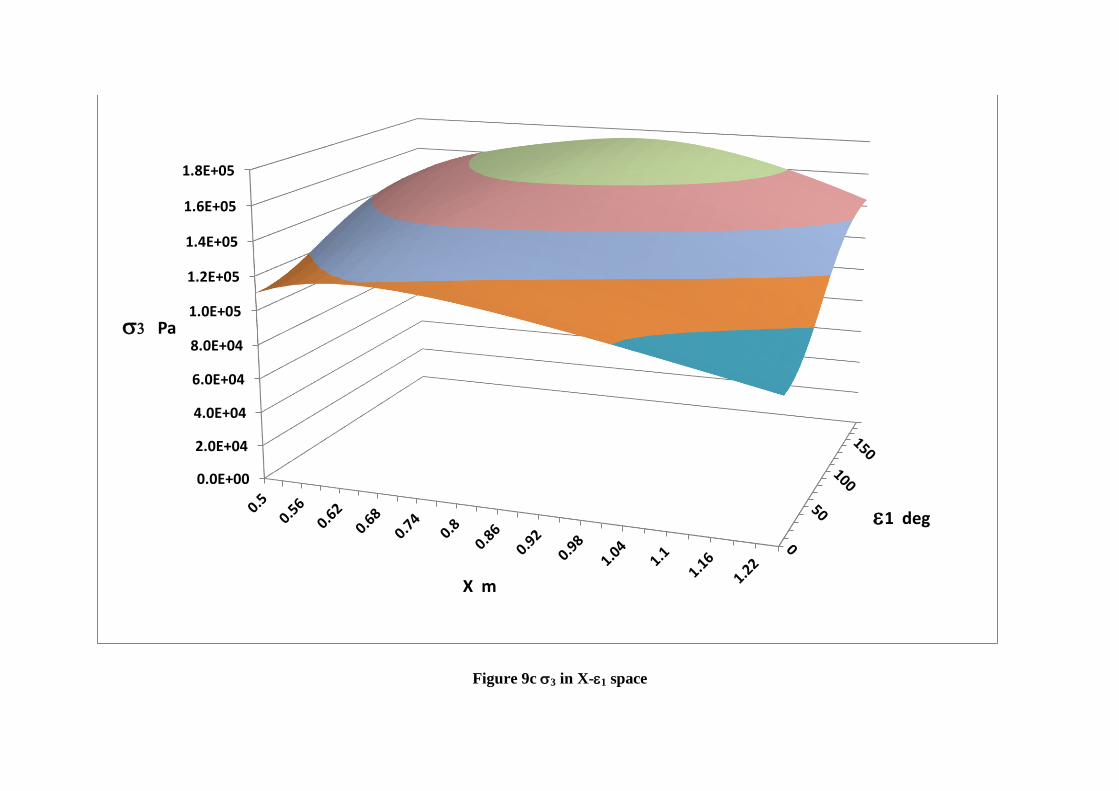
Figure 9c 3 in X-1 space
0.0E+00
2.0E+04
4.0E+04
6.0E+04
8.0E+04
1.0E+05
1.2E+05
1.4E+05
1.6E+05
1.8E+05
1 deg
Pa
X m

Figure 10 Wall stresses for conditions in Figures 8 & 9.
Figure 10a wall normal stress versus z
0.0E+00
1.0E+04
2.0E+04
3.0E+04
4.0E+04
5.0E+04
6.0E+04
7.0E+04
8.0E+04
9.0E+04
0 1 2 3 4 5 6 7 8 9 10
wall normal stress Pa
z m
0 deg
60 deg
90 deg
120 deg
180 deg

Figure 10b wall vertical shear stress versus z
-1.2E+04
-1.0E+04
-8.0E+03
-6.0E+03
-4.0E+03
-2.0E+03
0.0E+00
2.0E+03
0 1 2 3 4 5 6 7 8 9 10
wall vertical shear stress Pa
z m
0 deg
60 deg
90 deg
120 deg
180 deg

Figure 10c wall horizontal shear stress
-3.0E+02
-2.5E+02
-2.0E+02
-1.5E+02
-1.0E+02
-5.0E+01
0.0E+00
5.0E+01
0 1 2 3 4 5 6 7 8 9 10
wall horizontal shear stress Pa
z m
0 deg
60 deg
90 deg
120 deg
180 deg

Figure 11 Principal stress 2 over the principal stress cap at depth (Zo-Z)=15m.
The conditions are given in Table 2.
Figure 11a CIPA
0.0E+00
2.0E+04
4.0E+04
6.0E+04
8.0E+04
1.0E+05
1.2E+05
1 (deg)
2 (Pa)
X (m)

Figure 11 Principal stress 2 over the principal stress cap at depth (Zo-Z)=15m.
The conditions are given in Table 2.
Figure 11b CIPP
-1.4E+06
-1.2E+06
-1.0E+06
-8.0E+05
-6.0E+05
-4.0E+05
-2.0E+05
0.0E+00
2.0E+05
4.0E+05
6.0E+05
1 (deg)
2 (Pa)
X (m)
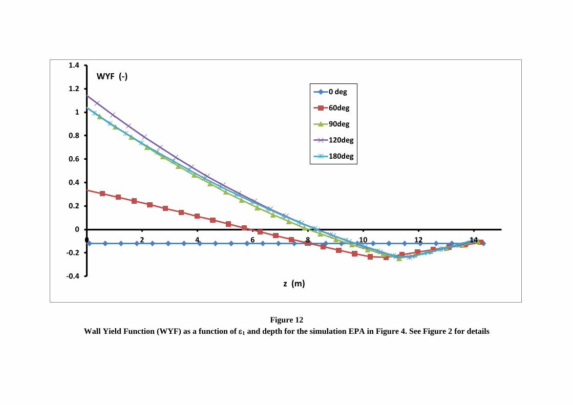
Figure 12
Wall Yield Function (WYF) as a function of 1 and depth for the simulation EPA in Figure 4. See Figure 2 for details
-0.4
-0.2
0
0.2
0.4
0.6
0.8
1
1.2
1.4
0 2 4 6 8 10 12 14
WYF (-)
z (m)
0 deg
60deg
90deg
120deg
180deg

Figure 13
Wall Yield Function (WYF) as a function of 1 and depth for the simulation of revised conditions for the ECA simulation. Conditions as
in Figure 4, Table 2 and Figure 12, except: w=7o; c=core=3.5
o
-0.3
-0.25
-0.2
-0.15
-0.1
-0.05
0
0 2 4 6 8 10 12 14
WYF (-)
z (m)
0 deg
60deg
90deg
120deg
180deg

Figure 14
CYF' for the principal stress cap at depth (Zo-Z) of 15m. Conditions as shown in Figure 13.
-2.0E+01
-1.5E+01
-1.0E+01
-5.0E+00
0.0E+00
5.0E+00
1.0E+01
1.5E+01
2.0E+01
2.5E+01
3.0E+01
1 (deg)
CYF'
X (m)

Figure 15
The Yield Quotient (YQ) for a range of simulations, including those in Figures 13 & 14. For details see Table 3.
0
0.1
0.2
0.3
0.4
0.5
0.6
0.7
0 5 10 15 20 25
YQ
depth (Zo-Z) (m)
basecase 1 Ecc=0.667
Ecc=0
Ecc=0.333
Ecc=0.5
Ecc=0.725
Ecc=0.8
Bw=3.5; Bc=1.75; Ecc=0.667
concave-1 Ecc=0
concave 2 Ecc=0

Figure 16 Wall stresses for a silo at incipient core-flow. For conditions see Table 4
Figure 16a wall normal stress versus z
0.0E+00
2.0E+04
4.0E+04
6.0E+04
8.0E+04
1.0E+05
1.2E+05
0 1 2 3 4 5 6 7 8 9 10
Wall normal stress
IF1; 0 deg
IF1; 90 deg
IF1; 180 deg
IF2; 0 deg
IF2; 90 deg
IF2; 180 deg

Figure 16 Wall stresses for a silo at incipient core-flow. For conditions see Table 4
Figure 16b wall vertical shear stress versus z
-1.0E+04
-8.0E+03
-6.0E+03
-4.0E+03
-2.0E+03
0.0E+00
2.0E+03
4.0E+03
6.0E+03
8.0E+03
0 1 2 3 4 5 6 7 8 9 10
Wall vertical shear stress
IF1; 0 deg
IF1; 90 deg
IF1; 180 deg
IF2; 0 deg
IF2; 90 deg
IF2; 180 deg

Figure 17 Switch stresses in a silo section 3m radius and 30m tall: conditions shown in Table 5
Figure 17a Principal stress 1 versus Cartesian coordinate z
0.0E+00
2.0E+04
4.0E+04
6.0E+04
8.0E+04
1.0E+05
1.2E+05
1.4E+05
0.00E+00 5.00E+00 1.00E+01 1.50E+01 2.00E+01 2.50E+01 3.00E+01
1 (Pa)
z (m)
0 deg
60 deg
90 deg
120 deg
180 deg

Figure 17 Switch stresses in a silo section 3m radius and 30m tall: conditions shown in Table 5
Figure 17b Principal stress 2 versus Cartesian coordinate z
0.0E+00
5.0E+04
1.0E+05
1.5E+05
2.0E+05
2.5E+05
3.0E+05
3.5E+05
4.0E+05
0.00E+00 5.00E+00 1.00E+01 1.50E+01 2.00E+01 2.50E+01 3.00E+01
2 (Pa)
z (m)
0 deg
60 deg
90 deg
120 deg
180 deg

Figure 17 Switch stresses in a silo section 3m radius and 30m tall: conditions shown in Table 5
Figure 17c Principal stress 3 versus Cartesian coordinate z
0.0E+00
1.0E+05
2.0E+05
3.0E+05
4.0E+05
5.0E+05
6.0E+05
0 5 10 15 20 25 30
3 Pa
z (m)
0 deg
60 deg
90 deg
120 deg
180 deg
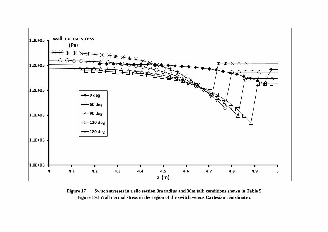
Figure 17 Switch stresses in a silo section 3m radius and 30m tall: conditions shown in Table 5
Figure 17d Wall normal stress in the region of the switch versus Cartesian coordinate z
1.0E+05
1.1E+05
1.1E+05
1.2E+05
1.2E+05
1.3E+05
4 4.1 4.2 4.3 4.4 4.5 4.6 4.7 4.8 4.9 5
wall normal stress (Pa)
z (m)
0 deg
60 deg
90 deg
120 deg
180 deg

Figure 18 Switch stresses in a silo section 3m radius and 30m tall with an increase in Kw below the switch: conditions shown in
Table 5
Figure 18a Principal stress 1 versus Cartesian coordinate z
0.0E+00
2.0E+04
4.0E+04
6.0E+04
8.0E+04
1.0E+05
1.2E+05
1.4E+05
1.6E+05
0 5 10 15 20 25 30
1 (Pa)
z (m)
0 deg
60 deg
90 deg
120 deg
180 deg

Figure 18 Switch stresses in a silo section 3m radius and 30m tall with an increase in Kw below the switch: conditions shown in
Table 5
Figure 18b Principal stress 2 versus Cartesian coordinate z
0.0E+00
5.0E+04
1.0E+05
1.5E+05
2.0E+05
2.5E+05
3.0E+05
3.5E+05
4.0E+05
4.5E+05
5.0E+05
0 5 10 15 20 25 30
2 (Pa)
z (m)
0 deg
60 deg
90 deg
120 deg
180 deg

Figure 18 Switch stresses in a silo section 3m radius and 30m tall with an increase in Kw below the switch: conditions shown in
Table 5
Figure 18c Principal stress 3 versus Cartesian coordinate z
0.0E+00
1.0E+05
2.0E+05
3.0E+05
4.0E+05
5.0E+05
6.0E+05
0 5 10 15 20 25 30
3 (Pa)
Zc m
0 deg
60 deg
90 deg
120 deg
180 deg

Figure 18 Switch stresses in a silo section 3m radius and 30m tall with an increase in Kw below the switch: conditions shown in
Table 5
Figure 18d Wall normal stress in the region of the switch versus Cartesian coordinate z
7.0E+04
8.0E+04
9.0E+04
1.0E+05
1.1E+05
1.2E+05
1.3E+05
1.4E+05
1.5E+05
4 4.2 4.4 4.6 4.8 5 5.2
wall normal stress (pa)
z (m)
0 deg
60 deg
90 deg
120 deg
180 deg

Figure 19 Wall normal stress for conditions close to those of maximum magnitude switch stress. For conditions see Table 5
Figure 19a Overall wall normal stress variation with depth with 1 (deg) as a parameter
0.0E+00
2.0E+04
4.0E+04
6.0E+04
8.0E+04
1.0E+05
1.2E+05
1.4E+05
1.6E+05
1.8E+05
0 5 10 15 20 25 30
wall normal stress (Pa)
z (m)
0 deg
60 deg
90 deg
120 deg
180 deg

Figure 19 Wall normal stress for conditions close to those of maximum magnitude switch stress. For conditions see Table 5
Figure 19b Wall normal stress in the region of the switch with 1 (deg) as a parameter
0.0E+00
2.0E+04
4.0E+04
6.0E+04
8.0E+04
1.0E+05
1.2E+05
1.4E+05
1.6E+05
1.8E+05
4 4.1 4.2 4.3 4.4 4.5 4.6 4.7 4.8 4.9 5
wall normal stress (Pa)
z (m)
0 deg
60 deg
90 deg
120 deg
180 deg

Figure 20 Wall stress measurements - relation to the state of stress, both at the wall
and internally
max
c min
c
Mohr Circle 1
Mohr Circle 2


