A primer to numerical simulations: The perihelion motion ... · A primer to numerical simulations:...

A primer to numerical simulations: The perihelionmotion of Mercury

C. Körber1, I. Hammer1, J.-L. Wynen1, J. Heuer2‡, C. Müller3

and C. Hanhart1

1 Institut für Kernphysik (IKP-3) and Institute for Advanced Simulations (IAS-4),Forschungszentrum Jülich, D-52425 Jülich, Germany2 Hochschule Hamm-Lippstadt, Marker Allee 76-78, 59063 Hamm, Germany3 Schülerlabor JuLab, Forschungszentrum Jülich, D-52425 Jülich, Germany

E-mail: [email protected], [email protected]

Abstract. Numerical simulations are playing an increasingly important role inmodern science. In this work it is suggested to use a numerical study of the famousperihelion motion of the planet Mercury (one of the prime observables supportingEinsteins General Relativity) as a test case to teach numerical simulations to highschool students. The paper includes details about the development of the code as wellas a discussion of the visualization of the results. In addition a method is discussed thatallows one to estimate the size of the effect as well as the uncertainty of the approacha priori. At the same time this enables the students to double check the results foundnumerically. The course is structured into a basic block and two further refinementswhich aim at more advanced students.

1. Introduction

Numerical simulations play a key role in modern physics because they allow one totackle some theoretical problems not accessible otherwise. This might be the casebecause there are too many particles participating in the system (as in simulationsfor weather predictions) or the interactions are too complicated to allow for asystematic, perturbative approach (as in theoretical descriptions of nuclear particles atthe fundamental level). This paper introduces a project that allows one to demonstratethe power of numerical simulations. On the example of the perihelion motion of theplanet Mercury the students are supposed to learn about

• the importance of differential equations in theoretical physics;

• the numerical implementation of Newtonian dynamics;

• systematic tests and optimization of computer codes;

‡ Present Address: Institut für Neurowissenschaften und Medizin (INM-4), Forschungszentrum Jülich,D-52425 Jülich, Germany

arX

iv:1

803.

0167

8v1

[ph

ysic

s.ed

-ph]

5 M

ar 2

018

A primer to numerical simulations 2

• effective tools to estimate the result a priori as an important cross check;

• the visualization of numerical results using VPython.

We are convinced that in order to excite students for numerical simulations it iscompulsory to demonstrate their power on an example that catches their interest.This purpose is served perfectly by the case chosen here, since Einsteins equationsof General Relativity are fascinating to a very broad public. Their detailed studyneeds a deep understanding of Differential Geometry. For the course presented here,however, very little math is necessary, such that high school students vaguely familiarto vector calculus and derivatives will benefit from it. This was already demonstrated inthe “Schülerakademie Teilchenphysik”, where this course was tested successfully on twogroups consisting in total of 24 German high school students from 10th to 13th grade in2015 and 2017.

The course as well as this paper is structured as follows: after an introductionto Newtonian dynamics and the concept of differential equations, their discretizationis discussed based on Newton’s law of gravitation and possible extensions thereof.Afterwards the visualization of the resulting trajectories using VPython is introducedand applied to the problem at hand. In addition, tools are developed to extract therelevant quantity from the result of the simulation. Finally, the principle of dimensionalanalysis is presented as a tool to estimate the size of the effect studied as well as itsexpected accuracy. Furthermore the method allows one to cross check the results of thesimulation. As is pointed out in the chapters below the course can be finished at somecanonical points — in particular we think that for most students a detailed study of theuncertainties of the numerical simulations might be too technical. However, we includethis discussion as well both for completeness and as an additional challenge to the moreadvanced students.

2. Trajectories, velocities, accelerations and Newton’s second law

A physical system is said to be understood, if the assumed forces acting on it lead to theobserved trajectories. In other words, we need to show that we can calculate the locationin space of the object of interest at any future point in time, once the initial conditionsare fixed properly. If we can neglect the finite size of this object (and in particularits orientation in space), the location is parametrized by a single three vector ~r(t).Additionally, we need to be able to calculate the objects velocity ~v(t) and acceleration~a(t) in order to describe and control its dynamics; this will become clear below. Thevelocity describes a change of location over time which, for some infinitesimally small∆t, can be written as

~r(t+ ∆t) = ~r(t) + ~v(t)∆t+ . . . . (1)

Similarly, the acceleration describes a change in velocity, i.e.

~v(t+ ∆t) = ~v(t) + ~a(t)∆t+ . . . . (2)


The dots in these expressions indicate additional terms that may be expressed in termsof higher powers in ∆t. While they are needed in general, for sufficiently small ∆t theycan be safely neglected. Thus we may define the time derivative via

~v(t) = lim∆t→0

∆~r(t)

∆t=:

d~r(t)

dt= ~r(t) , (3)

where ∆~r(t) = ~r(t + ∆t) − ~r(t) and we introduced a common short hand notation fortime derivatives in the last expression. Analogously we get

~a(t) = lim∆t→0

∆~v(t)

∆t=:

d~v(t)

dt= ~v(t) , (4)

=d2~r(t)

dt2= ~r(t) , (5)

where we introduced the second derivative in the second line.It was Newton who observed that, if a body is at rest, it will remain at rest, and if it

is in motion it will remain in motion at a constant velocity in a straight line, unless it isacted upon by some force — this is known as Newton’s first law. Formulated differently:a force ~F expresses itself by changing the motion of some object. This is quantified inNewton’s second law

~F (~r, t) =d

dt(m~v) . (6)

If the mass does not change § with time, this reduces to the well known

~F (~r) = m~a(t) = m~v(t) = m~r(t) . (7)

Note that in general the force could depend also on the time or the velocity. Here,we restrict ourselves to the case relevant for our example, where the force depends onthe location only. Therefore, as soon as the force ~F (~r) is known for all ~r one can inprinciple calculate the trajectory by solving Eq. (7) for ~r(t). Sometimes this requiressome advanced knowledge of mathematics and sometimes no closed form solution exists.However, alternatively one can calculate the whole trajectory of some test body thatexperiences this force by a successive application of the rules given in Eqs. (1) and (2):

(i) For a given time t, where ~r(t) and ~v(t) are known, use the force to calculate~a(t) = ~F (~r(t))/m, see Eq. (7).

(ii) Use Eq. (1) to calculate ~r(t+ ∆t).

(iii) Use Eq. (2) to calculate ~v(t+ ∆t).

(iv) Go back to (i) with t→ t+ ∆t.

Clearly to initiate the procedure at some time t0 both ~r(t0) as well as ~v(t0) must beknown — the trajectories depend on these initial conditions ‖.§ A well known example where m does change with time is a rocket, whose mass decreases as fuel isburned.‖ In general, a differential equation of nth degree (where the highest derivative is order n) needs n

initial conditions specified. For n = 2 those are often chosen as location and velocity at some startingtime, but one may as well pick two locations at different times.


This procedure can only work if ∆t is sufficiently small. One way to estimatewhether ∆t is small enough is to verify whether the relation

|~v(t)| � 1

2|~a(t)|∆t =

1

2m|~F (~r(t))|∆t (8)

holds. This follows from Eq. (1) where the first term that we neglected reads(1/2)a(t)(∆t)2. Eq. (8) also shows that small (large) time steps are necessary (sufficient),if the force is strong (weak), since the time steps need to be small enough that all changesinduced by the force get resolved. Clearly, a relation as Eq. (8) can only provide guidanceand can not replace a careful numerical check of the solutions: A valid result has to beinsensitive to the concrete value chosen for ∆t — in particular replacing ∆t by ∆t/2

should not change the result significantly. This issue will be discussed in more detailbelow.

3. Example: General Relativity and the perihelion motion of Mercury

For this concrete example the starting point for the force is Newton’s law of gravitation

~FN(~r) = −GNmM�r2

~r

r, (9)

where GN = 6.67 × 10−11 m3kg−1s−2 is the Newtonian constant of gravitation, m isthe mass of Mercury and M� = 1.99 × 1030 kg is the mass of the Sun. In additionr = |~r(t)| denotes the distance between Sun and Mercury, when we assume that the Sunis infinitely heavier than Mercury and located at the center of the coordinate system.Although this is not exact, it is a good approximation because m/M� ∼ 10−8. For laterconvenience we introduce the Schwarzschild radius of the Sun

rS =2GNM�

c2= 2.95 km , (10)

where c = 3.00× 108 m/s denotes the speed of light. Note that rS is the characteristiclength scale of the gravitational field of the Sun for — up to the prefactor — onecan not form another quantity with dimensions of a length from GN , M� and c. TheSchwarzschild radius is also an important quantity to characterize black holes; this ishowever not relevant for the discussion at hand. With this, Newton’s second law reads

~r = −c2

2

(rSr2

) ~rr. (11)

An attractive force that vanishes at large distances leads in general, depending on theinitial conditions, either to bounded or to open orbits. In the latter case the planetsimply disappears from the Sun, since a given force can capture only bodies with smallenough momenta. The students may study those scenarios within their simulations byvarying the start velocity while keeping the start location fixed.

The bounded orbits that emerge from a potential that scales as 1/r (whichcorresponds to a force that scales as 1/r2) are elliptic and fixed in space. In particularthe point of closest approach of the planet to the Sun, the perihelion, does not move.However, when a potential that vanishes for r → ∞ deviates from 1/r, the perihelion


does move. This makes the behavior of the perihelion a very sensitive probe of thegravitational potential.

The observed perihelion motion of Mercury is nowadays determined as

(574.10± 0.65)′′ per 100 earth years [1]

where the symbol ′′ denotes “arc seconds”: 1′′ = (1/3600)o. The bulk of this numbercan be understood by the presence of other planets within the Newtonian theory, sincetheir gravitational force also acts on Mercury. However, a residual motion of

δΘM = (42.56± 0.94)′′ per 100 earth years [1] (12)

remained unexplained, until Einstein quantified the predictions of General Relativity tothis particular observable [2]

δΘGR = (43.03± 0.03)′′ per 100 earth years [1] . (13)

To allow for a movement of the perihelion we need to modify the force that ledto Eq. (11). This modification should be such that it depends on r and it vanishes forr →∞. Based on the discussion presented above we may multiply the right hand sideof (11) with a factor (1 + α rS

r), where α denotes some dimensionless parameter. This

seems like a natural way to parametrize the additional potential because it adds thesmallest possible deviation from a 1/r potential expressed relative to the characteristiclength rS. However, besides rS, which characterizes the gravitational potential of theSun, there is also a characteristic parameter for the dynamics of Mercury:

r2L :=

~L 2

m2c2=

(~r × ~r )2

c2, (14)

where ~L denotes the angular momentum, which is a constant of motion for centralpotentials. It is easily verified that r2

L carries dimensions of length squared. We thereforehave to add one more term to the potential; in analogy to the one discussed above, weuse β r2L

r2. Here one might wonder why this additional term is chosen proportional to

(rL/r)2 and not to (rL/r). The reason for this choice is indeed not obvious: In general

the correction terms added must be scalar quantities — accordingly vectors can enteronly as scalar products. Moreover, one is not allowed to use square-roots of those scalarproducts for these impose wrong mathematical properties to the equations of motion(for the case at hand, e.g., the derivative with respect to the velocity would not bedefined at ~r = 0) — the only vector that is allowed to appear as its length in linearorder is the radius, since this length is related to geometrical properties of the system.Combining everything, we use the following ansatz for the modified equation of motion:

~r = −c2

2

rSr2

(1 + α

rSr

+ βr2L

r2

)~r

r. (15)

For the system at hand, r2L may be estimated from the parameters of Mercury at its

perihelion: The corresponding velocity is r(t = 0) = |~vM(0)| = 59.0 km/s (here wealready indicate that we will start the simulation at the perihelion) and the closestdistance between Sun and Mercury is rMS = |~rMS(0)| = 46.0 · 106 km [3]. Note that


at the perihelion ~r and ~r are perpendicular to each other (see Figure 1). We thus findthat (r2

L/r2MS) ∼ 4 · 10−8. Furthermore (rS/rMS) ∼ 6 · 10−8. Therefore one may expect

from both correction terms an effect of similar size — for a more detailed discussionabout the underlying logic we refer to Sec. 6. Furthermore, any term of higher order ineither r2

L or rS should be suppressed by additional seven orders of magnitude and thuscan be neglected safely. The parameters α and β can be extracted from a fit to data.However, since we have only a single number to study, the perihelion shift (see Eq. (12)),we can only fix either α or β (or a linear combination thereof). The parameters canalso be calculated from the underlying theory one uses. The actual values depend onthe specific theory; General Relativity gives [2]

α = 0 , β = 3 . (16)

Thus we may also use the simulation explained below to calculate the perihelion motionof Mercury from the input values given in Eq. (16). Modifications to the Newtonianequation of gravity introduced to account for the perihelion motion of Mercury arediscussed in great detail in a very pedagogical way also in Ref. [4].

4. Numerical Implementation

4.1. Describing the Motion with Python

In this section we present the numerical implementation as well as the visualizationof planetary trajectories and in particular the perihelion motion of Mercury. Wechoose Python [5] as programming language because Python is easy to learn, intuitiveto understand and an open source language. No prior knowledge of Python or anyother programming language is required, as we explain all necessary steps to createthe simulation. In the following, we present code examples which tested for Pythonversion 3.6.4 and VPython version 7.3.2. We provide online instructions for settingup Python and VPython on different operating systems [6]. In Appendix A, we alsoprovide a working example as well as possible extensions and template files online.

To start the simulation one needs the “initial” distance and velocity [Eq. (1) andEq. (2)]. As described above, here one can simplify the problem by placing one object(the “infinitely” heavy Sun) in the center of the coordinate system and keep it fixed.

Since the trajectories do not depend on where on the orbit of Mercury the simulationis started, we use the values at the perihelion with |~rMS(0)| = 46.0 · 106 km and|~vM(0)| = 59.0 km/s [3] as initial (for t = 0) parameters. The computer does notunderstand physical units, hence one has to express each variable in an appropriateunit. Both for the numerical treatment and the intuitive understanding, it is useful toselect parameters in a “natural range”, e.g., by expressing distances in R0 = 1010 m andtime intervals in days, T0 = 1 d, where d refers to earth days. One Mercury year is givenby TM = 88.0T0. With this choice, the initial distance of Mercury to the Sun, the size


of the initial velocity of Mercury and the acceleration prefactor (see Eq. (15)) become

rMS(0) = 4.60R0 , vM(0) = 0.510R0

T0

, (17)

aMS(rMS) =c2

2

rSr2MS

= 0.990R0

T 20

1

(rMS/R0)2 . (18)


# Update v e l o c i t y vec to r

vec vM new = vec vM old + vec aMS ∗ dt

# Update po s i t i o n vec to r

vec rM new = vec rM old + vec vM new ∗ dt

Note the beauty of working with the predefined vector class: the basic vector operations

are already implemented. The difference and sum of two vectors, or the scalar vector

multiplication return vectors themselves. Also the magnitude of a vector – vector.mag

– is a property of the vector and can be easily extracted.

It is handy to use Pythons functions to embed repeating structures (”DRY” –

Don’t Repeat Yourself)

# Def ine the func t i on

de f evo lve mercury ( vec rM old , vec vM old ) :

< . . . Code . . . >

re turn vec rM new , vec vM new

# Cal l the func t i on

vec rM new , vec vM new = do t ime s t ep ( vec rM old , vec vM old )

Because of Python s syntax, it is necessary that the body of the function is indented

relative to the definition statement.

Finally, we can express the evolution by a while-loop

t = 0

# Execute the loop as long as t < T

whi le t < T:

vec rM , vec vM = evolve mercury ( vec rM , vec vM)

t = t + dt

Note the required indent of the loop structure similar to the indent of a function. In

each iteration of the while-loop, the previous distance and velocity are used to compute

the new values – which directly overwrite the previous values and thus enter the next

iteration. The time step dt needs to be sufficiently small in order to avoid numerical

errors. We recommend dt = .... The total runtime T is the amount of ”virtual” days the

simulations should run. To describe at least one full orbit, T needs to be larger than

T > ...

Ideas for questions:

• Mass and motion of sun

• Estimate dt and also T in order to cover roughly two ”mercury years”.

• What does happen when you change those units?

• Compare values to the values in []. Where does the difference come from?

• Start with α = 0. What do you observe?

rM vM aMS


# Update v e l o c i t y vec to r

vec vM new = vec vM old + vec aMS ∗ dt

# Update po s i t i o n vec to r

vec rM new = vec rM old + vec vM new ∗ dt

Note the beauty of working with the predefined vector class: the basic vector operations

are already implemented. The difference and sum of two vectors, or the scalar vector

multiplication return vectors themselves. Also the magnitude of a vector – vector.mag

– is a property of the vector and can be easily extracted.

It is handy to use Pythons functions to embed repeating structures (”DRY” –

Don’t Repeat Yourself)

# Def ine the func t i on

de f evo lve mercury ( vec rM old , vec vM old ) :

< . . . Code . . . >

re turn vec rM new , vec vM new

# Cal l the func t i on

vec rM new , vec vM new = do t ime s t ep ( vec rM old , vec vM old )

Because of Python s syntax, it is necessary that the body of the function is indented

relative to the definition statement.

Finally, we can express the evolution by a while-loop

t = 0

# Execute the loop as long as t < T

whi le t < T:

vec rM , vec vM = evolve mercury ( vec rM , vec vM)

t = t + dt

Note the required indent of the loop structure similar to the indent of a function. In

each iteration of the while-loop, the previous distance and velocity are used to compute

the new values – which directly overwrite the previous values and thus enter the next

iteration. The time step dt needs to be sufficiently small in order to avoid numerical

errors. We recommend dt = .... The total runtime T is the amount of ”virtual” days the

simulations should run. To describe at least one full orbit, T needs to be larger than

T > ...

Ideas for questions:

• Mass and motion of sun

• Estimate dt and also T in order to cover roughly two ”mercury years”.

• What does happen when you change those units?

• Compare values to the values in []. Where does the difference come from?

• Start with α = 0. What do you observe?

rM vM aMS

x y

z~rMS

Figure 1: Sun-Mercury system with relevant vectors. Mercury is at its perihelion,therefore its velocity is perpendicular to its direct connection vector with the sun.

In Python, this reads# Definition of parametersrM0 = 4.60 # Initial radius of Mercury orbit, in units of R0vM0 = 5.10e-1 # Initial orbital speed of Mercury, in units of R0/T0c_a = 9.90e-1 # Base acceleration of Mercury, in units of R0**3/T0**2TM = 8.80e+1 # Orbit period of MercuryrS = 2.95e-7 # Schwarzschild radius of Sun,in units of R0rL2 = 8.19e-7 # Specific angular momentum, in units of R0**2

where c_a = aMSr2MS, the acceleration without the radius factor. The last two quantities

refer to the Schwarzschild radius of the Sun and the parameter r2L defined in Eqs. (10)

and (14), respectively.So far we only fixed the length of the vectors. Next, we set up the initial

directions, which will describe the motion in space. We will build on the existing Pythonmodule VPython, which provides an implementation for treating vectors as well as theirvisualization. The first object of interest is a vector, which takes three-dimensionalcoordinates as its input. With our choice of initial conditions (we picked the initialvectors in the perihelion), the velocity of Mercury is perpendicular to the vector whichconnects Mercury and Sun (see figure 1):# Import the class vector from vpythonfrom vpython import vector# Initialize distance and velocity vectorsvec_rM0 = vector(0, rM0, 0)vec_vM0 = vector(vM0, 0, 0)


¶ We use the estimate of Eq. (8) as a guidance to fix the time step ∆t as

# Definition of the time stepdt = 2 * vM0 / c_a / 20

Here the factor 1/20 makes sure that ∆t is indeed consistent with Eq. (8). Now weare in the position to calculate location and velocity of the planet at t0 + ∆t using thefollowing expressions+

# Compute the strength of the accelerationtemp = 1 + alpha * rS / vec_rM_old.mag + beta * rL2 / vec_rM_old.mag**2aMS = c_a * temp / vec_rM_old.mag**2# Multiply by the directionvec_aMS = - aMS * ( vec_rM_old / vec_rM_old.mag )# Update velocity vectorvec_vM_new = vec_vM_old + vec_aMS * dt# Update position vectorvec_rM_new = vec_rM_old + vec_vM_new * dt

Note basic vector operations are already implemented in the predefined vector class.The difference and sum of two vectors, or the scalar vector multiplication return vectorsthemselves. Also the magnitude of a vector — vector.mag — is an attribute of the vectorand can be easily extracted.

It is handy to use Pythons functions to structure the program and hold repeatingcode (“DRY” — Don’t Repeat Yourself):

# Define the coordinate and velocity update functiondef evolve_mercury(vec_rM_old, vec_vM_old, alpha, beta): # Compute the strength of the acceleration temp = 1 + alpha * rS / vec_rM_old.mag + beta * rL2 / vec_rM_old.mag**2 aMS = c_a * temp / vec_rM_old.mag**2 # Multiply by the direction vec_aMS = - aMS * ( vec_rM_old / vec_rM_old.mag ) # Update velocity vector vec_vM_new = vec_vM_old + vec_aMS * dt # Update position vector vec_rM_new = vec_rM_old + vec_vM_new * dt return vec_rM_new, vec_vM_new

# Call the functionvec_rM_new, vec_vM_new = evolve_Mercury(vec_rM_old, vec_vM_old, 0.0, 0.0)

Pythons syntax enforces a clean programming style: it is necessary that the body of the

¶ Note that the code is designed for VPython versions 7 and later. For VPython versions prior 7, e.g.,the statement from vpython import vector must be replaced by from visual import vector .+ Note, that there are different notions for numerically integrating differential equations with differentaccuracies. Thus, the ordering and exact expressions for updating aMS , vM and rMS are not unique.However, all correct prescriptions lead to the same result for sufficiently small ∆t. For this particularproblem, the definitions we show are in good balance between being numerically stable and inexpensiveto compute.


function is indented (by an arbitrary but consistent amount of spaces∗) relative to thedefinition statement of the function. Furthermore, Python is an Interpreter language.Each line of the code is executed when the Interpreter passes it. For this reason, ifwe define the parameters before the function, they can be used inside of the function.Variables defined within the function (e.g. aMS , vec_aMS , . . .) are local and do not existbeyond the scope of the function; they can not be used after the return statement.

Finally, we can describe the evolution by a while-loop

t = 0.0alpha = 0.0beta = 0.0# Set position and velocity to their starting pointsvec_rM = vec_rM0vec_vM = vec_vM0# Execute the loop as long as t < 2*TMwhile t < 2*TM: # Update position and velocity vec_rM, vec_vM = evolve_mercury(vec_rM, vec_vM, alpha, beta) # Advance time by one step t = t + dt

where for the start we set the parameters α = 0 = β in order to first study the propertiesof the pure 1/r2 force. Note the required indent of the loop structure similar to the indentof a function. In each iteration of the while-loop, the previous distance and velocityare used to compute the new values, directly overwriting the previous values. The totalruntime 2*TM is the amount of “virtual” days the simulations should run. To describeat least one full orbital period, this time needs to be larger than TM . With the previouschoice for dt, this corresponds to roughly NT ≈ 2 · 103 evolution steps. Note that theexact time it takes for Mercury to complete a full revolution depends on the initialcoordinates and velocities, the accuracy of the computation (controlled by the value of∆t) as well as the computing power employed. One should encourage the students toanalyze this in the beginning.

4.2. Visualizing the Motion with VPython

To start the visualization one has to import further objects from the VPython module.We change the import statement from before to

from vpython import vector, sphere, color, curve, rate

The class sphere will represent Mercury and the Sun in the simulation

# Define the initial coordinates; M = Mercury, S = SunM = sphere(pos=vec_rM0, radius=0.5, color=color.red )S = sphere(pos=vector(0,0,0), radius=1.5, color=color.yellow)# And the initial velocities

∗ While Python allows using tabs as well, this can cause programming errors, because their displayedwidth depends on the text editor.


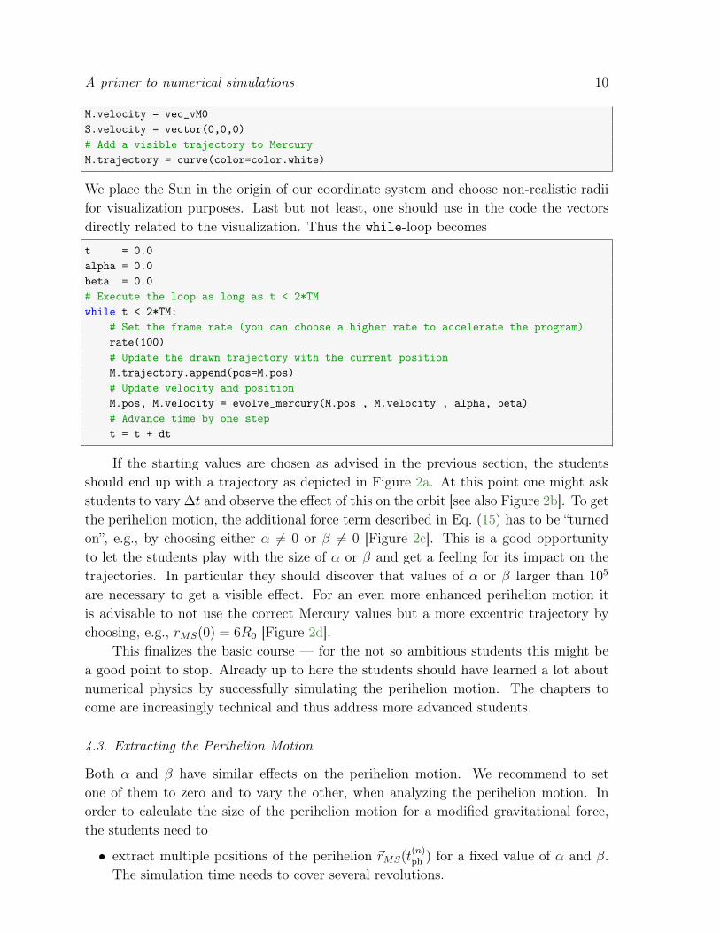
M.velocity = vec_vM0S.velocity = vector(0,0,0)# Add a visible trajectory to MercuryM.trajectory = curve(color=color.white)

We place the Sun in the origin of our coordinate system and choose non-realistic radiifor visualization purposes. Last but not least, one should use in the code the vectorsdirectly related to the visualization. Thus the while-loop becomes

t = 0.0alpha = 0.0beta = 0.0# Execute the loop as long as t < 2*TMwhile t < 2*TM: # Set the frame rate (you can choose a higher rate to accelerate the program) rate(100) # Update the drawn trajectory with the current position M.trajectory.append(pos=M.pos) # Update velocity and position M.pos, M.velocity = evolve_mercury(M.pos , M.velocity , alpha, beta) # Advance time by one step t = t + dt

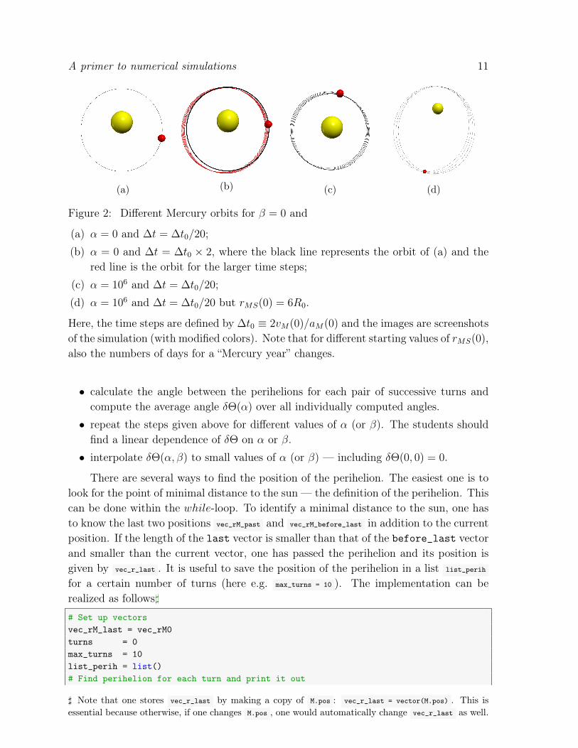
If the starting values are chosen as advised in the previous section, the studentsshould end up with a trajectory as depicted in Figure 2a. At this point one might askstudents to vary ∆t and observe the effect of this on the orbit [see also Figure 2b]. To getthe perihelion motion, the additional force term described in Eq. (15) has to be “turnedon”, e.g., by choosing either α 6= 0 or β 6= 0 [Figure 2c]. This is a good opportunityto let the students play with the size of α or β and get a feeling for its impact on thetrajectories. In particular they should discover that values of α or β larger than 105

are necessary to get a visible effect. For an even more enhanced perihelion motion itis advisable to not use the correct Mercury values but a more excentric trajectory bychoosing, e.g., rMS(0) = 6R0 [Figure 2d].

This finalizes the basic course — for the not so ambitious students this might bea good point to stop. Already up to here the students should have learned a lot aboutnumerical physics by successfully simulating the perihelion motion. The chapters tocome are increasingly technical and thus address more advanced students.

4.3. Extracting the Perihelion Motion

Both α and β have similar effects on the perihelion motion. We recommend to setone of them to zero and to vary the other, when analyzing the perihelion motion. Inorder to calculate the size of the perihelion motion for a modified gravitational force,the students need to

• extract multiple positions of the perihelion ~rMS(t(n)ph ) for a fixed value of α and β.

The simulation time needs to cover several revolutions.


(a) (b) (c) (d)

Figure 2: Different Mercury orbits for β = 0 and

(a) α = 0 and ∆t = ∆t0/20;

(b) α = 0 and ∆t = ∆t0 × 2, where the black line represents the orbit of (a) and thered line is the orbit for the larger time steps;

(c) α = 106 and ∆t = ∆t0/20;

(d) α = 106 and ∆t = ∆t0/20 but rMS(0) = 6R0.

Here, the time steps are defined by ∆t0 ≡ 2vM(0)/aM(0) and the images are screenshotsof the simulation (with modified colors). Note that for different starting values of rMS(0),also the numbers of days for a “Mercury year” changes.

• calculate the angle between the perihelions for each pair of successive turns andcompute the average angle δΘ(α) over all individually computed angles.

• repeat the steps given above for different values of α (or β). The students shouldfind a linear dependence of δΘ on α or β.

• interpolate δΘ(α, β) to small values of α (or β) — including δΘ(0, 0) = 0.

There are several ways to find the position of the perihelion. The easiest one is tolook for the point of minimal distance to the sun — the definition of the perihelion. Thiscan be done within the while-loop. To identify a minimal distance to the sun, one hasto know the last two positions vec_rM_past and vec_rM_before_last in addition to the currentposition. If the length of the last vector is smaller than that of the before_last vectorand smaller than the current vector, one has passed the perihelion and its position isgiven by vec_r_last . It is useful to save the position of the perihelion in a list list_perih

for a certain number of turns (here e.g. max_turns = 10 ). The implementation can berealized as follows]

# Set up vectorsvec_rM_last = vec_rM0turns = 0max_turns = 10list_perih = list()# Find perihelion for each turn and print it out

] Note that one stores vec_r_last by making a copy of M.pos : vec_r_last = vector(M.pos) . This isessential because otherwise, if one changes M.pos , one would automatically change vec_r_last as well.


while turns < max_turns: vec_rM_before_last = vec_rM_last # Store position of Mercury in a new vector (since we will change M.pos) vec_rM_last = vector(M.pos) #<...update Mercury position...> # Check if at perihelion if (vec_rM_last.mag < M.pos.mag) and (vec_rM_last.mag < vec_rM_before_last.mag): list_perih.append(vec_rM_last) turns = turns + 1

The angle between two vectors can be computed using

^(~v1, ~v2) = arccos

(~v1 · ~v2

|~v1| |~v2|

). (19)

This is readily implemented in VPython via

# Import functions to compute anglefrom vpython import acos, pi, dot# Define function for angle extractiondef angle_between(v1, v2): return acos( dot(v1, v2) / (v1.mag * v2.mag) ) * 180. / pi

where the factor 180/π in the last line converts the unit of the angle from radians intodegrees. To account for the statistical errors (e.g. numerical rounding errors) one canaverage over a few turns. Depending on the programming proficiency of the studentsand time constraints, this can be done either by hand or, e.g., by implementing thefollowing code

sum_angle=0.for n in range(1, max_turns): # Calculate angle sum_angle = sum_angle + angle_between(list_perih[n-1], list_perih[n])# Display the averageprint(sum_angle/(max_turns-1))

Note that the perihelion motion is computed from the locations stored in list_perih andnot based on the initial position. This is important because depending on the initialconditions and numerical uncertainties, the simulation does not necessarily start in theexact perihelion.

As explained above [and further discussed in Section 6] the natural value for α (andβ) would be of the order of 1. However, if the students use this value for α, they will findthat the change in the trajectories is close to invisible and the numerical uncertainty ismuch larger than the result. It is therefore more advisable to use the fact that thereis a linear dependence between α and δΘ to estimate the size of the perihelion motion.On the other hand as soon as the values of α or β get too large the effective ansatz touse only the leading terms in the (rs/r) and (rL/r)

2 expansion is no longer justified andthe method of extraction might get unreliable. At this point we therefore recommendto choose the parameters α and β at most of the order of 105 — this value will be betterjustified in Section 6.


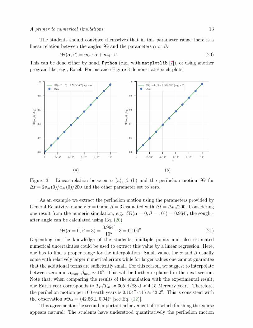
The students should convince themselves that in this parameter range there is alinear relation between the angles δΘ and the parameters α or β:

δΘ(α, β) = mα · α +mβ · β . (20)

This can be done either by hand, Python (e.g., with matplotlib [7]), or using anotherprogram like, e.g., Excel. For instance Figure 3 demonstrates such plots.

0 2 · 104 4 · 104 6 · 104 8 · 104 105

α

0.0

0.2

0.4

0.6

0.8

1.0

δΘ(α,β

) [de

g]

δΘ(α, β= 0) = 9.592 · 10−6[deg]×αData

(a)

0 2 · 104 4 · 104 6 · 104 8 · 104 105

β

0.0

0.2

0.4

0.6

0.8

1.0

δΘ(α,β

) [de

g]

δΘ(α= 0, β) = 9.643 · 10−6[deg]× βData

(b)

Figure 3: Linear relation between α (a), β (b) and the perihelion motion δΘ for∆t = 2vM(0)/aM(0)/200 and the other parameter set to zero.

As an example we extract the perihelion motion using the parameters provided byGeneral Relativity, namely α = 0 and β = 3 evaluated with ∆t = ∆t0/200. Consideringone result from the numeric simulation, e.g., δΘ(α = 0, β = 105) = 0.964°, the sought-after angle can be calculated using Eq. (20)

δΘ(α = 0, β = 3) =0.964°

105· 3 = 0.104′′ . (21)

Depending on the knowledge of the students, multiple points and also estimatednumerical uncertainties could be used to extract this value by a linear regression. Here,one has to find a proper range for the interpolation. Small values for α and β usuallycome with relatively larger numerical errors while for larger values one cannot guaranteethat the additional terms are sufficiently small. For this reason, we suggest to interpolatebetween zero and αmax, βmax ∼ 105. This will be further explained in the next section.Note that, when comparing the results of the simulation with the experimental result,one Earth year corresponds to TE/TM ≈ 365 d/88 d ≈ 4.15 Mercury years. Therefore,the perihelion motion per 100 earth years is 0.104′′ ·415 ≈ 43.2′′. This is consistent withthe observation δΘM = (42.56± 0.94)′′ [see Eq. (12)].

This agreement is the second important achievement after which finishing the courseappears natural: The students have understood quantitatively the perihelion motion


of Mercury. The next section that finalizes the numerical investigation is even moretechnical and should be worked on by the most advanced students only.

5. Tests of stability and error analysis

Measurements as well as numerical simulations in physics should always be accompaniedby estimates of the corresponding uncertainties. It is important for the students torecognize this fact and to understand what the sources of uncertainties are. The studentsshould therefore explore sources and sizes of inaccuracies arising in this simulation atleast qualitatively.

There are many potential sources of uncertainties in a simulation and discussing allof them is be beyond the scope of this work. Instead, we focus on the most accessiblesource: Numerical errors due to finite time steps ∆t. Additional sources of errors includethe omission of terms in Eqs. (1) and (2) and the infinite mass approximation of theSun (i.e. keeping the Sun’s position fixed).

Consider Figure 4, where the angle of the perihelion motion δΘ is shown for thefirst 10 turns (x-axis) for different choices of ∆t (colors) and β (columns). In all casesα = 0. As expected, δΘ is approximately constant for sufficiently small time-steps ∆t

and its value depends solely on β. However, contrary to the correct result δΘ deviatesfrom zero for α = 0 = β for all ∆t. Using the data points in Figure 3 and extrapolatingto α = 0 = β without enforcing δΘ(0, 0) = 0 leads to a similar offset. This offset is anumerical error and can be taken as an estimate for the error of the simulation.

0 2 4 6 8 10Nt

0.00

0.01

0.02

0.03

0.04

δΘ(α,β

) [de

g]

α= 0, β= 0

0 2 4 6 8 10Nt

0.5

0.6

0.7

0.8

0.9

1.0

1.1

α= 0, β= 1 · 105

0 2 4 6 8 10Nt

9.7

9.8

9.9

10.0

10.1

10.2

10.3

α= 0, β= 1 · 106

∆t0/∆t= 10

∆t0/∆t= 100

∆t0/∆t= 200

∆t0/∆t= 500

Figure 4: The motion of the perihelion δΘ in degrees depending on the number ofturns Nt for different time steps ∆t (color) and different values for β (columns). Here,∆t0 ≡ 2vM(0)/aM(0). Offsets of δΘ(α = 0, β = 0) from zero can be used as an estimateof the magnitude of the error. Oscillations in δΘ indicate too coarse time steps. Notethe change in scale for the different plots.

Furthermore, one can observe that for large time-steps the values of the perihelionmotion oscillate between discrete values at different turns. This can be explained as


follows: The sample code we present to find the perihelion vectors only finds theposition closest to the Sun amongst the discrete set of vectors evaluated at the discretizedtime steps and labels it as perihelion vector. However, this is only an approximation:Sometimes the program finds a point before and sometimes after the perihelion causingthe oscillations observed. The precision of this approximation improves as the time-step shrinks. Hence, strongly visible oscillations in δΘ for a different number of turnsindicate that the time-step used is too large.

This problem can be pointed out to the students by asking them to vary the size ofthe time-steps and observe the effect on the trajectories. This should also be done for awide range of values to show both good and problematic regimes. It is advantageous toset both α and β to zero for this study, since in this case the trajectories should be closedand deviations from the correct case can be spotted easily. Figure 2b shows the Mercurytrajectory for ∆t = 2vM(0)/aM(0)× 2. One can clearly see the failure of the simulationto reproduce the physical trajectory shown as the black, solid line. From examples likethis it should be apparent that the time steps influence the accuracy of the simulation.The simulation reproduces the actual trajectory only in the limit ∆t→ 0. Thus, in anynumerical simulation one always has to identify a proper compromise between numericalaccuracy and time spent for the simulation (clearly for ∆t→ 0 the computing time goesto infinity).

As a first estimate, one can approximate the numerical uncertainty of the perihelionmotion, ∆δΘ(α, β) at non-zero α and β, by its offset at α = 0 = β, the amplitude ofits oscillation at α = 0 = β as well as the amplitude of its oscillation at the non-zerovalues of α and β used for the actual calculation.

∆δΘ(α, β) =√δΘ2

mean(0, 0) + δΘ2std(0, 0) + δΘ2

std(α, β) , (22)

δΘmean(α, β) =1

Nt

Nt∑n=1

δΘn(α, β) , (23)

δΘ2std(α, β) =

1

Nt − 1

Nt∑n=1

[δΘmean(α, β)− δΘn(α, β)]2 , (24)

where the standard deviations and mean values are obtained from the data sample ofNt turns (orbits of mercury). Thus, the numerical value extracted is given by

δΘ(α, β) = δΘmean(α, β)±∆δΘ(α, β) . (25)

Note that this has to be repeated for each different time step ∆t.The absolute value of the numerical error mostly depends on the time step ∆t and

is roughly independent of the values of α and β. Therefore, it is more desirable to picklarge values for α and β, because this increases the absolute size of the perihelion motionand thus decreases the relative numerical error. However, there is a competing effectwhich places upper bounds on the values of α and β. For instance, the prediction forthe perihelion motion coming from General Relativity allowing for varying values of β


is given by

δΘGR(β) = 2π

[β

4

r2S

r2L

+O(β2 r

4S

r4L

)]. (26)

Thus, for large values of β, quadratic corrections in β become relevant and it is notpossible to extract the perihelion growth of Mercury by performing a linear interpolation.We display these competing effects in Figure 5. The relative difference betweennumerically extracted values and the General Relativity prediction for δΘ are plottedagainst β for zero α. The value of β we recommend for the extraction is of the order of 105

as will be further motivated in the next section. As can be seen in the figure: For smallervalues of β, the relative numerical uncertainty grows, while for larger values, β & 105,the numerical values deviate from the assumed linear dependence on β. Identifying aparameter space for reliable and precise computations is a general challenge for numericalsimulations.

104 105 106

β

20

15

10

5

0

5

10

15

20

δΘ(α

=0,β)−δΘ

GR(α

=0,β) i

n %

∆t0/∆t= 100

∆t0/∆t= 200

∆t0/∆t= 500

Figure 5: Difference of numerically extracted perihelion motion relative to the valuecomputed from General Relativity [Eq. (26)] for different time steps. The error bandsare computed according to Eq. (22).

6. Dimensional analysis

Dimensional analysis is not only a tool that allows one to cross check, if the resultsof simulations are of the right order of magnitude, it is also very helpful to identify


unusual dynamics in some systems. Especially the latter aspect should become clearfrom the discussion in this section. The modifications to the Newtonian equation ofgravity introduced to account for the perihelion motion of Mercury are discussed alsoin Ref. [4]. To get a deeper understanding of the concepts introduced in this sectionreading this article is highly recommended.

The idea of dimensional analysis is that in a system that can be controlled byexpanding the relevant quantities (like the force) in some small parameter(s), thecoefficients in the expansion should turn out to be of order one (that means anythingbetween about 0.1 and 10 is fine — but 0.01 or 100 is irritating); parameters in linewith this are called “natural”. Applied to the problem at hand given by Eq. (11) thisstatement implies that from naturalness one would predict the parameters α and β to beof order one. One expects that unnatural parameters point at dynamics not accountedfor explicitly. Employing for the problem at hand the average distance Mercury-SunrMS = 6×107 km, the concept on naturalness allows us to estimate the expected angularshift per orbit for, e.g., α = 1 and β = 0

δΘ ' 2π

(rSrMS

)= (π × 10−7) rad = (2 · 10−5)o = (7 · 10−2)

′′, (27)

or for α = 0 and β = 1

δΘ ' 2π

(r2L

r2MS

)= (π × 5 · 10−8) rad = (1 · 10−5)o = (4 · 10−2)

′′, (28)

which leads to a shift of about 30′′ and 15

′′ , respectively, in 100 earth years. These areto be compared to the empirical value of 43

′′ . Thus the amount of perihelion motion ofMercury is indeed in line with expectations, if — and this is an important “if” — theNewtonian dynamics is simply the leading term of some more general underlying theory.In particular, no new scales enter in the correction terms in addition to rS and r2

L. Thisis by itself already an interesting observation. In case of General Relativity β = 3

is a natural value while α vanishes. This pattern is therefore a non-trivial predictionof General Relativity and one should expect that alternative theories of gravitationgenerate non-vanishing values of α.

Since the dimensional analysis allows one to estimate with little effort a certain effectto be studied in numerical simulation one may also use it as a check of the numericalresults: If the simulation had produced a result orders of magnitude different fromthe expectations of the dimensional analysis, there must be a dynamical reason in thephysical system that deserves to be identified — or the code underlying the simulationhas an error.

It is even possible to push the idea of naturalness further to estimate the intrinsicuncertainty of a given study. For the problem at hand we identified the expansionparameters (rs/r) and (rL/r)

2 both being of order 10−7. Therefore, as long as naturalparameters are employed in the simulation one expects corrections to be suppressed byseven orders of magnitude since those need to scale as (rs/r)

2, (rL/r)4, or (rsr

2L/r

3). Inthe simulations discussed above we observed that for β = 106 the deviation of the result


from the expectation of the underlying theory is 8% (cf . Fig. 5). Even this is in line theestimate just discussed, since for such large values of β the effective expansion parameteris β(rL/r)

2 ∼ 10%. This is the justification for limiting β for a reliable extraction of theperihelion motion of Mercury to values below 105.

Please note, however, dimensional analysis only provides an order of magnitudeestimate of a given effect. While it can be used to cross check some explicit detailedevaluation it can by no means replace it, if one aims at precise results.

We do not want to leave unmentioned that in modern physics the concept ofnaturalness plays a very important role. It is regarded as a serious problem, whenparameters deviate significantly from their natural values. Nowadays there are severalof those hierarchy problems in modern physics: e.g., the so called QCD Θ term, expectedto be of natural size, is at present known to be at most 10−10. This smallness, called thestrong CP problem, is so irritating that physicists like S. Weinberg even proposed thatthere must exist an additional particle, the axion. Its interactions would even push Θ

to zero. At present various intense experimental searches for this axion are going on atvarious labs.

7. Possible extensions

• Explore problem autonomouslyIn Section 4 we suggested to present the material by using a template as well asa step by step instruction to guide the students through the problem solution [6].These instructions can be cut down or left out depending on available time andnumerical/computational versatility of the students. This could be achieved by thefollowing changes or additions to the concept presented in Section 4.

– Build code from scratchInstead of providing the template to the students, they could build the programfrom scratch. Of course, this requires some basic knowledge in VPython, whichthey could acquire for example by working through introductory materials(see [8]). Also, they could independently research the parameters relevant forthe system.

– Why can we work in a plane?In the code the third coordinate of all vectors is set to zero and never used.On the first glance, this might seem like a simplification. This choice ishowever possible without loss of generality because we are dealing with acentral potential. The students could work out the reason behind this choiceon their own.

– What is the impact of the different parameters?Especially if the parameters are not specified beforehand, the students mighthave to experiment a bit, before getting the correct trajectories. But even ifthey are given, it might be beneficial to encourage the students to play witha few parameters, like the masses or the starting velocities, and observe their


impact on the trajectories. This way the students get a better feeling for thephysics involved.

• Optimizing performanceSimulations always involve a balance between time needed for the calculations andthe demanded accuracy for the results. Even though this is a rather simple example,it contains some opportunities to make these concepts accessible to the students.

– Measure calculation timeIn practice there is a limit to decreasing the time steps, because the time neededfor the calculation grows simultaneously. The following snippet shows how therun time of function main can be measured:

import timestart_time = time.time()main()print("--- {} seconds ---".format(time.time() - start_time))

By varying ∆t the students can validate that there is indeed approximately ananti-proportional dependence. (Note: This only works if the time in the loopis increased by ∆t, so t = t+ ∆t.)

– Verlet algorithmObviously, an improvement in accuracy can be achieved by using a betteralgorithm without changing ∆t. The simplest way to demonstrate this mightbe given by the implementation of the Verlet algorithm (see e.g. [9] andreferences therein) instead of using the simple Euler method employed herefor solving the differential equation.

• Extended problems

– Non-stationary SunIt might be interesting to abandon the simplification of a stationary Sun, as itnicely illustrates Newton’s third law. Here it might also be advisable to reducethe mass of the Sun to have a more visible result.

– Three-body problemAmbitious students could even include further planets and see how the differentplanets interact. This is especially interesting, when discussing the perihelionmotion of Mercury, as it is mainly due to the influence of the other planets.Only a smaller part is due to General Relativity.

8. Summary

In this work a course is presented that should enable advanced high school studentsto understand quantitatively the perihelion motion of Mercury by using a numericalsimulation. At the same time the active participation in the course teaches thecentral role of differential equations in theoretical physics, the basic concepts of how


to use numerical simulations to find their solutions as well as the need to estimatethe uncertainties of a given study. In addition the concepts of dimensional analysisand naturalness were introduced which not only allow for an estimate of a given effect apriori (to cross check the numerical results) but also to estimate the intrinsic uncertaintyof the result.

The course is structured such that students at different levels can stop after differentachievements. The basic course contains the set-up of the numerical simulation and itsvisualization: The students will have observed the impact of different forces on thetrajectories and some basic features of numerical studies. The more advanced studentsmay proceed to extract the perihelion motion quantitatively from the parametersprovided by General Relativity. And finally the most advanced students may evenfollow the discussion of the uncertainties of the simulation.

We are convinced that the course presented in this paper is very well suited to teachhigh school students not only the power of numerical simulations but also the beauty oftheoretical physics.

Acknowledgments

This work is supported in part by NSFC and DFG through funds provided to the Sino–German CRC110 “Symmetries and the Emergence of Structure in QCD”.

References

[1] G. M. Clemence. The relativity effect in planetary motions. Rev. Mod. Phys., 19:361–364, Oct1947.

[2] Albert Einstein. Erklärung der Perihelbewegung der Merkur aus der allgemeinen Relativitätsthe-orie. Sitzungsberichte der königlich preussischen Akademie der Wissenschaften, 18.11.1915.

[3] Dr. David R. Williams. Mercury fact sheet. https://nssdc.gsfc.nasa.gov/planetary/factsheet/mercuryfact.html. Accessed: 2017-12-07.

[4] James D. Wells. When effective theories predict: The Inevitability of Mercury’s anomalousperihelion precession. Masses, 2012.

[5] Python Software Foundation. Python. https://www.python.org/. Accessed: 2017-12-07.[6] C. Körber, I. Hammer, J.-L. Wynen, J. Heuer, C. Müller and C. Hanhart. A primer to numerical

simulations: The perihelion motion of mercury – script repository. https://github.com/ckoerber/perihelion-mercury. Accessed: 2018-01-15.

[7] The Matplotlib development team. Matplotlib. https://matplotlib.org. Accessed: 2017-12-07.[8] David Scherer et al. Vpython - 3d programming for ordinary mortals. http://vpython.org.

Accessed: 2017-12-07.[9] Ernst Hairer, Christian Lubich, and Gerhard Wanner. Geometric numerical integration illustrated

by the störmer/verlet method. Acta Numerica, 12:399–450, 2003.

https://nssdc.gsfc.nasa.gov/planetary/factsheet/mercuryfact.html

https://nssdc.gsfc.nasa.gov/planetary/factsheet/mercuryfact.html

https://www.python.org/

https://github.com/ckoerber/perihelion-mercury

https://github.com/ckoerber/perihelion-mercury

https://matplotlib.org

http://vpython.org


Appendix A. The code covered by the basic course (visualization of thetrajectories)

Below we provide the complete code as well as a flowchart for part 1 as developed above.

Start

Definition ofphysical parameters

Initialize distanceand velocity vectors

Activate drawingof trajectory

Definition oftime step dt

Set t=0

Set alpha and beta

t < Tmax

Update Mercurytrajectory

YES

Calculate vec_aMS(t)

Calculate vec_vM(t+dt)

Calculate vec_rM(t+dt)

Stopt=t+dt

NO

Figure A1: Flowchart demonstrating the logical ordering of the example code.

Further examples and template files can be found online [6].


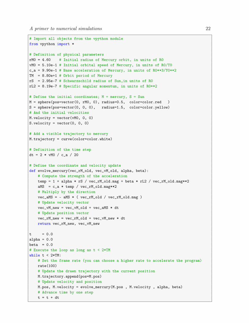
# Import all objects from the vpython modulefrom vpython import *

# Definition of physical parametersrM0 = 4.60 # Initial radius of Mercury orbit, in units of R0vM0 = 5.10e-1 # Initial orbital speed of Mercury, in units of R0/T0c_a = 9.90e-1 # Base acceleration of Mercury, in units of R0**3/T0**2TM = 8.80e+1 # Orbit period of MercuryrS = 2.95e-7 # Schwarzschild radius of Sun,in units of R0rL2 = 8.19e-7 # Specific angular momentum, in units of R0**2

# Define the initial coordinates; M = mercury, S = SunM = sphere(pos=vector(0, rM0, 0), radius=0.5, color=color.red )S = sphere(pos=vector(0, 0, 0), radius=1.5, color=color.yellow)# And the initial velocitiesM.velocity = vector(vM0, 0, 0)S.velocity = vector(0, 0, 0)

# Add a visible trajectory to mercuryM.trajectory = curve(color=color.white)

# Definition of the time stepdt = 2 * vM0 / c_a / 20

# Define the coordinate and velocity updatedef evolve_mercury(vec_rM_old, vec_vM_old, alpha, beta): # Compute the strength of the acceleration temp = 1 + alpha * rS / vec_rM_old.mag + beta * rL2 / vec_rM_old.mag**2 aMS = c_a * temp / vec_rM_old.mag**2 # Multiply by the direction vec_aMS = - aMS * ( vec_rM_old / vec_rM_old.mag ) # Update velocity vector vec_vM_new = vec_vM_old + vec_aMS * dt # Update position vector vec_rM_new = vec_rM_old + vec_vM_new * dt return vec_rM_new, vec_vM_new

t = 0.0alpha = 0.0beta = 0.0# Execute the loop as long as t < 2*TMwhile t < 2*TM: # Set the frame rate (you can choose a higher rate to accelerate the program) rate(100) # Update the drawn trajectory with the current position M.trajectory.append(pos=M.pos) # Update velocity and position M.pos, M.velocity = evolve_mercury(M.pos , M.velocity , alpha, beta) # Advance time by one step t = t + dt

A primer to numerical simulations: The perihelion motion ... · A primer to numerical simulations:...

Documents

Transcript of A primer to numerical simulations: The perihelion motion ... · A primer to numerical simulations:...