A Primer on Weather Forecasting

A Beginner’s Guide to Weather Forecasting and the Forecast Funnel

Patrick S. Market

Atmospheric Science Program Department of Soil, Environmental & Atmospheric Sciences

University of Missouri-Columbia

For Synoptic Meteorology I & II (ATMS-4710/-4720)

2008-2009

2

Contents

Introduction 4 Observations First… 5 …Forecasts Later 9 Temperature Forecasting 12 Precipitation Forecasting 15 Appendices Begin 17

© 2008 Patrick S. Market

3

Preamble Please note that this little text, and it is a text for this class, is by no means formal. It is also a living document that evolves from one year to the next, generally growing as more / better information becomes available, which is appropriate for the student forecaster. This booklet also exists at a time when modern operational (i.e. National Weather Service) forecasting is oriented less toward forecasting for points in space (like Columbia) and more oriented toward generating grids appropriate for a broad area. Nevertheless, we must walk before we can run, and learning to be a good “point” forecaster will be the first step on that journey.

4

Introduction This little tome is meant to give you an introduction to the science and art of

weather forecasting. While by no means exhaustive, it should give you some idea of how to

go about constructing a forecast based upon what you know about the atmosphere and the

use of both observed data and model output. By popular demand, recent additions include

more on process---with “how to” on forecasting variables such as temperatures, sky

condition, wind speed and direction, etc. These tend to be cookbook approaches to the

forecast, devoid of much dynamic understanding. However, they do tend to work and

also provide a means to produce a good forecast right from the start, even if you might not

always know why.

The idea is simple: if you know the current state of the atmosphere, you can then

make a prediction of its future state. To learn the present state of the atmosphere requires

many individual weather observations, preferably over the entire planet at both the surface

and aloft. We supplement these data with those from radar, satellites, and a host of other

platforms. But the basic process remains

1. Consult weather observations first, and

2. Create weather forecasts last.

Even simple folklore forecasting works this way. The old rhyme “Red sky at

night…” follows the process of making a prediction based upon some previous observation

of the atmosphere’s condition. While the science of meteorology has come a long way in the

last century, an “observations first” approach to the predictive process is still a valid one.

For instance, the profession of operational weather forecasting now has access to the output

from sophisticated computer-based numerical weather prediction (NWP) models. However,

5

the output from such models is imperfect and should never be a forecaster’s one and only

stop in the forecasting process. Think of yourself as a doctor, and the atmosphere as your

patient. You cannot make a prognosis for the patient without first making a thorough,

careful diagnosis of what is ailing him or her.

Observations First…

The first thing you should do is to acquaint yourself with what is going on with the

weather currently as well as over the last day or so. Once you’re into a daily forecasting

routine, you should have a good idea of what has gone on the last day or two and so can

proceed directly to looking at current data, charts, plots, etc. One of the hardest things to do

is to start forecasting: forecasters often have no “feel” for the weather when they have been

out of touch with maps, charts, talking with fellow forecasters, etc (away on vacation is a

good example).

Bottom line: Stay in touch! Come to the Map Wall and the WAV Lab daily and look

at the maps. While computer data feeds (Internet and in-house) are colorful and animated

and glitzy, they are unnecessary for establishing a synoptic understanding of the weather. The

need for snappy, psychedelic, up-to-the-minute data only becomes truly important on much

shorter time and space scales (such as when tornadoes and severe storms are threatening).

The paper charts on the Map Wall can serve as a focus for discussions between forecasters

and can also be re-analyzed and colored to suit you. Also, read the Missouri WFO

discussions (especially St. Louis, as we are in their CWA) and the products from NCEP

(such as the 1-2 Day discussion) daily. This will give you a sense of what other forecasters

are saying about your current, as well as impending, weather situation. As little as 20

6

minutes per day can keep you current on days when you’re not making a forecast. So, where

to begin?

Theory tells us that all smaller waves should derive their energy from much larger

waves. For example, a tornado may draw its energy from the larger mesocyclone that exists

inside the still-larger thunderstorm. The thunderstorm in question formed because of the

moisture, lift, and instability brought together within the even-larger extratropical cyclone

(“low pressure system”) in which the thunderstorm resides. So, in most instances, we should

begin by looking at the very largest scales (e.g., extratropical cyclones and larger) and then

finally working our way down to the very smallest scales (e.g., tornadoes). This approach is

known as “The Forecast Funnel.”

Globally

Start with the Northern Hemisphere analysis of 500-mb heights. Look over North

America and upstream over the Pacific Ocean. Is the planetary-scale flow more perturbed

(are there waves?) or is the flow zonal (generally west-to-east)? In the former case, your

weather may be slow to change, as the high wave

number may prohibit rapid storm motion.

However, if the wave number is fairly low (fewer

waves) as in the latter case, then the flow may be

more zonal and allow a more rapid propagation

of transient storm systems. This is not always

true, but it makes for a good rule of thumb, and a

place to start.

Figure 1. Example of a hemispheric analysis. Contours denote mean sea level pressure; shading defines 500-mb geopotential heights.

7

Nationally

Next, look at the US surface analysis. If you have the time, re-analyze the paper

chart in color; your pencils or markers will come in handy here. We will cover color

conventions for fronts, pressure systems, etc, as time goes on---until you’re sure of the

colors, just refrain from such re-analysis.

Anyway, what is going on? What is the

dominant system on the map? It may not

necessarily be a storm system, it may be an

enormous high pressure system. If it is a

storm system, what does a radar analysis

indicate? Is the system an active

precipitation producer?

Now look aloft, at the charts for 850 mb, 700 mb, 500 mb, etc. Do they look similar

to the surface chart? Well-developed systems (lows and highs) usually slope to the west with

height in the Northern Hemisphere. This means that for a low centered over, say, central

Missouri, good organization would find the 850 mb low over Kansas City, and central

Kansas at 500 mb, etc. Also, some guideposts to remember:

• 850 mb is especially good for identifying areas of moisture and low-level lift

• 500 mb is good for gauging the general nature of the flow and system

propagation

• 300 mb (250 mb in summer) is well-suited to identifying jet structures that

may encourage lift.

Also, there are many other charts that are available and address such matters as

Figure 2. Example of an HPC synoptic-scale surface analysis.

8

atmospheric stability, moisture, surface pressure changes, and the like. These can be

particularly valuable for assessing the motion of pressure systems, and their potential for

heavy precipitation, severe weather, etc. We will address many of these as the year

progresses.

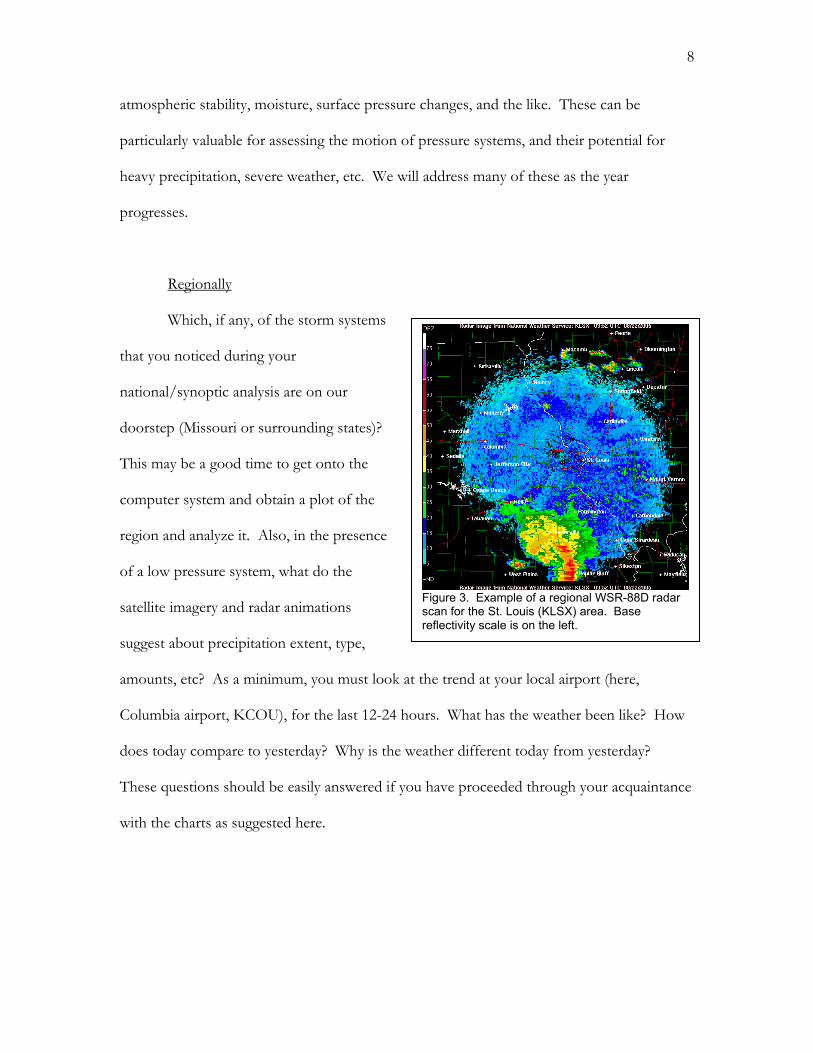
Regionally

Which, if any, of the storm systems

that you noticed during your

national/synoptic analysis are on our

doorstep (Missouri or surrounding states)?

This may be a good time to get onto the

computer system and obtain a plot of the

region and analyze it. Also, in the presence

of a low pressure system, what do the

satellite imagery and radar animations

suggest about precipitation extent, type,

amounts, etc? As a minimum, you must look at the trend at your local airport (here,

Columbia airport, KCOU), for the last 12-24 hours. What has the weather been like? How

does today compare to yesterday? Why is the weather different today from yesterday?

These questions should be easily answered if you have proceeded through your acquaintance

with the charts as suggested here.

Figure 3. Example of a regional WSR-88D radar scan for the St. Louis (KLSX) area. Base reflectivity scale is on the left.

9

… Forecasts Later

Now that you have familiarized yourself with what is and what has been, it is time to

look to the future. Before you look at any model output, ask yourself some questions:

• What, if anything, will be different between today and tomorrow?

o If nothing, a persistence forecast may do quite well.

What differentiates today from yesterday? Look at 24

hour temperature changes.

Why is today cooler/warmer than yesterday? Will this

trend continue?

o You may also want to modify persistence. For example, the

longer you spend in a given air mass, the more it will modify

from its original characteristics.

o Pay attention also to cloud arrival/departure. All other things

remaining the same, a sunny day tomorrow will be warmer than

the cloudy day today, and vice versa.

• Will my air mass be changing? How? When?

o A changing air mass usually denotes the passage of a front, which

is often the focus of active weather.

• Are the speed & direction of movement of the high/low/front changing?

Try to make a forecast first based upon what you know the weather has done over the last

day or so, and what it is doing at present. Then, and only then, should you proceed to

guidance products such as MOS and gridded model fields.

10

Model Output

You should proceed with your forecast process in the same manner as you did your

familiarization with the observations: globally nationally regionally locally. Most of

the standard operational model output is now available in-house by using GARP on the

department’s UNIX and Linux workstations. If you’re not in the lab, you may want go

online to http://weather.unisys.com where they have the basic fields available for the RUC,

NAM-WRF, NGM, GFS, and ECMWF Models. A useful progression may be to look at the

GFS or ECMWF first the GFS or NGM second the NAM-WRF and finally, the

RUC. Remember that you are attempting to assess the same sorts of things about the

atmosphere’s condition as when you first looked at the obs. However, here you are doing

this at various points in time in the future.

Some questions to ask yourself include:

• How does the model handle this system with each successive run? For

example, you may compare the 24 hour forecast from last night’s 00Z model

run with the 12 hour forecast from this morning’s 12 Z run. Two different

forecasts, but both valid at the same time. In the perfect world, these two

solutions will be identical. How close they come to one another is a measure

of model continuity.

• Also, how does the forecast from, say, the GFS model, compare to the

solutions for the same field at the same time from the NGM? How well

different simulation solutions compare from different models is a measure of

model consensus.

11

Model Output Statistics (MOS)

MOS is a method of correlating model output with observations and climatological

data to come up with tuned equations to refine forecasts of temperature, humidity, wind

velocity, visibility, precipitation probability, etc. An example of how to interpret a MOS

messages is detailed in Appendix B, and it is quite complete. My message here is more

cautionary in nature.

Be aware that MOS will give you everything that you need to make a forecast. It will

give you temperatures, wind shifts, lowered ceilings, precip types, precip amounts---just

about everything that a forecaster needs to make a good-looking forecast. But also beware of

its often-faulty nature. A good MOS forecast requires two things: first, that the model on

which the MOS is based arrived at a correct solution (not always the case) and secondly, that

during the period when scientists were correlating model output with observations etc., that

an event similar to the one you’re trying to forecast actually occurred (infrequent and record

events are never handled well by MOS).

In short, MOS is known as a guidance product, and should be treated as such.

MOS seldom, if ever, verifies better than a human forecaster if she/he is

1. properly trained and

2. putting forth an effort.

There will come days when you feel as though you just can’t improve on MOS; if so, then

use it. Yet, MOS is a guidepost, not a crutch. Don’t rely on it. Bottom line…

MOS is meteorological crack. Don’t become addicted to it.

12

Temperature Forecasting

As with most variables, forecasting the temperature is not nearly so mysterious a process as

it might seem. There are some “rules” that can be followed, and we will look at those

shortly. Yet, it is instructive to think through the process. Intuition tells us that if the

temperature today is 60°F, it is unlikely to be -10°F tomorrow; climatology provides bounds

on our thought process to keep us from going too wildly astray. At the same time, we also

know that if the temperature today is 60°F, it is unlikely to be 40°F tomorrow, unless a cold

front, for example, moves by your weather station.

In fact, a persistence approach is often tough to beat. If you are firmly within an air

mass, with no frontal zones expected to approach your forecast area in the next 48-72 hours

(common in the Midwest in summer), then what you experience on one day for a maximum

and minimum temperature may be an excellent prediction for the next day. You may want

to shade your max and min temperatures up a degree or two each day to allow your air mass

to modify, but that depends upon season, latitude, and the how recently frontal passage

occurred at the forecast location.

So, what can be done if a frontal zone is approaching? A common practice is to

look at surface analyses from the last several days and track the front that is approaching or

has just passed your location. Let’s use a cold front as an example. The goal here is to find

an upstream weather station that was about as far behind the cold front yesterday as your

station will be today. The 24-hour difference between the max temperature yesterday and

the max temperature two days prior at the upstream location is a good estimate for the

temperature change between yesterday and today at your target forecast station. An example

of this approach is shown in the Figure 4.

13

A few rules and tips…

• To estimate the afternoon maximum temperature

o find the temperature at 850 mb on the morning (12Z) sounding and mix it

down, dry adiabatically, to the surface (not sea level, unless you are

forecasting for a sea level location). The surface value is your estimate of

the daytime maximum temperature.

o Works best for

mid-latitude locations

Figure 4. Example of forecasting temperature (in this case, the maximum) using the steady-state motion of a frontal zone. The solid front labeled “T-24” represents an observed frontal zone location 24-hours prior to your analysis of the current frontal zone (the solid one in the middle, labeled “T-00”). The broken frontal zone labeled “T+24” denotes the forecast position of the same frontal zone 24-hours into the future. “X” is the station for which you will calculate the difference between the max temperatures from two days ago and one day ago. “O” is the station for which you are forecasting; subtract the difference in ΔTmax between Day 2 and Day 1at “X” from yesterday’s maximum temperature at “O” as a first guess for today’s max.

14

the warm season

times when partly sunny or better conditions are expected .

o ***However, while 850-mb air may be too high to mix down in the winter,

850-mb may not be high enough from which to mix in the summer.

• To estimate the overnight minimum temperature

o determine the dew point at the time that the air temperature reaches its

maximum.

works best on partly sunny (or better) days

This dew point value is a good estimate of the overnight

minimum temperature.

o The strongest radiational cooling tends to occur just after sunset. This idea is

most effective when the sun sets under a (nearly) clear sky, as opposed to a

cloudy sunset. Of course, a sunset with a clear sky does not mean that

clouds can not approach overnight. Read on…

o Increasing cloud cover during the overnight hours can halt cooling, and even

cause a few degrees of warming as the clouds roll in.

15

Precipitation Forecasting

Forecasting precipitation also tends to be a straightforward process. In order for

precipitation to reach the ground, a cloud is necessary for its formation. At its most

fundamental level, then, sufficient moisture is necessary not only for cloud creation, but also

precipitation production. Of course, a great deal of water vapor only ensures saturation --- a

cloud aloft or fog at the surface. In order for precipitation to form, it is generally true that

atmospheric parcels should also be actively ascending.

A well-known rule of thumb is that at 700 mb (about 10,000 feet above mean sea

level, and a level representative of the lower- to mid-troposphere), -1 μb s-1 equates to about

+1 cm s-1. For example, if we observe -10 μb s-1 in output from a reliable forecast model, then

we can expect a parcel with that vertical velocity to ascend 360 meters in a single hour, or

about 1 km in 3 hours! If this ascent occurs in unsaturated air, then we need not expect

cloud formation or precipitation production. If the air is moist (preferably saturated or

nearly so), then cloud production and precipitation are much more likely. An ideal situation

would have an upward vertical motion (< -5 μb s-1) area at 700 mb co-located with an area of

significant moisture (RH > 90%) at that same level. Of course, evaluation of moisture over

a layer is usually preferable to examining just at a single level. In the following example (Fig.

5), we look at a typical extratropical cyclone (Fig. 5a) and we also compare the vertical

motion at 700 mb to the averaged relative humidity (Fig. 5b) over a layer from 1000-500 mb

(from the surface to ~18,000 feet above mean sea level). The resulting precipitation field

predicted by the model (Fig. 5c) is shown for the 6-hour period that ensues after the analyses

shown in Figs. 5a and 5b.

16

Of particular interest is the region in central Quebec, southeast of the southern tip of

Hudson Bay. Focused along and just north of a surface warm front, a deep layer with

relative humidity > 90% coincides with a region where the vertical motions are < -5 μb s-1

over a large area (Fig. 5b). Notice that a large region of significant precipitation occurs over

that region as well as toward the east-northeast (following the motion of the storm system).

We could simply use the precipitation field to produce our forecast, but using the approach

discussed here allows us to form a hypothesis (i.e. copious moisture and strong upward

motion should lead to rainfall) and then test it to see if it is true (does the model put

precipitation where the moisture and rising motions occur?)

a b

c Figure 5. a) Sea level pressure (every 4 mb; green, solid) and 1000-500-mb thickness (every 60 gpm; brown; dashed), b) relative humidity (shaded) and vertical motion (every 5 μb s-1 ; dashed, yellow), and c) the 6-hour model forecast of precipitation for the 6-hour period after the analysis snapshots that we see in a) and b).

17

Appendix A

AFD Area Forecast Discussion

AWC Aviation Weather Center

CWA - County Warning Area

GARP - GEMPAK Analysis and Rendering Program

GEMPAK - GEneral Meteorological PAcKage

HPC Hydrometeorological Prediction Center

MOS - Model Output Statistics

NCEP - National Centers for Environmental Prediction

NHC National Hurricane Center

SPC Storm Prediction Center

TPC Tropical Prediction Center

WAV Lab - Weather Analysis and Visualization Laboratory (MU)

WFO - Warning and Forecast Office

AVN - AViatioN model (a historical name; phasing out)

ETA - Eta model (a historical name; forerunner to the NAM)

ECWMF - European Centre for Medium-Range Weather Forecasting

GFS - Global Forecasting System

MASS - Mesoscale Atmospheric Simulation System

MRF - Medium Range Forecast (a historical name; phasing out)

NAM North American Mesoscale model

NGM - Nested Grid Model

18

RUC - Rapid Update Cycle (model)

UKMET - United Kingdom Meteorological Office model

WRF - Weather Research and Forecasting model

19

Appendix B

NGM MOS Message Explanation

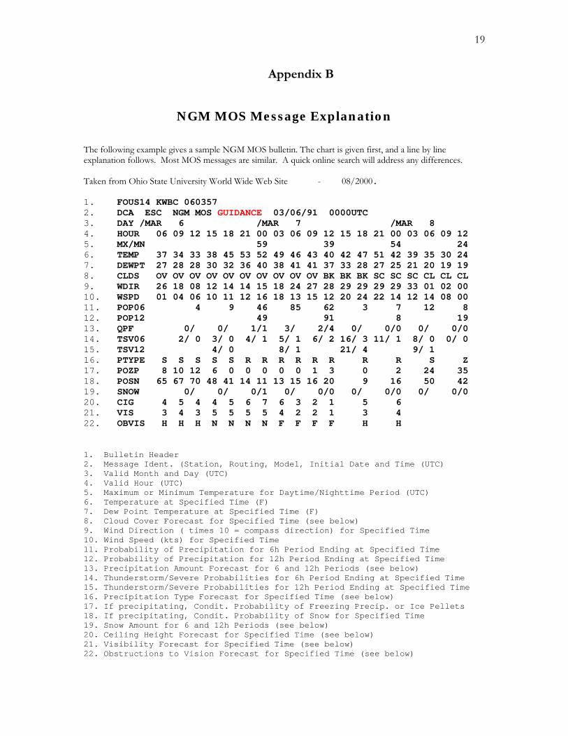
The following example gives a sample NGM MOS bulletin. The chart is given first, and a line by line explanation follows. Most MOS messages are similar. A quick online search will address any differences. Taken from Ohio State University World Wide Web Site - 08/2000. 1. FOUS14 KWBC 060357 2. DCA ESC NGM MOS GUIDANCE 03/06/91 0000UTC 3. DAY /MAR 6 /MAR 7 /MAR 8 4. HOUR 06 09 12 15 18 21 00 03 06 09 12 15 18 21 00 03 06 09 12 5. MX/MN 59 39 54 24 6. TEMP 37 34 33 38 45 53 52 49 46 43 40 42 47 51 42 39 35 30 24 7. DEWPT 27 28 28 30 32 36 40 38 41 41 37 33 28 27 25 21 20 19 19 8. CLDS OV OV OV OV OV OV OV OV OV OV BK BK BK SC SC SC CL CL CL 9. WDIR 26 18 08 12 14 14 15 18 24 27 28 29 29 29 29 33 01 02 00 10. WSPD 01 04 06 10 11 12 16 18 13 15 12 20 24 22 14 12 14 08 00 11. POP06 4 9 46 85 62 3 7 12 8 12. POP12 49 91 8 19 13. QPF 0/ 0/ 1/1 3/ 2/4 0/ 0/0 0/ 0/0 14. TSV06 2/ 0 3/ 0 4/ 1 5/ 1 6/ 2 16/ 3 11/ 1 8/ 0 0/ 0 15. TSV12 4/ 0 8/ 1 21/ 4 9/ 1 16. PTYPE S S S S S R R R R R R R R S Z 17. POZP 8 10 12 6 0 0 0 0 0 1 3 0 2 24 35 18. POSN 65 67 70 48 41 14 11 13 15 16 20 9 16 50 42 19. SNOW 0/ 0/ 0/1 0/ 0/0 0/ 0/0 0/ 0/0 20. CIG 4 5 4 4 5 6 7 6 3 2 1 5 6 21. VIS 3 4 3 5 5 5 5 4 2 2 1 3 4 22. OBVIS H H H N N N N F F F F H H 1. Bulletin Header 2. Message Ident. (Station, Routing, Model, Initial Date and Time (UTC) 3. Valid Month and Day (UTC) 4. Valid Hour (UTC) 5. Maximum or Minimum Temperature for Daytime/Nighttime Period (UTC) 6. Temperature at Specified Time (F) 7. Dew Point Temperature at Specified Time (F) 8. Cloud Cover Forecast for Specified Time (see below) 9. Wind Direction ( times 10 = compass direction) for Specified Time 10. Wind Speed (kts) for Specified Time 11. Probability of Precipitation for 6h Period Ending at Specified Time 12. Probability of Precipitation for 12h Period Ending at Specified Time 13. Precipitation Amount Forecast for 6 and 12h Periods (see below) 14. Thunderstorm/Severe Probabilities for 6h Period Ending at Specified Time 15. Thunderstorm/Severe Probabilities for 12h Period Ending at Specified Time 16. Precipitation Type Forecast for Specified Time (see below) 17. If precipitating, Condit. Probability of Freezing Precip. or Ice Pellets 18. If precipitating, Condit. Probability of Snow for Specified Time 19. Snow Amount for 6 and 12h Periods (see below) 20. Ceiling Height Forecast for Specified Time (see below) 21. Visibility Forecast for Specified Time (see below) 22. Obstructions to Vision Forecast for Specified Time (see below)

20

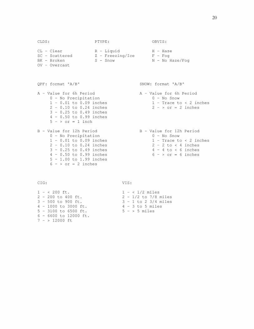
CLDS: PTYPE: OBVIS: CL - Clear R - Liquid H - Haze SC - Scattered Z - Freezing/Ice F - Fog BK - Broken S - Snow N - No Haze/Fog OV - Overcast QPF: format "A/B" SNOW: format "A/B" A - Value for 6h Period A - Value for 6h Period 0 - No Precipitation 0 - No Snow 1 - 0.01 to 0.09 inches 1 - Trace to < 2 inches 2 - 0.10 to 0.24 inches 2 - > or = 2 inches 3 - 0.25 to 0.49 inches 4 - 0.50 to 0.99 inches 5 - > or = 1 inch B - Value for 12h Period B - Value for 12h Period 0 - No Precipitation 0 - No Snow 1 - 0.01 to 0.09 inches 1 - Trace to < 2 inches 2 - 0.10 to 0.24 inches 2 - 2 to < 4 inches 3 - 0.25 to 0.49 inches 4 - 4 to < 6 inches 4 - 0.50 to 0.99 inches 6 - > or = 6 inches 5 - 1.00 to 1.99 inches 6 - > or = 2 inches CIG: VIS: 1 - < 200 ft. 1 - < 1/2 miles 2 - 200 to 400 ft. 2 - 1/2 to 7/8 miles 3 - 500 to 900 ft. 3 - 1 to 2 3/4 miles 4 - 1000 to 3000 ft. 4 - 3 to 5 miles 5 - 3100 to 6500 ft. 5 - > 5 miles 6 - 6600 to 12000 ft. 7 - > 12000 ft

21

Appendix C

HPC Basic Weather Symbology

- from the HPC website

22

Appendix D

HPC Frontal Symbols

The final word on real-time, operational surface analyses comes from the HPC. Below is a guide to the symbology and coding used by HPC for each analysis.

- from the HPC website

Key to Features 1 -- Cold Front 2 -- Warm Front 3 -- Stationary Front 4 -- Occluded Front 5 -- Trough ("TROF") Also used to depict Outflow Boundary ("OUTFLOW BNDRY") 6 -- Squall Line 7 -- Dry Line 8 -- Tropical Wave ("TRPCL WAVE") Each surface front and squall line (1, 2, 3, 4, 6 above) is accompanied by a 3-digit label that has a bracket

either before or after it. Using the example "[ABC", here is how to translate the label: A: Type of Front B: Strength of Front C: Other Characteristics 0 = stationary 0 = none (applies only to squall line) 0 = none 2 = warm 1 = weak, weakening 5 = forming 4 = cold 2 = weak 6 = quasi-stationary 6 = occluded 3 = weak, strengthening 7 = with waves 7 = squall line 4 = moderate, weakening 8 = diffuse

5 = moderate 6 = moderate, strengthening 7 = strong, weakening 8 = strong 9 = strong, strengthening

23

Eastern United States Military Stations

Appendix E1

ID Station Location ID Station Location KADW Andrews AFB, Camp Springs, MD KAEX England AFB, Alexandria, LA KBAD Barksdale AFB, Shreveport, LA KBIX Keesler AFB, Biloxi, MS KBLV Scott AFB, Belleville, IL KCBM Columbus AFB, MS KCEF Westover AFB, Holyoke, MA KCOF Patrick AFB, Melbourne, FL KDAA Ft. Belvoir, Engleside, VA KDOV Dover AFB, DE KFAF Ft. Eustis, Newport News, VA KFBG Ft. Bragg, Fayetteville, NC KFFO Wright-Patterson AFB, Dayton, OH KFMH Falmouth, MA KFTK Ft. Knox, KY KGSB Seymour-Johnson AFB, Goldboro, NC KGUS Grissom AFB, Kokomo, IN KHRT Hurlburt Field (AF), FL KHOP Ft. Campbell, Clarksville, TN KLCK Lockborne AFB, Columbus, OH KHST Homestead AFB, FL KLHW Ft. Stewart, Hanesville, VA KLFI Langley AFB, Hampton, VA KLSF Ft. Benning, Columbus, GA KLRF Little Rock AFB, AR KMGE Dobbins AFB, Atlanta, GA KMCF Macdill AFB, Tampa, VA KMTC Selfidge AFB, Roseville, MI KMMT McEntire, SC KMUI Muir AAF, Fort Indiantown Gap, PA KMTN Martin Airfield, Baltimore, MD KMYR Myrtle Beach AFB, SC KMXF Maxwell AFB, Montgomery, AL KNCA MCAS New River, Jacksonville, NC KNBC MCAS Beaufort, SC KNGU NAS Norfolk, VA KNEL NAS Lakehurst, NJ KNIP NAS Jacksonville, FL KNHK NAS Patuxent River, MD KNMM NAS Meridian, MS KNKT MCAS Cherry Point, NC KNQA NAS Memphis, TN KNPA NAS Pensacola, FL KNRB Mayport NS, Jacksonville, FL KNQX NAS Key West, FL KNTU NAS Oceana, Virginia Beach, VA KNSE NAS Whiting Field, FL KNYG MCAS Quantico, VA KNXX NAS Willow Grove, PA KPAM Tyndall AFB, Panama City, FL KOZR Ft. Rucker, Ozark, AL KPOE Camp Polk, Leesville, LA KPOB Pope AFB, Fayetteville, NC KSSC Shaw AFB, Sumters, SC KPSM Pease AFB, Portsmith, NH KTBN Ft. Leonard Wood, Waynesville, MO KSZL Whiteman AFB, Sedalia, MO KVPS Eglin AFB, Valparaiso, FL KVAD Moody AFB, Valdosta, GA KWRI McGuire AFB, Browns Mills, NJ KWRB Warner Robbins AFB, Macon, GA

24

Western United States Military Stations

Appendix E2

ID Station Location ID Station Location KBAB Beale AFB, Marysville, CA KNUQ Moffet NAS, San Jose, CA KBKF Buckley AFB, Denver, CO KNUW Whidbey Is. NAS, WA KCVS Cannon AFB, Clovis, NM KNZY North Is. NAS, San Diego, CA KDLF Laughlin AFB, Abilene, TX KOFF Offutt AFB, Omaha, NE KDMA Davis Monthan AFB, Tucson, AZ KRCA Ellsworth AFB, Rapid City, SD KDYS Dyess AFB, Abilene, TX KRDR Grand Forks AFB, ND KEDW Edwards AFB, N. Edwards, CA KRIV March AFB, Riverside, CA KEFD Ellington AFB, Houston, TX KRND Randolph AFB, San Antonio, TX KEND Vance AFB, Enid, OK KSKA Fairchild AFB, Spokane, WA KFCS Ft. Carson, Colorado Springs, CO KSKF Kelly AFB, San Antonio, TX KFOE Forbes AFB, Topeka, KS KSUU Travis AFB, Fairfield, CA KFRI Ft. Riley, Marshall, KS KTCM McChord AFB, Tacoma, WA KFSI Ft. Sill, OK KTIK Tinker AFB, OK KGRF Ft. Lewis, Lakewood Center, WA KVBG Vandenberg AFB, Lompoc, CA KGRK Ft. Hood, Killeen, TX KHIF Hill AFB, Ogden, UT KHMN Lolloman AFB, Alamosa, NM KIAB McConnell AFB, Wichita, KS KLSV Nellis AFB, Las Vegas, NV KLTS Altus AFB, OK KLUF Luke AFB, Phoenix, AZ KMIB Minot AFB, ND KMUO Mountain Home AFB, ID KNFL Fallon NAS, NV KNGP Corpus Christi NAS, TX KNID China Lake NAS, Ridgecrest, CA KNKX Miramar, NAS, San Diego, CA KNQI Lemoore NAS, Reeves, CA KNRS Imperial Beach NAS, CA KNSI San Nicolas Is., CA KNTD Pt. Mugu NAS, Oxnard, CA

25

Appendix F

Adding Color to the CWF We can still be accurate while painting a more vivid picture of the forecast. What follows is a list of phrases (some overlooked, some goofy, many co-opted from friends and colleagues) that you might try out to make the forecast more readable or illustrative. I have also included some commonly-used phrases that are vague (Try to Avoid), and suggest that your confidence in a given forecast is lower than usual. Where possible, do not use them in the first 3 periods. Temperatures Frigid Frosty Temperatures near the record of… Arctic-like conditions Boiling heat Near-record heat Near-record cold Balmy Temperatures will rise Temperatures will soar Steady or slowly falling temperatures Steady or slowly rising temperatures (usually after an overnight or early day cold frontal passage) (usually after an overnight or early eve. warm frontal

passage) Precipitation Occasional showers Gusty thunderstorms Wind-swept showers Stray thunderstorm Stray shower Passing shower Risk of a shower Watch for a shower Hit or miss thunderstorm Watch for a shower Shower in one or two spots Intermittent rain Spotty drizzle Periods of rain On and off rain A cold rain A few hours of rain Humidity Tropical Tropic-like conditions Hot and humid Sticky Muggy Steamy Oppressive Clammy Damp and dreary Sky condition Bright sunshine Abundant sunshine Hazy sunshine Crystal clear Moonlit skies Sun through high clouds Starry skies Overcast Winds Breezy Refreshing breeze Gusty Blustery Fog/Visibility Fog in low-lying areas Patchy fog Dense fog Valley Fog General Summer-like Winter-like A mix of sun and clouds Pleasant Fall-like Spring-like A mix of clouds and sun Try to Avoid (especially in the early periods) Variable cloudiness Showers possible Some sunshine Some cloudiness Changeable skies Chance of showers Chance of snow Possible showers

26

Appendix G

FOUR IMPORTANT FORECASTING CONCEPTS (Modified from “A Guide to Weather Forecasting” by E. Horst, ©1990)

CONSENSUS forecasting almost always yields the best forecast. This can be consensus of the different computer model forecasts or consensus of individual forecasters. Both are important; however, the latter is critical. Studies have shown that a group of “average” forecasters can usually out-forecast a single “expert” forecaster. So before you post your forecast, always try to have a brief map discussion with some other “in-touch” forecasters. If none are around you can always call up the NWS discussion and forecast for our area (LSX and EAX, and even SGF depending upon the flow regime). CONTINUITY is critical for accuracy and credibility! What this means is that you should have a good reason to make changes when you are updating the forecast. If you think a big change is necessary, discuss it with another person or with the previous forecaster (what was their thinking?). This is why leaving a forecast message for those forecasting on the shift after yours is so important. Also, minor changes of wording are fine; however, minor changes of temperature are bad. One degree changes are taboo! Simply put, a constantly changing forecast gives the public the impression that you don't have a clue. It also minimizes your chances of verifying. Example: If you think the previous temperature forecast (Low: 36 - 40) is off by just a degree or two, then don't change it! If you think that the forecast is off by more than two degrees, then do change it! However, you can still partially preserve continuity by keeping one of the previous forecast's temperatures in your new forecast. If the old forecast was “Low: 36 – 40”, then the best changes (preserving continuity) would be “Low near 36”, “Low near 40”, “Low: 32 – 36”, or “Low: 40 – 44”. All of these revised temperature forecasts contain part of the old forecast! Again, one thing that you never want to do is make a one-degree change. In the case above, you WOULDN'T EVER want to revise “Low: 36-40” to “Low: 35”, “Low 35 – 39”, “Low: 37”, “Low: 37 – 41”, “Low: 39”, “Low: 39 – 43”, or “Low near 41”. The numbers 35, 37, 39, 41 are now off limits. By using any of those four numbers in your revision, you are making a one degree change, which, if you think about it, is absurd. How can you claim that, by looking at the guidance, you're able to note a one-degree change, particularly beyond the first few periods? PERSISTENCE forecasting can be quite useful, especially in slow-moving or stagnant weather patterns. For instance, when there's a stubborn high pressure in the east, it's not uncommon for our high and low temperature to be almost the same for several days in a row. Consequently, your best temperature guidance is a quick look at the previous day's

27

high and low! In many cases a slight change of persistence will give you a great forecast. An example would be when a Canadian high pressure drops over our area. The first full day under the high is generally the coolest, but on each successive day the air mass is modified. Consequently, you can take the first day's high temperature and adjust it a bit (up or down) according to the change in the air mass (adjust for clouds, winds, dew points, etc.). FUDGE PHRASES, if used sparingly, are useful in achieving high “error avoidance”. Fudge phrases, also known as “sleaze lines,” are not necessarily bad. In reality, all forecasters use them whether they know it or not---in fact, many forecasters use them TOO MUCH. By using a fudge phrase correctly, you not only give yourself the best chance at avoiding a bust, but you also portray to the public the true uncertainty in such a way that they don't realize that you're uncertain! Common fudge phrases are “variable cloudiness” (VC), “changeable skies”, “some sunshine”, and even “chance of showers”. What are the above lines actually saying? They are saying (in a nice way) that you really aren't sure what's going to happen. If that is actually the case, then use a fudge phrase (for days 2 or 3); if that's not the case and you really are confident about what's happening, then DON'T use a fudge phrase.