A PREDICTIVE MODEL FOR THE DAILY EXCHANGE...
22
Lebanese Science Journal, Vol. 14, No. 2, 2013 93 A PREDICTIVE MODEL FOR THE DAILY EXCHANGE RATE OF THE EUR/USD USING MARKOV CHAIN AND COINTEGRATION TECHNIQUES Mahmoud Mourad and Ali Harb 1 Department of Economics, Faculty of Economic Sciences and Business Administration (Branch V), Lebanese University, Lebanon 1 Department of Mathematics, Faculty of Sciences (Branch V), Lebanese University, Lebanon [email protected] (Received 9 May 2013 - Accepted 24 June 2013) ABSTRACT This paper adds to the literature of the exchange rates, some practical points which will be of great importance for financial markets and especially for the stock market. Firstly, the daily alternation of High and Low on the exchange rates ofEUR/USD follows a uniform distribution and hence if someone bets on this alternation then he puts himself in a position of maximum uncertainty. Secondly, buying and selling always represent the care for the speculators seeking the right time to open or close their operations. Any decision deprived of necessary information of the exchange rate (market prices) and especially their volatility, leads to a high risk and the probability of failure of such a speculator is highly elevated. The four variables Open, High, Low and Close are stationary in first difference. Since the variables High and Low determine completely the daily extent of the exchange rate EUR/USD, one focused on their evolution taking into account the volatility resulting from an ARCH effect. For these two variables, one performs a measurement of risk using the family of ARCH models such as ARCH-M, EARCH symmetric and asymmetric and GJR-EARCH asymmetric. Thirdly, one presents an analysis of cointegration regression for the four systems of variables (High, Open), (Low, Open) and (High, Low, Open) and (High, Low, Open, Close). Therefore, the Open variable is very informative for those four systems because its value is known at the opening of the market, so it could be served as an endogenous and exogenous variable. Finally, one predicts prices and volatility of the high and Low using the (ECM) models associated to the two first systems and one shows that the ex-post forecasts reveal an excellent performance. Keywords: exchange rates, stationary, Markov chain, ARCH, cointegration, forecasts INTRODUCTION After the Second World War, the USA was one of the first winners, and each country of this planet began to focus on the urban development and the economic and financial prosperity. The U.S. dollar became the most sought currency in the world. Actually, the U.S. economy recorded a GDP of USD 14 991.3 billion (Source World Bank 2011) in 2011, 21.42% of the world GDP evaluated at USD 69 981.9 billion at current prices and
Transcript of A PREDICTIVE MODEL FOR THE DAILY EXCHANGE...
Lebanese Science Journal, Vol. 14, No. 2, 2013 93
A PREDICTIVE MODEL FOR THE DAILY
EXCHANGE RATE OF THE EUR/USD USING
MARKOV CHAIN AND COINTEGRATION
TECHNIQUES
Mahmoud Mourad and Ali Harb1
Department of Economics, Faculty of Economic Sciences and Business Administration
(Branch V), Lebanese University, Lebanon 1Department of Mathematics, Faculty of Sciences (Branch V), Lebanese University, Lebanon
(Received 9 May 2013 - Accepted 24 June 2013)
ABSTRACT
This paper adds to the literature of the exchange rates, some practical points which
will be of great importance for financial markets and especially for the stock market. Firstly,
the daily alternation of High and Low on the exchange rates ofEUR/USD follows a uniform
distribution and hence if someone bets on this alternation then he puts himself in a position of
maximum uncertainty. Secondly, buying and selling always represent the care for the
speculators seeking the right time to open or close their operations. Any decision deprived of
necessary information of the exchange rate (market prices) and especially their volatility,
leads to a high risk and the probability of failure of such a speculator is highly elevated. The
four variables Open, High, Low and Close are stationary in first difference. Since the
variables High and Low determine completely the daily extent of the exchange rate
EUR/USD, one focused on their evolution taking into account the volatility resulting from an
ARCH effect. For these two variables, one performs a measurement of risk using the family of
ARCH models such as ARCH-M, EARCH symmetric and asymmetric and GJR-EARCH
asymmetric. Thirdly, one presents an analysis of cointegration regression for the four systems
of variables (High, Open), (Low, Open) and (High, Low, Open) and (High, Low, Open,
Close). Therefore, the Open variable is very informative for those four systems because its
value is known at the opening of the market, so it could be served as an endogenous and
exogenous variable. Finally, one predicts prices and volatility of the high and Low using the
(ECM) models associated to the two first systems and one shows that the ex-post forecasts
reveal an excellent performance.
Keywords: exchange rates, stationary, Markov chain, ARCH, cointegration, forecasts
INTRODUCTION
After the Second World War, the USA was one of the first winners, and each
country of this planet began to focus on the urban development and the economic and
financial prosperity. The U.S. dollar became the most sought currency in the world. Actually,
the U.S. economy recorded a GDP of USD 14 991.3 billion (Source World Bank 2011) in
2011, 21.42% of the world GDP evaluated at USD 69 981.9 billion at current prices and
Lebanese Science Journal, Vol. 14, No. 2, 2013 94
18.54% of the world GDP (PPP) evaluated to 80 855.211 billion. A nation's GDP at
purchasing power parity (PPP) exchange rates is the sum value of all goods and services
produced in the country valued at prices prevailing in the United States. The importance of
the U.S. dollar is in attempting international comparison of exchange rates or GDP in current
international dollars. Indeed, the current international dollar has now become a unit of
reference in the world. The start of the euro as a rival currency to the USD has pushed all
countries to focus on the exchange rate between the two currencies and many theoretical and
practical studies have been done in order to try to give proper answers on the changes in the
financial market where the stock market is its main axis. Actually, the European Union (EU)
is an economic and political union of 27 member states where 17 countries have adopted the
euro as a single currency. In 2011, the GDP (PPP) is 16441,916 billion, or 20.33% of the
world GDP (PPP). This new state of the world economy has made the foreign exchange
market between the euro and the dollar one of the most active ones in the world. In fact, the
EUR / USD rate is the most financial instrument traded in the world. It is a leading indicator,
daily followed by all economic and financial circles. This parity is calculated moment by
moment, while the following four indicators of market movement are present: Open, High,
Low and Close. The exchange rates EUR/USD have a great importance for the economy of a
country, especially for its foreign trade. For example, suppose that the euro appreciates
against the dollar, that is, the exchange rate EUR/USD increases from 1 € = $ 1.3020 to 1 € =
$ 1.4020 a few months later, then the products exported by the United States to the countries
of the Euro zone will be more competitive. Conversely, exports from the euro zone will have
a higher price in USD and will be less competitive in the U.S. compared to local products.
The price of EUR / USD move freely in a floating exchange rate, depending on the supply
and demand in the interbank market. Allegret (2007) studies and outlines the main advantages
and disadvantages of different exchange rate regimes and concludes that the intermediate
regimes seem a better solution for emerging countries. Dunis et al. (2008) studied the
forecasting and trading of the daily (EUR/USD) exchange rate using the European Central
Bank (ECB) fixing series with only autoregressive terms as inputs. Bénassy-Quéré et al.
(2009) propose an illustration for the euro/dollar exchange rate and suggest that the various
approaches1 should be combined to provide useful benchmarks for exchange-rate policies.
In this research, the exchange rates of EUR / USD are available hour by hour, day
by day, and month by month. One has two data files: (F1) of 65 328 hours in spot value, that
is 2722 days are full, 24 hours per day2, and another data file (F2) of size 2800 days (5 days
per week without missing days, Monday to Friday) covering the period September 29, 2000
until November 16, 20113.
The choice of these two files is justified by this objective that consists in performing
two types of analysis: first type, the F1 file was used to identify for each day, the time of
1Purchasing power parity (PPP), Behavioral Equilibrium Exchange Rate (BEER) and
Fundamental Equilibrium Exchange Rate (FEER). 2We selected only the full days with 24 hours of trade. 3The foreign exchange market, which is usually known as "forex" or "FX," is the largest
financial market in the world. The source of the data sets is from the Forex Time (FXTM)
company whichgives us access to the forex market 24 hours a day, 5 days a week, allowing us
to trade over 60 currency pairs.
Lebanese Science Journal, Vol. 14, No. 2, 2013 95
emergence of High and Low, and the distance time between them. Indeed, for market
speculation, many speculators believe the almost deterministic alternating between High and
Low. For example, in the first Friday of each month, the day of the meeting with the media,
of Ben Shalom Bernanke, Chairman of the Federal Reserve, the central bank of the United
States (Fed), and hence the realization of High or Low results of his declaration. One
considers only the full days of 24 hours are the days in which the High and Low are
theoretically equally likely to be observed. The important question that arises here is the
following: which of the two variables is more likely to occur firstly in a day of 24 hours? This
file will allow one, therefore, to search the times of High and Low through 24 hours of a full
day, and to quantify this "alternation" between the High and Low. Another possible use of this
file (F1) lies in the determination of the range of the time between the daily achievements of
the High and Low. What is the law of this range? A question that certainly deserves a proper
answer. To study the dual system for the High and the Low, one introduces a dummy variable
of alternating High (DAH) with two integer values: 1 if the High occurs first in a day and 0
otherwise. It is clear that the two alternating systems are equivalent and hence one can just
study the High system. To achieve this goal, one will use the technique of the Markov chain
at first order. This work will allow one to estimate, in one hand, the two-state Markov model
and in the other hand, to consider the long-term balance of probabilities states. It is clear that
this system has two states consisting of the emerging of the High or not. Second type, it
should be noted here that the file (F2) was introduced without missing data covering the
period 01/01/2001 - 23/09/2011 (2800 days). Indeed, the time series contains 5 holidays
whose values were estimated by the moving average smoothing technique. This series will be
analyzed by the techniques of "family" ARCH and cointegration between the High and Low
taking the variable Open as an exogenous variable because its value is known at the time of
the opening of the market. It will be very interesting to introduce the opening value of the
EUR/USD at the present time as an explanatory variable for dependent variable (High or
Low). In fact this available information will have an impact to reduce the fluctuations in the
Exchange Rate Market. This paper consists of an introduction, of three main areas and a
conclusion. In the second section, one uses the technique of Markov chain at first order to
carry out a study of the daily alternation of the variables high and low of the exchange rate
EUR / USD. In the third section, a modeling volatility of the exchange rate will be developed
using the conditional variance, a fundamental objective for the technical ARCH models. In
the fourth section, a detailed analysis of the cointegration regression is performed by
examining four systems choosing 2, 3 and 4 of the variables Open, Low, High and Close.
Finally, one presents a conclusion based on the various results that are obtained earlier.
MARKOV ANALYSIS OF ALTERNATION HIGH SYSTEM
The discrete-time Markov chains at first order is a special case of all Markov
stochastic processes ( ) , I is called the state-space. The amount of information stored in
the past at lag one influences its nearest future. Indeed, for a Markov chain, the information at
a time t guides the observation at the next time. In other words, the Markov chains have no
memory (Morris 1997) because the state of the system at the time t is the " crossing bridge"
that leads its state at time t+1. For , conditional probability on , has distribution
( ), and is independent of where has a known distribution. Explicitly
one can write:
( | ) (R1)
Lebanese Science Journal, Vol. 14, No. 2, 2013 96
The matrix ( ) is stochastic because every row ( ) is a
distribution ( ∑ ). In most economic and social phenomena, one notes
that the information progress in the time that moves forward and not backward (forward-
looking), and hence the idea that time moves forward and not backward is quite current and
familiar.
The discrete-time Markov chains is specified if one specifies the transition
probabilities between a state i at the time t and the state j at the time t+1. If the state-space
is finite and contains (s) states, the matrix P verifies:
( ) where all , ∑
and ∑
.
A discrete-time Markov chain will therefore be completely defined by the data of
the transition matrix P and by the state at the initial time. In addition, if for all coprime
integers n such that , then the Markov chain is called ergodic. In this regard, one
directs the reader to Morris (1997). This ergodic theorem identifies the proportion of long-
term time spent in each state. A Markov chain is called irreducible if for every pair of states
(i, j), the probability of going from one to the other is strictly positive. It is called to be
periodic of period m, if the trajectory returns to the initial state after m steps, that is
. If after a number of iterations, tends to a limit matrix whose columns are all
equal, which means that the distribution (proportion of each state) evolves into a single
distribution which is a stationary distribution. The Markov chain is said to be stationary or
homogeneous if the transition probability between state i at time t and the state j at time t+m
depends only on the extent of the time (Papoulis, 1986) and so one obtains:
( | ) ( ) and one can prove that the associated transition matrix is
( ) ( ) ( )
This means that the transition probability from one state to another
in m movements are simply obtained by the matrix P to the power m. In general, one can
write . In this case, the Markov chain is finite because the state-
space contains two elements (1 and 0). The transition matrix P is given by
P = (
) , and
Where ( | ) and ( | ).The matrix P is assumed to
be regular, that is, there exists an integer m such that the elements of the matrix are all
positive. Let be the vector of state probabilities, that is, ( ) Obviously, one of the
purposes of Markov analysis is to predict the future. Furthermore if one is in any period t, the
state probabilities for period t+1 can be computed as follows:
(R2)
Thus one can compute the equilibrium state probabilities. An equilibrium condition
exists if the state probabilities do not change after a large number of periods. Thus, at the
equilibrium, the state probabilities for a future period must be the same as the state
probabilities for the current period (Render et al., 1994). This fact is the key to finding the
equilibrium state probabilities. This relationship can be expressed as follows: P
Lebanese Science Journal, Vol. 14, No. 2, 2013 97
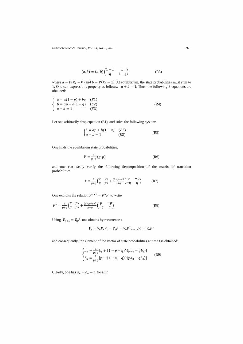
( ) ( ) (
) (R3)
where ( ) and ( ) At equilibrium, the state probabilities must sum to
1. One can express this property as follows: Thus, the following 3 equations are
obtained:
{
( ) ( )
( ) ( ) ( )
(R4)
Let one arbitrarily drop equation (E1), and solve the following system:
{ ( ) ( ) ( )
(R5)
One finds the equilibrium state probabilities:
( ) (R6)
and one can easily verify the following decomposition of the matrix of transition
probabilities:
P =
( )
( )
( ) (R7)
One exploits the relation to write
( )
( )
( ) (R8)
Using one obtains by recurrence :
and consequently, the element of the vector of state probabilities at time t is obtained:
{
[ ( ) ( )]
[ ( ) ( )]
(R9)
Clearly, one has for all n.
Lebanese Science Journal, Vol. 14, No. 2, 2013 98
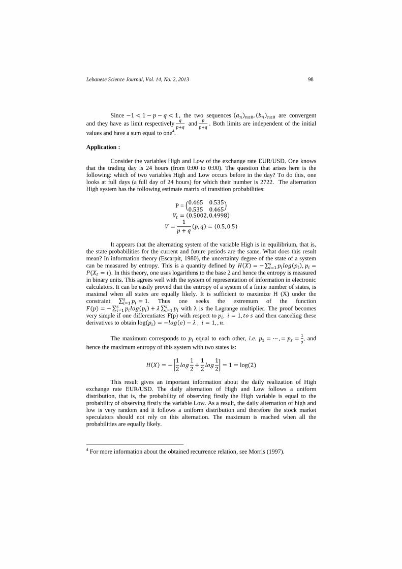
Since , the two sequences ( ) ( ) are convergent
and they have as limit respectively
and
. Both limits are independent of the initial
values and have a sum equal to one4.
Application :
Consider the variables High and Low of the exchange rate EUR/USD. One knows
that the trading day is 24 hours (from 0:00 to 0:00). The question that arises here is the
following: which of two variables High and Low occurs before in the day? To do this, one
looks at full days (a full day of 24 hours) for which their number is 2722. The alternation
High system has the following estimate matrix of transition probabilities:
P = (
)
( )
( ) ( )
It appears that the alternating system of the variable High is in equilibrium, that is,
the state probabilities for the current and future periods are the same. What does this result
mean? In information theory (Escarpit, 1980), the uncertainty degree of the state of a system
can be measured by entropy. This is a quantity defined by ( ) ∑ ( ) ,
( ). In this theory, one uses logarithms to the base 2 and hence the entropy is measured
in binary units. This agrees well with the system of representation of information in electronic
calculators. It can be easily proved that the entropy of a system of a finite number of states, is
maximal when all states are equally likely. It is sufficient to maximize H (X) under the
constraint ∑ . Thus one seeks the extremum of the function
( ) ∑ ( ) ∑
with λ is the Lagrange multiplier. The proof becomes
very simple if one differentiates F(p) with respect to and then canceling these
derivatives to obtain ( ) ( ) .
The maximum corresponds to equal to each other, i.e.
, and
hence the maximum entropy of this system with two states is:
( ) [
] ( )
This result gives an important information about the daily realization of High
exchange rate EUR/USD. The daily alternation of High and Low follows a uniform
distribution, that is, the probability of observing firstly the High variable is equal to the
probability of observing firstly the variable Low. As a result, the daily alternation of high and
low is very random and it follows a uniform distribution and therefore the stock market
speculators should not rely on this alternation. The maximum is reached when all the
probabilities are equally likely.
4 For more information about the obtained recurrence relation, see Morris (1997).

Lebanese Science Journal, Vol. 14, No. 2, 2013 99
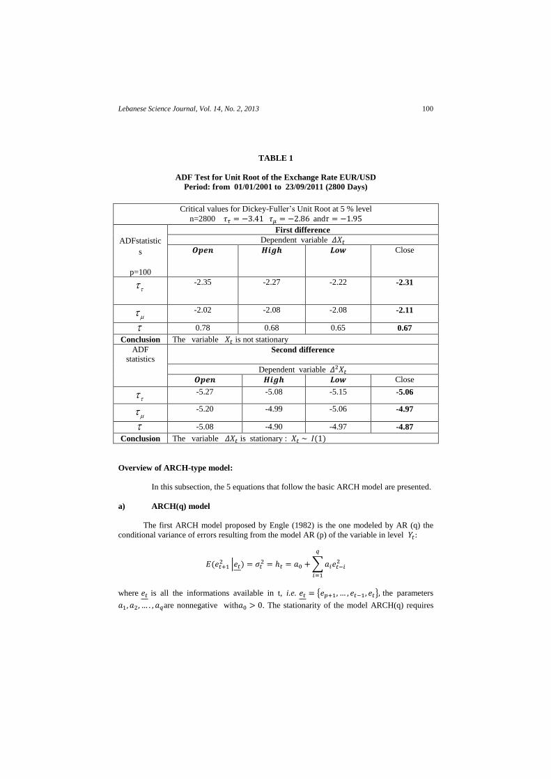
UNIT ROOT TESTS
In times series analysis, it is important to test for whether the variables contain unit
roots. It is widely recognized in the literature that a testing strategy is needed when testing for
a unit root. Fuller (1976), Dickey and Fuller (1981), Perron (1988), Dolado et al. (1990),
Enders (1995), and Ayat and Burridge (2000) propose such strategies:
∑ (M)
where t is the time, and is the variable in first difference, p is the order AR model such
that the associated residues behave like a white noise. Indeed, the non stationarity of a time
series may be due to a linear trend (Trend stationary (TS)) or because of the variance which is
related to the time and consequently the corresponding time series requires a difference at
order (d) to become stationary (it is denoted I (d)), and in a such situation, the process is
called (DS) (difference stationary). The Dickey-Fuller (ADF) procedure proposed by Dickey-
Fuller is actually the most widely used. This procedure leads to decide about the type of non
stationarity (TS or DS). For a variable , the (ADF) procedure distinguishes among three
cases:
a) The equation (M) contains a constant and a trend.
b) The equation (M) contains a constant and without any trend.
c) The equation contains neither a constant nor a trend.
For cases (a), (b) and (c), the ADF procedure suggests respectively the test statistics
called ( ) ( ) ( ). In practice, one estimates the equation (M) and one is interested in
the t statistic . The test statistic is the familiar t statistic but with special critical values
employed to reflect its non normal (even asymptotically) distribution under the null of a unit
root (Elder and Kennedy, 2001). In the following, one will use the ADF procedure using the
RATS software (version 8.2) and one considers the file (F2) which covers data for the period
01/01/2001 - 23/09/2011 (2800 days). The order of the AR (p) model is properly selected to
ensure the presence of residues that behave like a white noise. It seems that p = 100 is an
appropriate value with this type of data. Indeed, 100 days are 4 months of the stock market, so
this is a considerable past to predict the future. The results of unit root test shows that the first
difference must be performed to ensure the stationarity of each of these variables. The results
of the unit root tests are presented in Table (1). All variables are integrated at order one and
this result is necessary to be able to use the two-step cointegration procedure suggested by
Engle and Granger (1987).
MEASURE OF VOLATILITY IN THE EXCHANGE RATE EUR / USD
Instead of considering an ad hoc variable and / or perform a data transformation
(log or other), Engle (1982) showed the possibility of simultaneously modeling the mean and
variance of a time series. Engle methodology indicates that the conditional forecasts are more
effective than the unconditional forecasts. Indeed, the unconditional prediction has an error
prediction variance larger than that obtained in the case of conditional prediction. A simple
strategy can be employed to predict the conditional variance as an AR (q) model. Assume that
the variable is integrated of order d ( ( )), that is , stationary and it follows an
AR (p) model where the are the residues. In the following, the models derived from the
ARCH model, which are widely used in the financial market are briefly presented.
Lebanese Science Journal, Vol. 14, No. 2, 2013 100
TABLE 1
ADF Test for Unit Root of the Exchange Rate EUR/USD
Period: from 01/01/2001 to 23/09/2011 (2800 Days)
Overview of ARCH-type model:
In this subsection, the 5 equations that follow the basic ARCH model are presented.
a) ARCH(q) model
The first ARCH model proposed by Engle (1982) is the one modeled by AR (q) the
conditional variance of errors resulting from the model AR (p) of the variable in level
( | )
∑
where is all the informations available in t, i.e. { } the parameters
are nonnegative with . The stationarity of the model ARCH(q) requires
Critical values for Dickey-Fuller’s Unit Root at 5 % level
n=2800 and
ADFstatistic
s
p=100
First difference
Dependent variable Close
-2.35 -2.27 -2.22 -2.31
-2.02 -2.08 -2.08 -2.11
0.78 0.68 0.65 0.67
Conclusion The variable is not stationary
ADF statistics
Second difference
Dependent variable Close
-5.27 -5.08 -5.15 -5.06
-5.20 -4.99 -5.06 -4.97
-5.08 -4.90 -4.97 -4.87
Conclusion The variable is stationary : ( )
Lebanese Science Journal, Vol. 14, No. 2, 2013 101
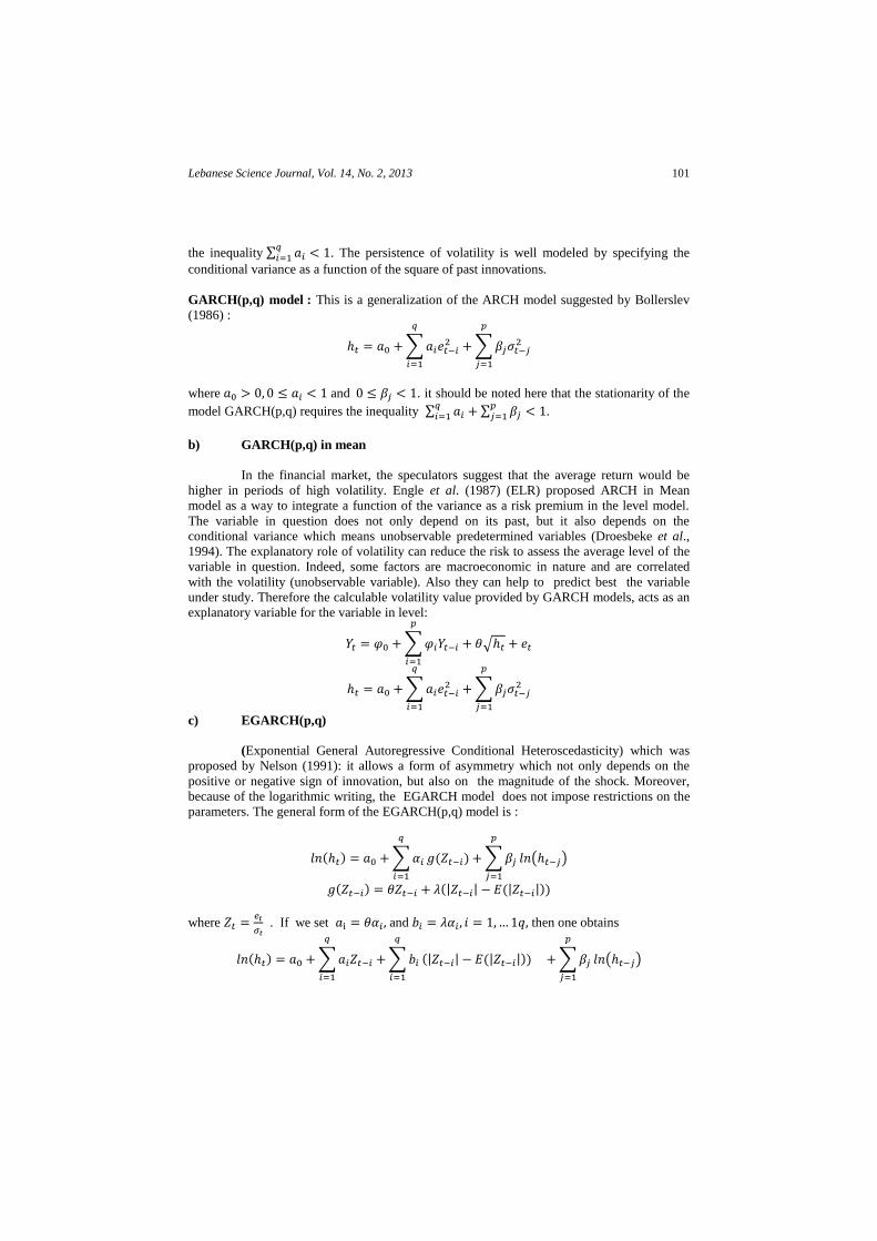
the inequality ∑ . The persistence of volatility is well modeled by specifying the
conditional variance as a function of the square of past innovations.
GARCH(p,q) model : This is a generalization of the ARCH model suggested by Bollerslev
(1986) :
∑ ∑
where and . it should be noted here that the stationarity of the
model GARCH(p,q) requires the inequality ∑ ∑
.
b) GARCH(p,q) in mean
In the financial market, the speculators suggest that the average return would be
higher in periods of high volatility. Engle et al. (1987) (ELR) proposed ARCH in Mean
model as a way to integrate a function of the variance as a risk premium in the level model.
The variable in question does not only depend on its past, but it also depends on the
conditional variance which means unobservable predetermined variables (Droesbeke et al.,
1994). The explanatory role of volatility can reduce the risk to assess the average level of the
variable in question. Indeed, some factors are macroeconomic in nature and are correlated
with the volatility (unobservable variable). Also they can help to predict best the variable
under study. Therefore the calculable volatility value provided by GARCH models, acts as an
explanatory variable for the variable in level:
∑
√
∑ ∑
c) EGARCH(p,q)
(Exponential General Autoregressive Conditional Heteroscedasticity) which was
proposed by Nelson (1991): it allows a form of asymmetry which not only depends on the
positive or negative sign of innovation, but also on the magnitude of the shock. Moreover,
because of the logarithmic writing, the EGARCH model does not impose restrictions on the
parameters. The general form of the EGARCH(p,q) model is :
( ) ∑
( ) ∑
( )
( ) (| | (| |))
where
. If we set and then one obtains
( ) ∑
∑
(| | (| |)) ∑
( )
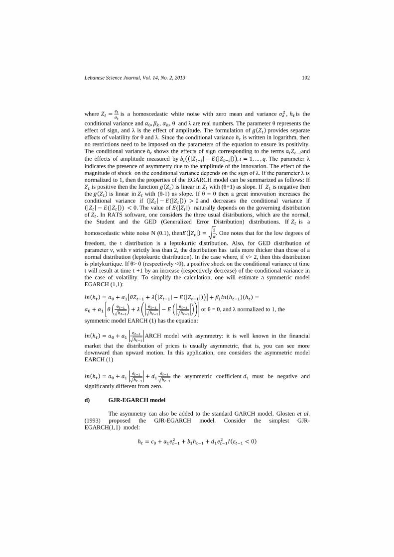
Lebanese Science Journal, Vol. 14, No. 2, 2013 102
where
is a homoscedastic white noise with zero mean and variance
, is the
conditional variance and , , θ and λ are real numbers. The parameter θ represents the
effect of sign, and λ is the effect of amplitude. The formulation of ( ) provides separate
effects of volatility for θ and λ. Since the conditional variance is written in logarithm, then
no restrictions need to be imposed on the parameters of the equation to ensure its positivity.
The conditional variance shows the effects of sign corresponding to the terms and
the effects of amplitude measured by ((| | (| |)) The parameter λ
indicates the presence of asymmetry due to the amplitude of the innovation. The effect of the
magnitude of shock on the conditional variance depends on the sign of λ. If the parameter λ is
normalized to 1, then the properties of the EGARCH model can be summarized as follows: If
is positive then the function ( ) is linear in with (θ+1) as slope. If is negative then
the ( ) is linear in with (θ-1) as slope. If θ = 0 then a great innovation increases the
conditional variance if (| | (| |)) and decreases the conditional variance if (| | (| |)) The value of (| |) naturally depends on the governing distribution
of . In RATS software, one considers the three usual distributions, which are the normal,
the Student and the GED (Generalized Error Distribution) distributions. If is a
homoscedastic white noise N (0.1), then (| |) √
. One notes that for the low degrees of
freedom, the t distribution is a leptokurtic distribution. Also, for GED distribution of
parameter ν, with ν strictly less than 2, the distribution has tails more thicker than those of a
normal distribution (leptokurtic distribution). In the case where, if v> 2, then this distribution
is platykurtique. If θ> 0 (respectively <0), a positive shock on the conditional variance at time
t will result at time t +1 by an increase (respectively decrease) of the conditional variance in
the case of volatility. To simplify the calculation, one will estimate a symmetric model
EGARCH (1,1):
( ) [ (| | (| |))] ( )( )
[ (
√ ) (|
√ | (|
√ |))] or θ = 0, and λ normalized to 1, the
symmetric model EARCH (1) has the equation:
( ) |
√ |ARCH model with asymmetry: it is well known in the financial
market that the distribution of prices is usually asymmetric, that is, you can see more
downward than upward motion. In this application, one considers the asymmetric model
EARCH (1)
( ) |
√ |
√ the asymmetric coefficient must be negative and
significantly different from zero.
d) GJR-EGARCH model
The asymmetry can also be added to the standard GARCH model. Glosten et al.
(1993) proposed the GJR-EGARCH model. Consider the simplest GJR-
EGARCH(1,1) model:
( )
Lebanese Science Journal, Vol. 14, No. 2, 2013 103
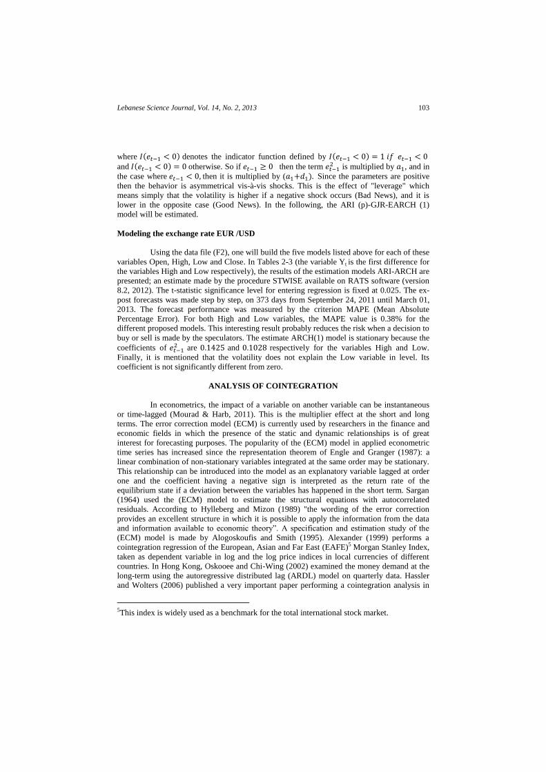
where ( ) denotes the indicator function defined by ( ) and ( ) otherwise. So if then the term
is multiplied by , and in
the case where then it is multiplied by ( ) Since the parameters are positive
then the behavior is asymmetrical vis-à-vis shocks. This is the effect of "leverage" which
means simply that the volatility is higher if a negative shock occurs (Bad News), and it is
lower in the opposite case (Good News). In the following, the ARI (p)-GJR-EARCH (1)
model will be estimated.
Modeling the exchange rate EUR /USD
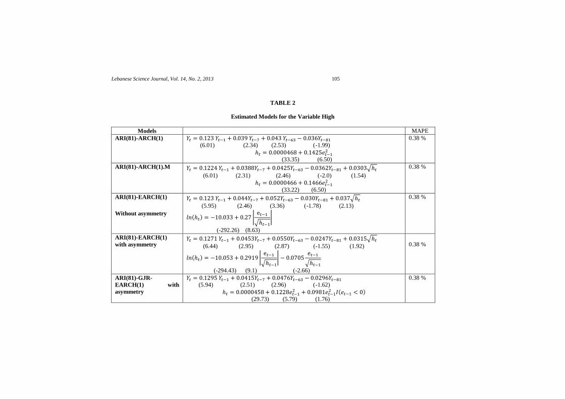
Using the data file (F2), one will build the five models listed above for each of these
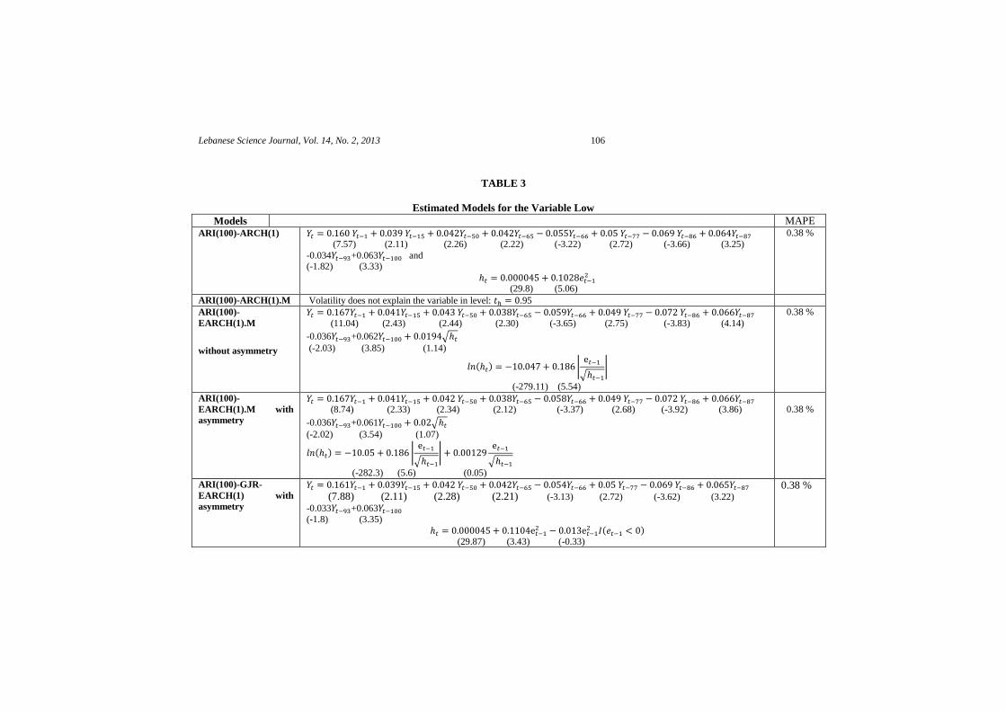
variables Open, High, Low and Close. In Tables 2-3 (the variable Yt is the first difference for
the variables High and Low respectively), the results of the estimation models ARI-ARCH are
presented; an estimate made by the procedure STWISE available on RATS software (version
8.2, 2012). The t-statistic significance level for entering regression is fixed at 0.025. The ex-
post forecasts was made step by step, on 373 days from September 24, 2011 until March 01,
2013. The forecast performance was measured by the criterion MAPE (Mean Absolute
Percentage Error). For both High and Low variables, the MAPE value is 0.38% for the
different proposed models. This interesting result probably reduces the risk when a decision to
buy or sell is made by the speculators. The estimate ARCH(1) model is stationary because the
coefficients of are and respectively for the variables High and Low.
Finally, it is mentioned that the volatility does not explain the Low variable in level. Its
coefficient is not significantly different from zero.
ANALYSIS OF COINTEGRATION
In econometrics, the impact of a variable on another variable can be instantaneous
or time-lagged (Mourad & Harb, 2011). This is the multiplier effect at the short and long
terms. The error correction model (ECM) is currently used by researchers in the finance and
economic fields in which the presence of the static and dynamic relationships is of great
interest for forecasting purposes. The popularity of the (ECM) model in applied econometric
time series has increased since the representation theorem of Engle and Granger (1987): a
linear combination of non-stationary variables integrated at the same order may be stationary.
This relationship can be introduced into the model as an explanatory variable lagged at order
one and the coefficient having a negative sign is interpreted as the return rate of the
equilibrium state if a deviation between the variables has happened in the short term. Sargan
(1964) used the (ECM) model to estimate the structural equations with autocorrelated
residuals. According to Hylleberg and Mizon (1989) "the wording of the error correction
provides an excellent structure in which it is possible to apply the information from the data
and information available to economic theory”. A specification and estimation study of the
(ECM) model is made by Alogoskoufis and Smith (1995). Alexander (1999) performs a
cointegration regression of the European, Asian and Far East (EAFE)5 Morgan Stanley Index,
taken as dependent variable in log and the log price indices in local currencies of different
countries. In Hong Kong, Oskooee and Chi-Wing (2002) examined the money demand at the
long-term using the autoregressive distributed lag (ARDL) model on quarterly data. Hassler
and Wolters (2006) published a very important paper performing a cointegration analysis in
5This index is widely used as a benchmark for the total international stock market.

Lebanese Science Journal, Vol. 14, No. 2, 2013 104
the (ARDL) structure. They showed that the estimation of a cointegrated vector from an
(ARDL) specification is equivalent to the (ECM) model. Using the procedure of Johansen
(1988), Johansen and Juselius (1990), Johansen (1995) in studying the flow of the foreign
direct investment, Mourad and Farhat (2007) found a long-run equilibrium relationship
between the long-term developed countries and the rest of the world. A paper published by
Shahbaz et al. (2008) suggested the existence of a strong relationship between stock market
development and economic growth in Pakistan. A very recent paper (Mourad, 2012) deals
with the private sector deposits in commercial banks in Lebanon. Using the procedure for
cointegration described by Pesaran et al. (2001), the author shows that the residents' deposits
in Lebanese pounds and the foreign currency deposits are linked by a low speed alignment to
the long - run equilibrium when shocks occur in the short term. Using the Johansen
procedure, Bangoura (2012) shows that there is a cointegration relationship between the
variables of economic growth and financial development (GDP, domestic credit banking,
domestic private sectors, and inflation) for the 11 CEDEAO countries and 7 UEMOA
countries6.
In the following, the two-step procedure of cointegration proposed by Engle and
Granger (1987) will be used. Indeed, since there are a long size series in which the
autoregressive models (AR) have a higher orders (p ) and since in these estimated
models, there are many parameters that are not significantly different from zero, the use of the
Johansen-Juselius procedure to estimate the vector of the error correction model (VECM)
with all parameters will lead to highly charged models with a mixing of significant and
insignificant parameters. On the other hand, in these systems, especially the first two systems,
the Open variable is observed at time ( ), where T is the present time. Indeed, it is the
time of opening market at midnight in the Middle East countries and consequently, the value
of the Open variable will participate better in the forecasting of the variables High and Low.
For stock market speculators, the forecast for high and low is very important because any
decision concerning buying or selling depends on it. In the following, one will discuss the
four following systems7:
System 1: It involves the two variables Open and High.
System 2: It involves the two variables Open and Low.
System 3: It involves the three variables Open, Low and High.
System 4: It is concerned with the four variables Open, Low, Close and High.
The number of parameters m in any long-term equilibrium relationship of the
system (i), i = 1, 2, 3, 4 are respectively 2, 2, 3 and 4. Next, the first 2800 observations of the
data file (F2) are used to estimate the four systems, then one performs a calculation of ex-post
forecasts for the 373 days starting from September 24, 2011 until March 01, 2013.
To test the static cointegration between the variables of a system, the two-step
procedure proposed by Engle and Granger (1987) will be used:
Step 1: One identifies the order of integration (d) for each variable.
6Communauté Économique des États de l’Afrique de l’Ouest (CEDEAO) et Union
Économique et Monétaire Ouest-Africaine (UEMOA). 7A system is a model that explores the dynamic relationship between two or more variables.
Lebanese Science Journal, Vol. 14, No. 2, 2013 105
TABLE 2
Estimated Models for the Variable High
Models MAPE
ARI(81)-ARCH(1)
(6.01) (2.34) (2.53) (-1.99)
(33.35) (6.50)
0.38 %
ARI(81)-ARCH(1).M √ (6.01) (2.31) (2.46) (-2.0) (1.54)
(33.22) (6.50)
0.38 %
ARI(81)-EARCH(1)
Without asymmetry
√ (5.95) (2.46) (3.36) (-1.78) (2.13)
( ) |
√ |
(-292.26) (8.63)
0.38 %
ARI(81)-EARCH(1)
with asymmetry √ (6.44) (2.95) (2.87) (-1.55) (1.92)
( ) |
√ |
√
(-294.43) (9.1) (-2.66)
0.38 %
ARI(81)-GJR-
EARCH(1) with
asymmetry
(5.94) (2.51) (2.96) (-1.62)
( ) (29.73) (5.79) (1.76)
0.38 %
Lebanese Science Journal, Vol. 14, No. 2, 2013 106
TABLE 3
Estimated Models for the Variable Low
Models MAPE ARI(100)-ARCH(1)
(7.57) (2.11) (2.26) (2.22) (-3.22) (2.72) (-3.66) (3.25)
-0.034 +0.063 and (-1.82) (3.33)
(29.8) (5.06)
0.38 %
ARI(100)-ARCH(1).M Volatility does not explain the variable in level: .95
ARI(100)-
EARCH(1).M
without asymmetry
(11.04) (2.43) (2.44) (2.30) (-3.65) (2.75) (-3.83) (4.14)
-0.036 +0.062 √ (-2.03) (3.85) (1.14)
( ) |
√ |
(-279.11) (5.54)
0.38 %
ARI(100)-
EARCH(1).M with
asymmetry
(8.74) (2.33) (2.34) (2.12) (-3.37) (2.68) (-3.92) (3.86)
-0.036 +0.061 √ (-2.02) (3.54) (1.07)
( ) |
√ |
√
(-282.3) (5.6) (0.05)
0.38 %
ARI(100)-GJR-
EARCH(1) with
asymmetry
(7.88) (2.11) (2.28) (2.21) (-3.13) (2.72) (-3.62) (3.22) -0.033 +0.063 (-1.8) (3.35)
( ) (29.87) (3.43) (-0.33)
0.38 %
Lebanese Science Journal, Vol. 14, No. 2, 2013 107
Step 2: One estimates the eventual long-run equilibrium relationship among the different
variables of the systems and one covers the residues of this equation. This error term
represents the disequilibrium or cointegrating regression. The stationarity of residues
implies that the variables are cointegrated, and in order to test the stationarity of , the
appropriate ADF equation are used. Indeed, the residuals have a mean of zero and hence it is
not necessary to inspect the presence of a linear trend. One may also use the usual statistical
Durbin and Watson (DW) under certain conditions (Mourad, 2007). To test the existence of a
unit root in the residuals associated to the static relationship, one proceeds as follows:
∑ (E)
∑ (E)
It is worth mentioning here that the order m is determined by using the Ljung-Box
Q-statistic for the residuals of the model (M). In the present case, for each system, each
component is ( ) and consequently all variables are integrated at the same order.Using the
data file (F2) of size 2800, one tests whether the disequilibrium error is I(0). For this,
is compared to critical value for a 5 % level of significance tabulated by Mackinnon (1991).
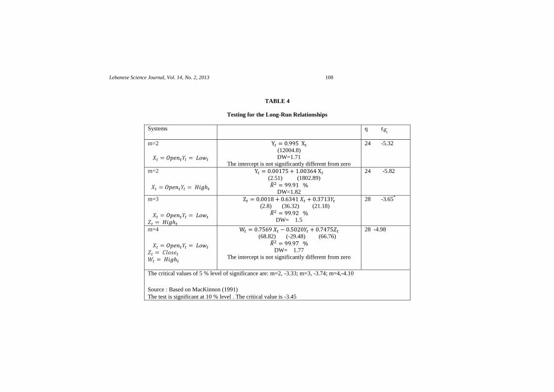
The results of the testing for the long-run relationships are given in Table (4). For all systems,
the cointegrating regression is accepted. Therefore, a variation in the dependent variable (per
example, in system 1, in system 2) depends on the variation in the variable
where the different lags are given in Table (5) and in the magnitude of the departure
from the long-run relationship at the previous period. The negative coefficients of , -
0.3339, -0.4125, -0.298 and -0.099 respectively in the systems 1, 2, 3 and 4, represent the
adjustment speed that leads to validate the ECM model and there will be a return of the
dependent variable to its equilibrium in the long-run. Finally, the ECM for all systems is
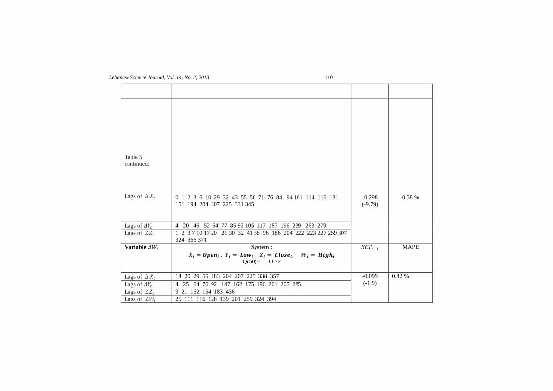
estimated. In Table (5), one deals only with the lagged corresponding parameters, which are
significantly different from zero.
For each system, a prediction step by step (ex-post forecasts) covering the period
from September 24, 2011 until March 01, 2013, that is 373 days is performed. The forecasting
performance is measured by the MAPE criterion (see Table 5). The inspection of the results
reveals the importance of the proposed models especially for the first two systems 1 and 2.
Indeed, the value of MAPE is 0.3%, an excellent result was found among all models.These
results are of great interest to measure risk in the exchange rate EUR / USD. Therefore, if a
shock in the high, for example, produces a deviation from the target balance, a restoring force
of 33.39 % will be generated to correct it the next day. This deviation, within three days, the
variable High returns to its long-term target. The same conclusion goes for the variable Low,
but with faster restoring force (41.25 %). The advice could be granted to persons interested in
the exchange rate EUR / USD because it accentuates the confidence of the speculators of the
stock market in this efficient forecasting results.
Lebanese Science Journal, Vol. 14, No. 2, 2013 108
TABLE 4
Testing for the Long-Run Relationships
Systems q
m=2
(12004.8)
DW=1.71
The intercept is not significantly different from zero
24 -5.32
m=2
(2.51) (1802.89)
DW=1.82
24 -5.82
m=3
(2.8) (36.32) (21.18)
DW= 1.5
28 -3.65*
m=4
(68.82) (-29.48) (66.76)
DW= 1.77
The intercept is not significantly different from zero
28 -4.98
The critical values of 5 % level of significance are: m=2, -3.33; m=3, -3.74; m=4,-4.10
Source : Based on MacKinnon (1991)
The test is significant at 10 % level . The critical value is -3.45
Lebanese Science Journal, Vol. 14, No. 2, 2013 109
TABLE 5
The Estimate Error Correction Models and Forecasts
Variable System : Q(50) = 55.41
Q represents the Ljung-Box statistics
MAPE
Lags of Δ
0 1 2 3 14 23 24 45 63 87 113 114 141 153 163 182 197 220
236 238 256 262284 297 326 328 331 369
-0.3339
(-7.83)
0.30 %
Lags of 1 2 3 10 24 43 55 81 92 112 116 128
130 155 175 231 259 303 399
Variable System : Q(50) = 63.46
MAPE
Lags of Δ
0 1 2 3 4 6 20 29 55 56 63 71 73 76 77 80 85 92 101 114
116 125 151 183 185 203 204 205 207 218 239 260 262 306
339
-0.4125
(-9.94)
0.30 %
Lags of 1 2 3 4 7 10 13 17 21 41 47 52 58 96 131 139 164 194 222
227 255 259 279 307 324 366 376
Variable System : Q(50)= 57.46
MAPE
Lebanese Science Journal, Vol. 14, No. 2, 2013 110
Table 5 continued:
Lags of Δ
0 1 2 3 6 10 29 32 43 55 56 71 76 84 94 101 114 116 131
151 194 204 207 225 331 345
-0.298
(-9.79)
0.38 %
Lags of 4 20 46 52 64 77 85 92 105 117 187 196 239 263 279
Lags of 1 2 3 7 10 17 20 21 30 32 41 58 96 186 204 222 223 227 259 307
324 366 371
Variable System :
Q(50)= 33.72
MAPE
Lags of Δ 14 20 29 55 183 204 207 225 338 357 -0.099
(-1.9)
0.42 %
Lags of 4 25 64 76 92 147 162 175 196 201 205 285
Lags of 9 21 152 154 183 436
Lags of 25 111 116 128 139 201 259 324 394
Lebanese Science Journal, Vol. 14, No. 2, 2013 111
CONCLUSION
In this paper, 4 main points will be beneficial for those who supervise the evolution of
the exchange rate EUR / USD. The first point shows that the alternation of High and Low on the
market follows a uniform distribution and hence if someone bets on this alternation then he puts
himself in a position of maximum uncertainty. The second point is related to the daily volatility
of High and Low. These variables require a first difference to become stationary and the
residuals associated to the integrated autoregressive models have an ARCH effect. The five
proposed models associated to the variables in first differences and volatility have the same
predictive performance (MAPE = 0.38%). It seems that the statistical quality of the models
AR(81).M-EARCH (1) without asymmetry and ARI (81).M-EARCH (1) is better for High
variable, while for the variable Low, ARI (100)-ARCH (1) and ARI (100)-EARCH (1).M
without asymmetry seem the best models. The latter point seems the more interesting one. In
fact, the components of each of the four systems are cointegrated. More precisely, the
components of each system (High, Open) and (Low, Open) are linked by a long-run equilibrium
relationship. In addition, the error correction mechanism is very fast, 33.39% for the Low
variable and 41.25 % for the High variable. Also, a return to equilibrium occurs between two
and three days, and the short-term forecasts for High and Low variables are very close to the
reality (MAPE = 0.3%). As a conclusion, the (ECM) models led to a 21% improvement in
prediction accuracy when compared to the ARI-ARCH models.
RECOMMENDATIONS
At the end of this research, a large question arises: can one determine the probability
of the predicted values of the two variables High and Low? These probabilities could be
empirically estimated using the proposed models for each of the two variables provided if the
parameters stability is validated by an adequate test as the Chow test for parameter stability or
the recursive Chow test.
REFERENCES
Alexander, C. 1999. Optimal hedging using cointegration. Philosophical Transactions of the
Royal Society, London, series A 357, pp 2039-2058.
Allegret, J-P. 2007. Which currency exchange regime for emerging Markets? Corner Solutions
under question. Panoeconomicus, 54(4): 397-427.
Alogoskoufis, G., Smith, R. 1995. On error correction models: specification, interpretation,
estimation. In Surveys in Econometrics (L. Oxley, D.A.R. George, C.J. Roberts, S.
Sayer, eds.), pp 139-170. Blackwell Publishers, Oxford.
Ayat, L., and Burridge, P. 2000. Unit root tests in the presence of uncertainty about the non-
stochastic trend. Journal of Econometrics, 95(1): 71–96.
Bollerslev, T. 1986. Generalized autoregressive conditional heteroskedasticity. Journal of
Econometrics, 31: 307-327.
Bénassy-Quéré, A., Béreau, S. et Mignon, V. 2009. Taux de change d’équilibre. Une question
d’horizon. Revue Économique, 60: 657-666.
Bangoura, L. 2012. Cointégration et causalité entre croissance économique et développement
financier: pays de la Cedeao et de l’Emoa. International Research Journal of Finance
and Economics (IRJFE), 91: 78-97.
Dickey, D.A. and Fuller, W.A. 1981. Likelihood ratio statistics for autoregressive time series
with a unit root. Econometrica, 49(4): 1057–72.

Lebanese Science Journal, Vol. 14, No. 2, 2013 112
Dolado, J., Jenkinson, T. and Sosvilla-Rivero, S. 1990. Cointegration and unit roots. Journal of
Economic Surveys, 4(3): 249–73.
Droesbeke, J.J., Fichet, B. and Tassi P. 1994. Modélisation ARCH : théorie statistique et
application dans le domaine de la finance. Ellipses, Bruxelles, Belgique.
Dunis, C.L., Laws, J. and Sermpinis, G. 2008. Modelling and trading the EUR/USD exchange
rate at the ECB fixing. Liverpool Business School, CIBEF, Liverpool John Moores
University, working paper.
Elder, J. and Kennedy, P.E. 2001. Testing for unit roots: what should students be taught?
Journal of Economic Education, 32: 137–146.
Engle, R.F. 1982. Autoregressive conditional heteroscedasticity with estimates of the variance
of United Kingdom inflation. Econometrica, 50: 987-1007.
Engle, R.F., Lilien, D.M., Robins, R.P. 1987. Estimating time varying risk premia in the term
structure: the Arch-M model. Econometrica, 55(2): 391-407.
Engle, R.F. and Granger, C.W.J. 1987. Co-integration and error correction: representation,
estimation, and testing. Econometrica, 55(2): 251-276.
Enders, W. 1995. Applied econometric time series. New York, Wiley.
Escarpit, R. 1980. Théorie générale de l’information et de la communication. Edition Hachette,
Paris, France.
Fuller, W.A. 1976. Introduction to statistical time series. New York, John Wiley.
Glosten, L.R., Jagannathan, R., Runkle, D.E. 1993. On the relation between the expected value
and the volatility of the nominal excess return on stocks. The Journal of Finance,
XLIII(5): 1779-1801.
Hassler, U. and Wolters, J. 2006. Autoregressive distributed lag models and cointegration.
Advance in Statistical Analysis (ASTA), 90(1): 59-74.
Hylleberg, S. and Mizon, G.E. 1989. Cointegration and error correction mechanisms. The
Economic Journal, 99: 113-125.
Johansen, S. 1988. Satistical analysis of co-integrated vectors. Journal of Economic Dynamics
and Control, 12: 231-254.
Johansen, S. 1995. Statistical analysis of I(2) variables. Econometric Theory, 11: 25-59.
Johansen, S. and Juselius, K. 1990. Maximum likelihood estimation and inference on
cointegration-with application to the demand for money. Oxford Bulletin of
Economics and Statistics, 52: 169-210.
Mackinnon, J.G. 1991. Critical values for cointegration tests. Oxford University Press.
Morris, J.R. 1997. Markov chains. Cambridge University Press.
Mourad, M. 2007. Modeling the import and export system of the United States : using the error
correction model representation. Dirasat, Administrative Sciences, 34(1): 182-199.
Mourad, M. and Farhat, M. 2007. The foreign direct investment of outflows in the world: a co-
integration analysis. Arab Journal of Administration, 27(2): 217-242.
Mourad, M., Harb, A. 2011. Mesure de la fonction de réponse impulsionnelle dans les modèles
autorégressifs. Journal Scientifique Libanais, 12(2) : 117-132.
Mourad, M. 2012. L’analyse des dépôts du secteur privé dans les banques commerciales au
Liban : application du modèle ARDL. Journal Scientifique Libanais, 13(2): 149-166.
Nelson, D.B. 1991. Conditional heteroskedasticity in asset returns: a new approach.
Econometrica, 59: 347-370.
Oskooee, M.B. and Chi Wing Ng, R. 2002. Long-run demand for money in Hong Kong: an
application of the ARDL model. International Journal of Business and Economics,
1(2): 147-155.
Papoulis, A. 1986. Probability, random variables, and stochastic processes. McGraw-Hill Book
Company.
Lebanese Science Journal, Vol. 14, No. 2, 2013 113
Perron, P. 1988. Trends and random walks in macroeconomic time series. Journal of Economic
Dynamics and Control, 12(12): 297–332.
Pesaran, M.H., Shin, Y. and Smith, R.J. 2001. Bounds testing approaches to the analysis of
level relationships. Journal of Applied Econometrics, 16: 289-326.
Render, B., Ralph, M. and Stair, J.R. 1994. Quantitative analysis for management. Prentice
Hall, Englewood Cliffs, New Jersey.
Sargan, J.D. 1964. Wages and prices in the United Kingdom: a study in econometric
methodology. In: Econometric Analysis for National Economic Planning (R.E. Hart,
G. Mills, J.K. Whittaker, eds.), pp. 25-54, Butterworths, London.
Shahbaz, M., Ahmed, N., Ali, L. 2008. Stock market development and economic growth:
ARDL causality in Pakistan. International Research Journal of Finance and
Economics, 14: 182-195.

Lebanese Science Journal, Vol. 14, No. 2, 2013 114