Introduction to Predictive Modeling Using GLMs

A Practitioner’s Viewpoint

Dan Tevet, FCAS, MAAA

Anand Khare, FCAS, MAAA, CPCU

1

•Overview of predictive modeling

•Predictive modeling in the actuarial world

•Simple linear models vs generalized linear

models (GLMs)

•Specification of GLMs

• Interpretation of GLM output

•Frequency/severity vs pure premium modeling

•Model validation

2

Outline

•Model – an abstraction of reality, generally with a random or probabilistic component

–Simplification of a real world phenomenon

•Model types include:

– Linear models – predict target variable using linear combination of predictor variables

–Trees – split dataset, one variable at a time, into subgroups that behave similarly

–Neural networks – “self-learning” algorithms that adapt to best predict a quantity of interest

3

What is Predictive Modeling

• Rating plans – model insurance loss data to build

plans that charge actuarially fair rates

• Underwriting plans – knowing relative riskiness of

policyholder can inform underwriting decisions

• Enterprise risk management – model correlations

between lines of business or probability of ruin

• Customer retention – model probability of

customer renewing each year

4

How Do Actuaries Use Modeling?

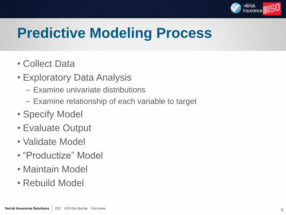
• Collect Data

• Exploratory Data Analysis

– Examine univariate distributions

– Examine relationship of each variable to target

• Specify Model

• Evaluate Output

• Validate Model

• “Productize” Model

• Maintain Model

• Rebuild Model

5

Predictive Modeling Process

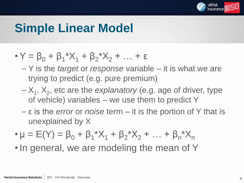
• Y = β0 + β1*X1 + β2*X2 + … + ε

– Y is the target or response variable – it is what we are

trying to predict (e.g. pure premium)

– X1, X2, etc are the explanatory (e.g. age of driver, type

of vehicle) variables – we use them to predict Y

– ε is the error or noise term – it is the portion of Y that is

unexplained by X

• μ = E(Y) = β0 + β1*X1 + β2*X2 + … + βn*Xn

• In general, we are modeling the mean of Y

6

Simple Linear Model

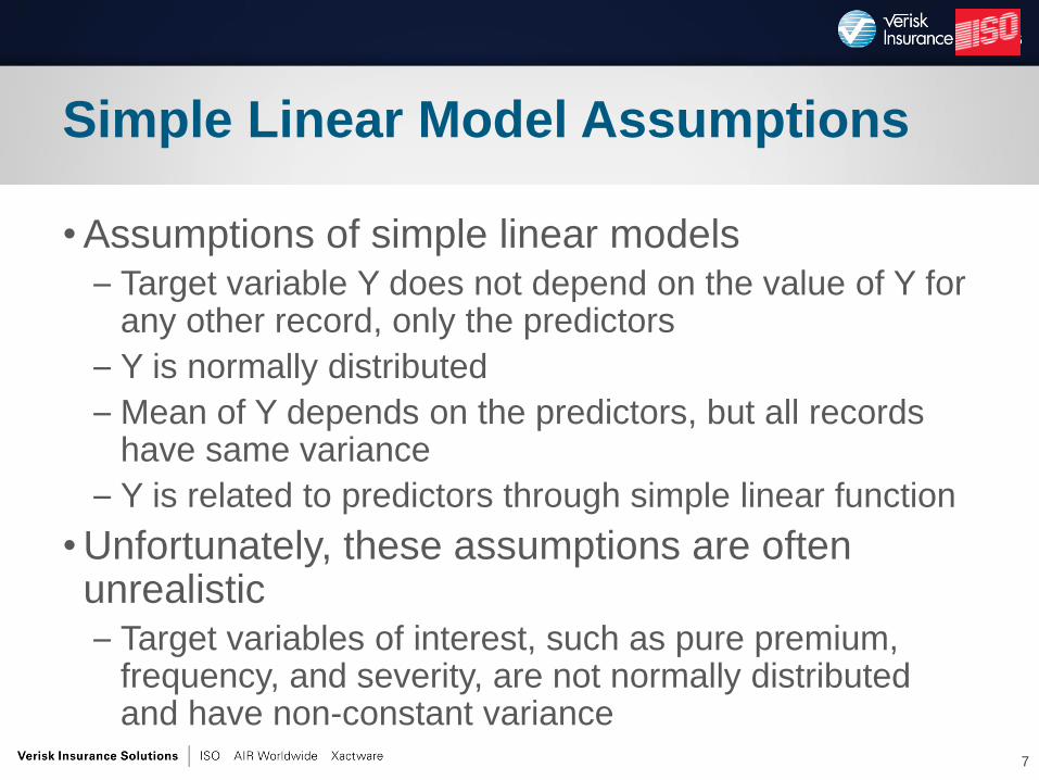
• Assumptions of simple linear models – Target variable Y does not depend on the value of Y for

any other record, only the predictors

– Y is normally distributed

– Mean of Y depends on the predictors, but all records have same variance

– Y is related to predictors through simple linear function

• Unfortunately, these assumptions are often unrealistic – Target variables of interest, such as pure premium,

frequency, and severity, are not normally distributed and have non-constant variance

7

Simple Linear Model Assumptions

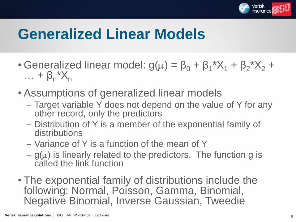
• Generalized linear model: g() = β0 + β1*X1 + β2*X2 + … + βn*Xn

• Assumptions of generalized linear models – Target variable Y does not depend on the value of Y for any

other record, only the predictors

– Distribution of Y is a member of the exponential family of distributions

– Variance of Y is a function of the mean of Y

– g() is linearly related to the predictors. The function g is called the link function

• The exponential family of distributions include the following: Normal, Poisson, Gamma, Binomial, Negative Binomial, Inverse Gaussian, Tweedie

8

Generalized Linear Models

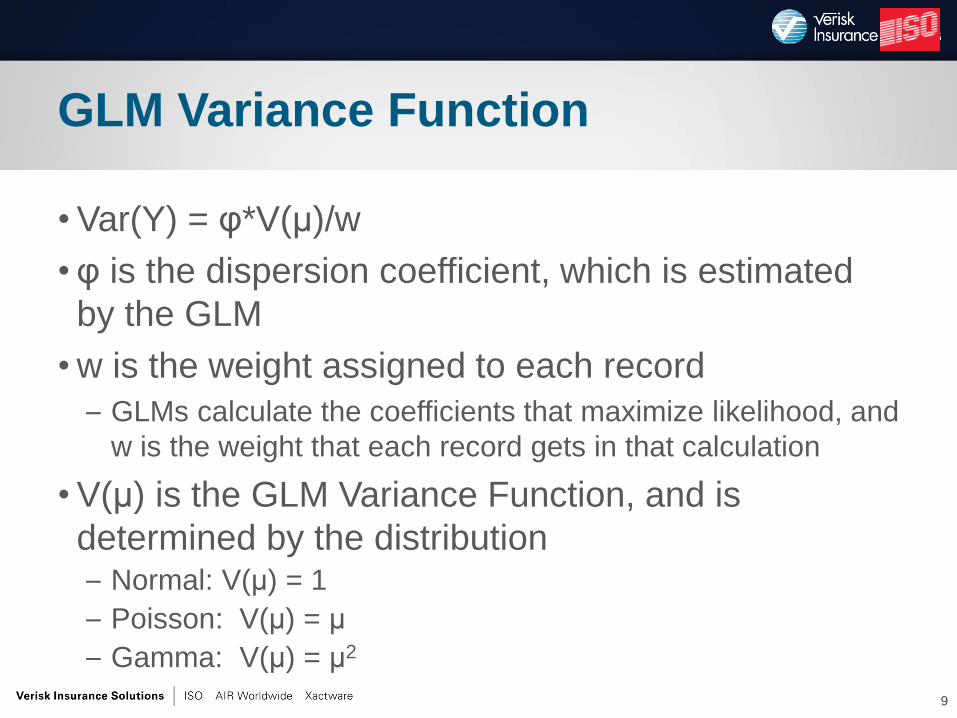
• Var(Y) = φ*V(μ)/w

• φ is the dispersion coefficient, which is estimated

by the GLM

• w is the weight assigned to each record

– GLMs calculate the coefficients that maximize likelihood, and

w is the weight that each record gets in that calculation

• V(μ) is the GLM Variance Function, and is

determined by the distribution – Normal: V(μ) = 1

– Poisson: V(μ) = μ

– Gamma: V(μ) = μ2

9

GLM Variance Function

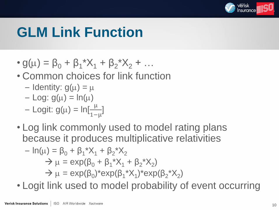
• g() = β0 + β1*X1 + β2*X2 + …

• Common choices for link function – Identity: g() =

– Log: g() = ln()

– Logit: g() = ln[µ

1−µ]

• Log link commonly used to model rating plans because it produces multiplicative relativities – ln() = β0 + β1*X1 + β2*X2

= exp(β0 + β1*X1 + β2*X2)

= exp(β0)*exp(β1*X1)*exp(β2*X2)

• Logit link used to model probability of event occurring

10

GLM Link Function

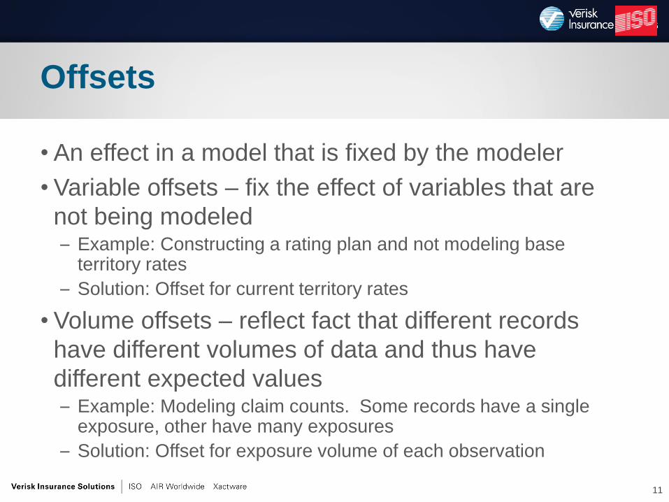
• An effect in a model that is fixed by the modeler

• Variable offsets – fix the effect of variables that are

not being modeled – Example: Constructing a rating plan and not modeling base

territory rates

– Solution: Offset for current territory rates

• Volume offsets – reflect fact that different records

have different volumes of data and thus have

different expected values – Example: Modeling claim counts. Some records have a single

exposure, other have many exposures

– Solution: Offset for exposure volume of each observation

11

Offsets

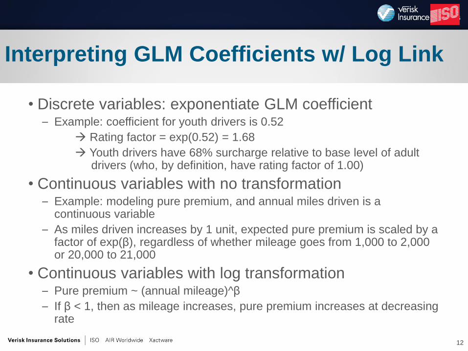
• Discrete variables: exponentiate GLM coefficient – Example: coefficient for youth drivers is 0.52

Rating factor = exp(0.52) = 1.68

Youth drivers have 68% surcharge relative to base level of adult drivers (who, by definition, have rating factor of 1.00)

• Continuous variables with no transformation – Example: modeling pure premium, and annual miles driven is a

continuous variable

– As miles driven increases by 1 unit, expected pure premium is scaled by a factor of exp(β), regardless of whether mileage goes from 1,000 to 2,000 or 20,000 to 21,000

• Continuous variables with log transformation – Pure premium ~ (annual mileage)^β

– If β < 1, then as mileage increases, pure premium increases at decreasing rate

12

Interpreting GLM Coefficients w/ Log Link

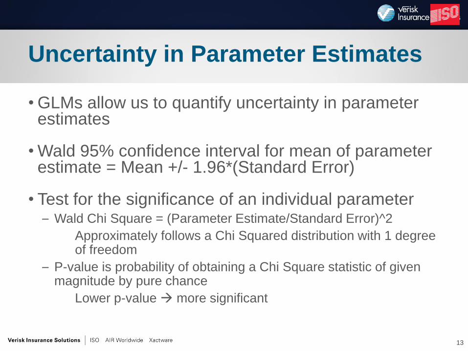
• GLMs allow us to quantify uncertainty in parameter estimates

• Wald 95% confidence interval for mean of parameter estimate = Mean +/- 1.96*(Standard Error)

• Test for the significance of an individual parameter – Wald Chi Square = (Parameter Estimate/Standard Error)^2

Approximately follows a Chi Squared distribution with 1 degree of freedom

– P-value is probability of obtaining a Chi Square statistic of given magnitude by pure chance

Lower p-value more significant

13

Uncertainty in Parameter Estimates

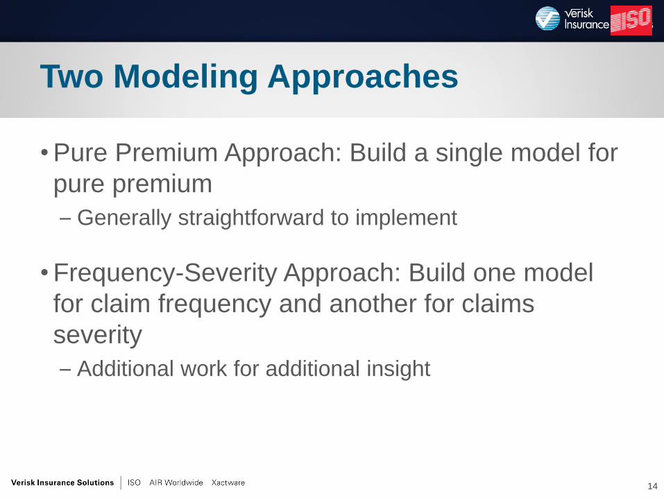
• Pure Premium Approach: Build a single model for

pure premium

– Generally straightforward to implement

• Frequency-Severity Approach: Build one model

for claim frequency and another for claims

severity

– Additional work for additional insight

14

Two Modeling Approaches

• Advantages: – Only a single model needs to be built

– No need to split variable offsets

– Results often very similar to frequency-severity approach

• Disadvantages: – Yields less insight than frequency-severity

– Tweedie distribution is only good choice

• Relatively new and mathematically complex

• Includes implicit assumptions that may not hold

15

Pure Premium Approach

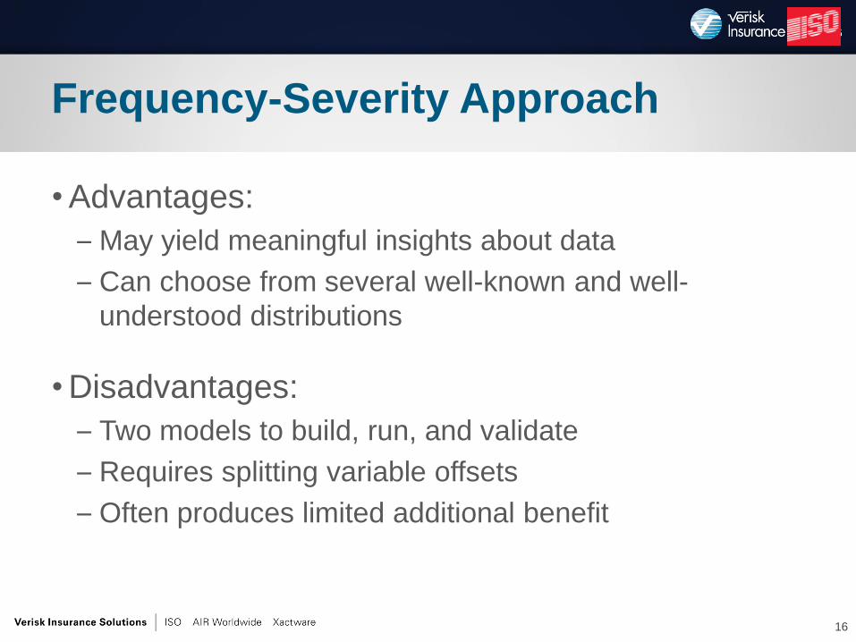
• Advantages:

– May yield meaningful insights about data

– Can choose from several well-known and well-

understood distributions

• Disadvantages:

– Two models to build, run, and validate

– Requires splitting variable offsets

– Often produces limited additional benefit

16

Frequency-Severity Approach

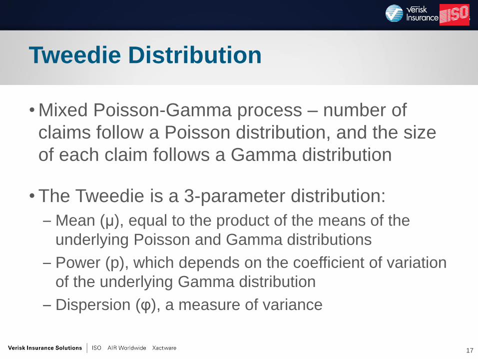
• Mixed Poisson-Gamma process – number of

claims follow a Poisson distribution, and the size

of each claim follows a Gamma distribution

• The Tweedie is a 3-parameter distribution:

– Mean (μ), equal to the product of the means of the

underlying Poisson and Gamma distributions

– Power (p), which depends on the coefficient of variation

of the underlying Gamma distribution

– Dispersion (φ), a measure of variance

17

Tweedie Distribution

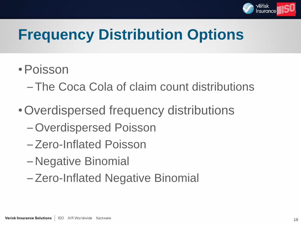
•Poisson

–The Coca Cola of claim count distributions

•Overdispersed frequency distributions

–Overdispersed Poisson

–Zero-Inflated Poisson

–Negative Binomial

–Zero-Inflated Negative Binomial

18

Frequency Distribution Options

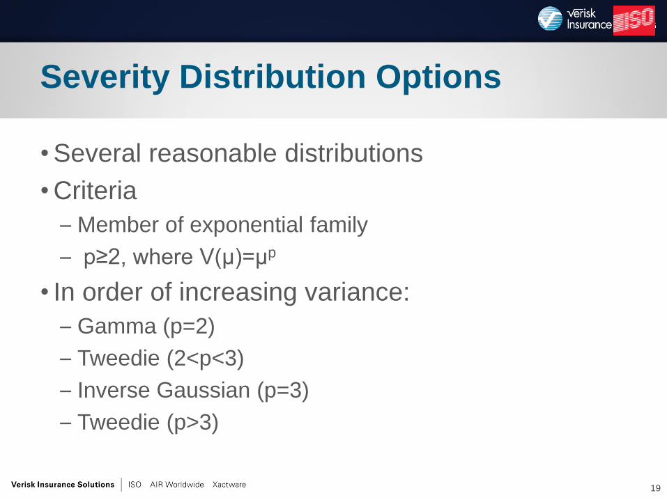
• Several reasonable distributions

• Criteria

– Member of exponential family

– p≥2, where V(µ)=µp

• In order of increasing variance:

– Gamma (p=2)

– Tweedie (2<p<3)

– Inverse Gaussian (p=3)

– Tweedie (p>3)

19

Severity Distribution Options

•Tests of Fit

•Tests of Lift

•Tests of Stability

20

Three Pillars of Model Validation

•Traditional: Absolute/Squared Error

•Alternatives: Likelihood, Deviance, Pearson’s

Chi-Squared

•Penalized: AIC, BIC

•Per Observation: Residuals, Leverage

21

Fit Statistics

• Only appropriate if data is normally distributed

• Inappropriate to use on disaggregate claim

frequency, severity, or pure premium data

• Useful to assess model fit within buckets

– Bucket data into percentiles, or similar quantiles,

and calculate squared difference between actual

and predicted for each bucket

22

Absolute/Squared Error

• Likelihood: chance of observation, given model

– Always increases as parameters are added to model

• Deviance: twice the difference in loglikelihoods

between the saturated and fitted models

– GLMs are fit so as to minimize deviance

– Accounts for the shape of the distribution

• Pearson’s chi-squared: squared error divided by

the variance function of the distribution

– Accounts for the skew of the distribution

23

Better Alternatives to Squared Error

• Akaike Information Criterion (AIC): Penalizes

loglikelihood for additional model parameters

• Bayesian Information Criterion (BIC): Penalizes

loglikelihood for additional model parameters,

and this penalty increases as the number of

records in the dataset increases

– Can be too restrictive

• Used primarily for variable selection

24

Penalized Measures

• Traditional residual: actual minus predicted

• Deviance residual: square root of weighted

deviance times sign of actual minus predicted

– Reflects the shape of the distribution

– Plotting deviance residual against weight or any

predictor should yield an uninformative cloud

– Should be approximately normally distributed

• Leverage: used to identify extreme outliers

– Does not necessarily measure impact

25

Per Observation

• Lift is meant to approximate economic value

– Fit has no relationship with economic value

• Economic value is produced by comparative

advantage in avoidance of adverse selection

– Lift is a comparative measure, i.e. the lift of one model

over another, or the lift of a model over status quo

• Lift should always be measured on holdout data

26

Model Lift

•Simple Quantile Plot

•Double Lift Chart

•Loss Ratio Chart

•Gini Index

27

Lift Measures

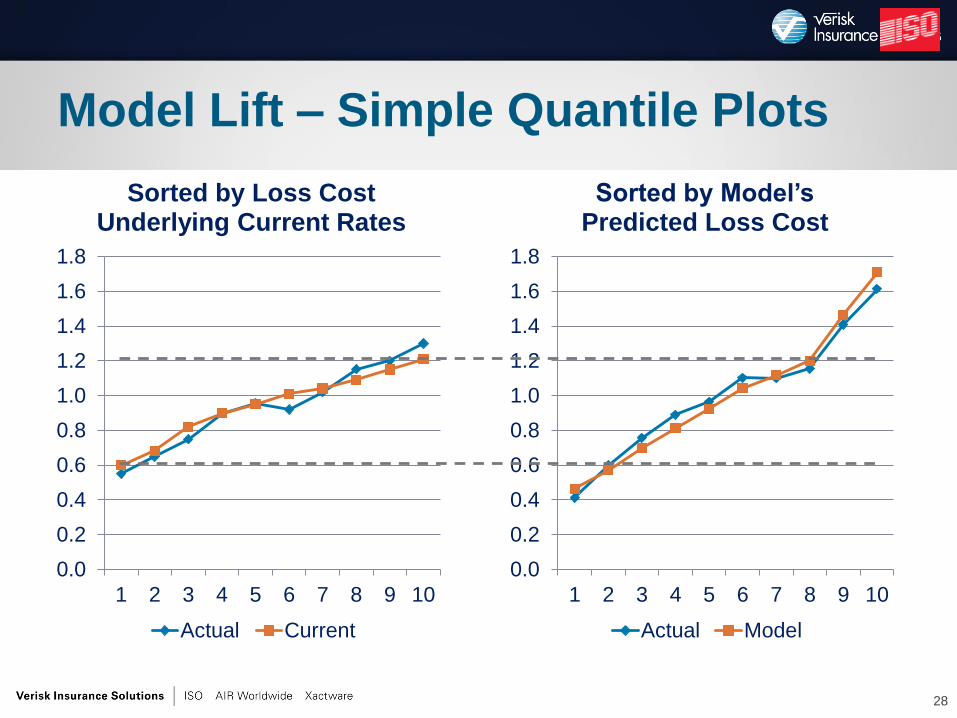
Model Lift – Simple Quantile Plots

28

0.0

0.2

0.4

0.6

0.8

1.0

1.2

1.4

1.6

1.8

1 2 3 4 5 6 7 8 9 10

Sorted by Model’s Predicted Loss Cost

Actual Model

0.0

0.2

0.4

0.6

0.8

1.0

1.2

1.4

1.6

1.8

1 2 3 4 5 6 7 8 9 10

Sorted by Loss Cost Underlying Current Rates

Actual Current

29

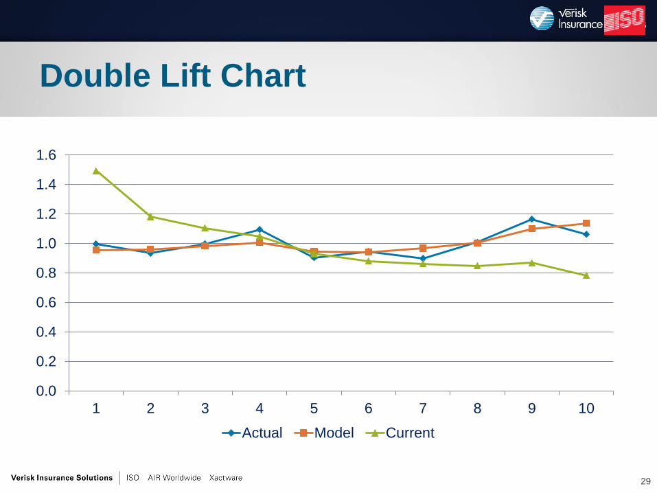
Double Lift Chart

0.0

0.2

0.4

0.6

0.8

1.0

1.2

1.4

1.6

1 2 3 4 5 6 7 8 9 10

Actual Model Current

30

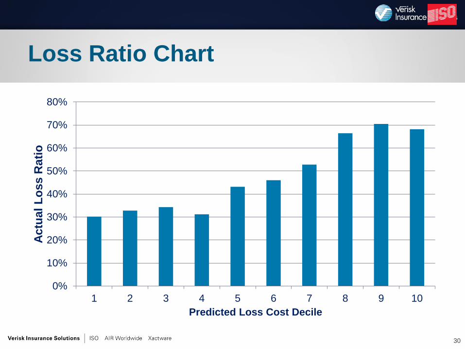
Loss Ratio Chart

0%

10%

20%

30%

40%

50%

60%

70%

80%

1 2 3 4 5 6 7 8 9 10

Actu

al

Lo

ss R

ati

o

Predicted Loss Cost Decile

31

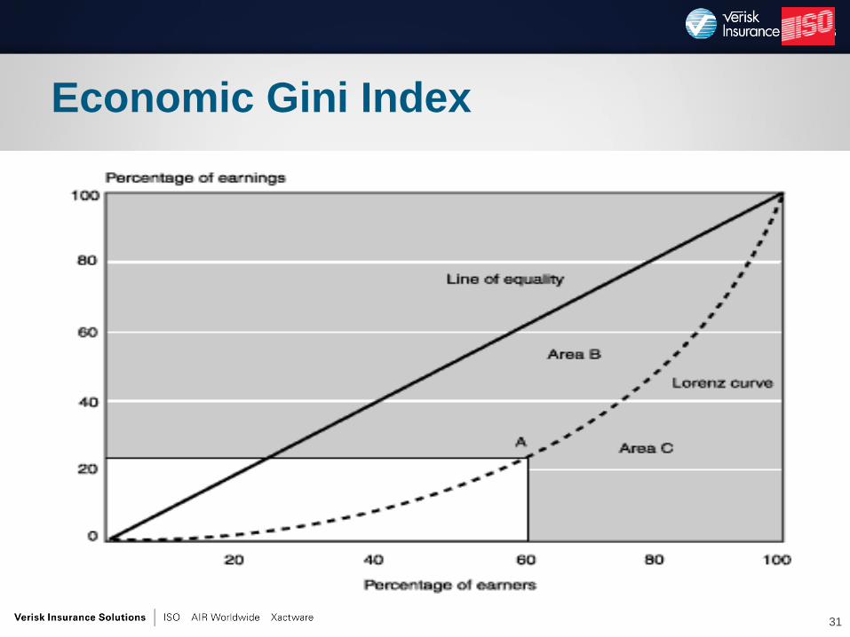
Economic Gini Index

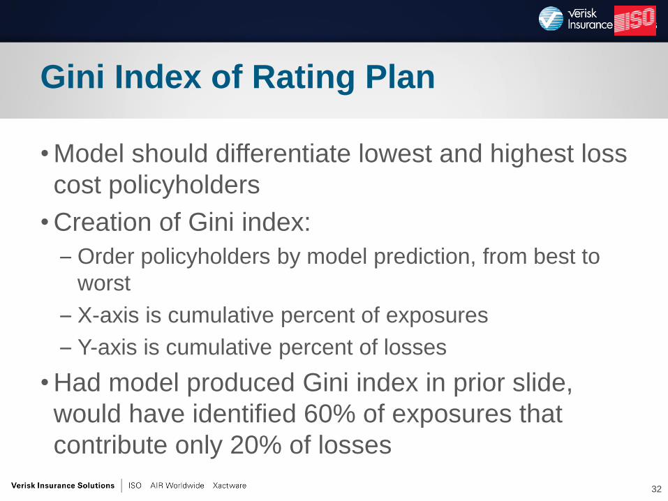
• Model should differentiate lowest and highest loss

cost policyholders

• Creation of Gini index:

– Order policyholders by model prediction, from best to

worst

– X-axis is cumulative percent of exposures

– Y-axis is cumulative percent of losses

• Had model produced Gini index in prior slide,

would have identified 60% of exposures that

contribute only 20% of losses

32

Gini Index of Rating Plan

•Cross-validation

–Split data into subsets (e.g. by time period)

–Refit model on each subset

–Compare model parameter estimates

•Bootstrapping

–Refit model on many bootstrapped samples

–Calculate variability of parameter estimates

•Deletion of influential records

33

Methods for Testing Model Stability

•Cook’s Distance: Statistical measure of the

impact each record has on the overall model

–Excellent tool for identifying errors or anomalies

–Deletion of records with high Cook’s Distance

may significantly change model results, and so

this procedure can be used to test stability

•DFBETA: Influence on a certain parameter

• Influence is not to be confused with leverage

34

Measures of Influence

For Further Reference

• Anderson, Duncan, et. al., A Practitioner’s Guide to Generalized Linear Models, CAS Discussion Paper Program, 2004

35

For Further Reference

• McCullagh, Peter and Nelder, John A., Generalized Linear Models, 2nd Ed., Chapman & Hall, 1989

36

For Further Reference

• De Jong, Piet and Heller, Gillian, Generalized Linear Models for Insurance Data, Cambridge University Press, 2008

37

For Further Reference

• Ohlsson, Esbjörn and Johansson, Björn, Non-Life Pricing with Generalized Linear Models, Springer, 2010

38

Introduction to Predictive Modeling Using GLMs

A Practitioner’s Viewpoint

Dan Tevet, FCAS, MAAA

Anand Khare, FCAS, MAAA, CPCU

39