Control Engineering Practice 11 (2003) 649–664

A practical multiple model adaptive strategy for multivariable modelpredictive control

Danielle Dougherty, Doug Cooper*

Chemical Engineering Department, 191 Auditorium Rd U-3222, University of Connecticut, Storrs, CT 06269-3222, USA

Received 16 July 2002; accepted 30 July 2002

Abstract

Model predictive control (MPC) has become the leading form of advanced multivariable control in the chemical process industry.

The objective of this work is to introduce a multiple model adaptive control strategy for multivariable dynamic matrix control

(DMC). The novelty of the strategy lies in several subtle but significant details. One contribution is that the method combines the

output of multiple linear DMC controllers, each with their own step response model describing process dynamics at a specific level

of operation. The final output forwarded to the controller is an interpolation of the individual controller outputs weighted based on

the current value of the measured process variable. Another contribution is that the approach does not introduce additional

computational complexity, but rather, relies on traditional DMC design methods. This makes it readily available to the industrial

practitioner.

r 2002 Published by Elsevier Science Ltd.

Keywords: Model predictive control; Dynamic matrix control; Adaptive control; Multiple models; Industrial control

1. Introduction

Model predictive control (MPC) has established itselfin industry as an important form of advanced control(Townsend & Irwin, 2001). Since the advent of MPC,various model predictive controllers have evolved toaddress an array of control issues (Garc!ıa, Prett, &Morari, 1989; Froisy, 1994). Dynamic matrix control(DMC) (Cutler & Ramaker, 1980) is the most popularMPC algorithm used in the chemical process industrytoday (Qin & Badgwell, 1996; Townsend, Lightbody,Brown, & Irwin, 1998). A major part of DMCs appeal inindustry stems from the use of a linear finite stepresponse model of the process and a quadraticperformance objective function. The objective functionis minimized over a prediction horizon to compute theoptimal controller output moves as a least squaresproblem.

When DMC is employed on nonlinear chemicalprocesses, the application of this linear model basedcontroller is limited to relatively small operating regions.

Specifically, if the computations are based entirely onthe model prediction (i.e. no constraints are active), theaccuracy of the model has significant effect on theperformance of the closed loop system (Gopinath,Bequette, Roy, Kaufman, & Yu, 1995). Hence, thecapabilities of DMC will degrade as the operating levelmoves away from the original design level of operation.

To maintain the performance of the controller over awide range of operating levels, a multiple modeladaptive control (MMAC) strategy for DMC has beendeveloped. While MMAC will not capture severenonlinear dynamic behavior, it will provide significantbenefits over linear controllers. The work focuses on aMMAC strategy for processes that are stationary intime, but nonlinear with respect to the operating level.This method is not applicable to processes where thegain of the process changes sign.

The method of approach is to construct a small set ofDMC process models that span the range of expectedoperation. By combining the process models to form anonlinear approximation of the plant, the true plantbehavior can be reasonably achieved (Banerjee, Arkun,Ogunnaike, & Pearson, 1997). If linear process modelsand controllers are employed, the wealth of design andtuning strategies for the linear controllers can be used.

*Corresponding author. Tel.: +860-486-4092; fax: +860-486-2959.

E-mail addresses: danielle.dougherty@uconn.edu (D. Dougherty),

cooper@engr.uconn.edu (D. Cooper).

0967-0661/02/$ - see front matter r 2002 Published by Elsevier Science Ltd.

PII: S 0 9 6 7 - 0 6 6 1 ( 0 2 ) 0 0 1 7 0 - 3

This is a benefit to the control practitioner since they donot have complete knowledge of the nonlinear controlstrategies currently available in the literature (Schott &Bequette, 1991; Townsend et al., 1998).

The accuracy of the nonlinear approximation can beincreased by combining more models. However, this isexpensive because each model requires the collection ofplant data at a different level of operation. The numberof DMC process models ultimately employed is apractical determination made by the control practitioneron a case-by-case basis. In most cases, the practitionerwill balance the expense of collecting data with the needto improve the nonlinear approximation.

The novelty of this work lies in the specific details ofthe strategy. The technique involves designing andcombining multiple linear DMC controllers. Each con-troller has their own step response model that describesthe process dynamics at a specific level of operation. Thefinal controller outputs forwarded to the controllers areobtained by interpolating between the individual con-troller outputs based on the values of the measuredprocess variables. The tuning parameters for eachcontroller are obtained by using already published tuningguidelines. The result is a simple and easy to use methodfor adapting the control performance without increasingthe computational complexity of the control algorithm.

2. Background

In the past, adding an adaptive mechanism to MPChas been approached in a number of ways. Researchershave primarily focused on updating the internal processmodel used in the control algorithm. Several articlesreview various adaptive control mechanisms for con-trolling nonlinear processes (Seborg, Edgar, & Shah,1986; Bequette, 1991; Di Marco, Semino, & Brambilla,1997). In addition, Qin and Badgwell (2000) provide agood overview of nonlinear MPC applications that arecurrently available in industry. As illustrated by theseworks, the adaptive control mechanisms consider theuse of a nonlinear analytical model, combinations oflinear empirical models or some mixture of both.

A popular approach for adaptive MPC is to linearize thenonlinear analytical model at each sampling instance(Garc!ıa, 1984; Krishnan & Kosanovich, 1998; Gattu &Zafiriou, 1992, 1995; Lee & Ricker, 1994; Gopinath et al.,1995; Peterson, Hern!andez, Arkun, & Schork, 1992).Others have used the nonlinear analytical model to obtainlinear state space models at different operating levels. Thesemodels are then weighted using a Bayesian estimator ateach sampling instance to obtain an adapted internalprocess model (Lakshmanan & Arkun, 1999; Bodizs,Szeifert, & Chovan, 1999). Analytical models are difficultto obtain due to the underlying physics and chemistry of theprocess, and they are often too complex to employ directlyin the optimization calculation (Morari & Lee, 1999).

Simple nonlinear output transformations have beenapplied to the nonlinear analytical equations in order tolinearize the process model (Georgiou, Georgakis,

Nomenclature

ars;i ith unit step response coefficient forcontroller output s on process variable r

A dynamic matrixd prediction error%e vector of predicted errorsi indexk discrete dead timeK process gainl level of operation indexM control horizon (number of controller out-

put moves)N model horizon (process settling time in

samples)P prediction horizonR number of measured process variablesS number of controller outputsT sample timeu controller output variablexl;s weighting factor#yr predicted process variable for process variable r

yr;l value of process variable r at level l

ymeas;r current measurement of process variable r

Greek symbols

Duadap;s adapted controller output move forcontroller output s

D%u vector of controller output moves to bedetermined

g2r controlled variable weight (equal concern

factor) in MIMO DMCKTK matrix of move suppression coefficientsl2

s move suppression coefficients (controlleroutput weight) in MIMO DMC

CTC matrix of controlled variable weightsy effective dead time of processt overall process time constanttp1

1st process time constanttp2 2nd process time constant

Abbreviations

DMC Dynamic matrix controlFOPDT First order plus dead timeMIMO Multiple-input multiple-outputMMAC Multiple model adaptive controlMPC Model predictive controlPID Proportional integral derivativePOR Peak overshoot ratio

D. Dougherty, D. Cooper / Control Engineering Practice 11 (2003) 649–664650

& Luyben, 1988). While this method improves theperformance of DMC for nonlinear processes, outputtransformations can be challenging to design for someapplications. The nonlinear analytical model can beused directly in the control algorithm by modifying theperformance objective functions or process constraints(Ganguly & Saraf, 1993; Sistu, Gopinath, & Bequette,1993; Katende, Jutan, & Corless, 1998; Xie, Zhou, Jin,& Xu, 2000), or used in combination with empiricalmodels to form a model reference adaptive controller(e.g., Gundala, Hoo, & Piovoso, 2000).

Recursive formulations update the parameters of theprocess model as new plant measurements becomeavailable at each sampling instance (McIntosh, Shah, &Fisher, 1991; Maiti, Kapoor, & Saraf, 1994, 1995; Ozkan& Camurdan, 1998; Liu & Daley, 1999; Yoon, Yang,Lee, & Kwon, 1999; Zou & Gupta, 1999; Chikkula &Lee, 2000). Recursive estimation schemes have well-known problems including: convergence problems if thedata does not contain sufficient and persistent excitation,inaccurate model parameters if unmeasured disturbancesor noise influence the measurements, and sensitivity toprocess dead times and high noise levels.

A more practical adaptive strategy uses a gain andtime constant schedule for updating the process model(McDonald & McAvoy, 1987; Chow, Kuznetsoc, &Clarke, 1998). An extension of this method is to usemultiple models to update the process model. Linearmodels that described the system at various operatingpoints are developed based on plant measurements. Pastresearchers (e.g., Banerjee et al., 1997) have illustratedthat linear models can be combined in order to obtain anapproximation of the process that approaches itstrue behavior. Two different multiple model con-troller design methods can be employed to maintain theperformance of the controller over all operating levels.

In one case, a controller is designed for each level ofoperation. In the past, this methodology has beenapplied to generalized predictive control and propor-tional-integral-derivative controllers. The controllermoves are then weighted based on the prediction errorcalculated for each controller. The resulting weights areobtained using recursive identification such that theprediction error is minimized (Yu, Roy, Kaufman, &Bequette, 1992; Schott & Bequette, 1994).

Although the concept used in this paper is similar tothose listed above, there are some important differences.One of the differences of this approach is that thestrategy is applied directly to the DMC algorithm. Themethod is to design and combine multiple linear DMCcontrollers, each with their own step response model.Another contribution is that the proposed methodologydoes not introduce additional computation complexity.

For the other case, a single controller is used.Although this concept is not used in the proposedstrategy, the method is related. Gendron et al. (1993)

developed a multiple model pole placement controller.The process models were weighted based on the currentprocess variable measurement, and then the weightedmodel is used in a single controller. Rao, Aufderheide,and Bequette (1999) and Townsend and Irwin (2001)designed a multiple model adaptive model predictivecontroller. The processes models were combined basedon the prediction error and then the weighted model wasagain sent to a single controller.

Townsend et al. (1998) developed a nonlinear DMCcontroller that replaces the linear process model with a localmodel network. This local model network contains locallinear ARX models and is trained using a hybrid learningtechnique. From this local model network, the DMCcontroller is supplied with a weighted step response model.

Narendra and Xiang (2000) design multiple control-lers using both fixed and adaptive process models. Basedon the prediction error for each of these process models,a procedure is designed that switches between thecontrollers corresponding to the process model withthe lowest prediction error. This allows the controller toincorporate both time-invariant dynamics along withtime-varying dynamics.

3. Multivariable DMC

Multivariable DMC has been discussed extensively bypast researchers (Cutler & Ramaker, 1980; Marchetti,Mellichamp, & Seborg, 1983) and is summarized herefor the convenience of the reader. For a system with S

controller outputs and R measured process variables,the multivariable DMC quadratic performance objec-tive function has the form (Garc!ıa & Morshedi, 1986)

Min JD%u

¼ ½%e � AD%u�TCTC½%e � AD%u� þ ½D%u�TKTK½D%u�; ð1Þ

subject to

#yr;minp #yrp #yr;max;

D%us;minpD%uspD%us;max;

%us;minp%usp%us;max: ð2Þ

A closed form solution to the multivariable DMCperformance objective (Eq. (1)) results in the uncon-strained multivariable DMC control law (Garc!ıa &Morshedi, 1986):

D%u ¼ ðATCTCA þ KTKÞ�1ATCTC%e: ð3Þ

Here, A is the multivariable dynamic matrix formedfrom unit step response coefficients of each controlleroutput to measured process variable pair; %e is the vectorof predicted errors for the R measured process variablesover the next P sampling instants (prediction horizon);D%u is the vector of controller output changes for the S

controller output computed for the next M samplinginstants (control horizon); #yr is the predicted process

D. Dougherty, D. Cooper / Control Engineering Practice 11 (2003) 649–664 651

variable profile for the rth measured process variableover the next P sampling instances; CTC is the matrix ofcontrolled variable weights and KTK is the matrix ofmove suppression coefficients.

KTK is a square diagonal matrix of dimensions(MS � MS). The leading diagonal elements of the ith(M � M) matrix block along the diagonal of KTK arel2

i : All off-diagonal elements are zero. Hence, in themultivariable DMC control law (Eq. (3)), the movesuppression coefficients that are added to the leadingdiagonal of the system matrix, ðATCTCAÞ; are l2

i

(i ¼ 1; 2;y;S). Similarly, the (PR � PR) matrix ofcontrolled variable weights, CTC; has the leadingdiagonal elements as g2

i (i ¼ 1; 2;y;R). Again, all off-diagonal elements are zero.

The implementation of DMC involves using stepresponse coefficients to predict the future processvariable behavior, #yrðk þ 1Þ; over the prediction hor-izon. This profile is corrected by adding to it estimates ofthe disturbance. The disturbance estimates are calcu-lated as the difference between the current measurementof the process variable and the current value of thepredicted process variable at the present sample time.The disturbance estimate is assumed constant over theprediction horizon. Then, Eq. (1) or (3) is solved on-lineto determine the optimal values of the controller outputmoves. Only the first element of the vector is imple-mented and the entire procedure is repeated at the nextsampling instance.

4. Formulation of an MMAC strategy for DMC

The method of approach in this work focuses onweighting a minimum of three linear DMC controllersbased on the current measurement of the processvariable. Three linear controllers are used here becauseas mentioned previously, collecting plant data is difficultand time consuming. The method can easily beexpanded to more models if desired by the practitioner.

4.1. Non-adaptive DMC Implementation

For comparison, a non-adaptive DMC controller isdesigned and present along side the adaptive methodusing the tuning rules given by Shridhar and Cooper(1997, 1998). Table 1 displays the guidelines fordetermining the tuning parameters for non-adaptiveDMC. The tuning parameters and the step responsecoefficients are calculated offline prior to the start-up ofthe non-adaptive DMC controller and remain constantduring operation.

As presented in Table 1, step 1 of these rules is basedon fitting the controller output to measured processvariable dynamics for each sub-process relating the sthcontroller output to the rth process variable at thedesign level of operation with a first-order plus deadtime (FOPDT) model approximation. Although anFOPDT model approximation does not capture all thefeatures of higher order processes, it often reasonably

Table 1

Non-adaptive DMC tuning strategy

1. Approximate the process dynamics of all controller output to measured process variable pairs with FOPDT models:

yrðsÞusðsÞ

¼Krse

�yrss

trss þ 1ðr ¼ 1; 2;y;R; s ¼ 1; 2;y;SÞ

2. Select the sample time as close as possible to:

Trs ¼ Maxð0:1trs; 0:5yrsÞ;

ðr ¼ 1; 2;y;R; s ¼ 1; 2;y;SÞ

T ¼ MinðTrsÞ;

3. Compute the prediction horizon, P; and the model horizon, N:

P ¼ N ¼ Max5trs

Tþ krs

� �where krs ¼

yrs

Tþ 1

� �ðr ¼ 1; 2;y;R; s ¼ 1; 2;y;SÞ

4. Compute a control horizon, M:

M ¼ Maxtrs

Tþ krs

� �ðr ¼ 1; 2;y;R; s ¼ 1; 2;y;SÞ

5. Select the controlled variable weights, g2r ; to scale process variable units to be the same.

6. Compute the move suppression coefficients, l2s :

l2s ¼

M

10

XR

r¼1

g2r K2

rs P � krs �3

2

trs

Tþ 2 �

ðM � 1Þ2

� �� ðs ¼ 1; 2;y;SÞ

7. Implement DMC using the traditional step response matrix of the actual process and the initial values of the parameters computed in steps 1–6.

D. Dougherty, D. Cooper / Control Engineering Practice 11 (2003) 649–664652

describes the process gain, overall time constant andeffective dead time of such processes (Cohen & Coon,1953; Stauffer, 2001).

An FOPDT model fit provides four critical pieces ofinformation useful for controller design. Specifically, K

indicates the size and direction of the process variableresponse to a control move, t describes the speed of theresponse, and y tells the delay prior to when theresponse begins. Previous research for tuning DMC(Shridhar & Cooper, 1997, 1998) has demonstrated thatthis information is often sufficient to achieve desirableclosed loop DMC performance at the specified designlevel of operation. As long as the FOPDT modelparameters are identified such that they describe thesystem reasonably, the tuning strategy should besuccessful even for higher order processes (Shridhar &Cooper, 1997, 1998).

Step 2 involves the selection of a sample time, T : TheFOPDT parameters, from step 1, provide a convenientmethod for obtaining T : The value of T given in Table 1balances the desire for a low computation load (a largeT) with the need to properly track the evolving dynamicbehavior (a small T). Ljung (1987) confirms thesefindings, stating that too slow of a sampling rate willlead to information losses, and too fast of a samplingrate could lead to numerically sensitive procedures.Many control computers restrict the choice of T (e.g.,Franklin & Powell, 1980; (Astr .om & Wittenmark, 1984).Recognizing this, the remaining tuning rules permitvalues of T other than the recommended value given inTable 1.

Step 3 computes the prediction horizon, P; and themodel horizon, N ; in samples as the settling time of theslowest sub-process in the multivariable system. Notethat both N and P cannot be selected independent of thesample time.

A larger P improves the nominal stability of theclosed loop. For this reason P is calculated such thatit includes the steady-state effect of all past contro-ller output moves, i.e. it is calculated as the openloop settling time of the slowest FOPDT modelapproximation.

In addition, it is important that N be equal to theopen loop settling time of the slowest sub-process toavoid truncation error in the predicted process variableprofiles. Table 1 computes N as the settling time of theslowest FOPDT model approximation. This value islong enough to avoid the instabilities that can otherwiseresult since truncation of the model horizon misrepre-sents the effect of controller output moves in thepredicted process variable profile (Lundstr .om, Lee,Morari, & Skogestad, 1995).

Step 4 computes the control horizon, M; equal to63.2% of the settling time of the slowest sub-process inthe multivariable system. This ensures M to be longenough such that the results of the control actions are

clearly evidenced in the response of the measuredprocess variable.

Step 5 requires the selection of the controlledvariable weights, g2

r : In most cases, the controlledvariable weights are set equal to one. However,the practitioner is free to select these values torecast the measured process variables into thesame units. Or, the practitioner can use these parametersto achieve tighter control of a particular measuredprocess variable by selectively increasing its relativeweight.

Step 6 computes the move suppression coefficients, l2s :

Its primary role in DMC is to suppress aggressivecontroller actions. When the control horizon is 1(M ¼ 1), no move suppression coefficient is needed(l ¼ 0). If the control horizon is greater than 1 (M > 1),then the analytical equation given in Table 1 is used.

Step 7 summarizes the tuning parameters for multi-variable DMC. Once the tuning parameters have beendetermined, the unit step response coefficients, ars;i

(i ¼ 1; 2;y;N; r ¼ 1; 2;y;R; s ¼ 1; 2;y;S), for con-troller output s on measured process variable r arecalculated.

Step response coefficients for the internal DMCprocess model do not use an FOPDT approximation.Rather, actual process data is employed as is typical forDMC. The process data is generated by introducing apositive step in one controller output with the process atsteady state and all the controllers in manual mode. Inaddition, all other controller output variables mustremain constant. From the instant the step change ismade, the response of each process variable is recordedas it evolves and settles at a new steady state. For a stepin the controller output of arbitrary size, the responsedata is normalized by dividing through by the size of thecontroller output step to yield the unit step response.This is performed for each controller output tomeasured process variable pair, and it is necessary tomake the controller output step large enough such thatnoise in the process variable measurement does notmask the true process behavior.

For simplicity, the remainder of the algorithm isformulated here for a system with two controlleroutputs and two process variables. The method can bedirectly extended to more complex processes.

For a two-by-two system, the multivariable dynamicmatrix, A; is formulated using the first P step responsecoefficients:

A ¼A11 A12

A21 A22

" #2P�2M

; ð4Þ

where A11 is constructed from the step response ofprocess variable 1 (PV1) obtained by a step change in

D. Dougherty, D. Cooper / Control Engineering Practice 11 (2003) 649–664 653

controller output 1 (CO1). Aij is given by

Aij ¼

aij;1 0 0 ? 0

aij;2 aij;1 0 0

aij;3 aij;2 aij;1 & 0

^ ^ ^ 0

aij;M aij;M�1 aij;M�2 aij;1

^ ^ ^ ^

aij;P aij;P�1 aij;P�2 ? aij;P�Mþ1

2666666666664

3777777777775

P�M

:

ð5Þ

Using Eqs. (1) and (2) for constrained DMC orEq. (3) for unconstrained systems, a vector of (SM)controller output moves is computed over the controlhorizon:

D%u ¼

Du1ðnÞ

Du1ðn þ 1Þ

Du1ðn þ 2Þ

^

Du1ðn þ M � 1Þ

Du2ðnÞ

Du2ðn þ 1Þ

Du2ðn þ 2Þ

^

Du2ðn þ M � 1Þ

266666666666666666664

377777777777777777775

2M�1

; ð6Þ

where Du1ðnÞ is the move implemented for CO1 andDu2ðnÞ is the move implemented for controller output 2(CO2).

4.2. The adaptive strategy

The adaptive DMC strategy builds on the non-adaptive formal tuning rule and the DMC control movecalculation. As displayed in Fig. 1, the approach for theadaptive strategy involves designing three non-adaptiveDMC controllers. Each controller has a model-basedoptimizer and a model-based predictor. The approachdescribed here involves designing and combining threenon-adaptive DMC controllers. However, this techni-que can involve designing and combining any number ofnon-adaptive controllers.

As explained below, all use the same values for T ; P;N; M ; and g2

r ; while l2s varies for each controller. The

three controllers each compute their own control action.These are then weighted and combined based on thevalue of the current measurements of each processvariable to yield a single set of control moves forwardedto the final control elements.

Although three controllers are employed here, themethod can be expanded to include as many local linearcontrollers as the practitioner would like. The use ofthree linear DMC controllers is the minimum needed to

reasonably control a nonlinear process. The more linearcontrollers that are used, the better the adaptivecontroller will perform. There are no theoretical guide-lines to illustrate how many linear controllers should beused in the adaptive control strategy to give optimalperformance (Yu et al., 1992). While this method willoften not capture the severe nonlinear behaviorsassociated with many processes, it will provide signifi-cant benefit over the non-adaptive DMC controller.

Implementation begins by collecting sets of step testdata at three levels of operation, one at a lower, middleand upper level of the expected operating range for eachsub-process relating the sth controller output to the rthmeasured process variable. For example, if there are twocontroller outputs and two measured process variables,then 12 sets of step test data will be needed for theadaptive DMC strategy. Each of the process modelsshould describe the process dynamics around the pointin which the data was collected. Two of the operatingpoints should be at the upper and lower extremes ofthe expected operating region to ensure that thenonlinear approximation reasonably describes the ac-tual process over the entire operating range (Di Marcoet al., 1997). The third operating point should be aroundthe middle of the expected operating region. Theoperating levels are defined as a specific value for eachof r measured process variables, yrl ; where l ¼ 1; 2, 3 arefor the lower, middle and upper level of operation,respectively.

Each data set is fit with a linear FOPDT model for usein the tuning correlations. The data itself is used toformulate the step response coefficients. The tuningparameters for the adaptive DMC strategy are com-puted by employing the formal tuning rules given inTable 1.

Here, T is selected as close as possible to the smallestTrsl from the data sets, or:

Trsl ¼ Maxð0:1trsl ; 0:5yrslÞ;

T ¼ MinðTrslÞ;

ðr ¼ 1; 2;y;R; s ¼ 1; 2;y;S; l ¼ 1; 2; 3Þ: ð7Þ

This ensures that when the process is operating in thelevel with the fastest dynamics, the sample time is fastenough to capture the process behavior. Since manycontrol computers restrict the choice of T (e.g., Franklin& Powell, 1980; (Astr .om & Wittenmark, 1984), theremaining tuning rules permit values of T other thanthat computed by Eq. (7) to be used.

The tuning parameters P; N ; and M are selected asthe maximum values:

P ¼ N ¼ Max5trsl

Tþ krsl

� �

ðr ¼ 1; 2;y;R; s ¼ 1; 2;y;S; l ¼ 1; 2; 3Þ; ð8aÞ

D. Dougherty, D. Cooper / Control Engineering Practice 11 (2003) 649–664654

where

krsl ¼yrsl

Tþ 1

� �; ð8bÞ

M ¼ Maxtrsl

Tþ krsl

� �ðr ¼ 1; 2; 3;y;R; s ¼ 1; 2;y;S; l ¼ 1; 2; 3Þ: ð8cÞ

Thus, the horizons will always be long enough to capturethe slowest dynamic behaviors in the range of operation.Truncation of any of the horizons (prediction, model orcontrol) can result in instabilities in the closed system.

The controlled variable weights are usually set equalto one. However, the practitioner is free to select thesevalues to recast the measured process variables into thesame units. For example, the span of each processvariable can be used to convert the units for the processvariable to percentage. Or, the practitioner can use theseparameters to achieve tighter control of a particularmeasured process variable by selectively increasing itsrelative weight.

Even though the above tuning parameters remainfixed upon implementation, success in this adaptivestrategy requires that l2

s vary based upon each data set.Since each data set will have different values for Krs; trs;

and yrs; the value of l2sl calculated for each data set must

reflect this difference, or

l2sl ¼

M

10

XR

r¼1

g2rlK

2rsl P � krsl �

3

2

trsl

Tþ 2 �

ðM � 1Þ2

� ��

ðs ¼ 1; 2;y;S; l ¼ 1; 2; 3Þ: ð9Þ

Note that the calculation of l2sl is based upon the overall

M and not on the control horizon calculated for eachtest set of data for each sub-process in the multivariablesystem. This allows l2

sl to suppress aggressive controlactions over the entire control horizon. Similar to non-adaptive DMC, Eq. (8) is valid for a control horizongreater than 1 (M > 1), and if the control horizon is 1(M ¼ 1), then no move suppression coefficient is used(l2

sl ¼ 0).Upon implementation, the MMAC strategy for DMC

calculates three non-adaptive DMC controller outputmoves, one for each level of operation. The adaptivecontroller output moves, Duadap;s; are a weighted averageof each linear controller output move:

Duadap;s ¼X3

l¼1

xl;sDuð1Þl;s

ðs ¼ 1; 2;y;S; l ¼ 1; 2; 3Þ; ð10Þ

Process

Processvariable

First move in controller output

profile

y (n)

Model BasedOptimizer

Desiredset pointtrajectory

ysp(n + j )

ysp(n + j )

Model BasedPredictor

DMC 1

Predicted processvariable profile

-+

Desiredset pointtrajectoryysp(n + j )

Desiredset pointtrajectoryysp(n + j )

DMC 2

ControllerWeightingCalculation

DMC 3

∆uadap,s(n)

++

Fig. 1. Schematic of multiple model adaptive DMC strategy.

D. Dougherty, D. Cooper / Control Engineering Practice 11 (2003) 649–664 655

where xl;s is a weighting factor. If ymeas;r is the actualvalue of the measured process variable r at the currentsample time, then

If ymeas;rXy3;r then

x1;s ¼ 0; x2;s ¼ 0; x3;s ¼ 1: ð11Þ

If y2;roymeas;roy3;r then

x1;s ¼ 0; x2;s ¼ 1 � x3;s; x3;s ¼ymeas;r � y2;r

y3;r � y2;r: ð12Þ

If y1;roymeas;roy2;r then

x1;s ¼ 1 � x2;s; x2;s ¼ymeas;r � y1;r

y2;r � y1;r; x3;s ¼ 0: ð13Þ

If ymeas;rpy1;r then

x1;s ¼ 1; x2;s ¼ 0; x3;s ¼ 0: ð14Þ

In the event that ymeas;r ¼ y2;r; then the adaptivecontroller output move equals the value associated withthe middle data set. Hence, the weighting factors are inthe range of [0,1]. The values of the adaptive controlleroutputs finally implemented are calculated as

uðnÞs ¼ uðn � 1Þs þ Duadap;s ðs ¼ 1; 2;y;SÞ: ð15Þ

Theoretical studies are needed to address the issue ofclosed loop stability over the entire range of nonlinearoperation. It has been shown by past researchers(Greene & Willsky, 1980) that the overall MMACsystem may not be stable even if each individualcontroller is stable over the entire range of operation.In addition, Narendra and Xiang (2000) address theissue of stability for linear time-invariant discretesystems using MMAC. The results included a proof ofglobal stability for the overall system.

5. Demonstration of multivariable adaptive DMC

The adaptive DMC algorithm is demonstrated herefor three process simulations, a synthetic transferfunction model, a multi-tank process, and rigorousdistillation column.

5.1. Transfer function model

The transfer function model has two measuredprocess variables and two controller outputs. A changein either controller output affects both process variables.Each controller output to measured process variablepair is a sub-process. In this example there are foursub-processes, which include controller output 1 (CO1)to process variable 1 (PV1), controller output 1 (CO1) toprocess variable 2 (PV2), controller output 2 (CO2) toprocess variable 1 (PV1), and controller output 2 (CO2)to process variable 2 (PV2).

To form nonlinear models, three different transferfunctions are combined using a linear weighting

function. The general form of each transfer function is

GpðsÞ ¼Ke�yS

ðtP1s þ 1ÞðtP2

s þ 1Þ: ð16Þ

Each of the three transfer functions has differentparameter values, and each exactly describes thebehavior of the process at a specific value of themeasured process variable. At intermediate values ofthe measured process variable, the transfer functioncontributions are combined to yield a continuallychanging dynamic behavior. This methodology is usedto construct nonlinear models for the four sub-processes.

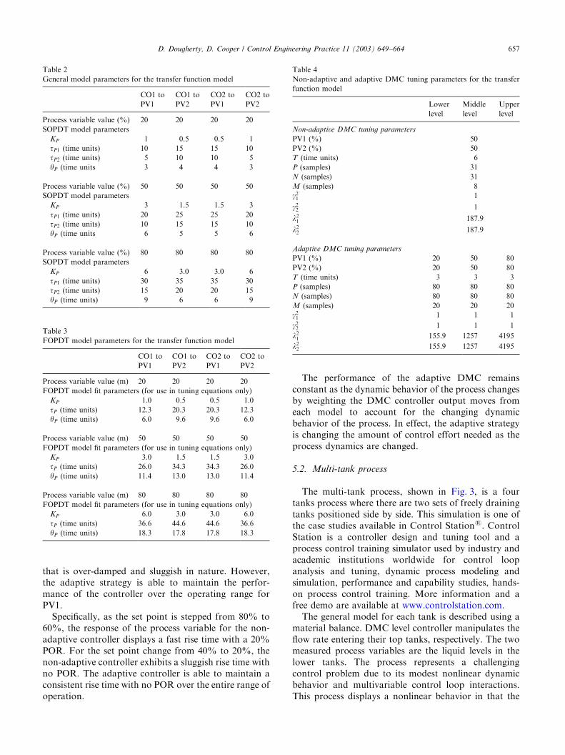
Table 2 lists the parameters used for each of the threetransfer functions. As listed, a model is defined atmeasured process variables value of 20%, 50%, and80%. To make the application nonlinear, the processgains change by 600% over the range of operation. Also,dead time and time constants change by as much as200%.

Dynamic tests are performed by pulsing each con-troller output at each level of operation, yielding six setsof test data. Three data sets were collected at PV1 levelsof 20%, 50%, and 80%, and three data sets werecollected at PV2 levels of 20%, 50% and 80%.Following the adaptive DMC design procedure de-scribed previously, an FOPDT model is fit to each dataset to yield the parameters listed in Table 3. The FOPDTparameters are then used in the equations in Table 1 toobtain the non-adaptive DMC tuning parameters listedin Table 4.

Table 4 also lists the tuning parameters for theadaptive DMC strategy obtained by using Eqs. (7)–(9).Note that as described in the adaptive strategy, all threecontrollers use the same value for T ; P; N; M ; and g2

r ;while l2

s varies for each controller. This ensures that thesample time is short enough to capture the fastestdynamic behaviors while the horizons are long enoughto capture the slowest dynamic behaviors in the range ofoperation.

The control objective in this study is set point trackingof PV1 across the range of nonlinear operation. Thedesign goal is a fast rise time with no peak overshootratio (POR). Non-adaptive DMC uses the tuningparameters associated with the middle level of operation(i.e. the measured process variable equals 50%). It isreasonable to design the non-adaptive controller basedon the middle level of operation because this will yield acompromise in performance over the range of dynamicbehaviors.

Fig. 2 shows the response of PV1 for both the non-adaptive and adaptive DMC implementations. Asillustrated by the figure, the performance of the non-adaptive DMC varies as the dynamic behavior of theprocess changes. As the set point is stepped from 80%down to 20%, the performance of the non-adaptivecontroller varies from an under-damped response to one

D. Dougherty, D. Cooper / Control Engineering Practice 11 (2003) 649–664656

that is over-damped and sluggish in nature. However,the adaptive strategy is able to maintain the perfor-mance of the controller over the operating range forPV1.

Specifically, as the set point is stepped from 80% to60%, the response of the process variable for the non-adaptive controller displays a fast rise time with a 20%POR. For the set point change from 40% to 20%, thenon-adaptive controller exhibits a sluggish rise time withno POR. The adaptive controller is able to maintain aconsistent rise time with no POR over the entire range ofoperation.

The performance of the adaptive DMC remainsconstant as the dynamic behavior of the process changesby weighting the DMC controller output moves fromeach model to account for the changing dynamicbehavior of the process. In effect, the adaptive strategyis changing the amount of control effort needed as theprocess dynamics are changed.

5.2. Multi-tank process

The multi-tank process, shown in Fig. 3, is a fourtanks process where there are two sets of freely drainingtanks positioned side by side. This simulation is one ofthe case studies available in Control Stations. ControlStation is a controller design and tuning tool and aprocess control training simulator used by industry andacademic institutions worldwide for control loopanalysis and tuning, dynamic process modeling andsimulation, performance and capability studies, hands-on process control training. More information and afree demo are available at www.controlstation.com.

The general model for each tank is described using amaterial balance. DMC level controller manipulates theflow rate entering their top tanks, respectively. The twomeasured process variables are the liquid levels in thelower tanks. The process represents a challengingcontrol problem due to its modest nonlinear dynamicbehavior and multivariable control loop interactions.This process displays a nonlinear behavior in that the

Table 2

General model parameters for the transfer function model

CO1 to

PV1

CO1 to

PV2

CO2 to

PV1

CO2 to

PV2

Process variable value (%) 20 20 20 20

SOPDT model parameters

KP 1 0.5 0.5 1

tP1 (time units) 10 15 15 10

tP2 (time units) 5 10 10 5

yP (time units 3 4 4 3

Process variable value (%) 50 50 50 50

SOPDT model parameters

KP 3 1.5 1.5 3

tP1 (time units) 20 25 25 20

tP2 (time units) 10 15 15 10

yP (time units 6 5 5 6

Process variable value (%) 80 80 80 80

SOPDT model parameters

KP 6 3.0 3.0 6

tP1 (time units) 30 35 35 30

tP2 (time units) 15 20 20 15

yP (time units) 9 6 6 9

Table 3

FOPDT model parameters for the transfer function model

CO1 to

PV1

CO1 to

PV2

CO2 to

PV1

CO2 to

PV2

Process variable value (m) 20 20 20 20

FOPDT model fit parameters (for use in tuning equations only)

KP 1.0 0.5 0.5 1.0

tP (time units) 12.3 20.3 20.3 12.3

yP (time units) 6.0 9.6 9.6 6.0

Process variable value (m) 50 50 50 50

FOPDT model fit parameters (for use in tuning equations only)

KP 3.0 1.5 1.5 3.0

tP (time units) 26.0 34.3 34.3 26.0

yP (time units) 11.4 13.0 13.0 11.4

Process variable value (m) 80 80 80 80

FOPDT model fit parameters (for use in tuning equations only)

KP 6.0 3.0 3.0 6.0

tP (time units) 36.6 44.6 44.6 36.6

yP (time units) 18.3 17.8 17.8 18.3

Table 4

Non-adaptive and adaptive DMC tuning parameters for the transfer

function model

Lower

level

Middle

level

Upper

level

Non-adaptive DMC tuning parameters

PV1 (%) 50

PV2 (%) 50

T (time units) 6

P (samples) 31

N (samples) 31

M (samples) 8

g21 1

g22 1

l21 187.9

l22 187.9

Adaptive DMC tuning parameters

PV1 (%) 20 50 80

PV2 (%) 20 50 80

T (time units) 3 3 3

P (samples) 80 80 80

N (samples) 80 80 80

M (samples) 20 20 20

g21 1 1 1

g22 1 1 1

l21 155.9 1257 4195

l22 155.9 1257 4195

D. Dougherty, D. Cooper / Control Engineering Practice 11 (2003) 649–664 657

process gains for each sub-process change by at least afactor of 2 over the range of operation studied in thisexample.

Dynamic tests are performed by pulsing the controlleroutput at each level of operation, generating six sets of

test data. Three data sets were obtained at levels in tank1 of (measured PV1) of 1.5, 3.5 and 6.6 m. The otherthree data sets were obtained at levels in tank 2 of(measured PV2) of 1.4, 3.3 and 6.3 m. Following theprocedure just described in the previous example, each

10

20

30

40

50

60

70

80

90

0 200 400 600 800 1000 1200 1400 1600 1800 2000

Time

Proc

ess

Var

iabl

e 1

/ Set

Poi

nt 1

Adaptive DMC

Non-adaptive DMC

Set Point

Fig. 2. Response of PV1 for the transfer function model using non-adaptive and adaptive DMC.

manipulated variable 2

measuredprocess variable 2

manipulated variable 1

controlleroutput 1

controlleroutput 2

upper tank 1

lower tank 1

lower tank 2

LS

LS

upper tank 2

DMC

Fig. 3. Multi-tanks graphic.

D. Dougherty, D. Cooper / Control Engineering Practice 11 (2003) 649–664658

data set is fit with an FOPDT model (results listed inTable 5) and these parameters are used to compute thenon-adaptive and adaptive DMC tuning values (resultslisted in Table 6).

The control objective in this study is set point trackingacross the range of nonlinear operation. The designgoal in this study is a fast rise time with no POR.

Non-adaptive DMC uses the tuning parameters asso-ciated with the middle level of operation (i.e. PV1=3.5and PV2=3.3).

Fig. 4 shows the response of PV1 for both the non-adaptive and adaptive DMC implementations. As theset point is stepped from 5.5 to 1.5 m the behavior ofPV1 for non-adaptive DMC ranges from a response thatis under-damped to a response that is over-damped. Asthe process reaches higher tank levels, the processvariables response becomes more oscillatory.

As the set point is stepped from 5.5 to 4.5 m, theresponse of the non-adaptive controller displays a 5%POR. For the set point step from 2.5 to 1.5 m, the non-adaptive controller exhibits a sluggish rise time with noPOR. The adaptive controller exhibits no problems inmaintaining the design goal of a fast rise time with noPOR over the range of operation.

The disturbance rejection capabilities of the adaptiveand non-adaptive DMC controller were also studied.The disturbance is a secondary flow out of the lowertanks from a positive displacement pump, and isindependent of the liquid level except when the tanksare empty. The disturbance flow rate was stepped from 1to 2m3/min and then back to 1m3/min.

Fig. 5 shows the response of PV1 for both the non-adaptive and adaptive DMC implementations at a setpoint level of approximately 3.5 m. At this level ofoperation both the adaptive and non-adaptive QDMCcontrollers give similar performance. This is because thenon-adaptive controller was designed for a level of3.5 m. This is verified in Fig. 5.

Fig. 6 displays the response of PV1 for both the non-adaptive and adaptive DMC implementations at a setpoint level of approximately 1.5 m. At this level ofoperation the adaptive DMC controller should exhibitbetter disturbance rejection capabilities. This is becausethe tuning and model parameters for the non-adaptivecontroller are no longer valid. As displayed in Fig. 6, theadaptive controller outperforms the non-adaptive con-troller. The adaptive controller is able to reject thedisturbance quicker and return the height of the tankback to its set point faster.

As shown by these figures, the adaptive DMCcontroller is able to maintain better performance overall operating ranges. The adaptive strategy weights themultiple controller output moves in order to achieve thedesired performance at each level of operation.

5.3. Distillation column process

The distillation column simulation, shown in Fig. 7, isa tray-by-tray simulation model that is highly nonlinearand has strong interactive characteristics. This is one ofthe many multivariable simulations available in ControlStation. It is based on the system given by McCune andGallier (1973). For each tray, the reboiler and the

Table 5

FOPDT model parameters for the multi-tanks simulation

CO1 to

level 1

CO1 to

level 2

CO2 to

level 1

CO2 to

level 2

Process variable value (m) 1.5 1.4 1.5 1.4

FOPDT model fit parameters

KP 0.05 0.02 0.03 0.05

tP (min) 12.2 12.7 12.5 12.9

yP (min) 5.4 5.9 5.2 5.8

Process variable value (m) 3.5 3.3 3.5 3.3

FOPDT model fit parameters

KP 0.07 0.04 0.04 0.07

tP (min) 14.9 15.9 13.9 15.4

yP (min) 6.9 7.6 6.8 7

Process variable value (m) 6.6 6.3 6.6 6.3

FOPDT model fit parameters

KP 0.10 0.05 0.06 0.10

tP (min) 17.0 18.4 17.0 18.3

yP (min) 8.9 9.8 8.6 9.5

Table 6

Non-adaptive and adaptive DMC tuning parameters for the multi-

tanks simulation

Lower

level

Middle

level

Upper

level

Non-adaptive DMC tuning parameters

Level 1 (m) 3.5

Level 2 (m) 3.3

T (s) 180

P (samples) 29

N (samples) 29

M (samples) 8

g21 1

g22 1

l21 0.088

l22 0.088

Adaptive DMC tuning parameters

Level 1 (m) 1.5 3.5 6.6

Level 2 (m) 1.4 3.3 6.3

T (s) 180 180 180

P (samples) 34 34 34

N (samples) 34 34 34

M (samples) 10 10 10

g21 1 1 1

g22 1 1 1

l21 0.068 0.14 0.25

l22 0.079 0.14 0.26

D. Dougherty, D. Cooper / Control Engineering Practice 11 (2003) 649–664 659

condenser, differential equations are used to describe theoverall and component mass balances and algebraicequations are used for the energy balances. The stage

efficiencies are represented by the Murphy tray effi-ciency, and a linear hydraulic relationship is used todescribe the liquid flow from each tray as a function of

1

1.5

2

2.5

3

3.5

4

4.5

5

5.5

6

0 200 400 600 800 1000Time

Lev

el 1

/ Se

t Poi

nt 1

Non-Adaptive DMC

Adaptive DMC

Set Point

Fig. 4. Response of PV1 (level 1) for the multi-tanks process using non-adaptive and adaptive DMC.

3

3.1

3.2

3.3

3.4

3.5

3.6

3.7

3.8

3.9

4

0 100 200 300 400 500

Time (min)

Proc

ess

Var

iabl

e 1

/ Set

Poi

nt 1

Non-adaptive DMC

Adaptive DMC

Set Point

Fig. 5. Response of PV1 for the multi-tanks process using non-adaptive and adaptive DMC for disturbance rejection capabilities at a set point of

approximately 3.5m.

D. Dougherty, D. Cooper / Control Engineering Practice 11 (2003) 649–664660

the mass holdup. The simulation model separatesbenzene and toluene at constant pressure.

The column has two measured process variables andtwo manipulated variables. The reflux rate is used tocontrol the composition of benzene in the distillatestream and steam rate is used to control the composition

of benzene in the bottoms stream. The feed flow rateacts as a disturbance to the column.

Dynamic tests are performed by pulsing the controlleroutput at each level of operation, generating six sets oftest data. Three data sets were obtained at distillatecompositions (measured PV1) of 89.3%, 94.4% and

1.1

1.2

1.3

1.4

1.5

1.6

1.7

1.8

1.9

0 100 200 300 400 500

Time (min)

Proc

ess

Var

iabl

e 1

/ Set

Poi

nt 1

Non-adaptive DMC

Adaptive DMC

Set Point

Fig. 6. Response of PV1 for the multi-tanks process using non-adaptive and adaptive DMC for disturbance rejection capabilities at a set point of

approximately 1.5m.

disturbance variable

manipulated variable

measuredprocess variable

composition sensor

manipulated variable

composition sensor

.

measuredprocess variable

.

DM C

CS

CS

CS

CS

DMC

Fig. 7. Distillation column graphic.

D. Dougherty, D. Cooper / Control Engineering Practice 11 (2003) 649–664 661

98.7%. The other three data sets were obtained atbottom compositions (measured PV2) of 1.5%, 2.6%and 12.9%. Following the procedure just described inthe previous example, each data set is fit with an

FOPDT model (results listed in Table 7) and theseparameters are used to compute the non-adaptive andadaptive DMC tuning values (results listed in Table 8).

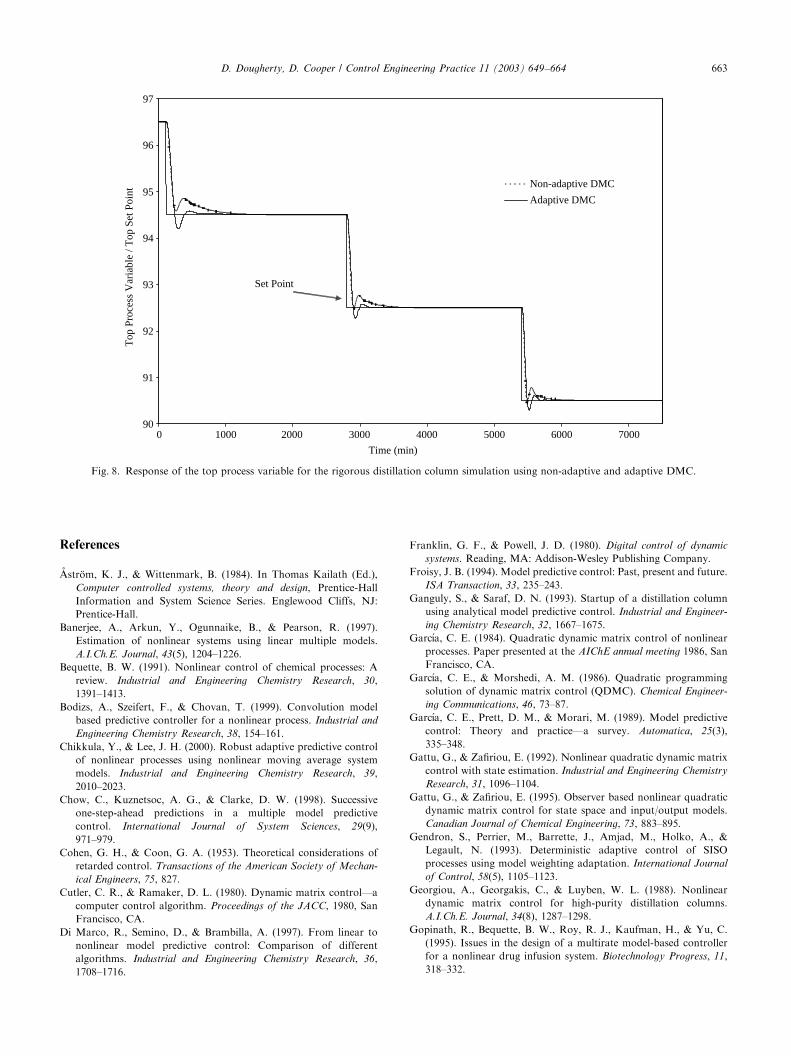
The control objective in this study is set point trackingacross the range of nonlinear operation. The designgoal in this study is a fast rise time and a quick settlingtime with no more than a 15% POR. Non-adaptiveDMC uses the tuning parameters associated with themiddle level of operation (i.e. PV1=94.4% andPV2=2.6%).

Fig. 8 displays the response of the top compositionfor both the non-adaptive and adaptive DMC imple-mentations. As the set point is stepped from 96.5% to94.5%, the response of the non-adaptive controllerdisplays no POR and a very long settling time comparedto the performance of the adaptive DMC controller.For the set point step from 94.5% to 92.5%, the non-adaptive controller exhibits no POR and a long settlingtime compared to the performance of the adaptiveDMC controller. For the set point step from 92.5%to 90.5%, the non-adaptive controller displays aslightly longer settling time than the adaptive controller.The adaptive controller exhibits no problems inmaintaining the design goal of a fast rise time andsettling time with a 15% POR over the range ofoperation.

The performance of the adaptive DMC implementa-tion is able to maintain the performance for PV1 over alloperating ranges. The adaptive strategy continues toweight the multiple controller output moves in order toachieve the desired performance.

6. Conclusions

A multiple model adaptive strategy for DMC hasbeen developed and the application and benefits of thisadaptive strategy is demonstrated through simulation.For the non-adaptive DMC algorithm, the processvariable responses varied from over-damped to under-damped depending on the operating level. The adaptiveDMC controller is able to maintain consistent set pointtracking performance over the range of nonlinearoperation. This work develops an adaptive strategy thatbuilds upon linear controller design methods forcreating a robust MMAC for DMC.

The contributions of the method presented hereinclude an adaptive DMC strategy that:

* is straightforward to implement and use,* requires minimal computation for updating model

parameters,* relies on the linear control knowledge of plant

personnel, and* is reliable for a broad class of process applications.

Table 7

FOPDT model parameters for the distillation column simulation

CO1 to

PV1

CO1 to

PV2

CO2 to

PV1

CO2 to

PV2

Process variable value (%) 89.3 1.5 89.3 1.5

FOPDT model fit

KP 1.1 0.11 �0.94 �0.12

tP (min) 43.6 35.4 44.5 37.3

yP (min) 21.9 21.0 14.7 5.9

Process variable value (%) 94.4 2.6 94.4 2.6

FOPDT model fit

KP 0.94 0.41 �0.80 �0.40

tP (min) 64.8 68.0 63.7 70.2

yP (min) 27.9 22.0 21.0 6.8

Process variable value (%) 98.7 12.9 98.7 12.9

FOPDT model fit

KP 0.11 1.28 �0.09 �1.1

tP (min) 50.6 47.5 44.1 45.4

yP (min) 16.7 23.6 16.7 15.0

Table 8

Non-adaptive and adaptive DMC tuning parameters for the distilla-

tion column simulation

Lower

level

Middle

level

Upper

level

Non-adaptive DMC tuning parameters

Distillate composition (%) 94.4

Bottoms composition (%) 2.6

T (s) 420

P (samples) 52

N (samples) 52

M (samples) 13

g21 1

g22 1

lRG 7.0

c 578.8

l21 0.71

l22 0.55

Adaptive DMC tuning parameters

Distillate composition (%) 89.3 94.4 98.7

Bottoms composition (%) 1.5 2.6 12.9

T (s) 240 240 240

P (samples) 90 90 90

N (samples) 90 90 90

M (samples) 23 23 23

g21 1 1 1

g22 1 1 1

lRG 5.4 7.0 7.0

c 305.4 323.7 450.7

l21 5.2 3.7 4.8

l22 4.1 2.9 4.0

D. Dougherty, D. Cooper / Control Engineering Practice 11 (2003) 649–664662

References

(Astr .om, K. J., & Wittenmark, B. (1984). In Thomas Kailath (Ed.),

Computer controlled systems, theory and design, Prentice-Hall

Information and System Science Series. Englewood Cliffs, NJ:

Prentice-Hall.

Banerjee, A., Arkun, Y., Ogunnaike, B., & Pearson, R. (1997).

Estimation of nonlinear systems using linear multiple models.

A.I.Ch.E. Journal, 43(5), 1204–1226.

Bequette, B. W. (1991). Nonlinear control of chemical processes: A

review. Industrial and Engineering Chemistry Research, 30,

1391–1413.

Bodizs, A., Szeifert, F., & Chovan, T. (1999). Convolution model

based predictive controller for a nonlinear process. Industrial and

Engineering Chemistry Research, 38, 154–161.

Chikkula, Y., & Lee, J. H. (2000). Robust adaptive predictive control

of nonlinear processes using nonlinear moving average system

models. Industrial and Engineering Chemistry Research, 39,

2010–2023.

Chow, C., Kuznetsoc, A. G., & Clarke, D. W. (1998). Successive

one-step-ahead predictions in a multiple model predictive

control. International Journal of System Sciences, 29(9),

971–979.

Cohen, G. H., & Coon, G. A. (1953). Theoretical considerations of

retarded control. Transactions of the American Society of Mechan-

ical Engineers, 75, 827.

Cutler, C. R., & Ramaker, D. L. (1980). Dynamic matrix control—a

computer control algorithm. Proceedings of the JACC, 1980, San

Francisco, CA.

Di Marco, R., Semino, D., & Brambilla, A. (1997). From linear to

nonlinear model predictive control: Comparison of different

algorithms. Industrial and Engineering Chemistry Research, 36,

1708–1716.

Franklin, G. F., & Powell, J. D. (1980). Digital control of dynamic

systems. Reading, MA: Addison-Wesley Publishing Company.

Froisy, J. B. (1994). Model predictive control: Past, present and future.

ISA Transaction, 33, 235–243.

Ganguly, S., & Saraf, D. N. (1993). Startup of a distillation column

using analytical model predictive control. Industrial and Engineer-

ing Chemistry Research, 32, 1667–1675.

Garc!ıa, C. E. (1984). Quadratic dynamic matrix control of nonlinear

processes. Paper presented at the AIChE annual meeting 1986, San

Francisco, CA.

Garc!ıa, C. E., & Morshedi, A. M. (1986). Quadratic programming

solution of dynamic matrix control (QDMC). Chemical Engineer-

ing Communications, 46, 73–87.

Garc!ıa, C. E., Prett, D. M., & Morari, M. (1989). Model predictive

control: Theory and practice—a survey. Automatica, 25(3),

335–348.

Gattu, G., & Zafiriou, E. (1992). Nonlinear quadratic dynamic matrix

control with state estimation. Industrial and Engineering Chemistry

Research, 31, 1096–1104.

Gattu, G., & Zafiriou, E. (1995). Observer based nonlinear quadratic

dynamic matrix control for state space and input/output models.

Canadian Journal of Chemical Engineering, 73, 883–895.

Gendron, S., Perrier, M., Barrette, J., Amjad, M., Holko, A., &

Legault, N. (1993). Deterministic adaptive control of SISO

processes using model weighting adaptation. International Journal

of Control, 58(5), 1105–1123.

Georgiou, A., Georgakis, C., & Luyben, W. L. (1988). Nonlinear

dynamic matrix control for high-purity distillation columns.

A.I.Ch.E. Journal, 34(8), 1287–1298.

Gopinath, R., Bequette, B. W., Roy, R. J., Kaufman, H., & Yu, C.

(1995). Issues in the design of a multirate model-based controller

for a nonlinear drug infusion system. Biotechnology Progress, 11,

318–332.

90

91

92

93

94

95

96

97

0 1000 2000 3000 4000 5000 6000 7000

Time (min)

Top

Pro

cess

Var

iabl

e / T

op S

et P

oint

Non-adaptive DMC

Adaptive DMC

Set Point

Fig. 8. Response of the top process variable for the rigorous distillation column simulation using non-adaptive and adaptive DMC.

D. Dougherty, D. Cooper / Control Engineering Practice 11 (2003) 649–664 663

Greene, C., & Willsky, A. S. (1980). An analysis of the multiple model

adaptive control algorithm. Proceedings of the conference in

decision control, Albuquerque, NM, (pp. 1142–1145).

Gundala, R., Hoo, K. A., & Piovoso, M. J. (2000). Multiple model

adaptive control design for a multiple-input multiple-output

chemical reactor. Industrial and Engineering Chemistry Research,

39, 1554–1564.

Katende, E., Jutan, A., & Corless, R. (1998). Quadratic nonlinear

predictive control. Industrial and Engineering Chemistry Research,

37, 2721–2728.

Krishnan, K., & Kosanovich, K. A. (1998). Batch reactor control

using a multiple model-based controller design. Canadian Journal

of Chemical Engineering, 76, 806–815.

Lakshmanan, N. M., & Arkun, Y. (1999). Estimation and model

predictive control of non-linear batch processes using linear

parameter varying models. International Journal of Control, 72

(7/8), 659–675.

Lee, J. H., & Ricker, N. L. (1994). Extended Kalman filter based

nonlinear model predictive control. Industrial and Engineering

Chemistry Research, 33, 1530–1541.

Liu, G. P., & Daley, S. (1999). Design and implementation of an

adaptive predictive controller for combustor NOx emissions.

Journal of Process Control, 9, 485–491.

Ljung, L. (1987). Building models for a specified purpose using system

identification. Proceedings of the IFAC Symposium on simulation of

control systems (pp. 1–5). Oxford: Pergamon Press.

Lundstr .om, P., Lee, J. H., Morari, M., & Skogestad, S. (1995).

Limitations of dynamic matrix control. Computers & Chemical

Engineering, 19(4), 409–421.

Maiti, S. N., Kapoor, N., & Saraf, D. N. (1994). Adaptive dynamic

matrix control of pH. Industrial and Engineering Chemistry

Research, 33(3), 641–646.

Maiti, S. N., Kapoor, N., & Saraf, D. N. (1995). Adaptive dynamic

matrix control of a distillation column with closed-loop online

identification. Journal of Process Control, 5(5), 315–327.

Marchetti, J. L., Mellichamp, D. A., & Seborg, D. E. (1983). Predictive

control based on discrete convolution models. Industrial and

Engineering Chemistry, Process Design and Development, 22,

488–495.

McCune, L. C., & Gallier, P. W. (1973). Digital simulation: A tool for

analysis and design of distillation controls. ISA Transactions, 12,

193.

McDonald, K. A., & McAvoy, T. J. (1987). Application of dynamic

matrix control to moderate and high-purity distillation towers.

Industrial and Engineering Chemistry Research, 26, 1011–1018.

McIntosh, A. R., Shah, S. L., & Fisher, D. G. (1991). Analysis and

tuning of adaptive generalized predictive control. Canadian Journal

of Chemical Engineering, 69, 97–110.

Morari, M., & Lee, J. H. (1999). Model predictive control: Past,

present and future. Computers & Chemical Engineering, 23,

667–682.

Narendra, K. S., & Xiang, C. (2000). Adaptive control of discrete-time

systems using multiple models. IEEE Transactions on Automatic

Control, 45(9), 1669–1686.

Ozkan, L., & Camurdan, M. C. (1998). Model predictive control of a

nonlinear unstable process. Computers & Chemical Engineering,

22(Suppl.), S883–S886.

Peterson, T., Hern!andez, E., Arkun, Y., & Schork, F. J. (1992). A

nonlinear DMC algorithm and its application to a semibatch

polymerization reactor. Chemical Engineering Sciences, 47(4),

737–753.

Qin, S. J., & Badgwell, T. A. (1996). An overview of industrial

predictive control technology. In: J. C. Kantor, C. E. Garcia, & B.

Carnahan (Eds.), Proceedings of the fifth international conference on

chemical process control (CPC-V). AIChE symposium series No.

316, Vol. 93, Tahoe City, CA (pp. 232–256).

Qin, S. J., & Badgwell, T. A. (2000). An overview of nonlinear model

predictive control applications. In F. Allgower, & A. Zheng (Eds.),

Nonlinear model predictive control (pp. 369–392). Switzerland:

Birkhauser.

Rao, R., Aufderheide, B., & Bequette, B. W. (1999). Multiple model

predictive control of hemodynamic variables: An experimental

study. Proceedings of the American Control Conference 1999 (pp.

1253–1257). NJ: IEEE Publications.

Schott, K. D., & Bequette, B. W. (1994). Control of nonlinear chemical

processes using multiple-model adaptive control (MMAC). Paper

presented at the AIChE annual meeting 1994, San Francisco, CA.

Seborg, D. E., Edgar, T. F., & Shah, S. L. (1986). Adaptive control

strategies for process control: A survey. A.I.Ch.E. Journal, 32(6),

881–913.

Shridhar, R., & Cooper, D. J. (1997). A tuning strategy for

unconstrained SISO model predictive control. Industrial and

Engineering Chemistry Research, 36, 729–746.

Shridhar, R., & Cooper, D. J. (1998). A tuning strategy for

unconstrained multivariable model predictive control. Industrial

and Engineering Chemistry Research, 37, 4003–4016.

Sistu, P. B., Gopinath, R. S., & Bequette, B. W. (1993). Nonlinear

predictive control algorithm. Computers & Chemical Engineering,

17(4), 361–366.

Stauffer, D. L. (2001). M.S. Dissertation, University of Connecticut,

Storrs, CT.

Townsend, S., & Irwin, G. (2001). Non-linear model based

predictive control using multiple local models. In: B. Kouvaritakis,

& M. Cannon (Eds.), Non-linear predictive control: Theory and

practice, IEE Control Engineering Series, IEE, London, 61(11),

47–56.

Townsend, S., Lightbody, G., Brown, M. D., & Irwin, G. W. (1998).

Nonlinear dynamic matrix control using local models. Transactions

of the Institute of Measurement and Control, 20(1), 47–56.

Xie, X. Q., Zhou, D. H., Jin, Y. H., & Xu, X. D. (2000). A novel

approach to constrained generic model control based on quadratic

programming. Industrial and Engineering Chemistry Research, 39,

989–998.

Yoon, T. W., Yang, D. R., Lee, K. S., & Kwon, Y. M. (1999).

Adaptive predictive control of a distillation column. International

Journal of Applied Mathematics and Computer Science, 9(1), 193–

206.

Yu, C., Roy, R. J., Kaufman, H., & Bequette, B. W. (1992). Multiple-

model adaptive predictive control of mean arterial pressure and

cardiac output. IEEE Transactions on Biomedical Engineering,

39(8), 765–778.

Zou, J., & Gupta, Y. P. (1999). An adaptive single prediction

controller. Control and Intelligent Systems, 27(3), 132–139.

D. Dougherty, D. Cooper / Control Engineering Practice 11 (2003) 649–664664