A Practical Method for Solving Contextual BanditProblems Using Decision Trees

Adam N. Elmachtoub∗IEOR Department

Columbia University

Ryan McNellisIEOR Department

Columbia University

Sechan OhMoloco

Palo Alto, CA 94301

Marek PetrikDept. of Computer Science

University of New Hampshire

Abstract

Many efficient algorithms with strong theoreti-cal guarantees have been proposed for the con-textual multi-armed bandit problem. However,applying these algorithms in practice can bedifficult because they require domain exper-tise to build appropriate features and to tunetheir parameters. We propose a new methodfor the contextual bandit problem that is sim-ple, practical, and can be applied with little orno domain expertise. Our algorithm relies ondecision trees to model the context-reward re-lationship. Decision trees are non-parametric,interpretable, and work well without hand-crafted features. To guide the exploration-exploitation trade-off, we use a bootstrappingapproach which abstracts Thompson samplingto non-Bayesian settings. We also discussseveral computational heuristics and demon-strate the performance of our method on sev-eral datasets.

1 INTRODUCTION

Personalized recommendation systems play a fundamen-tal role in an ever-increasing array of settings. For ex-ample, many mobile and web services earn revenue pri-marily from targeted advertising (Yuan and Tsao, 2003;Dhar and Varshney, 2011). The effectiveness of this strat-egy is predicated upon intelligently assigning the rightads to users based on contextual information. Other ex-amples include assigning treatments to medical patients(Kim et al., 2011) and recommending web-based contentsuch as news articles to subscribers (Li et al., 2010).

In this paper, we tackle the problem where little or noprior data is available, and an algorithm is required to

∗Authors are listed alphabetically.

“learn” a good recommendation system in real time asusers arrive and data is collected. This problem, knownas the contextual bandit problem (or contextual multi-armed bandit problem), relies on an algorithm to navi-gate the exploration-exploitation trade-off when choos-ing recommendations. Specifically, it must simultane-ously exploit knowledge from data accrued thus far tomake high-impact recommendations, while also explor-ing recommendations which have a high degree of uncer-tainty in order to make better decisions in the future.

The contextual bandit problem we consider can be for-malized as follows (Langford and Zhang, 2008). At eachtime point, a user arrives and we receive a vector of in-formation, henceforth referred to as the context. We mustthen choose one of K distinct actions for this user. Fi-nally, a random outcome or reward is observed, whichis dependent on the user and action chosen by the algo-rithm. Note that the probability distribution governingrewards for each action is unknown and depends on theobserved context. The objective is to maximize the totalrewards accrued over time. In this paper, we focus onsettings in which rewards are binary, observing a successor a failure in each time period. However, our algorithmdoes not rely on this assumption and may also be used insettings with continuous reward distributions.

A significant number of algorithms have been proposedfor the contextual bandit problem, often with strong the-oretical guarantees (Auer, 2002; Filippi et al., 2010; Chuet al., 2011; Agarwal et al., 2014). However, we be-lieve that many of these algorithms cannot be straight-forwardly and effectively applied in practice for person-alized recommendation systems, as they tend to exhibitat least one of the following drawbacks.

1. Parametric modeling assumptions. The vast major-ity of bandit algorithms assume a parametric rela-tionship between contexts and rewards (Li et al.,2010; Filippi et al., 2010; Abbasi-Yadkori et al.,2011; Agrawal and Goyal, 2013). To use such al-

gorithms in practice, one must first do some fea-ture engineering and transform the data to satisfythe parametric modeling framework. However, insettings where very little prior data is available, it isoften unclear how to do so in the right way.

2. Unspecified constants in the algorithm. Manybandit algorithms contain unspecified parameterswhich are meant to be tuned to control the levelof exploration (Auer, 2002; Li et al., 2010; Filippiet al., 2010; Allesiardo et al., 2014). Choosing thewrong parameter values can negatively impact per-formance (Russo and Van Roy, 2014), yet choosingthe right values is difficult since little prior data isavailable.

3. Ill-suited learners for classification problems. It iscommonly assumed in the bandit literature that therelationship between contexts and rewards is gov-erned by a linear model (Li et al., 2010; Abbasi-Yadkori et al., 2011; Agrawal and Goyal, 2013). Al-though such models work well in regression prob-lems, they often face a number of issues whenestimating probabilities from binary response data(Long, 1997).

In the hopes of addressing all of these issues, we pro-pose a new algorithm for the contextual bandit problemwhich we believe can be more effectively applied in prac-tice. Our approach uses decision tree learners to modelthe context-reward distribution for each action. Decisiontrees have a number of nice properties which make themeffective, requiring no data modification or user input be-fore being fit (Friedman et al., 2001). To navigate theexploration-exploitation tradeoff, we use a parameter-free bootstrapping technique that emulates the core prin-ciple behind Thompson sampling. We also provide acomputational heuristic to improve the speed of our al-gorithm. Our simple method works surprisingly well ona wide array of simulated and real-world datasets com-pared to well-established algorithms for the contextualbandit problem.

2 LITERATURE REVIEW

Most contextual bandit algorithms in the existing lit-erature can be categorized along two dimensions: (i)the base learner and (ii) the exploration algorithm.Our method uses decision tree learners in conjunctionwith bootstrapping to handle the exploration-exploitationtrade-off. To the best of our knowledge, the only ban-dit algorithm which applies such learners is BanditFor-est (Feraud et al., 2016), using random forests as thebase learner with decision trees as a special case. One

limitation of the algorithm is that it depends on fourproblem-specific parameters requiring domain expertiseto set: two parameters directly influence the level of ex-ploration, one controls the depth of the trees, and onedetermines the number of trees in the forest. By con-trast, our algorithm requires no tunable parameters inits exploration and chooses the depth internally whenbuilding the tree. Further, BanditForest must sample ac-tions uniformly-at-random until all trees are completelylearned with respect to a particular context. As our nu-merical experiments show, this leads to excessive selec-tion of low-reward actions, causing the algorithm’s em-pirical performance to suffer. NeuralBandit (Allesiardoet al., 2014) is an algorithm which uses neural networksas the base learner. Using a probability specified by theuser, it randomly decides whether to explore or exploitin each step. However, choosing the right probability israther difficult in the absence of data.

Rather than using non-parametric learners such as de-cision trees and neural nets, the vast majority of ban-dit algorithms assume a parametric relationship betweencontexts and rewards. Commonly, such learners assumea monotonic relationship in the form of a linear model(Li et al., 2010; Abbasi-Yadkori et al., 2011; Agrawaland Goyal, 2013) or a Generalized Linear Model (Filippiet al., 2010; Li et al., 2011). However, as with all meth-ods that assume a parametric structure in the context-reward distribution, manual transformation of the datais often required in order to satisfy the modeling frame-work. In settings where little prior data is available, itis often quite difficult to “guess” what the right transfor-mation might be. Further, using linear models in par-ticular can be problematic when faced with binary re-sponse data, as such methods can yield poor probabilityestimates in this setting (Long, 1997).

Our method uses bootstrapping in a way which “approx-imates” the behavior of Thompson sampling, an explo-ration algorithm which has recently been applied in thecontextual bandit literature (Agrawal and Goyal, 2013;Russo and Van Roy, 2014). Detailed in Section 4.2,Thompson sampling is a Bayesian framework requiring aparametric response model, and thus cannot be straight-forwardly applied when using decision tree learners. Theconnection between bootstrapping and Thompson sam-pling has been previously explored in Eckles and Kaptein(2014), Osband and Van Roy (2015), and Tang et al.(2015), although these papers either focus on the context-free case or only consider using parametric learners withtheir bootstrapping framework. Baransi et al. (2014)propose a sub-sampling procedure which is related toThompson sampling, although the authors restrict theirattention to the context-free case.

Another popular exploration algorithm in the contextualbandit literature is Upper Confidence Bounding (UCB)(Auer, 2002; Li et al., 2010; Filippi et al., 2010). Thesemethods compute confidence intervals around expectedreward estimates and choose the action with the high-est upper confidence bound. UCB-type algorithms oftenrely on a tunable parameter controlling the width of theconfidence interval. Choosing the right parameter valuecan have a huge impact on performance, but with littleproblem-specific data available this can be quite chal-lenging (Russo and Van Roy, 2014). Another generalexploration algorithm which heavily relies on user in-put is Epoch-Greedy (Langford and Zhang, 2008), whichdepends on an unspecified (non-increasing) function tomodulate between exploration and exploitation.

Finally, a separate class of contextual bandit algorithmsare those which select the best policy from an exogenousfinite set, such as Dudik et al. (2011) and Agarwal et al.(2014). The performance of such algorithms depends onthe existence of a policy in the set which performs wellempirically. In the absence of prior data, the size of therequired set may be prohibitively large, resulting in poorempirical and computational performance. Furthermore,in a similar manner as UCB, these algorithms require atunable parameter that influences the level of exploration.

3 PROBLEM FORMULATION

In every time step t = 1, . . . , T , a user arrives with anM -dimensional context vector xt ∈ RM . Using xt asinput, the algorithm chooses one of K possible actionsfor the user at time t. We let at ∈ {1, ...,K} denotethe action chosen by the algorithm. We then observe arandom, binary reward rt,at

∈ {0, 1} associated with thechosen action at and context xt. Our objective is to max-imize the cumulative reward over the time horizon.

Let p(a, x) denote the (unknown) probability of observ-ing a positive reward, given that we have seen contextvector x and offered action a. We define the regret in-curred at time t as

maxa

E[rt,a]− E[rt,at ] = maxa

p(a, xt)− p(at, xt) .

Intuitively, the regret measures the expected difference inreward between a candidate algorithm and the best pos-sible assignment of actions. An equivalent objective tomaximizing cumulative rewards is to minimize the T -period cumulative regret, R(T ), which is defined as

R(T ) =

T∑t=1

maxa

p(a, xt)− p(at, xt) .

In our empirical studies, we use cumulative regret as theperformance metric for assessing our algorithm.

4 PRELIMINARIES

4.1 DECISION TREES

Our method uses decision tree learners in modeling therelationship between contexts and success probabilitiesfor each action. Decision trees have a number of de-sirable properties: they handle both continuous and bi-nary response data efficiently, are robust to outliers, anddo not rely on any parametric assumptions about the re-sponse distribution. Thus, little user configuration is re-quired in preparing the data before fitting a decision treemodel. They also have the benefit of being highly in-terpretable, yielding an elegant visual representation ofthe relationship between contexts and rewards (Friedmanet al., 2001). Figure 1 provides a diagram of a decisiontree model for a particular sports advertisement. Observethat the tree partitions the context space into different re-gions, referred to as terminal nodes or leaves, and weassume that each of the users belonging to a certain leafhas the same success probability.

There are many efficient algorithms proposed in the lit-erature for estimating decision tree models from trainingdata. In our numerical experiments, we used the CARTalgorithm with pruning as described by Breiman et al.(1984). Note that this method does not rely on any tun-able parameters, as the depth of the tree is selected inter-nally using cross-validation.

Figure 1: A decision tree modeling the distribution of re-wards for a golf club advertisement. Terminal nodes dis-play the success probability corresponding to each groupof users.

4.2 THOMPSON SAMPLING FORCONTEXTUAL BANDITS

Our algorithm was designed to mimic the behavior ofThompson sampling, a general algorithm for handlingthe exploration-exploitation trade-off in bandit problems.In addition to having strong performance guarantees rel-ative to UCB (Russo and Van Roy, 2014), Thompsonsampling does not contain unspecified constants whichneed to be tuned for proper exploration. Thus, there issufficient motivation for using this method in our setting.

In order to provide intuition for our algorithm, we de-scribe how Thompson sampling works in the contextualbandit case. To begin, assume that each action a has aset of unknown parameters θa governing its reward dis-tribution, P (ra|θa, xt). For example, when using linearmodels with Thompson sampling, E[ra|θa, xt] = x′tθa.We initially model our uncertainty about θa using a pre-specified prior distribution, P (θa). As new rewards areobserved for action a, we update our model accordinglyto its so-called posterior distribution, P (θa|Dt,a). Here,Dt,a represents the set of context/reward pairs corre-sponding to times up to t that action a was offered, i.e.,Dt,a = {(xs, rs,a) : s ≤ t− 1, as = a}.

Thompson sampling behaves as follows. During eachtime step, every action’s parameters θa are first randomlysampled according to posterior distribution P (θa|Dt,a).Then, Thompson sampling chooses the action whichmaximizes expected reward with respect to the sampledparameters. In practice, this can be implemented accord-ing to the pseudocode given in Algorithm 1.

Algorithm 1: ThompsonSampling()

for t = 1, ..., T doObserve context vector xtfor a = 1, ...,K do

Sample θt,a from P (θa|Dt,a)endChoose action at = argmax

aE[ra|θt,a, xt]

Update Dt,atand P (θat

|Dt,at) with (xt, rt,at

)end

5 THE BOOTSTRAPPINGALGORITHM

5.1 BOOTSTRAPPING TO CREATE A“THOMPSON SAMPLE”

As decision trees are inherently non-parametric, it is notstraightforward to mathematically define priors and pos-

teriors with respect to these learners, making Thompsonsampling difficult to implement. However, one can usebootstrapping to simulate the behavior of sampling froma posterior distribution, the intuition for which is dis-cussed below.

Recall that data Dt,a is the set of observations for actiona at time t. If we had access to many i.i.d. datasets ofsize |Dt,a| for action a, we could fit a decision tree toeach one and create a distribution of trees. A Thomp-son sample could then be generated by sampling a ran-dom tree from this collection. Although assuming ac-cess to these datasets is clearly impractical in our setting,we can use bootstrapping to approximate this behavior.We first create a large number of bootstrapped datasets,each one formed by sampling |Dt,a| context-reward pairsfrom Dt,a with replacement. Then, we fit a decision treeto each of these bootstrapped datasets. A “Thompsonsample” is then a randomly selected tree from this col-lection. Of course, an equivalent and computationallymore efficient procedure is to simply fit a decision tree toa single bootstrapped dataset. This intuition serves as thebasis for our algorithm.

Following Tang et al. (2015), let Dt,a denote the datasetobtained by bootstrapping Dt,a, i.e. sampling |Dt,a| ob-servations from Dt,a with replacement. Denote the deci-sion tree fit on Dt,a by θt,a. Finally, let p(θ, xt) denotethe estimated probability of success from using decisiontree θ on context xt.

At each time point, the bootstrapping algorithm simplyselects the action which maximizes p(θt,a, xt). See Al-gorithm 2 for the full pseudocode. Although our methodis given with respect to decision tree models, note thatthis bootstrapping framework can be used with any baselearner, such as logistic regression, random forests, andneural networks.

Algorithm 2: TreeBootstrap()

for t = 1, ..., T doObserve context vector xtfor a = 1, ...,K do

Sample bootstrapped dataset Dt,a from Dt,a

Fit decision tree θt,a to Dt,a

endChoose action at = argmax

ap(θt,a, xt)

Update Dt,atwith (xt, rt,at

)end

Observe that TreeBootstrap may eliminate an action aftera single observation if its first realized reward is a failure,as the tree constructed from the resampled dataset in sub-sequent iterations will always estimate a success proba-

bility of zero. There are multiple solutions to addressthis issue. First, one can force the algorithm to continueoffering each action a until a success is observed (or anaction a is eliminated after a certain threshold numberof failures). This is the approach used in our numericalexperiments. Second, one can add fabricated prior dataof one success and one failure for each action, where theassociated context for the prior is that of the first datapoint observed. The prior data prohibit the early termi-nation of arms, and their impact on the prediction accu-racy becomes negligible as the number of observationsincreases.

5.2 MEASURING THE SIMILARITY BETWEENBOOTSTRAPPING AND THOMPSONSAMPLING

Here we provide a simple result that quantifies how closethe Thompson sampling and bootstrapping algorithmsare in terms of the actions chosen in each time step. Mea-suring the closeness of the two algorithms in the contex-tual bandit framework is quite challenging, and thus wefocus on the standard (context-free) multi-armed banditproblem in this subsection. Suppose that the reward fromchoosing each action, i.e., rt,a, follows a Bernoulli distri-bution with an unknown success probability. At a giventime t, let na denote the total number of times that actiona has been chosen, and let pa denote the proportion ofsuccesses observed for action a.

In standard multi-armed bandits with Bernoulli rewards,Thompson sampling first draws a random sample of thetrue (unknown) success probability for each action a ac-cording to a Beta distribution with parameters αa =napa and βa = na(1 − pa). It then chooses the ac-tion with the highest sampled success probability. Con-versely, the bootstrapping algorithm samples na observa-tions with replacement from action a’s observed rewards,and the generated success probability is then the propor-tion of successes observed in the bootstrapped dataset.Note that this procedure is equivalent to generating a bi-nomial random variable with number of trials na andsuccess rate pa, divided by na.

In Theorem 1 below, we bound the difference in the prob-ability of choosing action a when using bootstrappingversus Thompson sampling. For simplicity, we assumethat we have observed at least one success and one fail-ure for each action, i.e. na ≥ 2 and pa ∈ (0, 1) for alla.

Theorem 1. Let aTSt be the action chosen by the Thomp-

son sampling algorithm, and let aBt be the action chosenby the bootstrapping algorithm given data (na, pa) for

each action a ∈ {1, 2, . . . ,K}. Then,

|P (aTSt = a)−P (aBt = a)| ≤ Ca(p1, ..., pK)

K∑a=1

1√na

holds for every a ∈ {1, 2, . . . ,K}, for some functionCa(p1, ..., pK) of p1, ..., pK .

Note that both algorithms will sample each action in-finitely often, i.e. na →∞ as t→∞ for all a. Hence, asthe number of time steps increases, the two explorationalgorithms choose actions according to increasingly sim-ilar probabilities. Theorem 1 thus sheds some light ontohow quickly the two algorithms converge to the same ac-tion selection probabilities. A full proof is provided inthe Supplementary Materials section.

5.3 EFFICIENT HEURISTICS

Note that TreeBootstrap requires fitting K decision treesfrom scratch at each time step. Depending on the methodused to fit the decision trees as well as the size of M , K,and T , this can be quite computationally intensive. Var-ious online algorithms have been proposed in the litera-ture for training decision trees, referred to as IncrementalDecision Trees (IDTs) (Crawford, 1989; Utgoff, 1989;Utgoff et al., 1997). Nevertheless, Algorithm 2 doesnot allow for efficient use of IDTs, as the bootstrappeddataset for an action significantly changes at each timestep.

However, one could modify Algorithm 2 to instead usean online method of bootstrapping. Eckles and Kaptein(2014) propose a different bootstrapping framework forbandit problems which is more amenable to online learn-ing algorithms. Under this framework, we begin byinitializing B null datasets for every action, and newcontext-reward pairs are added in real time to eachdataset with probability 1/2. We then simply maintainK×B IDTs fit on each of the datasets, and a “Thompsonsample” then corresponds to randomly selecting one ofan action’s B IDTs. Note that there is an inherent trade-off with respect to the number of datasets per action, aslarger values of B come with both higher approximationaccuracy to the original bootstrapping framework and in-creased computational cost.

We now propose a heuristic which only requires main-taining one IDT per action, as opposed to K × B IDTs.Moreover, only one tree update is needed per time pe-riod. The key idea is to simply maintain an IDT θt,a fit oneach action’s dataset Dt,a. Then, using the leaves of thetrees to partition the context space into regions, we treateach region as a standard multi-arm bandit (MAB) prob-lem. More specifically, let N1(θt,a, xt) denote the num-ber of successes in the leaf node of θt,a corresponding to

xt, and analogously define N0(θt,a, xt) as the number offailures. Then, we simply feed this data into a standardMAB algorithm, where we assume action a has observedN1(θt,a, xt) successes and N0(θt,a, xt) failures thus far.Depending on the action we choose, we then update thecorresponding IDT of that action and proceed to the nexttime step.

Algorithm 3 provides the pseudocode for this heuris-tic using the standard Thompson sampling algorithm formulti-arm bandits. Note that this requires a prior numberof successes and failures for each context region, S0 andF0. In the absence of any problem-specific information,we recommend using the uniform prior S0 = F0 = 1.

Algorithm 3: TreeHeuristic()

for t = 1, ..., T doObserve context vector xtfor a = 1, ...,K do

Sample TSt,a ∼Beta(N1(θt,a, xt) + S0, N0(θt,a, xt) + F0)

endChoose action at = argmax

aTSt,a

Update tree θt,atwith (xt, rt,at

)end

Both TreeBootstrap and TreeHeuristic are algorithmswhich aim to emulate the behavior of Thompson Sam-pling. TreeHeuristic is at leastO(K) times faster compu-tationally than TreeBootstrap, as it only requires refittingone decision tree per time step – the tree correspondingto the sampled action. However, TreeHeuristic sacrificessome robustness in attaining these computational gains.In each iteration of TreeBootstrap, a new decision treeis resampled for every action to account for two sourcesof uncertainty: (a) global uncertainty in the tree structure(i.e. are we splitting on the right variables?) and (b) localuncertainty in each leaf node (i.e., are we predicting thecorrect probability of success in each leaf?). Conversely,TreeHeuristic keeps the tree structures fixed and only re-samples the data in leaf nodes corresponding to the cur-rent context – thus, TreeHeuristic only accounts for un-certainty (b), not (a). Note that if both the tree structuresand the leaf node probability estimates were kept fixed,this would amount to a pure exploitation policy.

6 EXPERIMENTAL RESULTS

We assessed the empirical performance of our algorithmusing the following sources of data as input:

1. A simulated “sports ads” dataset with decision treesfor each offer governing reward probabilities.

2. Four classification datasets obtained from the UCIMachine Learning Repository (Lichman, 2013):Adult, Statlog (Shuttle), Covertype, and US CensusData (1990).

We measured the cumulative regret incurred by Tree-Bootstrap on these datasets, and we compare its per-formance with that of TreeHeuristic as well as severalbenchmark algorithms proposed in the bandit literature.

6.1 BENCHMARK ALGORITHMS

We tested the following benchmarks in our computa-tional experiments:

1. Context-free MAB. To demonstrate the value of us-ing contexts in recommendation systems, we in-clude the performance of a context-free multi-armbandit algorithm as a benchmark. Specifically, weuse context-free Thompson sampling in our experi-ments.

2. BanditForest. To the best of our knowledge, Ban-ditForest is the only bandit algorithm in the litera-ture which uses decision tree learners. Followingthe approach used in their numerical studies, wefirst recoded each continuous variable into five bi-nary variables before calling the algorithm. Notethis is a necessary preprocessing step, as the algo-rithm requires all contexts to be binary. The methodcontains two tunable parameters which control thelevel of exploration, δ and ε, which we set to thevalues tested in their paper: δ = 0.05, and ε ∼Uniform(0.4, 0.8). Additionally, two other tunableparameters can be optimized: the depth of each tree,D, and the number of trees in the random forest,L. We report the values of these parameters whichattained the best cumulative regret with respect toour time horizon: L = 3 and D = 4, 2, 4, 5, and2 corresponding to the simulated sports-advertisingdataset, Adult, Shuttle, Covertype, and Census, re-spectively. Note that the optimal parameter setvaries depending on the dataset used. In practice,one cannot know the optimal parameter set in ad-vance without any prior data, and so the perfor-mance we report may be optimistic.

3. LinUCB. Developed by Li et al. (2010), LinUCB isone of the most cited contextual bandit algorithmsin the recent literature. The method calls for fit-ting a ridge regression model on the context-rewarddata for each action (with regularization parameterλ = 1). We then choose the action with the highestupper confidence bound with respect to a new con-text’s estimated probability of success. All contexts

were scaled to have mean 0 and variance 1 beforecalling the algorithm, and all categorical variableswere binarized. Due to the high-dimensionalityof our datasets (particularly after binarization), thepredictive linear model requires sufficient regular-ization to prevent overfitting. In the hopes of a fairercomparison with our algorithm, we instead selectthe regularization parameter from a grid of candi-date values using cross-validation. We report thebest cumulative regret achieved when varying theUCB constantα among a grid of values from 0.0001to 10. Similar to the BanditForest case, the optimalparameter depends on the dataset.

4. LogisticUCB. As we are testing our algorithms us-ing classification data, there is significant motiva-tion to use a logistic model, as opposed to a lin-ear model, in capturing the context-reward relation-ship. Filippi et al. (2010) describe a bandit algo-rithm using a generalized linear modeling frame-work, of which logistic regression is a special case.However, the authors tackle a problem formula-tion which is slightly different than our own. Intheir setting, each action has an associated, non-random context vector xa, and the expected re-ward is a function of a single unknown parameterθ : E[rt|xa] = µ(xTa θ) (here, µ is the so-calledinverse link function). Extending their algorithmto our setting, we give the full pseudocode of Lo-gisticUCB in the Supplementary Materials section.We take all of the same preprocessing steps as inLinUCB, and we report the cumulative regret corre-sponding to the best UCB constant. For the samereasons as above, we use regularized logistic re-gression in practice with cross-validation to tune theregularization parameter.

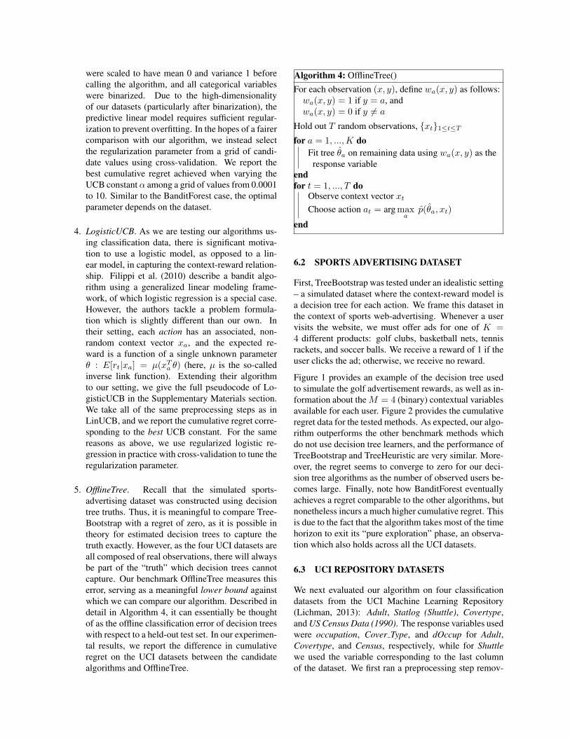
5. OfflineTree. Recall that the simulated sports-advertising dataset was constructed using decisiontree truths. Thus, it is meaningful to compare Tree-Bootstrap with a regret of zero, as it is possible intheory for estimated decision trees to capture thetruth exactly. However, as the four UCI datasets areall composed of real observations, there will alwaysbe part of the “truth” which decision trees cannotcapture. Our benchmark OfflineTree measures thiserror, serving as a meaningful lower bound againstwhich we can compare our algorithm. Described indetail in Algorithm 4, it can essentially be thoughtof as the offline classification error of decision treeswith respect to a held-out test set. In our experimen-tal results, we report the difference in cumulativeregret on the UCI datasets between the candidatealgorithms and OfflineTree.

Algorithm 4: OfflineTree()For each observation (x, y), define wa(x, y) as follows:wa(x, y) = 1 if y = a, andwa(x, y) = 0 if y 6= a

Hold out T random observations, {xt}1≤t≤Tfor a = 1, ...,K do

Fit tree θa on remaining data using wa(x, y) as theresponse variable

endfor t = 1, ..., T do

Observe context vector xtChoose action at = argmax

ap(θa, xt)

end

6.2 SPORTS ADVERTISING DATASET

First, TreeBootstrap was tested under an idealistic setting– a simulated dataset where the context-reward model isa decision tree for each action. We frame this dataset inthe context of sports web-advertising. Whenever a uservisits the website, we must offer ads for one of K =4 different products: golf clubs, basketball nets, tennisrackets, and soccer balls. We receive a reward of 1 if theuser clicks the ad; otherwise, we receive no reward.

Figure 1 provides an example of the decision tree usedto simulate the golf advertisement rewards, as well as in-formation about theM = 4 (binary) contextual variablesavailable for each user. Figure 2 provides the cumulativeregret data for the tested methods. As expected, our algo-rithm outperforms the other benchmark methods whichdo not use decision tree learners, and the performance ofTreeBootstrap and TreeHeuristic are very similar. More-over, the regret seems to converge to zero for our deci-sion tree algorithms as the number of observed users be-comes large. Finally, note how BanditForest eventuallyachieves a regret comparable to the other algorithms, butnonetheless incurs a much higher cumulative regret. Thisis due to the fact that the algorithm takes most of the timehorizon to exit its “pure exploration” phase, an observa-tion which also holds across all the UCI datasets.

6.3 UCI REPOSITORY DATASETS

We next evaluated our algorithm on four classificationdatasets from the UCI Machine Learning Repository(Lichman, 2013): Adult, Statlog (Shuttle), Covertype,and US Census Data (1990). The response variables usedwere occupation, Cover Type, and dOccup for Adult,Covertype, and Census, respectively, while for Shuttlewe used the variable corresponding to the last columnof the dataset. We first ran a preprocessing step remov-

0 20000 40000 60000 80000 100000

020

0040

0060

0080

0010

000

Sample Time

Cum

ulat

ive

Reg

ret

Context−Free MABBandit ForestLinUCBLogisticUCBTreeBootstrapTreeHeuristic

Context−Free MABBanditForestLinUCBLogisticUCBTreeBootstrapTreeHeuristic

Figure 2: Cumulative regret incurred on the (simulated)sports advertising dataset.

ing classes which were significantly underrepresented ineach dataset (i.e., less than 0.05% of the observations).After preprocessing, these datasets had K = 12, 4, 7,and 9 classes, respectively, as well as M = 14, 9, 54,and 67 contextual variables. We then constructed a ban-dit problem from the data in the following way: a regretof 0 (otherwise 1) is incurred if and only if the algorithmpredicts the class of the data point correctly. This frame-work for adapting classification data for use in banditproblems is commonly used in the literature (Allesiardoet al., 2014; Agarwal et al., 2014; Feraud et al., 2016).

Figure 4 shows the cumulative regret of TreeBootstrapcompared with the benchmarks on the UCI datasets. Re-call that we plot regret relative to OfflineTree. In allcases, our heuristic achieves a performance equal to orbetter than that of TreeBootstrap. Note that LogisticUCBoutperforms LinUCB on all datasets except Covertype,which demonstrates the value of using learners in our set-ting which handle binary response data effectively.

LinUCB and LogisticUCB outperform our algorithm ontwo of the four UCI datasets (Adult and Census). How-ever, there are several caveats to this result. First, re-call that we only report the cumulative regret of Lin-UCB and LogisticUCB with respect to the best explo-ration parameter, which is impossible to know a priori.Figure 3 shows LinUCB’s cumulative regret curves cor-responding to each value of the exploration parameter αimplemented on the Adult dataset. We overlay this ona plot of the cumulative regret curves associated withTreeBootstrap and our heuristic. Note that TreeBoot-strap and TreeHeuristic outperformed LinUCB in at leasthalf of the parameter settings attempted. Second, the

difference in cumulative regret between TreeBootstrapand Linear/Logistic UCB on Adult and Census appearsto approach a constant as the time horizon increases.This is due to the fact that decision trees will capturethe truth eventually given enough training data. Con-versely, in settings such as the sports ad dataset, Cover-type, and Shuttle, it appears that the linear/logistic regres-sion models have already converged and fail to capturethe context-reward distribution accurately. This is mostlikely due to the fact that feature engineering is neededfor the data to satisfy the GLM framework. Thus, thedifference in cumulative regret between Linear/LogisticUCB and TreeBootstrap will become arbitrarily large asthe time horizon increases. Finally, note that we intro-duce regularization into the linear and logistic regres-sions, tuned using cross-validation, which improve uponthe original framework for LinUCB and Logistic UCB.

0 10000 20000 30000 40000 50000

020

0040

0060

0080

00

Sample Time

Cum

ulat

ive

Reg

ret −

Offl

ineT

ree

LinUCBTreeBootstrapTreeHeuristic

Figure 3: Cumulative regret incurred on the Adultdataset. The performance of LinUCB is given with re-spect to all values of the tuneable parameter attempted:α = 0.0001, 0.001, 0.01, 0.1, 1, 10

7 CONCLUSION

We propose a contextual bandit algorithm, TreeBoot-strap, which can be easily and effectively applied in prac-tice. We use decision trees as our base learner, and wehandle the exploration-exploitation trade-off using boot-strapping in a way which approximates the behavior ofThompson sampling. As our algorithm requires fittingmultiple trees at each time step, we provide a computa-tional heuristic which works well in practice. Empiri-cally, our methods’ performance is quite competitive androbust compared to several well-known algorithms.

0 10000 20000 30000 40000 50000

020

0040

0060

0080

0010

000

Sample Time

Cum

ulat

ive

Reg

ret −

Offl

ineT

ree

Context−Free MABBandit ForestLinUCBLogisticUCBTreeBootstrapTreeHeuristic

Context−Free MABBanditForestLinUCBLogisticUCBTreeBootstrapTreeHeuristic

(a) Adult Dataset Results

0 10000 20000 30000 40000 50000

020

0040

0060

0080

0010

000

Sample Time

Cum

ulat

ive

Reg

ret −

Offl

ineT

ree

Context−Free MABBandit ForestLinUCBLogisticUCBTreeBootstrapTreeHeuristic

Context−Free MABBanditForestLinUCBLogisticUCBTreeBootstrapTreeHeuristic

(b) Statlog (Shuttle) Dataset Results

0 20000 40000 60000 80000 100000

010

000

2000

030

000

4000

0

Sample Time

Cum

ulat

ive

Reg

ret −

Offl

ineT

ree

Context−Free MABBandit ForestLinUCBLogisticUCBTreeBootstrapTreeHeuristic

Context−Free MABBanditForestLinUCBLogisticUCBTreeBootstrapTreeHeuristic

(c) Covertype Dataset Results

0 20000 40000 60000 80000 100000

050

0010

000

2000

030

000

Sample Time

Cum

ulat

ive

Reg

ret −

Offl

ineT

ree

Context−Free MABBandit ForestLinUCBLogisticUCBTreeBootstrapTreeHeuristic

Context−Free MABBanditForestLinUCBLogisticUCBTreeBootstrapTreeHeuristic

(d) Census Dataset Results

Figure 4: Cumulative regret incurred on various classification datasets from the UCI Machine Learning Repository. Aregret of 0 (otherwise 1) is incurred iff a candidate algorithm predicts the class of the data point correctly.

ReferencesAbbasi-Yadkori, Y., Pal, D., and Szepesvari, C. (2011).

Improved algorithms for linear stochastic bandits. InAdvances in Neural Information Processing Systems,pages 2312–2320.

Agarwal, A., Hsu, D., Kale, S., Langford, J., Li, L., andSchapire, R. (2014). Taming the monster: A fast andsimple algorithm for contextual bandits. In Proceed-ings of The 31st International Conference on MachineLearning, pages 1638–1646.

Agrawal, S. and Goyal, N. (2013). Thompson samplingfor contextual bandits with linear payoffs. In ICML(3), pages 127–135.

Allesiardo, R., Feraud, R., and Bouneffouf, D. (2014).A neural networks committee for the contextual ban-dit problem. In International Conference on NeuralInformation Processing, pages 374–381. Springer.

Auer, P. (2002). Using confidence bounds forexploitation-exploration trade-offs. Journal of Ma-chine Learning Research, 3(Nov):397–422.

Baransi, A., Maillard, O.-A., and Mannor, S. (2014).Sub-sampling for multi-armed bandits. In JointEuropean Conference on Machine Learning andKnowledge Discovery in Databases, pages 115–131.Springer.

Breiman, L., Friedman, J., Stone, C. J., and Olshen,R. A. (1984). Classification and regression trees. CRCpress.

Chu, W., Li, L., Reyzin, L., and Schapire, R. E. (2011).Contextual bandits with linear payoff functions. InAISTATS, volume 15, pages 208–214.

Crawford, S. L. (1989). Extensions to the cart algo-rithm. International Journal of Man-Machine Studies,31(2):197–217.

Dhar, S. and Varshney, U. (2011). Challenges and busi-ness models for mobile location-based services andadvertising. Communications of the ACM, 54(5):121–128.

Dudik, M., Hsu, D., Kale, S., Karampatziakis, N., Lang-ford, J., Reyzin, L., and Zhang, T. (2011). Efficientoptimal learning for contextual bandits. arXiv preprintarXiv:1106.2369.

Eckles, D. and Kaptein, M. (2014). Thompson sam-pling with the online bootstrap. arXiv preprintarXiv:1410.4009.

Feraud, R., Allesiardo, R., Urvoy, T., and Clerot, F.(2016). Random forest for the contextual bandit prob-lem. In Proceedings of the 19th International Con-ference on Artificial Intelligence and Statistics, pages93–101.

Filippi, S., Cappe, O., Garivier, A., and Szepesvari, C.(2010). Parametric bandits: The generalized linearcase. In Advances in Neural Information ProcessingSystems, pages 586–594.

Friedman, J., Hastie, T., and Tibshirani, R. (2001). Theelements of statistical learning, volume 1. Springerseries in statistics Springer, Berlin.

Kim, E. S., Herbst, R. S., Wistuba, I. I., Lee, J. J., Blu-menschein, G. R., Tsao, A., Stewart, D. J., Hicks,M. E., Erasmus, J., Gupta, S., et al. (2011). The battletrial: personalizing therapy for lung cancer. Cancerdiscovery, 1(1):44–53.

Langford, J. and Zhang, T. (2008). The epoch-greedyalgorithm for multi-armed bandits with side informa-tion. In Advances in neural information processingsystems, pages 817–824.

Li, L., Chu, W., Langford, J., Moon, T., and Wang, X.(2011). An unbiased offline evaluation of contextualbandit algorithms with generalized linear models.

Li, L., Chu, W., Langford, J., and Schapire, R. E. (2010).A contextual-bandit approach to personalized news ar-ticle recommendation. In Proceedings of the 19th in-ternational conference on World wide web, pages 661–670. ACM.

Lichman, M. (2013). UCI machine learning repository.

Long, J. S. (1997). Regression models for categoricaland limited dependent variables. Advanced quantita-tive techniques in the social sciences, 7.

Osband, I. and Van Roy, B. (2015). Bootstrapped thomp-son sampling and deep exploration. arXiv preprintarXiv:1507.00300.

Russo, D. and Van Roy, B. (2014). Learning to opti-mize via posterior sampling. Mathematics of Opera-tions Research, 39(4):1221–1243.

Tang, L., Jiang, Y., Li, L., Zeng, C., and Li, T. (2015).Personalized recommendation via parameter-free con-textual bandits. In Proceedings of the 38th Interna-tional ACM SIGIR Conference on Research and De-velopment in Information Retrieval, pages 323–332.ACM.

Utgoff, P. E. (1989). Incremental induction of decisiontrees. Machine learning, 4(2):161–186.

Utgoff, P. E., Berkman, N. C., and Clouse, J. A. (1997).Decision tree induction based on efficient tree restruc-turing. Machine Learning, 29(1):5–44.

Yuan, S.-T. and Tsao, Y. W. (2003). A recommendationmechanism for contextualized mobile advertising. Ex-pert Systems with Applications, 24(4):399–414.