A PRACTICAL FACTORIZATION OF A SCHUR … · a practical factorization of a schur complement for...
22
A PRACTICAL FACTORIZATION OF A SCHUR COMPLEMENT FOR PDE-CONSTRAINED DISTRIBUTED OPTIMAL CONTROL * YOUNGSOO CHOI † , CHARBEL FARHAT ‡ , WALTER MURRAY § , AND MICHAEL SAUNDERS ¶ Abstract. A distributed optimal control problem with the constraint of a linear elliptic partial differential equation is considered. A necessary optimality condition for this problem forms a saddle point system, the efficient and accurate solution of which is crucial. A new factorization of the Schur complement for such a system is proposed and its characteristics discussed. The factorization introduces two complex factors that are complex conjugate to each other. The proposed solution methodology involves the application of a parallel linear domain decomposition solver—FETI-DPH— for the solution of the subproblems with the complex factors. Numerical properties of FETI-DPH in this context are demonstrated, including numerical and parallel scalability and regularization dependence. The new factorization can be used to solve Schur complement systems arising in both range-space and full-space formulations. In both cases, numerical results indicate that the complex factorization is promising. Especially, in the full-space method with the new factorization, the number of iterations required for convergence is independent of regularization parameter values. Key words. PDE-constrained optimization, Schur complement, Poisson operator, FETI, range- space method, full-space method, distributed optimal control AMS subject classifications. 65N22, 65N55, 65F10, 65F50 1. Introduction. Numerical methods for solving partial differential equations (PDEs) have broad applications in the simulation of complicated physical models, the prediction of their response, and design. An important and practical subset of these applications—particularly for design—involves the use of a mathematical optimization technique in which the PDE takes the role of a constraint equation. Two methodologies for PDE-constrained optimization problems are SAND (simultaneous analysis and design) and NAND (nested analysis and design) [3]. NAND uses PDEs to express decision variables as an implicit function of state variables and does not include state variables as optimization variables. Thus, the size of the optimization problem is not typically large. On the other hand, the SAND approach takes both decision variables and state variables as optimization variables and considers PDEs to be equality constraints. Consequently, the size of the system in the SAND approach is generally much larger. The NAND approach has traditionally been the method of choice for physics-based applications not only because SAND requires the solution of a large-scale system of equations but also because NAND conveniently permits the direct use of existing solvers for both optimization and PDE simulation as a black box. However, NAND suffers from the fact that many PDE simulations are required for function evaluations—typically the most expensive part of this approach. Due to the continuous increase in computational power (e.g., speed of processing, capacity of memory, high performance computing) accompanied by the development of robust and versatile numerical algorithms (e.g., parallel algorithms), the SAND approach * The first and second authors acknowledge partial support by the Army Research Laboratory through the Army High Performance Computing Research Center under Cooperative Agreement W911NF-07-2-0027. The third and fourth authors acknowledge partial support by the ONR grant N000141110067. † Aeronautics and Astronautics, Stanford University, Stanford, CA, USA ‡ Aeronautics and Astronautics, Mechanical Engineering, Stanford University, Stanford, CA, USA § Management Science and Engineering, Stanford University, Stanford, CA, USA ¶ Management Science and Engineering, Stanford University, Stanford, CA, USA 1
Transcript of A PRACTICAL FACTORIZATION OF A SCHUR … · a practical factorization of a schur complement for...
A PRACTICAL FACTORIZATION OF A SCHUR COMPLEMENTFOR PDE-CONSTRAINED DISTRIBUTED OPTIMAL CONTROL∗
YOUNGSOO CHOI† , CHARBEL FARHAT‡ , WALTER MURRAY§ , AND MICHAEL
SAUNDERS¶
Abstract. A distributed optimal control problem with the constraint of a linear elliptic partialdifferential equation is considered. A necessary optimality condition for this problem forms a saddlepoint system, the efficient and accurate solution of which is crucial. A new factorization of theSchur complement for such a system is proposed and its characteristics discussed. The factorizationintroduces two complex factors that are complex conjugate to each other. The proposed solutionmethodology involves the application of a parallel linear domain decomposition solver—FETI-DPH—for the solution of the subproblems with the complex factors. Numerical properties of FETI-DPHin this context are demonstrated, including numerical and parallel scalability and regularizationdependence. The new factorization can be used to solve Schur complement systems arising in bothrange-space and full-space formulations. In both cases, numerical results indicate that the complexfactorization is promising. Especially, in the full-space method with the new factorization, thenumber of iterations required for convergence is independent of regularization parameter values.
Key words. PDE-constrained optimization, Schur complement, Poisson operator, FETI, range-space method, full-space method, distributed optimal control
AMS subject classifications. 65N22, 65N55, 65F10, 65F50
1. Introduction. Numerical methods for solving partial differential equations(PDEs) have broad applications in the simulation of complicated physical models,the prediction of their response, and design. An important and practical subsetof these applications—particularly for design—involves the use of a mathematicaloptimization technique in which the PDE takes the role of a constraint equation. Twomethodologies for PDE-constrained optimization problems are SAND (simultaneousanalysis and design) and NAND (nested analysis and design) [3]. NAND uses PDEsto express decision variables as an implicit function of state variables and does notinclude state variables as optimization variables. Thus, the size of the optimizationproblem is not typically large. On the other hand, the SAND approach takes bothdecision variables and state variables as optimization variables and considers PDEs tobe equality constraints. Consequently, the size of the system in the SAND approachis generally much larger. The NAND approach has traditionally been the method ofchoice for physics-based applications not only because SAND requires the solution ofa large-scale system of equations but also because NAND conveniently permits thedirect use of existing solvers for both optimization and PDE simulation as a blackbox. However, NAND suffers from the fact that many PDE simulations are requiredfor function evaluations—typically the most expensive part of this approach. Due tothe continuous increase in computational power (e.g., speed of processing, capacityof memory, high performance computing) accompanied by the development of robustand versatile numerical algorithms (e.g., parallel algorithms), the SAND approach
∗The first and second authors acknowledge partial support by the Army Research Laboratorythrough the Army High Performance Computing Research Center under Cooperative AgreementW911NF-07-2-0027. The third and fourth authors acknowledge partial support by the ONR grantN000141110067.†Aeronautics and Astronautics, Stanford University, Stanford, CA, USA‡Aeronautics and Astronautics, Mechanical Engineering, Stanford University, Stanford, CA, USA§Management Science and Engineering, Stanford University, Stanford, CA, USA¶Management Science and Engineering, Stanford University, Stanford, CA, USA
1
2 Y. CHOI, C. FARHAT, W. MURRAY, AND M. SAUNDERS
has received increasing attention from researchers in recent years [4, 5, 7, 31], and thepresent study continues this line of research.
The SAND approach to PDE-constrained optimization takes the form
minimizey,u
F (y, u)
subject to C(y, u) = 0,(1.1)
where C(y, u) = 0 is the time-independent PDE constraint, y is the vector of statevariables, and u is the vector of decision variables. State variables by definition are theunknown variables in the forward PDE problem. For example, state variables comprisetemperature in heat conduction problems and displacements in elastostatics. For theclass of PDE-constrained optimization known as optimal control the decision variablesu are referred to as control variables, whereas for optimal design or shape optimizationproblems the decision variables u are called design variables. The decision variablesmay also be a set of parameters describing the material properties or the system ofdynamics for some inverse problems. All three types of PDE-constrained optimizationproblems share a similar structure of their linear or linearized system of equationsknown as a KKT system, after the Karush-Kuhn-Tucker optimality conditions, or asaddle point system.
In what follows, a robust and versatile numerical method for solving a distributedoptimal control problem is considered. In particular, heat conduction and elastostaticPDE-constrained problems are studied, although the method developed here can alsobe applied or extended easily to other types of PDE-constrained optimization prob-lems. From various possible objective functions that may be used to formulate adistributed PDE-constrained optimal control problem, the one considered is that inwhich a target state is assumed to be given. Thus, the aim is to find a state thatis close to the prescribed target and a control that realizes that particular state.For example, the static thermal conduction optimal control problem with a targettemperature distribution y is formulated as
minimizey,u
F (y, u) :=1
2
∫Ω
(y − y)2dx+φ
2
∫Ω
u2dx
subject to −∇2y = u on Ω
y = yc on Γg.
(1.2)
The solution of this problem is considered in Section 6.1. Variables y and u are thetemperature state and heat source control, respectively, while yc is the prescribedboundary conditions and φ is a regularization parameter. The domain of interest isdenoted as Ω and a Dirichlet boundary condition is imposed on the boundary Γg.Note that a unit conductivity is assumed.
Two alternative approaches to PDE-constrained optimization problems such as(1.2) are optimize-and-discretize and discretize-and-optimize. The latter approach,in which one first discretizes both the objective function and constraints and thenobtains the discretized optimality condition, is typically used for PDE-constrainedoptimal control [5, 9, 30, 29, 32, 35, 11] and is followed here.
Solving the saddle point system representing the discretized optimality conditionefficiently is crucial to the competitiveness of the SAND approach, in comparison withNAND. There are two methodologies for solving a saddle point system.
• In reduced-space methods, one attempts to reduce the size of a saddle pointsystem by eliminating some variables and solving a smaller system [37, 38,
A PRACTICAL FACTORIZATION OF THE SCHUR COMPLEMENT 3
35, 4]. The range-space method and the null-space method are two popularreduced-space methods. In the range-space method, one solves for the dualvariables first using the corresponding Schur complement and subsequentlyupdates the primal variables, whereas the null-space method subdivides thevariables algebraically into null-space variables and range-space variables us-ing null-space and range-space bases of the constraint Jacobian.
• In full-space methods, one solves for the primal and dual variables simulta-neously. The resultant system of equations becomes a sparse saddle pointsystem and iterative methods are the only practical choice for large prob-lems. Various efficient preconditioners for saddle point systems have beendeveloped [27, 2, 22, 16, 32, 30, 10, 9, 23, 5, 36]. However, there is still mo-tivation for further research in this area. For example, most preconditionersare not robust when φ is small. Recently, Pearson and Wathen have devel-oped a new approximation of the Schur complement and used it to facilitatea regularization-robust preconditioner for a particular distributed optimalcontrol problem [30]. Pearson et al. have further extended the usage of theaforementioned approximation to a broader range of optimal control problems[29].
The factorization of the Schur complement presented in this paper has a similarform to Pearson and Wathen’s approximation, and furthermore is applied to the sameparticular distributed optimal control problem [30]. However the approach taken herediffers from that of Pearson and Wathen in two ways. First and foremost, becausethe factorization is exact by its nature, the range-space method can be adopted andone efficient solve with the Schur complement results in a solution to the distributedoptimal control problem. Second, a scalable domain decomposition based parallellinear solver FETI-DPH [13] is used to solve each of the subproblems arising in theapplication of the proposed factorization. In contrast, Pearson and Wathen suggest amultigrid method.
The outline of the paper is as follows: Section 2 describes discretization of thedistributed optimal control problem (1.2) and the corresponding optimality condition,which is a saddle point system. Section 3 outlines two methods for solving the saddlepoint system: the range-space method and the full-space method. Additionally, thissection reviews existing preconditioners for the full-space method related to the Schurcomplement in the range-space method. Section 4 introduces a practical factorizationof the Schur complement and explains how it can be used in both the range-spacemethod and the full-space method. Section 5 describes the Finite Element Tearingand Interconnecting (FETI) method and its so-called dual-primal variants, FETI-DPand FETI-DPH. Section 6 presents numerical results that illustrate the scalability andefficiency of the method applied to a selection of distributed optimal control problems.
2. Distributed control problems. In this section, the finite element discretiza-tion of a distributed optimal control problem is introduced and the correspondingoptimality condition is presented. For brevity, we choose to show the discretization ofa distributed optimal control problem with a constraint of the Poisson equation (i.e.,Eq. (1.2)). However, distributed optimal control problems with other types of PDEconstraints (e.g., linear elasticity) will have the same discretized formulation. The
4 Y. CHOI, C. FARHAT, W. MURRAY, AND M. SAUNDERS
finite element discretization of (1.2) gives
minimizey,u
F (y,u) :=1
2‖y − y‖2V +
φ
2‖u‖2V
subject to Ky + Kcyc = Vu,
(2.1)
where K, V ∈ Rn×n, and Kc ∈ Rn×m are the stiffness matrix, volume matrix, andconstrained stiffness matrix, respectively. Vector valued quantities y, y, u ∈ Rn,and yc ∈ Rm are the discretized versions of the target state, state, control, andprescribed boundary conditions, respectively. All the discrete variables are denotedwith bold fonts for the remainder of the paper. The dimensions n and m are thenumber of unconstrained degrees of freedom (i.e., the size of y) and the number ofconstrained degrees of freedom, respectively. It is assumed that both K and V aresymmetric positive definite (SPD) matrices, which is the case for the thermal problem
above. The energy norm ‖ · ‖V is defined as ‖q‖V =√qTVq. The details of the
finite element discretization procedure can be found in [7]. Problem (2.1) is a convexquadratic program and its solution is a saddle point of the Lagrangian,
L(y,u,λ) =1
2‖y − y‖2V +
φ
2‖u‖2V + λT (Ky + Kcyc −Vu). (2.2)
A saddle point (y∗,u∗,λ∗) must satisfy the following optimality condition:V 0 K0 φV −VK −V 0
y∗
u∗
λ∗
=
Vy0
−Kcyc
. (2.3)
This equation is of the form Ax = b, where A is a symmetric indefinite matrix.Section 3 explains two ways of solving the saddle point system in (2.3): the range-space method and full-space method.
3. Range-space and full-space methods.
3.1. Range-space method. The range-space method was introduced for large-scale inequality-constrained convex quadratic programming problems with small ac-tive sets in order to overcome the disadvantage of the null-space method: the in-creasingly high dimension of the null space basis as a solution is approached [19, 20].For equality-constrained convex quadratic programming, the range-space method isequivalent to the Schur complement method [37] where the corresponding dual prob-lem is solved first. The range-space method is a reduced-space method in a sense thatthe size of the saddle point system in (2.3) is reduced by eliminating y∗ and u∗ andsolving for λ∗ first. The dual variable λ∗ is obtained by solving
Sλ∗ = Kcyc + Ky, (3.1)
where S = KV−1K + 1φV is known as the negative Schur complement on the dual
variables. Then, y∗ and u∗ are computed from
y∗ = y −V−1Kλ∗ and u∗ =1
φλ∗. (3.2)
The most expensive and crucial step in the range-space method is to solve with S in(3.1). The eigenvalues (and consequently, the condition number) of S depend on those
A PRACTICAL FACTORIZATION OF THE SCHUR COMPLEMENT 5
of K and V and the value of φ [37, 7]. For small values of φ, the condition numberof S is affected most by the eigenvalues of V, whose condition number is boundedabove by a constant, C, for Pq or Qq (the qth order triangular or quadrilateral finiteelements in 2D and tetrahedral or brick elements in 3D) if a set of grids is quasi-uniform (see Eq. (1.116) and Eq. (1.117) in [12]). The constant C depends on theorder of approximation q but not on the mesh size h. Thus for small values of φ, evenif the grid is refined or the problem size is increased, the condition number of S isbounded. For large values of φ, the condition number of S (denoted by κ(S)) dependson κ(KV−1K), which is proportional to κ(K)2. For a second-order elliptic operator,one can prove that κ(K) < ch−2 if Pq or Qq is used on a quasi-uniform discretizationof a domain (see Eq. (1.119) and Eq. (1.121) in [12]). For a higher-order ellipticoperator, the dependence on h of κ(K) increases (e.g., the shell or beam elements).This is unfortunate because κ(K) is likely to increase as the mesh size h decreases orthe problem size increases. One remedy is to apply iterative refinement with a highprecision data type. If the solution is inaccurate even after iterative refinement dueto the ill-conditioning of S, an alternative way of solving (2.3) that avoids an exactsolve with S is to use the full-space method, which is explained in the next section.
An additional challenge in applying the range-space method for solving (2.3)resides in solving with S itself. Because S is a sum of two matrices (KV−1K and1φV), the first of which is a product requiring two matrix-matrix multiplications toevaluate, it is not straightforward to come up with an efficient way of solving withS. In Section 4, a practical factorization of S is introduced and the factorizationdoes not require matrix-matrix products. The factorization introduced in Section 4introduces complex symmetric matrices (not Hermitian matrices) in its factors. Alist of efficient solvers for complex symmetric matrices includes CG-type methods[17], CS-MINRES-QLP [6], GMRES [34, 8], FETI-DPH [13], and multi-grid methods[24, 33]. FETI-DPH is explained in Section 5 and used in numerical experiments inSection 6.
3.2. Full-space Method. The full-space method attempts to solve for all thevariables of the saddle point system in (2.3) simultaneously. As the discretization isrefined, the size of the system becomes large and an iterative method is often theonly available method. Because A is a symmetric indefinite matrix, any Krylov it-erative method suitable for this class of matrices, such as MINRES [28], SYMMLQ[28], SQMR [18], and GMRES, can be used. For successful convergence of the iter-ative method, one is often required to apply a good preconditioner. Even withoutany preconditioner, the saddle point system itself tends to be better conditioned formoderately large values of φ than the Schur complement in the range-space method[37]. If a good preconditioner is used, the full-space method is likely to have a betterscalability than the range-space method, meaning that computational cost does notgrow at an exponential rate as the problem size increases. Thus, many preconditionershave been developed recently. Here we focus on a Schur complement-based precon-ditioner because the primary interest is to discuss the usage of a Schur complementfactorization that will be introduced in Section 4. Murphy, et al. [27] have shown thatif the following block diagonal preconditioner is used, then the preconditioned system
has at most three nonzero distinct eigenvalues (1, 1±√
52 ):
Pmgw =
V 0 00 φV 00 0 S
, (3.3)
6 Y. CHOI, C. FARHAT, W. MURRAY, AND M. SAUNDERS
where S is the negative Schur complement defined in (3.1). This implies that themaximum number of iterations required for convergence in a Krylov iterative methodis three if Pmgw is used as a preconditioner. However, applying this preconditioner haspreviously been considered impractical because it requires solving with S in order toapply Pmgw. Even if it were practical to solve with S efficiently and accurately, thenthe preferred approach would typically be to use the range-space method rather thanto apply Pmgw in the full-space method because the range-space method requires onlyone solve with S, while the full space method with Pmgw as a preconditioner is likelyto require more than one solve with S. There has been some research done on findinga good approximation of the Schur complement for use in a Schur complement-basedpreconditioner (e.g., Pmgw) [32, 30, 29]. Particularly, Pearson and Wathen [30] havedeveloped the following approximation, which is regularization-robust:
Sp = (K +1√φV)V−1(K +
1√φV)
= S +2√φK,
(3.4)
and proved that the eigenvalues of S−1p S are between 1
2 and 1 regardless of the meshsize h and φ. This implies theoretically that a Krylov iterative method must con-verge in O(1) iterations regardless of h and φ. They have used an algebraic multi-
grid method to solve with the factor(K + 1√
φV)
in their numerical examples and
demonstrated that the number of iterations required for convergence is indeed O(1).However, in the problems they solve, the condition number of the Schur complementis small enough so that the approximation to the Schur complement behaves well.The factorization introduced in Section 4 has a similar form to (3.4). However, it isan exact representation of S and therefore enables the application of the range-spacemethod.
4. A “practical” factorization of the Schur complement. The Schur com-plement S in (3.1) can be factored into the following form:
Sc = (K− i√φV)V−1(K +
i√φV), (4.1)
where i =√−1. The form of this factorization is similar to Sp in (3.4) in the sense
that the first and third factors are some linear combinations of K and V, and themiddle factor is V−1. This suggests that the same methods for solving with thefactors in Sp may also be used to solve with factors in Sc. Because Sc is an exactfactorization of S, if Sc is used in Schur complement-based preconditioner, the numberof iterations required for convergence in the full-space method must not depend onvalues of regularization parameter as the ones of the full-space method with Sp-based Schur complement preconditioner does not depend on values of regularizationparameter. However, there are some important differences between Sp and Sc. Thefirst and third factors of Sp are the same, but the corresponding factors of Sc arenot. Consequently, if direct solvers were to be used for each factor, then only onefactorization would be required for Sp, while two factorizations of two different systemswould be required for Sc. Additionally, Sc introduces complex numbers, but all theelements in Sp are real. Thus, one solve with Sc requires four times more storageand floating point operations than one solve with Sp. In spite of the disadvantages ofapplying Sc, it is an exact representation of S, and this permits use of the range-space
A PRACTICAL FACTORIZATION OF THE SCHUR COMPLEMENT 7
method where only one solve with Sc is sufficient to obtain a solution to (2.1). Onthe other hand, several solves with Sp are required because Sp is an approximation toS, so it can only be used as a preconditioner. This discussion leads to the followingtwo extreme cases when dealing with the Schur complement:
• If a direct method is the preferred choice for solving the Schur complement(i.e., a factorization of a given system is required), it would be advantageous toapply the direct method to Sp assuming that the dominating computationalcost occurs in factorization of the system.
• If an iterative method is the only option and the range-space method is ap-plicable, then it would be preferable to apply the iterative method to Sc.
Between these two extreme cases, a choice must be made depending on the character-istics of the problem and a numerical solver. For example, if the domain of a problemis complex, then the computational overhead incurred by applying Sc rather than Spwill be substantially diminished since in this case the factors of both Sc and Sp willbe complex. Such problems include any frequency domain analyses with dampingin structural or acoustic problems. On the other hand, if a problem requires sev-eral solves with a Schur complement and with multiple right-hand sides and is smallenough to permit a direct solver to be used for the factors of S, applying Sp is favor-able because direct methods are more efficient than iterative methods in general formultiple right-hand sides. If a domain decomposition method—in which both directand iterative methods are used—is chosen, then one needs to examine the costs ofeach component of the computation (e.g., data structure, building and storing theoperator, and solving with the operator). In Section 6, numerical results for solvingwith Sc are shown using the domain decomposition solver FETI-DPH [13].
5. FETI. In order to be self-contained, the FETI method [15] and two of itsvariants (FETI-DP [14] and FETI-DPH [13]) are explained in this section. For amore detailed description, see [15, 14, 13, 1]. The FETI method was developed inorder to solve, in parallel, the following linear system of equations arising from thefinite element discretization of a linear elasticity PDE:
Ky = f , (5.1)
where K is the stiffness matrix (or a linear combination of the stiffness matrix andmass matrix), y is the vector of unknown displacements, and f is an external forceterm. Solving (5.1) is equivalent to minimizing a quadratic function:
minimizey
1
2yTKy − yT f . (5.2)
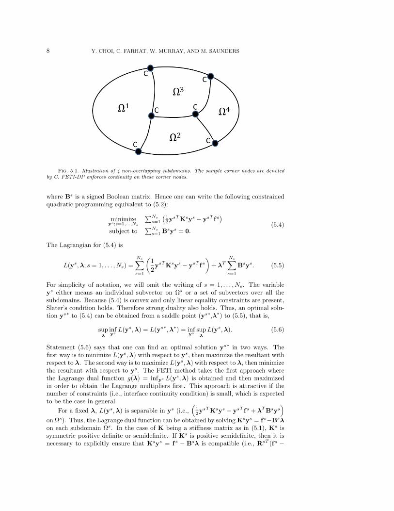
The objective function in (5.2) often represents a physical quantity (e.g., energy inlinear elasticity). In domain decomposition methods, the spatial domain Ω is dividedinto Ns either overlapping or non-overlapping subdomains. The FETI method dividesΩ into Ns non-overlapping subdomains as illustrated in Figure 5.1 and minimizes alocal function in each subdomain (i.e., minimize ysTKsys − ysT fs in Ωs where thesuperscript “s” designate the restrictions to the specific subdomain). In order tobe equivalent to (5.2), the following additional continuity condition on ys betweeninterfaces must be imposed:
Ns∑s=1
Bsys = 0, (5.3)
8 Y. CHOI, C. FARHAT, W. MURRAY, AND M. SAUNDERS
Fig. 5.1. Illustration of 4 non-overlapping subdomains. The sample corner nodes are denotedby C. FETI-DP enforces continuity on these corner nodes.
where Bs is a signed Boolean matrix. Hence one can write the following constrainedquadratic programming equivalent to (5.2):
minimizeys;s=1,...,Ns
∑Ns
s=1
(12y
sTKsys − ysT fs)
subject to∑Ns
s=1 Bsys = 0.
(5.4)
The Lagrangian for (5.4) is
L(ys,λ; s = 1, . . . , Ns) =
Ns∑s=1
(1
2ysTKsys − ysT fs
)+ λT
Ns∑s=1
Bsys. (5.5)
For simplicity of notation, we will omit the writing of s = 1, . . . , Ns. The variableys either means an individual subvector on Ωs or a set of subvectors over all thesubdomains. Because (5.4) is convex and only linear equality constraints are present,Slater’s condition holds. Therefore strong duality also holds. Thus, an optimal solu-tion ys∗ to (5.4) can be obtained from a saddle point (ys∗,λ∗) to (5.5), that is,
supλ
infysL(ys,λ) = L(ys∗,λ∗) = inf
yssupλL(ys,λ). (5.6)
Statement (5.6) says that one can find an optimal solution ys∗ in two ways. Thefirst way is to minimize L(ys,λ) with respect to ys, then maximize the resultant withrespect to λ. The second way is to maximize L(ys,λ) with respect to λ, then minimizethe resultant with respect to ys. The FETI method takes the first approach wherethe Lagrange dual function g(λ) = infys L(ys,λ) is obtained and then maximizedin order to obtain the Lagrange multipliers first. This approach is attractive if thenumber of constraints (i.e., interface continuity condition) is small, which is expectedto be the case in general.
For a fixed λ, L(ys,λ) is separable in ys (i.e.,(
12y
sTKsys − ysT fs + λTBsys)
on Ωs). Thus, the Lagrange dual function can be obtained by solving Ksys = fs−Bsλon each subdomain Ωs. In the case of K being a stiffness matrix as in (5.1), Ks issymmetric positive definite or semidefinite. If Ks is positive semidefinite, then it isnecessary to explicitly ensure that Ksys = fs − Bsλ is compatible (i.e., RsT (fs −
A PRACTICAL FACTORIZATION OF THE SCHUR COMPLEMENT 9
BsTλ) = 0 where the columns of Rs span the left null space of Ks). Otherwise, the
minimum of(
12y
sTKsys − ysT fs + λTBsys)
in terms of ys becomes −∞ and the
objective value of primal problem (5.4) is also −∞ by strong duality. However, thisis not a physical solution. Thus, we restrict ourselves to the case when g(λ) > −∞.Finally, the Lagrange dual function g(λ) = infys L(ys,λ) is defined as
g(λ) =
− 1
2λTFλ + dTλ− c if RsT (fs −BsTλ) = 0 for ∀s,
−∞ otherwise,(5.7)
where
F =
Ns∑s=1
BsKs+BsT , d =
Ns∑s=1
BsKs+fs, c =1
2
Ns∑s=1
fsTKs+fs, (5.8)
and Ks+ is a pseudo-inverse of Ks. This defines the following dual problem to (5.4):
maximizeλ
− 12λ
TFλ + dTλ
subject to RsT (fs −BsTλ) = 0 for ∀s.(5.9)
The FETI method solves (5.9) with a Preconditioned Conjugate Projected Gradient(PCPG) algorithm. The FETI formulation above is suitable for parallel processing.Any subdomain level computations (e.g., factorization or computation with Ks andfs) can be assigned to an individual process. The size of λ is the total number ofdegrees of freedom restricted to the interfaces between subdomains. Within PCPG,λ is projected onto the domain of feasibility, which in turn reduces the effectivedimension of the problem. Indeed the FETI method equipped with the Dirichletpreconditioner is proven numerically scalable with respect to both problem size andnumber of subdomains. The Dirichlet preconditioner is defined as
P−1 = W
Ns∑s=1
Bs
[0 00 Ssbb
]BsTW, (5.10)
where
W =
(Ns∑s=1
BsBsT
)+
, Ssbb = Ksbb −Ks
ibTKs
ii−1Ks
ib, (5.11)
and the subscript i and b denote subdomain internal degrees of freedom and interfacedegrees of freedom, respectively. If it is applied in the conjugate gradient algorithmwith the projected gradient [21] to second-order elliptic problems, the condition num-ber κ of the interface problem (5.9) is approximately [26]
κ = O(1 + logm(H/h)), m ≤ 3. (5.12)
However, the first-generation FETI method is not numerically scalable for fourth-order plate and shell problems. This leads to FETI-DP. FETI-DP is one variantconsidered to be the third-generation FETI method. FETI-DP enforces continuity atsome interface corner nodes at each iteration (see Figure 5.1). An extra coarse problemneeds to be solved [14] and in each subdomain the remaining subdomain stiffnessmatrix Ks
rr (i.e., that excluding the degrees of freedom in the corner nodes at which
10 Y. CHOI, C. FARHAT, W. MURRAY, AND M. SAUNDERS
the continuity is enforced) becomes positive definite. Consequently, the correspondingdual interface problem becomes an unconstrained QP. This treatment helps to achievenumerical scalability for fourth-order elliptic problems. The continuity constraintscan be augmented by additional constraints that are enforced exactly throughout theiterations in FETI-DP in order to accelerate the convergence. This augmentationprocedure results in the augmented coarse problem in FETI-DP [25]. A standardaugmentation procedure uses the edge-based rigid body modes (rotational and/ortranslational) [13]. The positive definiteness of Ks
rr is not guaranteed when K in(5.1) is different from the stiffness matrix. For example, for a Helmholtz problem orfrequency response elastodynamic problem, K in (5.1) becomes
Z ≡ K− k2M + iC, (5.13)
where C is a symmetric matrix that arises from the discretization of an absorbingboundary condition, and k > 0 is a frequency (or a wave number for acoustic scatteringproblems). In this case, depending on the value of k, Z may become indefinite. Thesame difficulty is encountered when solving with complex factors in (4.1). In order toresolve this difficulty, two special treatments were required.
• The first treatment is required to deal with indefinite matrices. A solver thatis suitable for indefinite matrices must be applied. Such an iterative solverincludes GMRES [34] for a general square matrix and MINRES [28] for asymmetric indefinite matrix. FETI-DPH (‘H’ stands for Helmholtz) [13] usesGMRES to deal with indefiniteness.
• The second treatment is required for improved convergence when the wavenumber of frequency is large. A particular augmentation used in FETI-DPHthat accelerates convergence for the Helmholtz or frequency response elasto-dynamic problem is the free-space solutions of the corresponding equations,which are plane waves.
Note that the complex factors in Section 4.1 are similar to (5.13), but not identical,and not surprisingly the plane wave augmentation was found to not provide the samebeneficial effects as in the Helmholtz problem. Thus, the edge-based rigid body modes(both rotational and translational) augmentation is applied in the next section for twonumerical examples. Strictly speaking, although FETI-DPH normally refers to thevariant of FETI-DP that uses both GMRES and plane wave augmentation, in whatfollows, FETI-DPH refers to a FETI-DP solver incorporating GMRES and edge-basedrigid body modes.
6. Numerical Results. Two pedagogical examples are considered: linear staticheat control of a 2D square plate and structure control of a 3D solid cantilever. Theheat control problem in Section 6.1 is taken identical to the thermal problem solvedin the paper by Rees et al. [32]. The Schur complement that arises in this thermalproblem is sufficiently well-conditioned for the range of φ values and mesh size hconsidered here for the range-space method to be applicable and therefore it is theonly method used. The cantilever control problem in Section 6.2 is very flexiblewith material properties of rubber. For a relatively large φ value, the range-spacemethod fails to converge to an accurate solution. Thus, the range-space method isused for small values of φ only, and the full-space method is used for large valuesof φ. In the case of the full-space method, both the approximate Schur complementproposed by Pearson and Wathen [30] and the complex factorization introduced inthis paper are used in a Schur-complement based preconditioner and compared interms of computational time and iteration counts.
A PRACTICAL FACTORIZATION OF THE SCHUR COMPLEMENT 11
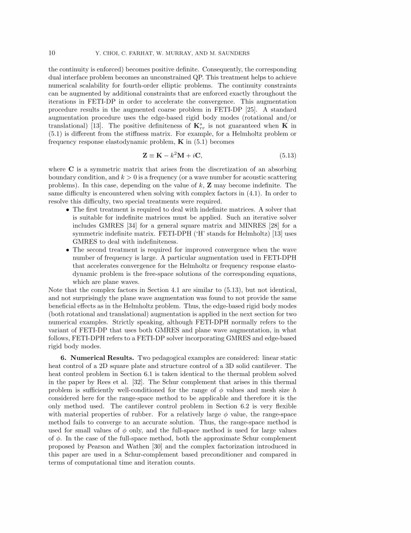
Fig. 6.1. Target temperature defined as in (6.2).
It is well established that augmentation is a beneficial feature that improves theperformance of FETI. However, the optimality of the augmentation’s performancedepends on the nature of the problem. Because neither the FETI solver nor any ofits variants has ever been applied to a system of the form K ± i√
φV, the numerical
performance of FETI-DPH with and without augmentation is compared in this sec-tion. All the simulations were run on a heterogeneous Linux cluster with 2.6 GHzhexa-core Westmere processors (32 blades, 2 processors per blade, QDR Infinibandinterconnect, 24GB/blade) and 2.6 GHz octa-core Sandybridge processors (4 blades,2 processors per blade, FDR Infiniband interconnect, 256 GB/node).
6.1. Thermal problem. A linear static heat control problem is solved. Thisexample is identical to example 5.1 in [32] by Rees et al. The same objective functionand PDE constraints are used as in (1.2), whose continuous formulation is reproducedhere for better access:
minimizey,u
F (y, u) :=1
2
∫Ω
(y − y)2dx+φ
2
∫Ω
u2dx
subject to −∇2y = u on Ω
y = yc on Γg.
(6.1)
The domain Ω is [0, 1]2 ⊂ R2, which is a unit square plate, whose heat conductivityis unity. The target temperature y is defined as
y =
(2x1 − 1)2(2x2 − 1)2 if (x1, x2) ∈ [0, 1
2 ]2,0 otherwise,
(6.2)
which is illustrated in Figure 6.1. The boundary condition yc is defined as
yc = y on Γg = ∂Ω = (x1, x2) | x1 ∈ 0, 1, x2 ∈ 0, 1. (6.3)
The optimal control problem (6.1) tries to find a temperature y that is close to thetarget temperature y by controlling heat u. How close y can be to y is determinedby the parameter φ. As φ decreases, y is expected to approach y, but ‖u‖ is alsoexpected to increase. This makes sense because the objective function value is not
12 Y. CHOI, C. FARHAT, W. MURRAY, AND M. SAUNDERS
(a) (b)
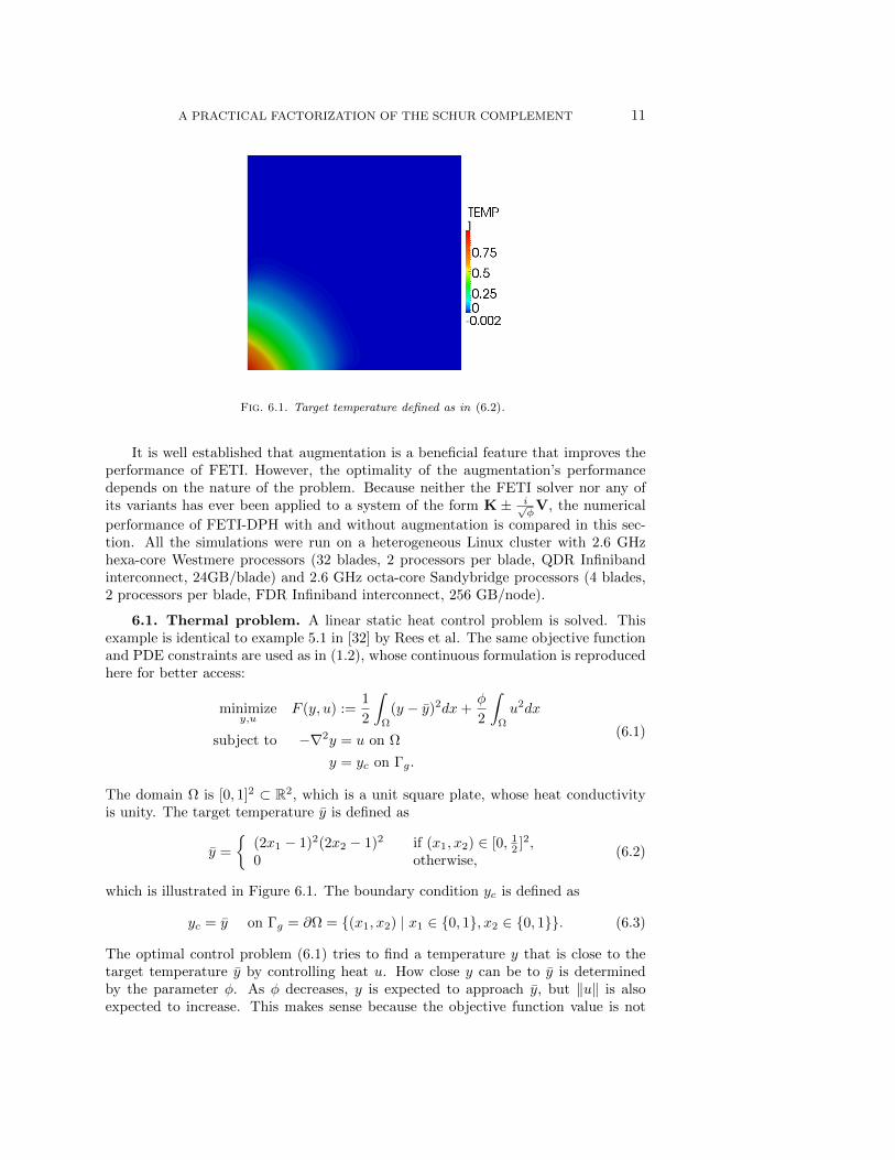
Fig. 6.2. (a) Graph of φ vs relative difference between temperature solution and target temper-ature. (b) Graph of φ vs norm of control solution.
sensitive to the second term if the parameter φ is small and the first term dominatesthe objective function value. The results shown in Figure 6.2 confirm the validityof these expectations. For this particular example, according to Figure 6.2(a), oneneeds φ less than 2 × 10⁻⁶ in order to match the target temperature to within 1%.According to Figure 6.2(b), however, one needs to set φ greater than 2×10⁻⁴ in orderfor the norm of control solution not to exceed 100.
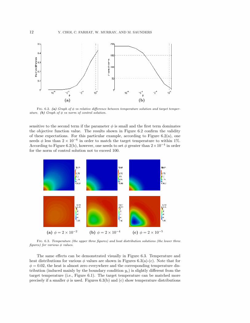
(a) φ = 2× 10⁻² (b) φ = 2× 10⁻⁴ (c) φ = 2× 10⁻⁵
Fig. 6.3. Temperature (the upper three figures) and heat distribution solutions (the lower threefigures) for various φ values.
The same effects can be demonstrated visually in Figure 6.3. Temperature andheat distributions for various φ values are shown in Figures 6.3(a)-(c). Note that forφ = 0.02, the heat is almost zero everywhere and the corresponding temperature dis-tribution (induced mainly by the boundary condition yc) is slightly different from thetarget temperature (i.e., Figure 6.1). The target temperature can be matched moreprecisely if a smaller φ is used. Figures 6.3(b) and (c) show temperature distributions
A PRACTICAL FACTORIZATION OF THE SCHUR COMPLEMENT 13
that are closer to the target temperature. They are produced by using smaller φ val-ues (i.e., φ = 2× 10⁻⁴ and 2× 10⁻⁵). Note that the corresponding heat distributionsshow noticeable non-zero heat at the left bottom of the domain. As φ decreases, asharper heat gradient is visible near the boundary.
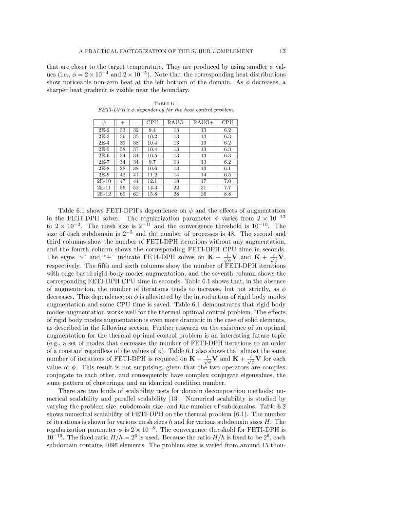
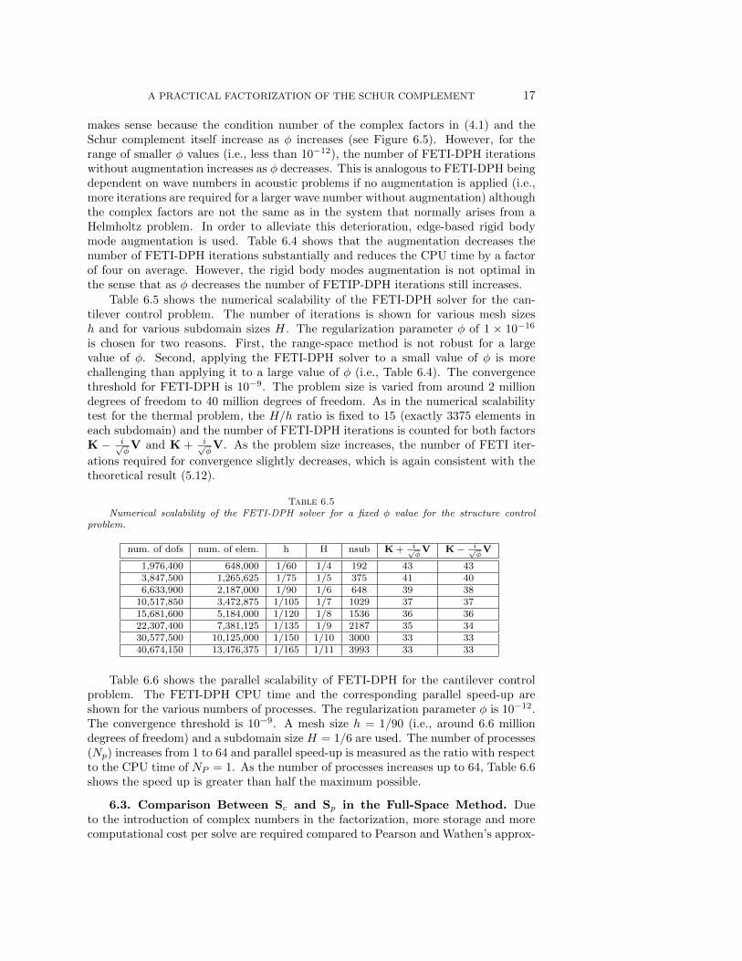
Table 6.1FETI-DPH’s φ dependency for the heat control problem.
φ + - CPU RAUG- RAUG+ CPU
2E-2 33 32 9.4 13 13 6.22E-3 36 35 10.2 13 13 6.32E-4 39 38 10.4 13 13 6.22E-5 38 37 10.4 13 13 6.32E-6 34 34 10.5 13 13 6.32E-7 34 34 9.7 13 13 6.22E-8 38 38 10.6 13 13 6.12E-9 42 41 11.2 14 14 6.52E-10 47 44 12.1 18 17 7.02E-11 56 52 14.3 22 21 7.72E-12 69 62 15.8 28 26 8.8
Table 6.1 shows FETI-DPH’s dependence on φ and the effects of augmentationin the FETI-DPH solver. The regularization parameter φ varies from 2 × 10⁻¹²
to 2 × 10⁻². The mesh size is 2−11 and the convergence threshold is 10−10. Thesize of each subdomain is 2−5 and the number of processes is 48. The second andthird columns show the number of FETI-DPH iterations without any augmentation,and the fourth column shows the corresponding FETI-DPH CPU time in seconds.The signs “-” and “+” indicate FETI-DPH solves on K − i√
φV and K + i√
φV,
respectively. The fifth and sixth columns show the number of FETI-DPH iterationswith edge-based rigid body modes augmentation, and the seventh column shows thecorresponding FETI-DPH CPU time in seconds. Table 6.1 shows that, in the absenceof augmentation, the number of iterations tends to increase, but not strictly, as φdecreases. This dependence on φ is alleviated by the introduction of rigid body modesaugmentation and some CPU time is saved. Table 6.1 demonstrates that rigid bodymodes augmentation works well for the thermal optimal control problem. The effectsof rigid body modes augmentation is even more dramatic in the case of solid elements,as described in the following section. Further research on the existence of an optimalaugmentation for the thermal optimal control problem is an interesting future topic(e.g., a set of modes that decreases the number of FETI-DPH iterations to an orderof a constant regardless of the values of φ). Table 6.1 also shows that almost the samenumber of iterations of FETI-DPH is required on K− i√
φV and K + i√
φV for each
value of φ. This result is not surprising, given that the two operators are complexconjugate to each other, and consequently have complex conjugate eigenvalues, thesame pattern of clusterings, and an identical condition number.
There are two kinds of scalability tests for domain decomposition methods: nu-merical scalability and parallel scalability [13]. Numerical scalability is studied byvarying the problem size, subdomain size, and the number of subdomains. Table 6.2shows numerical scalability of FETI-DPH on the thermal problem (6.1). The numberof iterations is shown for various mesh sizes h and for various subdomain sizes H. Theregularization parameter φ is 2× 10⁻⁸. The convergence threshold for FETI-DPH is10−10. The fixed ratio H/h = 26 is used. Because the ratio H/h is fixed to be 26, eachsubdomain contains 4096 elements. The problem size is varied from around 15 thou-
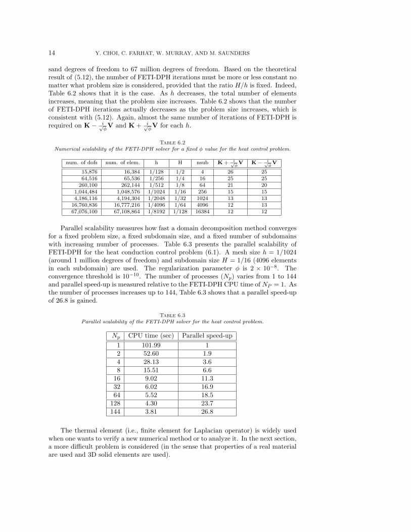
14 Y. CHOI, C. FARHAT, W. MURRAY, AND M. SAUNDERS
sand degrees of freedom to 67 million degrees of freedom. Based on the theoreticalresult of (5.12), the number of FETI-DPH iterations must be more or less constant nomatter what problem size is considered, provided that the ratio H/h is fixed. Indeed,Table 6.2 shows that it is the case. As h decreases, the total number of elementsincreases, meaning that the problem size increases. Table 6.2 shows that the numberof FETI-DPH iterations actually decreases as the problem size increases, which isconsistent with (5.12). Again, almost the same number of iterations of FETI-DPH isrequired on K− i√
φV and K + i√
φV for each h.
Table 6.2Numerical scalability of the FETI-DPH solver for a fixed φ value for the heat control problem.
num. of dofs num. of elem. h H nsub K + i√φ
V K− i√φ
V
15,876 16,384 1/128 1/2 4 26 2564,516 65,536 1/256 1/4 16 25 25
260,100 262,144 1/512 1/8 64 21 201,044,484 1,048,576 1/1024 1/16 256 15 154,186,116 4,194,304 1/2048 1/32 1024 13 13
16,760,836 16,777,216 1/4096 1/64 4096 12 1367,076,100 67,108,864 1/8192 1/128 16384 12 12
Parallel scalability measures how fast a domain decomposition method convergesfor a fixed problem size, a fixed subdomain size, and a fixed number of subdomainswith increasing number of processes. Table 6.3 presents the parallel scalability ofFETI-DPH for the heat conduction control problem (6.1). A mesh size h = 1/1024(around 1 million degrees of freedom) and subdomain size H = 1/16 (4096 elementsin each subdomain) are used. The regularization parameter φ is 2 × 10⁻⁸. Theconvergence threshold is 10−10. The number of processes (Np) varies from 1 to 144and parallel speed-up is measured relative to the FETI-DPH CPU time of NP = 1. Asthe number of processes increases up to 144, Table 6.3 shows that a parallel speed-upof 26.8 is gained.
Table 6.3Parallel scalability of the FETI-DPH solver for the heat control problem.
Np CPU time (sec) Parallel speed-up
1 101.99 12 52.60 1.94 28.13 3.68 15.51 6.6
16 9.02 11.332 6.02 16.964 5.52 18.5
128 4.30 23.7144 3.81 26.8
The thermal element (i.e., finite element for Laplacian operator) is widely usedwhen one wants to verify a new numerical method or to analyze it. In the next section,a more difficult problem is considered (in the sense that properties of a real materialare used and 3D solid elements are used).
A PRACTICAL FACTORIZATION OF THE SCHUR COMPLEMENT 15
(a) (b)
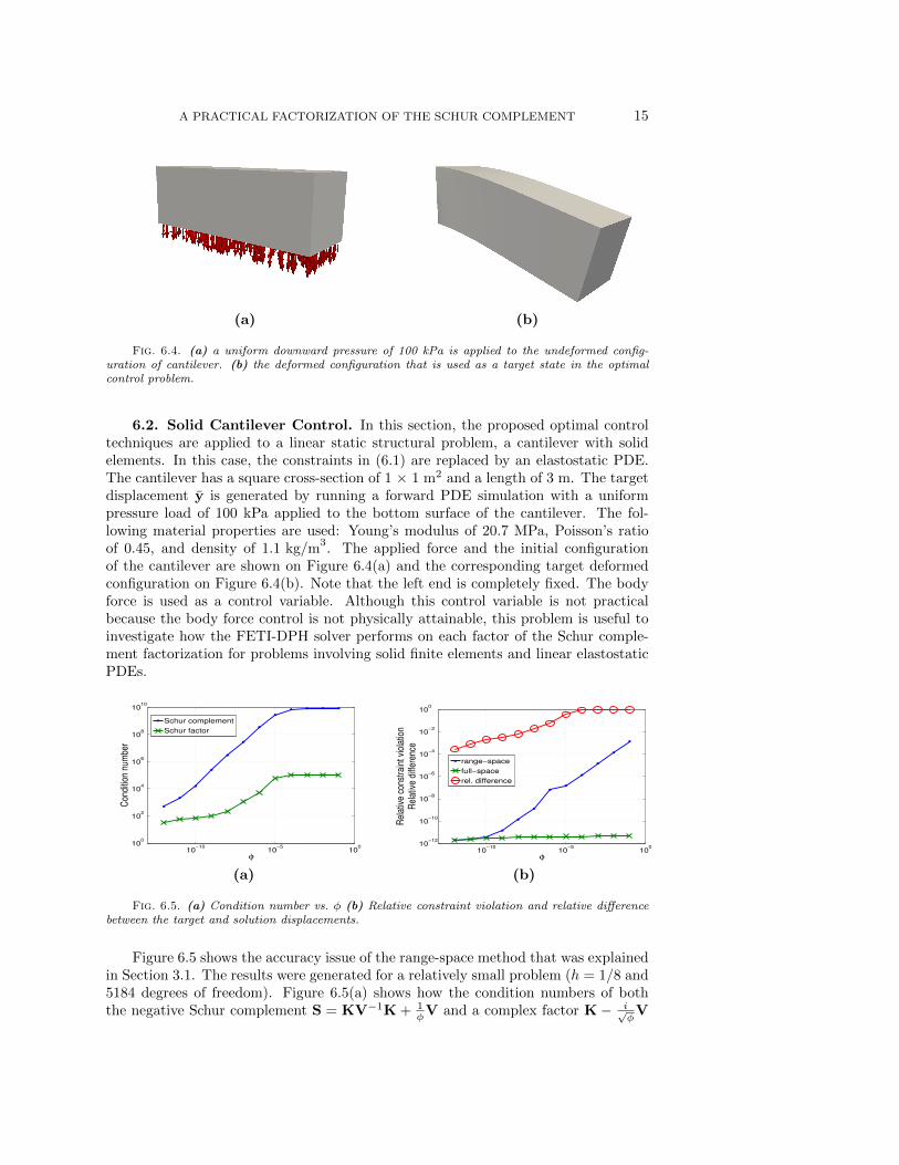
Fig. 6.4. (a) a uniform downward pressure of 100 kPa is applied to the undeformed config-uration of cantilever. (b) the deformed configuration that is used as a target state in the optimalcontrol problem.
6.2. Solid Cantilever Control. In this section, the proposed optimal controltechniques are applied to a linear static structural problem, a cantilever with solidelements. In this case, the constraints in (6.1) are replaced by an elastostatic PDE.The cantilever has a square cross-section of 1 × 1 m2 and a length of 3 m. The targetdisplacement y is generated by running a forward PDE simulation with a uniformpressure load of 100 kPa applied to the bottom surface of the cantilever. The fol-lowing material properties are used: Young’s modulus of 20.7 MPa, Poisson’s ratioof 0.45, and density of 1.1 kg/m
3. The applied force and the initial configuration
of the cantilever are shown on Figure 6.4(a) and the corresponding target deformedconfiguration on Figure 6.4(b). Note that the left end is completely fixed. The bodyforce is used as a control variable. Although this control variable is not practicalbecause the body force control is not physically attainable, this problem is useful toinvestigate how the FETI-DPH solver performs on each factor of the Schur comple-ment factorization for problems involving solid finite elements and linear elastostaticPDEs.
10−10
10−5
100
100
102
104
106
108
1010
φ
Con
ditio
n nu
mbe
r
Schur complement
Schur factor
10−10
10−5
100
10−12
10−10
10−8
10−6
10−4
10−2
100
φ
Rel
ativ
e co
nstr
aint
vio
latio
nR
elat
ive
diffe
renc
e
range−space
full−space
rel. difference
(a) (b)
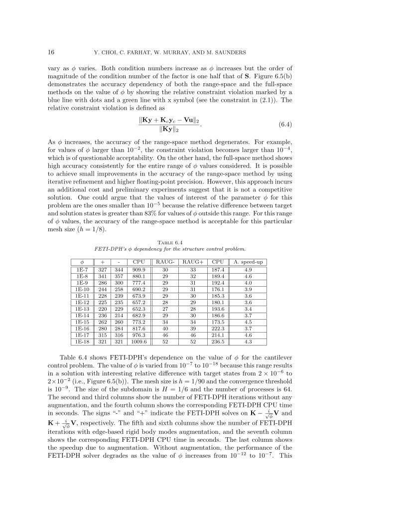
Fig. 6.5. (a) Condition number vs. φ (b) Relative constraint violation and relative differencebetween the target and solution displacements.
Figure 6.5 shows the accuracy issue of the range-space method that was explainedin Section 3.1. The results were generated for a relatively small problem (h = 1/8 and5184 degrees of freedom). Figure 6.5(a) shows how the condition numbers of boththe negative Schur complement S = KV−1K + 1
φV and a complex factor K− i√φV
16 Y. CHOI, C. FARHAT, W. MURRAY, AND M. SAUNDERS
vary as φ varies. Both condition numbers increase as φ increases but the order ofmagnitude of the condition number of the factor is one half that of S. Figure 6.5(b)demonstrates the accuracy dependency of both the range-space and the full-spacemethods on the value of φ by showing the relative constraint violation marked by ablue line with dots and a green line with x symbol (see the constraint in (2.1)). Therelative constraint violation is defined as
‖Ky + Kcyc −Vu‖2‖Ky‖2
. (6.4)
As φ increases, the accuracy of the range-space method degenerates. For example,for values of φ larger than 10−2, the constraint violation becomes larger than 10−4,which is of questionable acceptability. On the other hand, the full-space method showshigh accuracy consistently for the entire range of φ values considered. It is possibleto achieve small improvements in the accuracy of the range-space method by usingiterative refinement and higher floating-point precision. However, this approach incursan additional cost and preliminary experiments suggest that it is not a competitivesolution. One could argue that the values of interest of the parameter φ for thisproblem are the ones smaller than 10−5 because the relative difference between targetand solution states is greater than 83% for values of φ outside this range. For this rangeof φ values, the accuracy of the range-space method is acceptable for this particularmesh size (h = 1/8).
Table 6.4FETI-DPH’s φ dependency for the structure control problem.
φ + - CPU RAUG- RAUG+ CPU A. speed-up
1E-7 327 344 909.9 30 33 187.4 4.91E-8 341 357 880.1 29 32 189.4 4.61E-9 286 300 777.4 29 31 192.4 4.01E-10 244 258 690.2 29 31 176.1 3.91E-11 228 239 673.9 29 30 185.3 3.61E-12 225 235 657.2 28 29 180.1 3.61E-13 220 229 652.3 27 28 193.6 3.41E-14 236 214 682.9 29 30 186.6 3.71E-15 262 260 773.2 34 34 173.5 4.51E-16 280 284 817.6 40 39 222.3 3.71E-17 315 316 976.3 46 46 214.1 4.61E-18 321 321 1009.6 52 52 236.5 4.3
Table 6.4 shows FETI-DPH’s dependence on the value of φ for the cantilevercontrol problem. The value of φ is varied from 10−7 to 10−18 because this range resultsin a solution with interesting relative difference with target states from 2 × 10⁻⁶ to2×10−2 (i.e., Figure 6.5(b)). The mesh size is h = 1/90 and the convergence thresholdis 10−9. The size of the subdomain is H = 1/6 and the number of processes is 64.The second and third columns show the number of FETI-DPH iterations without anyaugmentation, and the fourth column shows the corresponding FETI-DPH CPU timein seconds. The signs “-” and “+” indicate the FETI-DPH solves on K − i√
φV and
K + i√φV, respectively. The fifth and sixth columns show the number of FETI-DPH
iterations with edge-based rigid body modes augmentation, and the seventh columnshows the corresponding FETI-DPH CPU time in seconds. The last column showsthe speedup due to augmentation. Without augmentation, the performance of theFETI-DPH solver degrades as the value of φ increases from 10−12 to 10−7. This
A PRACTICAL FACTORIZATION OF THE SCHUR COMPLEMENT 17
makes sense because the condition number of the complex factors in (4.1) and theSchur complement itself increase as φ increases (see Figure 6.5). However, for therange of smaller φ values (i.e., less than 10−12), the number of FETI-DPH iterationswithout augmentation increases as φ decreases. This is analogous to FETI-DPH beingdependent on wave numbers in acoustic problems if no augmentation is applied (i.e.,more iterations are required for a larger wave number without augmentation) althoughthe complex factors are not the same as in the system that normally arises from aHelmholtz problem. In order to alleviate this deterioration, edge-based rigid bodymode augmentation is used. Table 6.4 shows that the augmentation decreases thenumber of FETI-DPH iterations substantially and reduces the CPU time by a factorof four on average. However, the rigid body modes augmentation is not optimal inthe sense that as φ decreases the number of FETIP-DPH iterations still increases.
Table 6.5 shows the numerical scalability of the FETI-DPH solver for the can-tilever control problem. The number of iterations is shown for various mesh sizesh and for various subdomain sizes H. The regularization parameter φ of 1 × 10⁻¹⁶
is chosen for two reasons. First, the range-space method is not robust for a largevalue of φ. Second, applying the FETI-DPH solver to a small value of φ is morechallenging than applying it to a large value of φ (i.e., Table 6.4). The convergencethreshold for FETI-DPH is 10−9. The problem size is varied from around 2 milliondegrees of freedom to 40 million degrees of freedom. As in the numerical scalabilitytest for the thermal problem, the H/h ratio is fixed to 15 (exactly 3375 elements ineach subdomain) and the number of FETI-DPH iterations is counted for both factorsK − i√
φV and K + i√
φV. As the problem size increases, the number of FETI iter-
ations required for convergence slightly decreases, which is again consistent with thetheoretical result (5.12).
Table 6.5Numerical scalability of the FETI-DPH solver for a fixed φ value for the structure control
problem.
num. of dofs num. of elem. h H nsub K + i√φ
V K− i√φ
V
1,976,400 648,000 1/60 1/4 192 43 433,847,500 1,265,625 1/75 1/5 375 41 406,633,900 2,187,000 1/90 1/6 648 39 38
10,517,850 3,472,875 1/105 1/7 1029 37 3715,681,600 5,184,000 1/120 1/8 1536 36 3622,307,400 7,381,125 1/135 1/9 2187 35 3430,577,500 10,125,000 1/150 1/10 3000 33 3340,674,150 13,476,375 1/165 1/11 3993 33 33
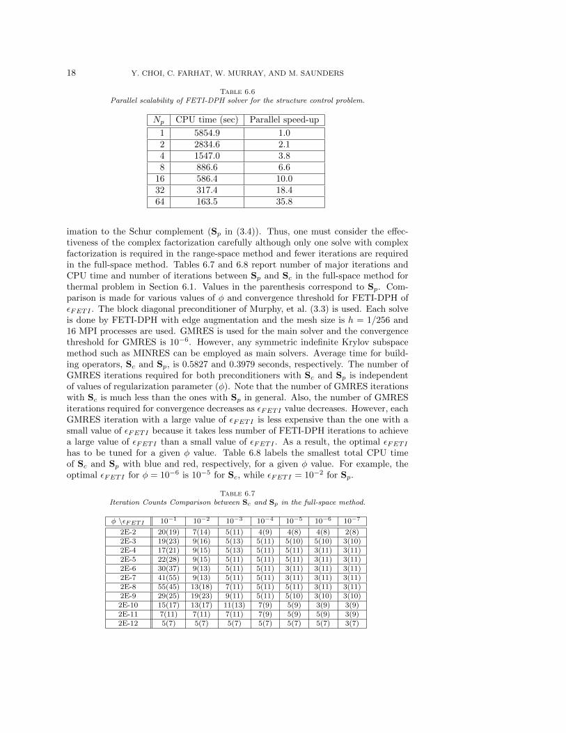
Table 6.6 shows the parallel scalability of FETI-DPH for the cantilever controlproblem. The FETI-DPH CPU time and the corresponding parallel speed-up areshown for the various numbers of processes. The regularization parameter φ is 10−12.The convergence threshold is 10−9. A mesh size h = 1/90 (i.e., around 6.6 milliondegrees of freedom) and a subdomain size H = 1/6 are used. The number of processes(Np) increases from 1 to 64 and parallel speed-up is measured as the ratio with respectto the CPU time of NP = 1. As the number of processes increases up to 64, Table 6.6shows the speed up is greater than half the maximum possible.
6.3. Comparison Between Sc and Sp in the Full-Space Method. Dueto the introduction of complex numbers in the factorization, more storage and morecomputational cost per solve are required compared to Pearson and Wathen’s approx-
18 Y. CHOI, C. FARHAT, W. MURRAY, AND M. SAUNDERS
Table 6.6Parallel scalability of FETI-DPH solver for the structure control problem.
Np CPU time (sec) Parallel speed-up
1 5854.9 1.02 2834.6 2.14 1547.0 3.88 886.6 6.6
16 586.4 10.032 317.4 18.464 163.5 35.8
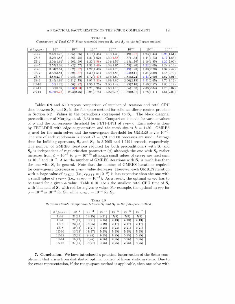
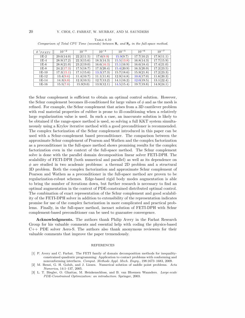
imation to the Schur complement (Sp in (3.4)). Thus, one must consider the effec-tiveness of the complex factorization carefully although only one solve with complexfactorization is required in the range-space method and fewer iterations are requiredin the full-space method. Tables 6.7 and 6.8 report number of major iterations andCPU time and number of iterations between Sp and Sc in the full-space method forthermal problem in Section 6.1. Values in the parenthesis correspond to Sp. Com-parison is made for various values of φ and convergence threshold for FETI-DPH ofεFETI . The block diagonal preconditioner of Murphy, et al. (3.3) is used. Each solveis done by FETI-DPH with edge augmentation and the mesh size is h = 1/256 and16 MPI processes are used. GMRES is used for the main solver and the convergencethreshold for GMRES is 10−6. However, any symmetric indefinite Krylov subspacemethod such as MINRES can be employed as main solvers. Average time for build-ing operators, Sc and Sp, is 0.5827 and 0.3979 seconds, respectively. The number ofGMRES iterations required for both preconditioners with Sc and Sp is independentof values of regularization parameter (φ). Note that the number of GMRES iterationswith Sc is much less than the ones with Sp in general. Also, the number of GMRESiterations required for convergence decreases as εFETI value decreases. However, eachGMRES iteration with a large value of εFETI is less expensive than the one with asmall value of εFETI because it takes less number of FETI-DPH iterations to achievea large value of εFETI than a small value of εFETI . As a result, the optimal εFETIhas to be tuned for a given φ value. Table 6.8 labels the smallest total CPU timeof Sc and Sp with blue and red, respectively, for a given φ value. For example, theoptimal εFETI for φ = 10−6 is 10−5 for Sc, while εFETI = 10−2 for Sp.
Table 6.7Iteration Counts Comparison between Sc and Sp in the full-space method.
φ \εFETI 10−1 10−2 10−3 10−4 10−5 10−6 10−7
2E-2 20(19) 7(14) 5(11) 4(9) 4(8) 4(8) 2(8)2E-3 19(23) 9(16) 5(13) 5(11) 5(10) 5(10) 3(10)2E-4 17(21) 9(15) 5(13) 5(11) 5(11) 3(11) 3(11)2E-5 22(28) 9(15) 5(11) 5(11) 5(11) 3(11) 3(11)2E-6 30(37) 9(13) 5(11) 5(11) 3(11) 3(11) 3(11)2E-7 41(55) 9(13) 5(11) 5(11) 3(11) 3(11) 3(11)2E-8 55(45) 13(18) 7(11) 5(11) 5(11) 3(11) 3(11)2E-9 29(25) 19(23) 9(11) 5(11) 5(10) 3(10) 3(10)2E-10 15(17) 13(17) 11(13) 7(9) 5(9) 3(9) 3(9)2E-11 7(11) 7(11) 7(11) 7(9) 5(9) 5(9) 3(9)2E-12 5(7) 5(7) 5(7) 5(7) 5(7) 5(7) 3(7)
A PRACTICAL FACTORIZATION OF THE SCHUR COMPLEMENT 19
Table 6.8Comparison of Total CPU Time (seconds) between Sc and Sp in the full-space method.
φ \εFETI 10−1 10−2 10−3 10−4 10−5 10−6 10−7
2E-2 2.43(1.78) 1.35(1.66) 1.19(1.45) 1.15(1.38) 1.19(1.37) 1.23(1.44) 0.96(1.51)2E-3 2.26(1.83) 1.56(1.78) 1.21(1.62) 1.30(1.58) 1.37(1.62) 1.44(1.73) 1.17(1.83)2E-4 2.01(1.64) 1.56(1.59) 1.22(1.58) 1.34(1.59) 1.43(1.76) 1.16(1.85) 1.20(2.00)2E-5 2.57(2.09) 1.82(1.57) 1.31(1.46) 1.39(1.65) 1.53(1.80) 1.22(2.00) 1.28(2.16)2E-6 3.04(2.54) 1.62(1.37) 1.27(1.49) 1.47(1.76) 1.19(1.98) 1.30(2.20) 1.37(2.42)2E-7 3.65(3.81) 1.59(1.37) 1.30(1.54) 1.56(1.83) 1.24(2.11) 1.34(2.39) 1.48(2.70)2E-8 4.88(2.77) 1.95(1.59) 1.72(1.47) 1.57(1.80) 1.85(2.22) 1.43(2.60) 1.62(3.01)2E-9 2.49(1.64) 2.31(1.75) 1.91(1.33) 1.63(1.80) 2.00(2.15) 1.51(2.65) 1.70(3.12)2E-10 1.55(1.23) 1.56(1.22) 1.95(1.25) 2.06(1.49) 1.99(2.10) 1.56(2.57) 1.83(3.12)2E-11 1.05(0.97) 1.03(0.93) 1.21(0.96) 1.63(1.16) 1.65(1.68) 2.38(2.34) 1.78(3.07)2E-12 0.91(0.73) 0.93(0.76) 0.94(0.75) 1.02(0.78) 1.32(0.97) 1.78(1.41) 1.61(2.00)
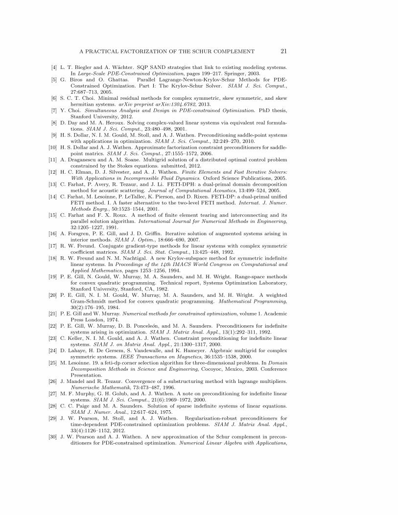
Tables 6.9 and 6.10 report comparison of number of iteration and total CPUtime between Sp and Sc in the full-space method for solid cantilever control problemin Section 6.2. Values in the parenthesis correspond to Sp. The block diagonalpreconditioner of Murphy, et al. (3.3) is used. Comparison is made for various valuesof φ and the convergence threshold for FETI-DPH of εFETI . Each solve is doneby FETI-DPH with edge augmentation and the mesh size is h = 1/30. GMRESis used for the main solver and the convergence threshold for GMRES is 2 × 10⁻⁶.The size of each subdomain is about H = 1/3 and 60 processes are used. Averagetime for building operators, Sc and Sp, is 3.7695 and 1.2191 seconds, respectively.The number of GMRES iterations required for both preconditioners with Sc andSp is independent of regularization parameter (φ) although the one with Sp ratherincreases from φ = 10−2 to φ = 10−10 although small values of εFETI are used suchas 10−6 and 10−7. Also, the number of GMRES iterations with Sc is much less thanthe one with Sp in general. Note that the number of GMRES iterations requiredfor convergence decreases as εFETI value decreases. However, each GMRES iterationwith a large value of εFETI (i.e., εFETI = 10−2) is less expensive than the one witha small value of εFETI (i.e., εFETI = 10−7). As a result, the optimal εFETI has tobe tuned for a given φ value. Table 6.10 labels the smallest total CPU time of Scwith blue and of Sp with red for a given φ value. For example, the optimal εFETI forφ = 10−6 is 10−5 for Sc, while εFETI = 10−4 for Sp.
Table 6.9Iteration Counts Comparison between Sc and Sp in the full-space method.
φ \εFETI 10−2 10−3 10−4 10−5 10−6 10−7
1E-2 21(21) 13(15) 9(11) 7(9) 7(9) 7(9)1E-4 21(27) 13(21) 9(15) 7(13) 7(13) 7(13)1E-6 23(33) 15(25) 9(19) 7(17) 7(17) 7(17)1E-8 19(33) 11(27) 9(25) 7(23) 7(21) 7(21)1E-10 13(33) 11(27) 7(25) 7(25) 7(25) 7(25)1E-12 13(29) 9(25) 7(25) 7(25) 5(25) 5(25)1E-14 15(27) 9(25) 7(25) 7(25) 5(25) 5(25)1E-16 27(37) 15(27) 9(25) 7(25) 7(25) 5(25)
7. Conclusion. We have introduced a practical factorization of the Schur com-plement that arises from distributed optimal control of linear static systems. Due tothe exact representation, if the range-space method is applicable, then one solve with
20 Y. CHOI, C. FARHAT, W. MURRAY, AND M. SAUNDERS
Table 6.10Comparison of Total CPU Time (seconds) between Sc and Sp in the full-space method.
φ \εFETI 10−2 10−3 10−4 10−5 10−6 10−7
1E-2 29.0(14.0) 22.2(11.5) 17.6(9.9) 15.9(9.7) 17.7(10.2) 17.9(11.1)1E-4 28.9(17.2) 22.3(15.6) 18.3(14.3) 15.5(13.8) 16.8(14.3) 17.7(15.9)1E-6 28.8(21.0) 23.2(19.0) 16.6(16.3) 15.1(16.9) 16.6(18.4) 17.4(21.0)1E-8 24.2(17.3) 17.5(18.7) 17.3(20.4) 15.4(20.9) 16.3(20.9) 17.2(23.5)1E-10 17.3(15.1) 17.1(15.6) 13.3(17.3) 15.7(18.6) 15.9(21.8) 17.2(23.3)1E-12 13.4(9.6) 11.4(10.7) 11.1(11.8) 12.9(14.8) 10.8(17.0) 11.6(20.3)1E-14 14.3(8.8) 12.3(10.5) 12.7(13.2) 14.1(16.2) 12.0(19.5) 13.1(22.4)1E-16 15.5(7.8) 15.9(9.0) 13.9(12.1) 14.5(15.4) 19.7(19.8) 14.9(24.1)
the Schur complement is sufficient to obtain an optimal control solution. However,the Schur complement becomes ill-conditioned for large values of φ and as the mesh isrefined. For example, the Schur complement that arises from a 3D cantilever problemwith real material properties of rubber is prone to ill-conditioning when a relativelylarge regularization value is used. In such a case, an inaccurate solution is likely tobe obtained if the range-space method is used, so solving a full KKT system simulta-neously using a Krylov iterative method with a good preconditioner is recommended.The complex factorization of the Schur complement introduced in this paper can beused with a Schur-complement based preconditioner. The comparison between theapproximate Schur complement of Pearson and Wathen and the complex factorizationas a preconditioner in the full-space method shows promising results for the complexfactorization even in the context of the full-space method. The Schur complementsolve is done with the parallel domain decomposition linear solver FETI-DPH. Thescalability of FETI-DPH (both numerical and parallel) as well as its dependence onφ are studied in two academic problems: a thermal 2D problem and a structural3D problem. Both the complex factorization and approximate Schur complement ofPearson and Wathen as a preconditioner in the full-space method are proven to beregularization-robust schemes. Edge-based rigid body modes augmentation is ableto bring the number of iterations down, but further research is necessary to find anoptimal augmentation in the context of PDE-constrained distributed optimal control.The combination of exact representation of the Schur complement and good scalabil-ity of the FETI-DPH solver in addition to extensibility of the representation indicatespromise for use of the complex factorization in more complicated and practical prob-lems. Finally, in the full-space method, inexact solution of FETI-DPH with Schurcomplement-based preconditioner can be used to guarantee convergence.
Acknowledgments. The authors thank Philip Avery in the Farhat ResearchGroup for his valuable comments and essential help with coding the physics-basedC++ PDE solver Aero-S. The authors also thank anonymous reviewers for theirvaluable comments that improve the paper tremendously.
REFERENCES
[1] P. Avery and C. Farhat. The FETI family of domain decomposition methods for inequality-constrained quadratic programming: Application to contact problems with conforming andnonconforming interfaces. Comput. Methods Appl. Mech. Engrg., 198:1673–1683, 2009.
[2] M. Benzi, G. H. Golub, and J. Liesen. Numerical solution of saddle point problems. ActaNumerica, 14:1–137, 2005.
[3] L. T. Biegler, O. Ghattas, M. Heinkenschloss, and B. van Bloemen Waanders. Large-scalePDE-Constrained Optimization: an introduction. Springer, 2003.
A PRACTICAL FACTORIZATION OF THE SCHUR COMPLEMENT 21
[4] L. T. Biegler and A. Wachter. SQP SAND strategies that link to existing modeling systems.In Large-Scale PDE-Constrained Optimization, pages 199–217. Springer, 2003.
[5] G. Biros and O. Ghattas. Parallel Lagrange-Newton-Krylov-Schur Methods for PDE-Constrained Optimization. Part I: The Krylov-Schur Solver. SIAM J. Sci. Comput.,27:687–713, 2005.
[6] S. C. T. Choi. Minimal residual methods for complex symmetric, skew symmetric, and skewhermitian systems. arXiv preprint arXiv:1304.6782, 2013.
[7] Y. Choi. Simultaneous Analysis and Design in PDE-constrained Optimization. PhD thesis,Stanford University, 2012.
[8] D. Day and M. A. Heroux. Solving complex-valued linear systems via equivalent real formula-tions. SIAM J. Sci. Comput., 23:480–498, 2001.
[9] H. S. Dollar, N. I. M. Gould, M. Stoll, and A. J. Wathen. Preconditioning saddle-point systemswith applications in optimization. SIAM J. Sci. Comput., 32:249–270, 2010.
[10] H. S. Dollar and A. J. Wathen. Approximate factorization constraint preconditioners for saddle-point matrics. SIAM J. Sci. Comput., 27:1555–1572, 2006.
[11] A. Draganescu and A. M. Soane. Multigrid solution of a distributed optimal control problemconstrained by the Stokes equations. submitted, 2012.
[12] H. C. Elman, D. J. Silvester, and A. J. Wathen. Finite Elements and Fast Iterative Solvers:With Applications in Incompressible Fluid Dynamics. Oxford Science Publications, 2005.
[13] C. Farhat, P. Avery, R. Tezaur, and J. Li. FETI-DPH: a dual-primal domain decompositionmethod for acoustic scattering. Journal of Computational Acoustics, 13:499–524, 2005.
[14] C. Farhat, M. Lesoinne, P. LeTallec, K. Pierson, and D. Rixen. FETI-DP: a dual-primal unifiedFETI method. I. A faster alternative to the two-level FETI method. Internat. J. Numer.Methods Engrg., 50:1523–1544, 2001.
[15] C. Farhat and F. X. Roux. A method of finite element tearing and interconnecting and itsparallel solution algorithm. International Journal for Numerical Methods in Engineering,32:1205–1227, 1991.
[16] A. Forsgren, P. E. Gill, and J. D. Griffin. Iterative solution of augmented systems arising ininterior methods. SIAM J. Optim., 18:666–690, 2007.
[17] R. W. Freund. Conjugate gradient-type methods for linear systems with complex symmetriccoefficient matrices. SIAM J. Sci. Stat. Comput., 13:425–448, 1992.
[18] R. W. Freund and N. M. Nachtigal. A new Krylov-subspace method for symmetric indefinitelinear systems. In Proceedings of the 14th IMACS World Congress on Computational andApplied Mathematics, pages 1253–1256, 1994.
[19] P. E. Gill, N. Gould, W. Murray, M. A. Saunders, and M. H. Wright. Range-space methodsfor convex quadratic programming. Technical report, Systems Optimization Laboratory,Stanford University, Stanford, CA, 1982.
[20] P. E. Gill, N. I. M. Gould, W. Murray, M. A. Saunders, and M. H. Wright. A weightedGram-Schmidt method for convex quadratic programming. Mathematical Programming,30(2):176–195, 1984.
[21] P. E. Gill and W. Murray. Numerical methods for constrained optimization, volume 1. AcademicPress London, 1974.
[22] P. E. Gill, W. Murray, D. B. Ponceleon, and M. A. Saunders. Preconditioners for indefinitesystems arising in optimization. SIAM J. Matrix Anal. Appl., 13(1):292–311, 1992.
[23] C. Keller, N. I. M. Gould, and A. J. Wathen. Constraint preconditioning for indefinite linearsystems. SIAM J. on Matrix Anal. Appl., 21:1300–1317, 2000.
[24] D. Lahaye, H. De Gersem, S. Vandewalle, and K. Hameyer. Algebraic multigrid for complexsymmetric systems. IEEE Transactions on Magnetics, 36:1535–1538, 2000.
[25] M. Lesoinne. 19. a feti-dp corner selection algorithm for three-dimensional problems. In DomainDecomposition Methods in Science and Engineering, Cocoyoc, Mexico, 2003. ConferencePresentation.
[26] J. Mandel and R. Tezaur. Convergence of a substructuring method with lagrange multipliers.Numerische Mathematik, 73:473–487, 1996.
[27] M. F. Murphy, G. H. Golub, and A. J. Wathen. A note on preconditioning for indefinite linearsystems. SIAM J. Sci. Comput., 21(6):1969–1972, 2000.
[28] C. C. Paige and M. A. Saunders. Solution of sparse indefinite systems of linear equations.SIAM J. Numer. Anal., 12:617–624, 1975.
[29] J. W. Pearson, M. Stoll, and A. J. Wathen. Regularization-robust preconditioners fortime-dependent PDE-constrained optimization problems. SIAM J. Matrix Anal. Appl.,33(4):1126–1152, 2012.
[30] J. W. Pearson and A. J. Wathen. A new approximation of the Schur complement in precon-ditioners for PDE-constrained optimization. Numerical Linear Algebra with Applications,
22 Y. CHOI, C. FARHAT, W. MURRAY, AND M. SAUNDERS
19:816–829, 2012.[31] E. Prudencio, R. Byrd, and X. C. Cai. Parallel full space SQP Lagrange-Newton-Krylov-
Schwarz algorithms for PDE-constrained optimization problems. SIAM J. Sci. Comput.,27:13051328, 2006.
[32] T. Rees, H. S. Dollar, and A. J. Wathen. Optimal solvers for PDE-constrained optimization.SIAM J. Sci. Comput., 32:271–298, 2010.
[33] S. Reitzinger, U. Schreiber, and U. Van Rienen. Algebraic multigrid for complex symmetricmatrices and applications. Journal of computational and applied mathematics, 155(2):405–421, 2003.
[34] Y. Saad and M. H. Schultz. GMRES: A generalized minimal residual algorithm for solvingnonsymmetric linear systems. SIAM J. Sci. Stat. Comput., 7, 1986.
[35] V. Simoncini. Reduced order solution of structured linear systems arising in certainPDE-constrained optimization problems. Computational Optimization and Applications,53(2):591–617, 2012.
[36] M. Stoll and A. Wathen. Combination preconditioning and the Bramble-Pasciak+ precondi-tioner. SIAM Journal on Matrix Anal. Appl., 2011.
[37] H. S. Thorne. Properties of linear systems in PDE-constrained optimization. Part I: Distributedcontrol. Technical report, Rutherford Appleton Laboratory, 2009.
[38] H. S. Thorne. Properties of linear systems in PDE-constrained optimization. Part II: Neumannboundary control. Technical report, Rutherford Appleton Laboratory, 2009.